


1. INTRODUCTION
Theoretical and experimental study of evolution of high power laser beam, as they propagate through plasmas, is an active area of research due to their potential relevance as plasma based accelerators (Sarkisov et al., Reference Sarkisov, Bychenkov, Novikov, Tikhonchuk, Maksimchuk, Chen, Wagner, Mourou and Umstadter1999), inertial confinement fusion (Tabak et al., Reference Tabak, Hammer, Glinsky, Kruer, Wilks, Woodworth, Campbell, Perry and Mason1994; Regan et al., Reference Regan, Bradley, Chirokikh, Craxton, Meyerhofer, Seka, Short, Simon, Town and Yaakobi1999), and new radiation sources (Suckewer & Skinner, Reference Suckewer and Skinner1990, Reference Suckewer and Skinner1995; Benware et al., Reference Benware, Macchietto, Moreno and Rocca1998; Yu et al., Reference Yu, Yu, Zhang and Xu1998; Foldes et al., Reference Foldes, Bakos, Bakonyi, Nagy and Szatmari1999; Fedotov et al., Reference Fedotov, Naumov, Silin, Uryupin, Zheltikov, Tarasevitch and Von der Linde2000). For success of these applications, a long distance propagation of intense lasers in plasma is desirable. For example, in laser fusion, the coupling and the propagation of the laser beams in the plasma surrounding the pellet must be well controlled to produce high energy level. As laser beam propagates through plasma, many instabilities and nonlinear phenomena such as self-phase modulation, the filamentation instability, group velocity dispersion, finite pulse effects, relativistic and ponderomotive self-focusing effects, become important. This implies a deep understanding of laser plasma interaction physics to keep the nonlinear process at low level.
The self-focusing, a genuinely nonlinear basic phenomenon, which plays crucial role in beam propagation, arises due to increase of the on-axis index of refraction relative to edge of the laser beam. For example, for ponderomotive force type nonlinearity, we have expulsion of electrons from the region of high intensity laser field. Relativistic self-focusing results from the effect of quiver motion leading to reduced local plasma frequency. The self-focusing is counter-balanced by the tendency of the beam to spread because of diffraction. In the absence of nonlinearities, the beam will spread substantially in a Rayleigh length, R d ~ k 0r 02. Self-focusing and filamentation are among the most dangerous nonlinear phenomena, which destroy the uniformity of overall irradiation required for direct-drive fusion experiment as well as leads to seeding and growth of hydrodynamic instabilities. Experimental as well as theoretical observations of relativistic self-focusing and ponderomotive self-channeling have been reported in a number of investigations (Borisov et al., Reference Borisov, Borovskiy, Korobkin, Prokhorov, Shiryaev, Shi, Luk, McPherson, Solem, Boyer and Rhodes1992, Reference Borisov, Longworth, Boyer and Rhodes1998; Faenov et al., Reference Faenov, Magunov, Pikuz, Skobelev, Gasilov, Stagira, Calegari, Nisoli, De Silvestri, Poletto, Villoresi and Andreev2007; Chessa et al., Reference Chessa, Mora and Antonsen1998; Sun et al., Reference Sun, Ott, Lee and Guzdar1987; Kurki-Suonio et al., Reference Kurki-Suonio, Morrison and Tajima1989; Abramyan et al., Reference Abramyan, Litvak, Mironov and Sergeev1992; Chen & Sudan, Reference Chen and Sudan1993; Tzeng & Mori, Reference Tzeng and Mori1998; Monot et al., Reference Monot, Auguste, Gibbon, Jakober, Mainfray, Dulieu, Louis-Jacquet, Malka and Miquel1995; Krushelnick et al., Reference Krushelnick, Ting, Moore, Burris, Esarey, Sprangle and Baine1997; Konar & Manoj, Reference Konar and Manoj2005; Wagner et al., Reference Wagner, Chen, Maksimuchuk and Umstadter1997; Chen et al., Reference Chen, Sarkisov, Maksimchuk, Wagner and Umstadter1998). The dynamics of ponderomotive channeling in underdense plasma has recently been studied experimentally (Borghesi et al., Reference Borghesi, Kar, Romagnani, Toncian, Antici, Audebert, Brambrink, Ceccherini, Cecchetti, Fuchs, Galimberti, Gizzi, Grismayer, Lyseikina, Jung, Macchi, Mora, Osterholtz, Schiavi and Willi2007). Relativistic laser-plasma interaction physics has also been a focus of attention as many nonlinear processes playing key roles in the generation of new ion sources has been reported recently (Laska et al., Reference Laska, Badziak, Boody, Gammino, Jungwirth, Krasa, Krousky, Parys, Pfeifer, Rohlena, Ryc, Skala, Torrisi, Ullschmied and Wolowski2007; Torrisi et al., Reference Torrisi, Margarone, Laska, Krasa, Velyhan, Pfeifer, Ullschmied and Ryc2008; Strangio et al., Reference Strangio, Caruso, Neely, Andreoli, Anzalone, Clarke, Cristofari, DelPrete, Di Giorgio, Murphy, Ricci, Stevens and Tolley2007). Since ponderomotive and relativistic channeling occur together, we investigate their combined effects on the evolution of intense laser beam in non-uniform plasma channel. Plasma channels are important as they act as a duct to guide laser beams over long distance of propagation. Further, the novel experiments to study rich physics issues in nuclear and particle physics, atomic physics (Stoehlker et al., Reference Stoehlker, Backe, Beyer, Bosch, Braeuning-Demian, Hagman, Ionescu, Jungmann, Kluge, Kozhuharov, Kuehl, Lisen, Mann, Mokler and Quint2003), plasma physics (Hoffmann et al., Reference Hoffmann, Blazevic, Ni, Rosmej, Roth, Tahir, Tauschwitz, Udrea, Varentsov, Weyrich and Maron2005; Schaumann et al., Reference Schaumann, Schollmeier, Rodriguez-Prieto, Blazevic, Brambrink, Geissel, Korostiy, Pirzadeh, Roth, Rosmej, Faenov, Pikuz, Tsigutkin, Maron, Tahir and Hoffmann2005), and applied sciences (Kuehl et al., Reference Kuehl, Ursescu, Bagnoud, Javorkova, Rosmej, Cassou, Kazamias, Klisnick, Ros, Nickles, Zielbauer, Dunn, Neumayer and Pert2007; Kasperczuk et al., Reference Kasperczuk, Pisarczyk, Kalal, Martinkova, Ullschmied, Krousky, Masek, Pfeifer, Rohlena, Skala and Pisarczyk2008) has opened new vistas in this field and has given a multidisciplinary character to laser produced plasmas. Most general form of the field envelope in the absence of dispersion and under slowly varying envelope approximation is:

Eq. (1) also known as the nonlinear Schrödinger equation, is a nonlinear parabolic partial differential equation type governing field envelope of laser electromagnetic beam during its propagation in a nonlinear medium. Thus, conventional separable techniques using Fourier expansions are not applicable. These higher dimensional nonlinear Schrödinger equations (NLSE) are not integrable so that they do not have special solution such as soliton solutions. However, they possess stationary solution, which are unstable on propagation. For deeper insight into the physical process, we solve Eq. (1) by using some analytical approximate models. Thus, the resulting solutions provide qualitative rather than quantitative estimates.
Some of the approximate theories used to study self-focusing process are a paraxial ray approximation (Akhmanov et al., Reference Akhmanov, Sukhorukov and Khokhlov1968; Sodha et al., Reference Sodha, Ghatak and Tripathi1974, Reference Sodha, Ghatak and Tripathi1976), moment theory approach (Firth, Reference Firth1977; Lam et al., Reference Lam, Lippmann and Tappert1975, Reference Lam, Lippmann and Tappert1977), variational approach (Firth, Reference Firth1977; Anderson & Bonnedal, Reference Anderson and Bonnedal1979), and source-dependent expansion (SDE) method (Sprangle et al., Reference Sprangle, Hafizi and Penano2000). Each of these theories has limitations in describing completely the experimental/computer simulation results. However, the mostly used theory based on Wentzel-Krammers-Brillouin approximation and paraxial ray approach is given by Akhmanov et al. (Reference Akhmanov, Sukhorukov and Khokhlov1968) and developed by Sodha et al. (Reference Sodha, Ghatak and Tripathi1976). Due to its mathematical simplicity, it has been extensively used to account for general features of self-focusing as witnessed by the increasing number of publications. However, this theory being local in character over-emphasizes the field closest to beam axis and lacks global pulse dynamics. Furthermore, it also predicts unphysical phase relationship (Karlsson et al., Reference Karlsson, Anderson, Desaix and Lisak1991). It has been pointed out that paraxial ray theory is not applicable when high power laser beams are used (Subbarao et al., Reference Subbarao, Uma and Singh1998). With some partial remedies to paraxial ray theory, the moment theory of self-focusing gives results closer to computer simulations. However, this theory was not actively pursued as it lacks generalization and phase description. Another global approach is variational approach, although crude to describe the singularity formation and collapse dynamics is general in nature to describe the propagation and correctly predicts the phase.
In most of the earlier investigations on self-focusing, carrier distributions takes place on the transverse wave front of the laser beam, leading to inhomogeneity in the plane transverse to beam propagation direction, where refractive index profile is modified on wave front transverse to beam propagation direction. In real physical situation, the laser beam propagates in the underdense plasma up to critical surface, which is spatially inhomogeneous, both in longitudinal and transverse directions. In this underdense plasma, several parametric processes occur before the critical surface is approached. Several nonlinear processes occur due to self-focusing as reported in a number of recent experiments (Torrisi et al., Reference Torrisi, Margarone, Laska, Krasa, Velyhan, Pfeifer, Ullschmied and Ryc2008; Faenov et al., Reference Faenov, Magunov, Pikuz, Skobelev, Gasilov, Stagira, Calegari, Nisoli, De Silvestri, Poletto, Villoresi and Andreev2007). Moreover, (2 + 1)-dimensional self-focusing that is guided in both transverse directions is unstable under collapse (Berge, Reference Berge1998). In an earlier investigation, two dimensional self-focusing of laser beam in an inhomogeneous laser produced plasma is studied (Gill et al., Reference Gill, Saini and Kaul2001). The effect of inhomogeneity of scale lengths is introduced (Andreev et al., Reference Andreev, Erokhin, Sutyagin and Fadeev1987). Since diffraction and nonlinearities in-play takes at different spatial characteristic lengths, we have introduced d(z) and λ(z) as two scale lengths for varying diffraction and nonlinearity. We have introduced this feature phenomenologically to simulate the realistic situations. With the advancement of laser science and pulse shaping technology along with the novel idea of light controlling light, it may be possible to tailor underdense plasma in which diffraction, dispersion and nonlinearity can be controlled. The problem is akin to dispersion and nonlinearity management of laser beam propagation in nonlinear fiber optics (Ablowitz & Mussliamani, Reference Ablowitz and Mussliamani2003; Matuszewski et al., Reference Matuszewski, Trippenbach, Malomed, Infeld and Skorupski2004; Abdullaev et al., Reference Abdullaev, Baizakov and Salerno2003). Further, we can control these parameters to prevent the collapse of the beam due to strong self-focusing.
The organization of the paper is as follows: In Section 2, a model is set up in a weakly relativistic limit starting from Maxwell's equations and hydrodynamic equations. These equations under approximate conditions lead to an evolution equation. Lagrangian for the problem is set up and variational approach is used. Section 3 is devoted to discussion, and in Section 4, we study the stability characteristics of the laser beam. In the last, Section 5, conclusions of present investigation are presented.
2. BASIC FORMULATION
The present model is set up in a weakly relativistic limit starting from Maxwell's equations and hydrodynamic equations. Two coupled equations for density perturbation and laser beam vector potential in a preformed plasma channel (Hafizi et al., Reference Hafizi, Ting, Sprangle and Hubbard2000, Reference Hafizi, Ting, Hubbard, Sprangle and Penano2003; Panwar & Sharma, Reference Panwar and Sharma2009; Duda & Mori, Reference Duda and Mori2000) are given as follows:


where ψ is the vector potential normalized by  , m 0 and e are the rest mass and charge of electron, c is the velocity of light in vacuum. n 0 is the initial axial electron density, and δn is the perturbed electron density, respectively. r ch is the effective channel radius.
The effect of inhomogeneity with two scale lengths was first introduced by Andreev et al. (Reference Andreev, Erokhin, Sutyagin and Fadeev1987) and later used by Gill et al. (Reference Gill, Saini and Kaul2001) using variational approach has been introduced. We have assumed parabolic density profile and long pulse limit approximation (Liu et al., Reference Liu, Guo, Zhou, Li, Li and Wu2004) along with slowly varying envelope approximation. On introducing characteristic scale length d(z) of diffraction and λ(z) for nonlinearity, we obtain the following evolution equation governing the electric field envelope in collisionless plasmas as follows:

We further assume d(z) = d 0 + d 1(z), λ(z) = λ0 + λ1(z).
Eq. (4) is a special case of Eq. (1) and is a nonlinear parabolic partial differential equation in which the second term has its origin in diffractional divergence along with diffraction management coefficient, the term within parenthesis corresponds to channel, ponderomotive self-focusing (PSF), and relativistic self-focusing (RSF), respectively. Variational approach that have rigorous basis, as applied in other fields, is used here to investigate nonlinear wave propagation. It may also be mentioned that we have assumed parabolic profile for the plasma channel. We use the procedure of Anderson and Bonnedal (Reference Anderson and Bonnedal1979) to reformulate Eq. (4) into a variational problem corresponding to a Lagrangian L, so as to make  . Thus, Lagrangian L corresponding to Eq. (4) is given by:
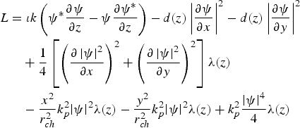
Thus, the solution to the variational problem

which also solves the nonlinear Schrödinger Eq. (4). Using the trial function as Gaussian beam of the form as:

where a(z) is the beam width, b(z) is the spatial chirp, and ϕ(z) is the phase of the laser beam. Using the ansatz, with expression for ψ as the trial function, we can perform the integration to write:

Using the procedure of Anderson and Bonnedal (Reference Anderson and Bonnedal1979) and Saini and Gill, Reference Saini and Gill2006), we arrive at the following equations for a, ϕ:

The second term in Eq. (9) is neglected assuming  as slowly varying with respect to other terms.

After normalization, using η = kz, we get the following equations:


Euler-Lagrange equations can also be algebraically manipulated to yield

where N is the conserved quantity associated with the energy of the beam. The energy of the beam is given by:

Rearranging Eq. (9), we get:

where

Thus, Hamiltonian  of the system is given as follows:

When coefficient of diffraction and nonlinearity are constants, total energy is conserved and is given by:

where

We phenomenologically introduce diffraction and nonlinearity as periodically varying functions in the form d(z) = d 0 + d 1SinΩ(z), λ(z) = λ0 + λ1SinΩ(z). Such variations are generally considered for soliton propagation in optical fiber for long propagation through diffraction and nonlinearity management. Advancement in laser technology can cater to pulse shaping of laser beams/pulses, which may be proposed for similar profiles of d(z) and λ(z). However, in laser plasma interaction, we here introduce such paradigm phenomenologically. Eq. (9) can be treated analytically by means of Kapitsa averaging method (Landau & Lifshitz, Reference Landau and Lifshitz1976). Substituting a(z) = a′0(z) + ρ(z) in Eq. (9) and separating the resulting equation into rapidly varying and slowly varying parts as:


where over-line indicates the average value. Integrating Eq. (20) twice, we obtain:

Substituting Eq. (22) into Eq. (21), we obtain the equation of motion for the slowly varying part as:

where

Hence, the effective potential U for the system is given by:

3. DISCUSSION
Eq. (11) describes the beam dynamics in plasma with relativistic, ponderomotive self-channeling along with channel focusing. The Eqs. (11) and (12) are nonlinearly coupled ordinary second order differential equations governing the beam width parameter a and phase ϕ. There are several terms appearing on right-hand-side (r.h.s.) of both Eqs. (11) and (12). Further, Eq. (12) describes the longitudinal phase. Analytical solutions to these equations are not possible. We therefore seek numerical computational techniques to study beam dynamics. Before that, it is worth noting to understand the physical mechanisms and origin of various terms on the r.h.s. of Eq. (11). The first term on the r.h.s. of Eq. (11) is responsible for diffractional divergence of the laser beam. It has its origin in the Laplacian (∇⊥2) appearing in the evolution Eq. (4). The other terms represent the combined effects of RSF, PSF, and self-channeling (SC). Self-focusing/defocusing of laser beam in plasma is determined by the competing mechanisms on the r.h.s. of Eq. (11). The normalized beam width parameter, a < 1 corresponds to self-focusing and a > 1 is the result of diffractional dominance over all other terms leading to defocusing of laser beam. In the absence of these terms, beam diverges due to diffraction. However, as mentioned in the Introduction, long distances of several Rayleigh lengths are prerequisite for novel applications of laser-produced plasma. In contrast to earlier research work, where relativistic and ponderomotive self-focusing using different approaches have been reported, the present investigation makes use of variational approach along with diffraction and nonlinearity management. We have considered all three mechanisms in our analysis to understand the combined role of RSF, PSF, and SC. To study the propagation characteristics, it is important to observe the evolution of beam width and self-phase modulation with distance of propagation. In order to observe the role of nonlinearity and diffraction management, we have chosen the following set of parameters for numerical computation of normalized beam width as a function of distance of propagation, η.

The results are displayed in the form of graphs for three different values of intensity parameter, |ψ0|2. In this case, apparently control parameter,  is unity. It is observed from Figure 1 that oscillatory self-focusing takes place in all three cases of intensity. However, there is substantial increase in self-focusing with increase in |ψ0|2. It is further important to notice that beam propagates oscillatory and infinitely over several number of Rayleigh lengths (Fauser & Langhoff, Reference Fauser and Langhoff2000). On the other hand, longitudinal phase is both positive as well as negative depending on the mechanism incorporated in the beam dynamics as shown in Figure 2. However, regularized phase is always negative [not shown]. Last, we analyze the effect of management control parameter R dλ. We choose the following set of parameters:

(Color online) Variation of normalized beam width a(z) with normalized distance of propagation η for constant diffraction and nonlinearity with the following set of parameters: Solid curve corresponds to intensity parameter |ψ0|2 = 0.8. Dotted curve corresponds to |ψ0|2 = 0.99. Dashed curve corresponds to |ψ0|2 = 1.2.

(Color online) Plot of longitudinal phase ϕ versus normalized distance of propagation η for the same parameters as mentioned in the caption of Figure 1. Solid curve corresponds to intensity parameter |ψ0|2 = 0.8. Dotted curve corresponds to |ψ0|2 = 0.99. Dashed curve corresponds to |ψ0|2 = 1.2.

The results of numerical computation are shown in the form of graphs. As obvious from Figure 3, there is a substantial decrease in the value of |ψ0|2 for oscillatory self-focusing, which highlights the role of diffraction and nonlinearity management. The plot of longitudinal phase is shown in Figure 4. For comparative study of RSF, PSF, and CF, we first consider the case of various equilibrium radiuses when the channel term is absent. In this case, as usual, the propagation of laser beam in self-trapped mode is analyzed by putting  in Eq. (9) and a = a 0, the initial value of beam width. The results displayed in the form of graphs are plotted in Figure 5 for the three values of R dλ. The solid curve represents the case when diffraction and nonlinearity parameters are equal. We observe monotonic fall of equilibrium radius with increase in |ψ0|2. However, when R dλ is decreased, initially faster fall in
 with |ψ0|2 becomes much slower with further increase in |ψ0|2. Finally, radius becomes almost independent of |ψ0|2. Similar results are investigated in the presence of three mechanisms viz RSF + PSF + CF ≠ 0 as shown in Figure 6. We study again the normalized equilibrium radius as a function of |ψ0|2 for three values of R dλ. The following important observations are made: (1) Normalized equilibrium radius is much smaller than case 1. (2) Decrease in value of R dλ leads to initially faster fall in
 , variation of which becomes slower with increase in |ψ0|2. (3) Stabilization of
 with |ψ0|2 is obtained for higher values of |ψ0|2.
(Color online) Variation of normalized beam width a(z) with normalized distance of propagation η for periodically varying diffraction and nonlinearity with the same set of parameters as in the caption of Figure 1 with d 1 = 3.5, λ1 = −3.5, Ω = 50. Solid curve corresponds to intensity parameter |ψ0|2 = 0.001. Dotted curve corresponds to |ψ0|2 = 0.05. Dashed curve corresponds to |ψ0|2 = 0.08.

(Color online) Plot of longitudinal phase ϕ versus normalized distance of propagation η for periodically varying diffraction and nonlinearity with the same set of parameters as in the caption of Figure 3. Solid curve corresponds to intensity parameter |ψ0|2 = 0.001. Dotted curve corresponds to |ψ0|2 = 0.05. Dashed curve corresponds to |ψ0|2 = 0.08.

(Color online) Plot of equilibrium beam width a 0 as intensity parameter |ψ0|2 when only relativistic and ponderomotive nonlinearities are present and channel term is assumed to be zero. Solid curve corresponds to  . Dotted curve corresponds to
 . Dashed curve corresponds to
 .

(Color online) Plot of equilibrium beam width a 0 as intensity parameter |ψ0|2 when all the three mechanisms are present. Various parameters used are:

Some interesting physics issues are observed when Eq. (25) for U(a′0, N) plays the role of effective potential for the evolution of laser beam under the combined effects of RSF, PSF, and SC. Using the analogy with a particle in a potential well, it is possible to acquire deeper physical insight into the understanding of laser beam dynamics in underdense plasma. For this purpose, we have plotted U(a′0, N) as a function of (a′0) for different values of N and results are shown in Figures 7 to 10. We consider separate as well as combined effects of RSF, PSF, and SC. The results are correspondingly compared with those obtained by the SDE method. In Figure 7, we have chosen two values of N where only relativistic self-focusing is considered. Contrary to the earlier results (Hafizi et al., Reference Hafizi, Ting, Sprangle and Hubbard2000) where single minimum is obtained in case of relativistic and ponderomotive self-focusing, we observe the same results for relativistic self-focusing, i.e., region around the minimum is narrower. Some interesting results are obtained when both relativistic and ponderomotive self-focusing are taken into account as shown in Figure 8 and following observations are made: (1) Self-focusing takes place at lower power density, (N). (2) On increasing (N), the characteristics of the potential well is affected drastically. We observe unphysical continuous focusing of the laser spot as the potential keeps on falling and no stationary state exists. Thus, catastrophic self-focusing does occur. Now, we include the combined effects of RSF, PSF, and SC, the catastrophic self-focusing can be prevented and stable self guiding of laser beam takes place at lower power density as apparently observed in Figure 9. Last, for sake of comparison, we have plotted U(a′0, N) for RSF, PSF, and SC in Figure 10. The graphs clearly depicts that stable propagation at lower N is possible when all three mechanisms are considered and catastrophic self-focusing can be prevented only when plasma channel is introduced. Our results based on variational approach agree well with those Yu et al. (Reference Yu, Wei, Chun, Han and Wei2007) who based their analysis on SDE method.
(Color online) Variation of potential U(a 0′) versus beam width a 0′ for the case when only relativistic nonlinearity is present in the case of N = 0.7 and N = 1.6. The parameters used are: 
 . Solid curve corresponds to N = 0.7. Dotted curve corresponds to N = 1.7.

(Color online) Variation of potential U(a′0) versus beam width a′0 for the case when both relativistic and ponderomotive nonlinearities are present in the case of N = 0.001 and N = 0.3. The parameters used are same as in the caption of Figure 7. Solid curve corresponds to N = 0.001. Dotted curve corresponds to N = 0.3.

(Color online) Variation of potential U(a′0) versus beam width a′0 for the case when relativistic and ponderomotive nonlinearities along with channel term are present in the case of N = 0.07 and N = 0.4. The parameters used are the same as in the caption of Figure 7 along with  . Solid curve corresponds to N = 0.07. Dotted curve corresponds to N = 0.4.

(Color online) Plot of potential U(a0') versus beam width a0'. Solid curve is for the case when only relativistic nonlinearity is present, dotted curve is for when both relativistic and ponderomotive nonlinearities are present and dashed curve is the case when all the three mechanisms are present. The parameters used are the same as in the caption of Figure 7. Solid curve corresponds to N = 1.6. Dotted curve corresponds to N = 0.3. Dashed curve corresponds to N = 0.4.

4. STABILITY CRITERION OF BEAM DYNAMICS
Variational method that can be used in several branches of physics and mathematics, can also be applied to study the stability characteristics of the evolution of laser beam when RSF, PSF, and SC are taken into consideration. The methods of nonlinear dynamics applied to dissipative solitons (Skarka et al., Reference Skarka, Berezhiani and Miklaszewski1997, Reference Skarka, Berezhiani and Miklaszewski1999; Skarka & Aleksic, Reference Skarka and Aleksic2006) can also be used to study stability properties in the present research work. Euler-Lagrange equations using variational approach are the starting point to establish stability criterion. The dependent variables are disturbed about their equilibrium values and method of Lyapunov's exponents (Lakshman & Rajasekar, Reference Lakshman and Rajasekar2003; Skarka & Aleksic, Reference Skarka and Aleksic2006) is used. Thus, for stability characteristics of the system, the following Jacobi determinant is constructed from derivatives with respect to amplitude, width, and curvature in terms of S, F, and G where


This leads to the following characteristic equation cubic in λ:

where


In order to have Lyapunov's stability, Hurwitz conditions must be fulfilled. i.e., α1α2 − α3 must be positive. According to the Routh-Hurwitz criterion, a necessary and sufficient condition for the stationary solutions to be stable is:

Eq. (30) has a pair of purely imaginary roots at a critical point (Lugiato & Narducci, Reference Lugiato and Narducci1985):

We may substitute Eq. (35) into Eq. (30) and we get

and

The critical condition for Hopf-bifurcation is:

f > 0 is a necessary condition for the stationary solution to be stable, f < 0 is a necessary condition for the Hopf-bifurcation to emerge. It is observed that the condition f = 0 is satisfied for the chosen set of parameters and therefore Hopf-bifurcation, resulting from the unstable fixed point, does not come into play, leading to overall stability of the beam dynamics (Wang, Reference Wang1990).
5. CONCLUSIONS
In the present investigation, we have studied the self-focusing and self-phase modulation of laser beam with relativistic, ponderomotive nonlinearity along with non-uniform plasma channel. In order to control the diffraction and nonlinearity, we have introduced two scale lengths. Equation for beam width and phase is derived using variational approach. Beam width equation is further manipulated by putting it in the form of a quasi-particle moving in an effective potential. All the cases with relativistic and ponderomotive self-focusing and relativistic and ponderomotive self-focusing along with non-uniform plasma channel are studied. It is found that by combining the effects of RSF and PSF, catastrophic self-focusing is observed. However, long propagation distance is only possible when the combined effects of three mechanisms are considered. These results agree well with the source-dependent expansion method considered in Yu et al. (Reference Yu, Wei, Chun, Han and Wei2007). Further, control parameter can be used to lead optimum self-focusing. Last, stability properties of beam dynamics is studied and it is found that beam is marginally stable in the absence of any dissipation mechanism.
ACKNOWLEDGMENT
R. M. and R. K. gratefully acknowledge for financial support by Guru Nanak Dev University Amritsar, India.



