1 Introduction
In turbulent flows, which involve many length scales, the restoration of rotational symmetry (i.e. isotropy) at very small scales is one of the central postulates (Kolmogorov Reference Kolmogorov1941; Landau & Lifshitz Reference Landau and Lifshitz1959). This assumption leads to a universal description of the flow, and has provided the motivation for many studies of the fine-scale structure of turbulent motion in explicitly homogeneous isotropic turbulent flows (Frisch Reference Frisch1995). Most flows of natural or engineering interest, however, have a more complicated structure (Tennekes & Lumley Reference Tennekes and Lumley1983; Pope Reference Pope2000), and typically involve a shear at large scale. The expectation is therefore that the influence of the velocity gradient at large scale has a vanishingly small influence when considering velocity differences at small scales and at very large Reynolds numbers, as originally predicted by Corrsin (Reference Corrsin1958) and Lumley (Reference Lumley1967). Experiments at very high Reynolds numbers confirm that turbulence is isotropic at very small scales, judging from the high-wavenumber properties of the velocity spectra (Saddoughi & Veeravalli Reference Saddoughi and Veeravalli1994; Sreenivasan & Antonia Reference Sreenivasan and Antonia1997).
The study of mixing of a passive scalar, in the presence of a mean gradient, points, however, to a very different conclusion (Sreenivasan Reference Sreenivasan1991). Numerous observations, obtained from direct numerical simulations (DNS), experiments and models alike, point to an anisotropy, induced by the large-scale gradient, persistent all the way down to the smallest scales. The scalar gradient is expelled from large regions of the flows, and concentrates in narrow cliffs, perpendicular to the direction of the mean gradients,
 $\boldsymbol{G}$
, where the scalar varies by a large amount over a very short distance. This expulsion of the gradients from large domains of the flows is responsible for the very characteristic ‘ramp-and-cliff’ structure observed by recording the temperature at a fixed position in, e.g., a slightly heated wall-bounded shear flow (Sreenivasan Reference Sreenivasan1991). The scalar variations are small over the ‘ramps’, with large jumps concentrated over small regions (in the ‘cliffs’), thus leading to a highly skewed scalar gradient. Experiments (Tong & Warhaft Reference Tong and Warhaft1994; Warhaft Reference Warhaft2000) and DNS (Holzer & Siggia Reference Holzer and Siggia1994; Pumir Reference Pumir1994) show that the skewness of the component of the scalar gradient parallel to
 $\boldsymbol{G}$
,
 $\unicode[STIX]{x2202}_{\Vert }\unicode[STIX]{x1D703}=\boldsymbol{G}\boldsymbol{\cdot }\unicode[STIX]{x1D735}\unicode[STIX]{x1D703}/|\boldsymbol{G}|$
, is of the order of 2, independent of the Reynolds number. This strongly contrasts with the postulate of restoration of isotropy at small scales, and, in particular, with similarity arguments (Lumley Reference Lumley1967), which lead to the prediction that the skewness decreases with the Reynolds number as
 $\propto R_{\unicode[STIX]{x1D706}}^{-1}$
. The solution of theoretical models (Pumir Reference Pumir1998; Shraiman & Siggia Reference Shraiman and Siggia2000) leads to a semiquantitative understanding of the persistence of the small-scale anisotropy in the passive scalar problem, and even provides insight into the structure of the three-point correlation function of the scalar (Mydlarski et al.
Reference Mydlarski, Pumir, Shraiman, Siggia and Warhaft1998).
A possible analogy between the fluctuations of a passive scalar in the presence of a mean gradient and those of the velocity in the presence of a uniform mean shear (
 $\unicode[STIX]{x2202}_{y}U=S$
, where
 $U$
is the mean field in the streamwise direction) suggests that anisotropy could be seen also at the level of odd moments of
 $\unicode[STIX]{x2202}_{y}u$
, the derivative of the streamwise velocity component
 $u$
, in the direction
 $y$
, parallel to the imposed mean shear (Pumir & Shraiman Reference Pumir and Shraiman1995). In fact, only a weaker manifestation of anisotropy was observed in turbulent homogeneous shear flow (THSF): the skewness decreases, as a function of the Reynolds number, although more slowly (
 $\propto R_{\unicode[STIX]{x1D706}}^{-1/2}$
) than predicted by similarity arguments (
 $\propto R_{\unicode[STIX]{x1D706}}^{-1}$
) (Corrsin Reference Corrsin1958; Lumley Reference Lumley1967); however, the normalized fifth moment remains approximately constant (Garg & Warhaft Reference Garg and Warhaft1998; Ferchichi & Tavoularis Reference Ferchichi and Tavoularis2000; Shen & Warhaft Reference Shen and Warhaft2000; Warhaft & Shen Reference Warhaft and Shen2001). More recently, several other methods have been proposed to quantify anisotropy (Kurien & Sreenivasan Reference Kurien and Sreenivasan2000; Biferale & Vergassola Reference Biferale and Vergassola2001; Schumacher, Sreenivasan & Yeung Reference Schumacher, Sreenivasan and Yeung2003; Staicu, Vorselaars & van de Water Reference Staicu, Vorselaars and van de Water2003; Biferale & Procaccia Reference Biferale and Procaccia2005; Casciola et al.
Reference Casciola, Gualtieri, Jacob and Piva2007), with somewhat ambiguous conclusions. We focus in the present work on the moments of
 $\unicode[STIX]{x2202}_{y}u$
.
Although THSF provides a good test problem to study the interaction between small-scale turbulent fluctuations and a mean shear flow (Pumir Reference Pumir1996; Schumacher & Eckhardt Reference Schumacher and Eckhardt2000; Gualtieri et al.
Reference Gualtieri, Casciola, Benzi, Amati and Piva2002; Casciola et al.
Reference Casciola, Gualtieri, Benzi and Piva2003), its large-scale structure may appear as artificial. Recent work nonetheless confirms earlier observations (Pumir Reference Pumir1996) that the flow structure actually shares important properties with channel flows (Cardesa et al.
Reference Cardesa, Vela-Martin, Dong and Jimenez2015; Dong et al.
Reference Dong, Lozano-Durán, Sekimoto and Jimenez2015; Dong Reference Dong2016; Sekimoto, Dong & Jimenez Reference Sekimoto, Dong and Jimenez2016). In this context, it is particularly interesting to consider the anisotropy issue in more realistic cases. Here, we consider the problem of restoration of isotropy at small scales in the case of a turbulent channel flow (TCF). Decades of investigation have revealed that the turbulence properties in TCF are very anisotropic in the close vicinity of the wall. Further away from the wall, over a range of scales, the mean velocity gradient
 $\text{d}U(y)/\text{d}y$
, where
 $y$
is the coordinate normal to the wall and
 $U$
is the streamwise component of the mean velocity, varies as
 $u_{\unicode[STIX]{x1D70F}}/y$
, where
 $u_{\unicode[STIX]{x1D70F}}$
is the scale of the turbulent fluctuations at the wall (Landau & Lifshitz Reference Landau and Lifshitz1959; Tennekes & Lumley Reference Tennekes and Lumley1983; Pope Reference Pope2000). Recent experiments have provided a wealth of information on the structure of the flow (Smits Reference Smits2010; Marusic et al.
Reference Marusic, Monty, Hultmark and Smits2013). In addition, the possibility to simulate TCF at increasingly higher resolution (Moin & Kim Reference Moin and Kim1982; Kim, Moin & Moser Reference Kim, Moin and Moser1987; Moser, Kim & Mansour Reference Moser, Kim and Mansour1999; Vreman & Kuerten Reference Vreman and Kuerten2014) provides information on the structure of the full velocity gradient tensor and on the pressure gradients, which remain extremely difficult to measure experimentally. Abe, Antonia & Kawamura (Reference Abe, Antonia and Kawamura2009) and Antonia, Abe & Kawamura (Reference Antonia, Abe and Kawamura2009) suggest some interesting similarities between the velocity and temperature fluctuation spectra, although the analogies do not seem to extend to the vorticity and the scalar gradient.
The present work is based on the DNS results made available on the Johns Hopkins University Turbulence Database (Li et al.
Reference Li, Wan, Yang, Burns, Meneveau, Burns, Chen, Szalay and Eyink2008; Lee, Malaya & Moser Reference Lee, Malaya and Moser2013; Graham et al.
Reference Graham, Lee, Malaya, Moser, Eyink and Meneveau2014). The main question investigated here is how the strong anisotropy induced at the wall decays inside the fluid. We focus here mostly on the region sufficiently far away from the wall, where the mean velocity profile depends logarithmically on the distance from the wall, the so-called log-layer (Tennekes & Lumley Reference Tennekes and Lumley1983; Pope Reference Pope2000). In particular, we investigate in this region the skewness of
 $\unicode[STIX]{x2202}_{y}u$
in the flow, and demonstrate that the skewness is of order 1 over a wide range of values of
 $y$
, consistent with previous observations (Vreman & Kuerten Reference Vreman and Kuerten2014). This skewness reveals an anisotropy of the flow, which is slightly stronger than, but otherwise qualitatively similar to, the one observed in THSF. We show explicitly, however, that this anisotropy has a very small influence on several key quantities that characterize the small-scale dynamics of turbulence. Interestingly, thanks to the relatively large range of values of
 $y$
, our results suggest simple power laws for several moments of the velocity gradient tensor as a function of the distance from the wall. This work therefore shows striking differences in the influence of the large-scale shear on the small-scale statistical properties, depending on the precise moment investigated. This may explain in part the contradictory conclusions reached when trying to quantify the return to isotropy in turbulent shear flows at large Reynolds numbers.
In § 2, we briefly describe the flow, and the way in which we determined the statistical properties presented here. Elementary characterizations of the flow are presented in § 3. Section 4 is devoted to a characterization of the anisotropy of the flow, essentially in the log-layer. We characterize the alignment of vorticity or the rate of strain tensor with the main directions of the flow, as well as the fluctuations of
 $\unicode[STIX]{x2202}_{y}u$
. In particular, the asymmetry of the distribution of
 $\unicode[STIX]{x2202}_{y}u$
is discussed in relation to THSF. In contrast, the results of § 5 indicate that the anisotropy discussed in § 4 has very little effect on quantities such as vortex stretching. Similarly, as demonstrated in § 6, the geometrical properties of the rate of strain are not sensitive to the flow anisotropy. Section 7 is devoted to a general discussion of the results.
2 Data resources
Our analysis was based to a large extent on the data obtained from the public Johns Hopkins Turbulence Database. Briefly, the channel flow simulation (Graham et al.
Reference Graham, Lee, Malaya, Moser, Eyink and Meneveau2014) was carried out by directly solving the Navier–Stokes equations, using techniques described in Kim et al. (Reference Kim, Moin and Moser1987) and performed with
 $2048\times 512\times 1536$
wavenumbers. The total height of the channel is equal to
 $2h$
, where
 $h=1$
in the code units, and its extensions in the streamwise and spanwise directions are
 $8\unicode[STIX]{x03C0}h$
and
 $3\unicode[STIX]{x03C0}h$
respectively. The Reynolds number based on the friction velocity,
 $Re_{\unicode[STIX]{x1D70F}}=u_{\unicode[STIX]{x1D70F}}h/\unicode[STIX]{x1D708}$
, is equal to
 $Re_{\unicode[STIX]{x1D70F}}=9.997\times 10^{2}$
, where
 $\unicode[STIX]{x1D708}$
is the viscosity and
 $u_{\unicode[STIX]{x1D70F}}\equiv \sqrt{2\unicode[STIX]{x1D70F}_{w}/\unicode[STIX]{x1D70C}}$
is the friction velocity based on the local shear stress at the wall,
 $\unicode[STIX]{x1D70F}_{w}$
(
 $\unicode[STIX]{x1D70C}$
is the density of the fluid). Equivalently, the distance of the wall from the centre of the channel,
 $h$
, expressed in the wall length unit,
 $\unicode[STIX]{x1D6FF}_{\unicode[STIX]{x1D708}}\equiv \unicode[STIX]{x1D708}/u_{\unicode[STIX]{x1D70F}}$
, is equal to
 ${\approx}1000$
. As done elsewhere, we denote the coordinates in the streamwise and spanwise directions by
 $x$
and
 $z$
. In the direction normal to the wall, we make the coordinate
 $y$
dimensionless by using
 $\unicode[STIX]{x1D6FF}_{\unicode[STIX]{x1D708}}$
:
 $y^{+}=y/\unicode[STIX]{x1D6FF}_{\unicode[STIX]{x1D708}}$
. The solution of the fluid equations is stored in the Johns Hopkins Turbulence Database over a time interval
 $0\leqslant t\leqslant 26$
in code units (corresponding to 4000 flow fields stored).
The results shown here have been obtained by averaging over 10 time slices, at
 $t=2.5+2\times n$
,
 $n=0,\ldots ,9$
. The reason for not considering earlier times comes from the observation that quantities that should vanish by symmetry in the centre of the channel, such as the skewness of
 $\unicode[STIX]{x2202}_{y}u$
, turn out to be excessively large at
 $t=0.5$
. We explicitly checked that, from
 $t=2.5$
on, the statistical properties that we discuss in this paper do not significantly change with time. This was achieved by comparing the various moments, averaged over three consecutive time frames out of the 10 time frames used.
Twenty planes were selected in the lower part of the channel (
 $-h\leqslant y\leqslant 0$
), including the planes
 $y^{+}=2^{n}$
(
 $0\leqslant n\leqslant 9$
), plus a few planes in selected regions, and the centre of the channel. At each plane of constant
 $y^{+}$
that spanned the whole width of the flow, we extracted the three components of velocity and the nine components of the velocity derivatives. Over the size of the simulation domain,
 $0\leqslant x\leqslant 8\unicode[STIX]{x03C0}$
and
 $0\leqslant z\leqslant 3\unicode[STIX]{x03C0}$
(up to periodicity), the data were obtained over a uniform grid, with
 $\unicode[STIX]{x0394}x=\unicode[STIX]{x0394}z=\unicode[STIX]{x03C0}/200$
. This led to a total of
 $3\times 8\times (200)^{2}=9.6\times 10^{5}$
points saved at each time step, at each plane. As a result, each average over a value of
 $y$
has been obtained with
 ${\sim}10^{7}$
data points.
We occasionally compared the results obtained in TCF with those corresponding to homogeneous isotropic turbulent (HIT) flows. To this end, we used the HIT simulations from the Johns Hopkins Turbulence Database at a Reynolds number
 $R_{\unicode[STIX]{x1D706}}=430$
.
As explained in the introduction, our work explores analogies between TCF and THSF. The data shown here on the latter flow were obtained by running the code described in Pumir & Shraiman (Reference Pumir and Shraiman1995) and Pumir (Reference Pumir1996), at a resolution of
 $320\times 160\times 160$
, on the workstations in the Physics Laboratory at the ENS Lyon. The Reynolds number of the flow,
 $Re=(2\unicode[STIX]{x03C0})^{2}S/\unicode[STIX]{x1D708}\approx 10^{4}$
, corresponds to a Taylor Reynolds number, based on the streamwise component of velocity,
 $R_{\unicode[STIX]{x1D706}}\approx 145$
. Statistics were accumulated over a total time
 $T_{r}$
, with
 $S\times T_{r}\gtrsim 100$
.
3 Elementary characterization of the flow
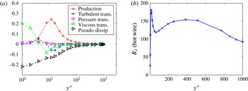
The quality of the data can be judged by computing elementary statistical properties of the flow, such as the mean value,
 $U(y)$
, and by determining the terms involved in the energy budget, which reads, in the steady state (Pope Reference Pope2000),
 $$\begin{eqnarray}-\langle uv\rangle \frac{\text{d}U(y)}{\text{d}y}-\frac{\text{d}}{\text{d}y}\left\langle \frac{1}{2}v\boldsymbol{u}^{2}\right\rangle -\frac{\text{d}}{\text{d}y}\langle vp\rangle -\tilde{\unicode[STIX]{x1D700}}+\unicode[STIX]{x1D708}\frac{\text{d}^{2}k}{\text{d}y^{2}}=0,\end{eqnarray}$$
where
 $\boldsymbol{u}=(u,v,w)$
and
 $p$
are the velocity and pressure fluctuations. The terms in (3.1) are respectively the production term by the mean shear, the turbulent and the pressure transport, the pseudo-dissipation
 $\tilde{\unicode[STIX]{x1D700}}\equiv \unicode[STIX]{x1D708}\langle (\unicode[STIX]{x2202}_{i}u_{j})^{2}\rangle$
and the viscous transport (
 $k$
is the kinetic energy, and depends on the coordinate normal to the wall,
 $y^{+}$
, as does
 $\tilde{\unicode[STIX]{x1D700}}$
). Overall, the terms in (3.1), normalized by
 $u_{\unicode[STIX]{x1D70F}}^{3}/\unicode[STIX]{x1D6FF}_{\unicode[STIX]{x1D708}}$
, shown in figure 1(a) are qualitatively consistent with data shown at lower Reynolds numbers, see, e.g., Pope (Reference Pope2000). We checked that the energy balance equation is satisfied to better than
 $5\times 10^{-3}$
in the dimensionless units used in figure 1(a). We also note that in the so-called log-layer, the two dominant terms in (3.1) are the production terms by the mean shear,
 $-\langle uv\rangle (\text{d}U(y)/\text{d}y)$
, and the pseudo-dissipation term,
 $\tilde{\unicode[STIX]{x1D700}}$
.
Characterization of the flow. (a) The various terms in the equation of production of kinetic energy in (3.1) as a function of the distance from the wall,
 $y^{+}$
, all made dimensionless by dividing by
 $u_{\unicode[STIX]{x1D70F}}^{3}/\unicode[STIX]{x1D6FF}_{\unicode[STIX]{x1D708}}$
. The sum of all of the terms is less than
 $5\times 10^{-3}$
in the dimensionless units used in the code. (b) The Reynolds number, as deduced from measurement of the streamwise velocity fluctuations, see the text, shows a plateau in the range
 $200\lesssim y^{+}\lesssim 650$
.

The intensity of turbulence in homogeneous isotropic flow is characterized by the Reynolds number based on the Taylor microscale. This quantity can be expressed in terms of the longitudinal velocity,
 $u$
, and its derivative with respect to the streamwise coordinate
 $x$
, which can both be determined experimentally using hot wire anemometry:
 $R_{\unicode[STIX]{x1D706}}=\langle u^{2}\rangle /(\unicode[STIX]{x1D708}\langle (\unicode[STIX]{x2202}_{x}u)^{2}\rangle ^{1/2})$
. This definition has also been used in THSF (Garg & Warhaft Reference Garg and Warhaft1998; Shen & Warhaft Reference Shen and Warhaft2000). Figure 1(b) shows the corresponding value of the Reynolds number
 $R_{\unicode[STIX]{x1D706}}$
as a function of
 $y^{+}$
. Consistent with Vreman & Kuerten (Reference Vreman and Kuerten2014) we find that the Reynolds number determined in this way shows a sharp peak close to the wall, where the flow is very anisotropic, and a broad plateau for
 $200\lesssim y^{+}\lesssim 650$
, with a value of
 $R_{\unicode[STIX]{x1D706}}$
larger than
 ${\approx}140$
. The results shown in figure 1(b) are generally consistent with those of Vreman & Kuerten (Reference Vreman and Kuerten2014), obtained at
 $R_{\unicode[STIX]{x1D70F}}\approx 590$
, with a slightly smaller value of
 $R_{\unicode[STIX]{x1D706}}$
(
 $R_{\unicode[STIX]{x1D706}}\approx 100$
) than the one found here. In qualitative agreement with Vreman & Kuerten (Reference Vreman and Kuerten2014), we find that the value of
 $R_{\unicode[STIX]{x1D706}}$
based on the fluctuations of the streamwise velocity is higher than the one obtained by using a definition of
 $R_{\unicode[STIX]{x1D706}}$
based on
 $\langle \boldsymbol{u}^{2}\rangle$
and
 $\langle \unicode[STIX]{x1D74E}^{2}\rangle$
as if the flow were isotropic.
4 Small-scale anisotropy
4.1 Alignment of the vorticity and rate of strain tensor with the flow directions
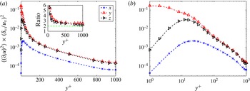
It has been documented that the properties of the flow measured by the second moments of the velocity derivatives tend to become isotropic (Saddoughi & Veeravalli Reference Saddoughi and Veeravalli1994). Isotropy implies that the second moments of the derivatives of
 $\unicode[STIX]{x2202}_{x_{i}}u$
satisfy
 $\langle (\unicode[STIX]{x2202}_{y}u)^{2}\rangle \approx \langle (\unicode[STIX]{x2202}_{z}u)^{2}\rangle \approx 2\langle (\unicode[STIX]{x2202}_{x}u)^{2}\rangle$
. While this property does not have any reason to hold very close to the wall, it tends to become better satisfied when the value of
 $y^{+}$
increases, away from the wall; see figure 2. In particular, the ratios
 $\langle (\unicode[STIX]{x2202}_{y}u)^{2}\rangle /\langle (\unicode[STIX]{x2202}_{x}u)^{2}\rangle$
and
 $\langle (\unicode[STIX]{x2202}_{z}u)^{2}\rangle /\langle (\unicode[STIX]{x2202}_{x}u)^{2}\rangle$
decay from a value
 ${\approx}2.9$
when
 $y^{+}=192$
to a value
 ${\approx}2.35$
at the centre of the channel; see the inset of figure 2(a).
Even at the level of second moments, however, the TCF still shows signs of anisotropy away from the wall, in the log-layer (
 $y^{+}\gtrsim 200$
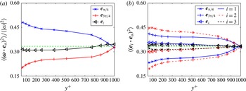
). Such a manifestation can be clearly seen by measuring the moments of vorticity
 $\langle \unicode[STIX]{x1D714}_{i}\unicode[STIX]{x1D714}_{j}\rangle$
. In THSF, it is found that the component of vorticity in the direction
 $\boldsymbol{e}_{\unicode[STIX]{x03C0}/4}=(\boldsymbol{e}_{x}+\boldsymbol{e}_{y})/\sqrt{2}$
(at an angle
 $\unicode[STIX]{x03C0}/4$
in the
 $(x,y)$
plane) is significantly larger than the component of vorticity in the direction
 $\boldsymbol{e}_{3\unicode[STIX]{x03C0}/4}=(\boldsymbol{e}_{y}-\boldsymbol{e}_{x})/\sqrt{2}$
(at an angle
 $3\unicode[STIX]{x03C0}/4$
in the
 $(x,y)$
plane); the ratio between the two decreases as the Reynolds number increases (Pumir Reference Pumir1996). The corresponding quantities
 $\langle (\unicode[STIX]{x1D74E}\boldsymbol{\cdot }\boldsymbol{e}_{\unicode[STIX]{x03C0}/4})^{2}\rangle$
and
 $\langle (\unicode[STIX]{x1D74E}\boldsymbol{\cdot }\boldsymbol{e}_{3\unicode[STIX]{x03C0}/4})^{2}\rangle$
in the log-layer of the TCF are shown in figure 3. For
 $y^{+}\gtrsim 200$
, the ratio between the two quantities is comparable to what was found in turbulent shear flows at comparable Reynolds numbers; it decreases from
 ${\approx}1.87$
at
 $y^{+}=192$
down to
 ${\approx}1.66$
at
 $y^{+}=512$
, to a value close to 1 at the centre of the channel. It should be noted that close to the wall
 $\unicode[STIX]{x1D714}$
is strongly aligned with the spanwise (
 $z$
) direction, even more pronounced than the alignments shown in figure 3(a).
The second moments of the derivatives of the streamwise velocity, along the coordinates in the streamwise (crosses), normal (upper pointing triangles) and spanwise (right pointing triangles) directions, as a function of the distance from the wall,
 $y^{+}$
; (a) linear scale of
 $y^{+}$
and (b) logarithmic scale of
 $y^{+}$
. The ratios
 $\langle (\unicode[STIX]{x2202}_{y}u)^{2}\rangle /\langle (\unicode[STIX]{x2202}_{x}u)^{2}\rangle$
and
 $\langle (\unicode[STIX]{x2202}_{z}u)^{2}\rangle /\langle (\unicode[STIX]{x2202}_{x}u)^{2}\rangle$
, shown in the inset of (a), decrease towards 2 towards the centre of the channel.

Another characterization of the small-scale properties of the flow involves the rate of strain tensor,
 $\unicode[STIX]{x1D64E}$
, defined by
 $\unicode[STIX]{x1D61A}_{ij}=(\unicode[STIX]{x2202}_{i}u_{j}+\unicode[STIX]{x2202}_{j}u_{i})/2$
. As
 $\unicode[STIX]{x1D64E}$
is a symmetric matrix, it has three real eigenvalues, denoted by
 $\unicode[STIX]{x1D706}_{i}$
, which are sorted here in decreasing order:
 $\unicode[STIX]{x1D706}_{1}\geqslant \unicode[STIX]{x1D706}_{2}\geqslant \unicode[STIX]{x1D706}_{3}$
. The incompressibility constraint imposes that
 $\unicode[STIX]{x1D706}_{1}+\unicode[STIX]{x1D706}_{2}+\unicode[STIX]{x1D706}_{3}=0$
. The associated eigenvectors of
 $\unicode[STIX]{x1D64E}$
are denoted as
 $\boldsymbol{e}_{i}$
, with
 $i=1$
, 2 and 3, and
 $|\boldsymbol{e}_{i}|=1$
. Isotropy implies that the eigenvectors
 $\boldsymbol{e}_{i}$
should not show any particular alignment with the flow direction. As was the case for the vorticity, we also find a preferential alignment of the eigenvalues of strain with the directions of the flow. In particular, we find that in the log-layer (
 $y^{+}\gtrsim 200$
), the eigenvector corresponding to the largest eigenvalue of
 $\unicode[STIX]{x1D64E}$
preferentially aligns with
 $\boldsymbol{e}_{3\unicode[STIX]{x03C0}/4}$
, whereas the intermediate eigenvector
 $\boldsymbol{e}_{2}$
preferentially aligns with
 $\boldsymbol{e}_{\unicode[STIX]{x03C0}/4}$
. In comparison, the third eigenvector
 $\boldsymbol{e}_{3}$
does not show a strong alignment with any of the flow directions. We will return to these properties in § 6.
Thus, although the study of the partial derivatives
 $\unicode[STIX]{x2202}_{i}u$
suggests that the flow is close to isotropy, the conclusion of this subsection is that at the Reynolds number of the flow, the vorticity and strain are aligned with some particular directions of the flow, in particular with
 $\boldsymbol{e}_{\unicode[STIX]{x03C0}/4}$
and
 $\boldsymbol{e}_{3\unicode[STIX]{x03C0}/4}$
.
Alignment of the vorticity (a) and of the eigenvectors of strain
 $\unicode[STIX]{x1D64E}$
(b) with the direction of the flow. The strongest alignments of vorticity and strain are with the directions
 $\boldsymbol{e}_{\unicode[STIX]{x03C0}/4}=(\boldsymbol{e}_{x}+\boldsymbol{e}_{y})/\sqrt{2}$
and
 $\boldsymbol{e}_{3\unicode[STIX]{x03C0}/4}=(\boldsymbol{e}_{y}-\boldsymbol{e}_{x})/\sqrt{2}$
. (a) The component of vorticity in the direction
 $\boldsymbol{e}_{\unicode[STIX]{x03C0}/4}$
is significantly larger than in the direction
 $\boldsymbol{e}_{3\unicode[STIX]{x03C0}/4}$
, but isotropy is restored at the centre. (b) The eigenvector corresponding to the intermediate eigenvalue of
 $\unicode[STIX]{x1D64E}$
,
 $\boldsymbol{e}_{2}$
, is preferentially aligned with
 $\boldsymbol{e}_{\unicode[STIX]{x03C0}/4}$
, whereas the eigenvector
 $\boldsymbol{e}_{1}$
is preferentially aligned with
 $\boldsymbol{e}_{3\unicode[STIX]{x03C0}/4}$
. In comparison,
 $\boldsymbol{e}_{3}$
does not show any particular alignment with the flow directions.

4.2 Third moment of
 $\unicode[STIX]{x2202}_{y}u$

We consider here the third moment of the derivative of
 $u$
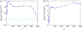
with respect to the normal direction, which in THSF turned out to be very sensitive to the anisotropy resulting from the mean flow. In TCF, we also find a strong value of the third moment, as is illustrated in figure 4(a), which shows the normalized third moment of
 $\unicode[STIX]{x2202}_{y}u$
, the skewness, defined as
 $S_{\unicode[STIX]{x2202}_{y}u}=\langle (\unicode[STIX]{x2202}_{y}u)^{3}\rangle /\langle (\unicode[STIX]{x2202}_{y}u)^{2}\rangle ^{3/2}$
, as a function of the distance from the wall. The main observation is that the skewness is approximately constant, and equal to
 ${\approx}1.07$
(see the dot-dashed line in figure 4
a), from
 $200\lesssim y^{+}\lesssim 750$
. At the centre of the channel,
 $y^{+}\approx 1000$
, the skewness goes to 0, which is a consequence of the symmetry at this particular point. In contrast, a much higher value of the skewness is observed at
 $y^{+}\approx 30$
, in the so-called buffer layer, where the flow is notoriously very far from isotropy. For comparison, the normalized fourth moment of
 $\unicode[STIX]{x2202}_{y}u$
, the flatness, shown in figure 4(b), increases slightly from the beginning of the log-layer up to the centre of the channel.
We note that the properties of the moments of
 $\unicode[STIX]{x2202}_{y}u$
are very similar to those of the moments of the spanwise component of the vorticity,
 $\unicode[STIX]{x1D714}_{z}=(\unicode[STIX]{x2202}_{x}v-\unicode[STIX]{x2202}_{y}u)$
. In particular, the skewness
 $S_{\unicode[STIX]{x1D714}_{z}}\equiv \langle \unicode[STIX]{x1D714}_{z}^{3}\rangle /\langle \unicode[STIX]{x1D714}_{z}^{2}\rangle ^{3/2}$
is approximately constant in the range
 $200\lesssim y^{+}\lesssim 750$
, corresponding to a value
 $S_{\unicode[STIX]{x1D714}_{z}}\approx -0.85$
.
It is interesting to contrast the values of the skewness of
 $\unicode[STIX]{x2202}_{y}u$
and
 $\unicode[STIX]{x1D714}_{z}$
obtained in previous DNS calculations (Pumir & Shraiman Reference Pumir and Shraiman1995; Pumir Reference Pumir1996) or experimental studies of THSF (Garg & Warhaft Reference Garg and Warhaft1998; Shen & Warhaft Reference Shen and Warhaft2000). At small Reynolds numbers (
 $R_{\unicode[STIX]{x1D706}}\lesssim 100$
), achieved in previously published DNS at limited spatial resolution (Pumir & Shraiman Reference Pumir and Shraiman1995; Pumir Reference Pumir1996), the values of the skewness of
 $\unicode[STIX]{x2202}_{y}u$
and
 $\unicode[STIX]{x1D714}_{z}$
are observed to be approximately constant, of the order of 0.84 and
 $-0.55$
respectively. At higher Reynolds numbers accessed experimentally, the skewness of
 $\unicode[STIX]{x2202}_{y}u$
is found to decrease from values of
 ${\approx}0.8$
at
 $R_{\unicode[STIX]{x1D706}}\approx 100$
, with a power law dependence on the Reynolds number
 $S_{\unicode[STIX]{x2202}_{y}u}\propto R_{\unicode[STIX]{x1D706}}^{-1/2}$
. The skewness of
 ${\approx}0.65$
that we find in the DNS of the THSF at
 $R_{\unicode[STIX]{x1D706}}=145$
is consistent with this law. The values obtained in the case of turbulent channel flow are certainly higher than those observed in THSF (see also § 7).
The third (a) and fourth (b) moments of
 $\unicode[STIX]{x2202}_{y}u$
, normalized by its root mean square. The normalized third moment (the skewness) is approximately constant over most of the channel, starting at
 $y^{+}\approx 200$
, which is at the beginning of the log-layer, up to approximately
 $3/4$
of the overall channel width. The value indicated by the horizontal dashed–dotted line is 1.07. The skewness returns to 0 at the centre of the channel (
 $y^{+}\approx 1000$
). The normalized fourth moment (the flatness) slightly increases over the same range of values of
 $y^{+}$
, and goes to a constant
 ${\approx}11$
at the centre of the channel.

4.3 Probability distribution functions of
$\unicode[STIX]{x2202}_{y}u$
and gradient expulsion

The skewness and the flatness of
 $\unicode[STIX]{x2202}_{y}u$
shown in figure 4 indicate that the probability distribution functions (PDFs) of
 $\unicode[STIX]{x2202}_{y}u$
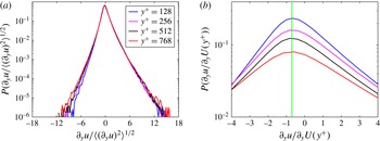
have extended tails, and exhibit a strong asymmetry. This can be directly seen in figure 5(a), which shows the PDF of
 $\unicode[STIX]{x2202}_{y}u$
, normalized by
 $\langle (\unicode[STIX]{x2202}_{y}u)^{2}\rangle ^{1/2}$
, at several values of the distance from the wall, in the range
 $128\leqslant y^{+}\leqslant 768$
. The positive tails of the PDFs vary only slightly as a function of the distance from the wall in the range shown, whereas the negative tails tend to extend further when
 $y^{+}$
increases.
All of the PDFs shown in figure 5(a) peak at values of
 $\unicode[STIX]{x2202}_{y}u$
smaller than 0, a situation reminiscent of what was observed in THSF (Pumir & Shraiman Reference Pumir and Shraiman1995; Pumir Reference Pumir1996), and for the scalar. In quantitative terms, it was found that the PDF of
 $\unicode[STIX]{x2202}_{y}u$
peaked at a value
 $\unicode[STIX]{x2202}_{y}u\approx -0.6S$
, where
 $S$
is the mean shear. Figure 5(b) shows the PDF of
 $\unicode[STIX]{x2202}_{y}u$
, divided by the mean velocity gradient
 $U^{\prime }(y^{+})$
, blown up near
 $\unicode[STIX]{x2202}_{y}u=0$
. The maximum of the curves is observed to peak at a value of
 ${\approx}-0.7$
, slightly higher than observed in THSF. Even though
 $U^{\prime }(y^{+})\sim 1/y^{+}$
, all curves peak at the same point in rescaled units.
The PDFs of the derivative
 $\unicode[STIX]{x2202}_{y}u$
at several locations away from the wall and from the centre:
 $128\leqslant y^{+}\leqslant 768\approx 3h/4$
. The PDFs normalized by the root mean square of the fluctuating quantities (a) superpose very well, except at
 $y^{+}=128$
, where the probability of observing large negative fluctuations is smaller than at larger values of
 $y^{+}$
. The PDFs normalized by the mean gradient
 $U^{\prime }(y)$
(b) show that the PDFs of
 $\unicode[STIX]{x2202}_{y}u$
peak at a value
 ${\approx}-0.7U^{\prime }$
. This can be interpreted as a partial expulsion of the gradient, more significant than what has been observed in THSF.

The peak of the PDF of
 $\unicode[STIX]{x2202}_{y}u$
at a value close to
 ${\approx}-0.7U^{\prime }(y^{+})$
implies that the derivative with respect to the distance from the wall of the streamwise velocity component,
 $\unicode[STIX]{x2202}_{y}(U+u)$
, has its largest probability at a value that is significantly reduced compared with the mean gradient
 $U^{\prime }(y^{+})$
.
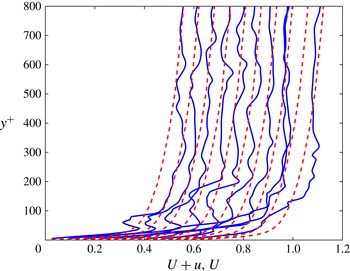
In the problem of a passive scalar with a mean gradient, the PDF of the scalar gradient strongly peaks at 0 (Holzer & Siggia Reference Holzer and Siggia1994; Pumir Reference Pumir1994; Tong & Warhaft Reference Tong and Warhaft1994). This corresponds to the simple physical picture of a scalar field approximately constant over large domains of the flow, from which the gradient is ‘expelled’. These regions are separated by narrow cliffs, where strong scalar variations concentrate (Holzer & Siggia Reference Holzer and Siggia1994; Pumir Reference Pumir1994). A similar, although weaker, expulsion mechanism was observed in the case of THSF (Pumir & Shraiman Reference Pumir and Shraiman1995; Pumir Reference Pumir1996). In TCF, a similar phenomenon can be observed, as illustrated in figure 6, which shows the instantaneous velocity profile at several locations along the streamwise direction (
 $x$
), in a given
 $(x,y)$
plane, corresponding to a fixed spanwise location. The full curves show the actual velocity profile
 $U(y)+u(x,y)$
as a function of
 $y$
(vertical), the curves corresponding to different values of
 $x$
being shifted by a quantity proportional to
 $x$
. For comparison, the dashed curves show the mean velocity profile, which is independent of
 $x$
in the fully developed channel flow considered here, shifted by the same quantity as the instantaneous velocity. Figure 6 thus suggests the existence of regions with a streamwise velocity close to constant, separated by steep cliffs. The sharpest one in figure 6 is found at a value
 $y^{+}\approx 200$
, while smaller ones are visible at different distances from the wall. These structures are comparable to those presented in the case of homogeneous shear flows (Pumir & Shraiman Reference Pumir and Shraiman1995; Pumir Reference Pumir1996). We stress that figure 6 provides a physical illustration of the quantitative observations concerning the distribution of
 $\unicode[STIX]{x2202}_{y}u$
.
Snapshot of the instantaneous velocity profile, at a particular instant of time, in an
 $(x,y)$
plane. The full lines show the velocity,
 $U+u$
. For comparison, the dashed lines show the mean velocity profile as a function of
 $y$
. The cliff and ramp structure is visible, as it was visible in TSHF (Pumir & Shraiman Reference Pumir and Shraiman1995; Pumir Reference Pumir1996). Two consecutive traces are separated by
 $\unicode[STIX]{x0394}x=2\unicode[STIX]{x03C0}/100$
.

5 Invariants of the velocity gradient tensors and implications for turbulent production
While the results presented in § 4 show a strong anisotropy of the velocity field, other characterizations of the TCF flow involving scalar combinations of velocity gradients are remarkably similar to HIT. We define the velocity gradient
 $\unicode[STIX]{x1D608}_{ij}=\unicode[STIX]{x2202}_{i}u_{j}$
and its decomposition into strain and vorticity,
 $\unicode[STIX]{x1D608}_{ij}=\unicode[STIX]{x1D61A}_{ij}-\unicode[STIX]{x1D716}_{ijk}\unicode[STIX]{x1D714}_{k}/2$
. We begin with two examples that we understand analytically.
5.1 Second- and third-order invariants of the velocity gradient tensor
In homogeneous flows, the two quantities
 $A_{2}\equiv \langle \unicode[STIX]{x1D608}_{ij}\unicode[STIX]{x1D608}_{ji}\rangle$
and
 $A_{3}\equiv \langle \unicode[STIX]{x1D608}_{ij}\unicode[STIX]{x1D608}_{jk}\unicode[STIX]{x1D608}_{ki}\rangle$
are known to be identically 0 (Betchov Reference Betchov1956). Using the fact that
 $A_{2}=\langle \text{tr}(\unicode[STIX]{x1D64E}^{2})\rangle -\langle \unicode[STIX]{x1D74E}^{2}\rangle /2$
and
 $A_{3}=\langle \text{tr}(\unicode[STIX]{x1D64E}^{3})\rangle +3/4\langle \unicode[STIX]{x1D74E}\boldsymbol{\cdot }\unicode[STIX]{x1D64E}\boldsymbol{\cdot }\unicode[STIX]{x1D74E}\rangle$
, these relations provide kinematic constraints between strain and vorticity and between strain skewness and vortex stretching,
 $\langle \unicode[STIX]{x1D74E}\boldsymbol{\cdot }\unicode[STIX]{x1D64E}\boldsymbol{\cdot }\unicode[STIX]{x1D74E}\rangle$
. In a highly inhomogeneous case, such as a turbulent boundary layer, it may be expected that
 $A_{2}$
and
 $A_{3}$
deviate significantly from 0. A deviation from
 $A_{2}=0$
would indicate an imbalance between strain and vorticity, whereas a deviation from
 $A_{3}=0$
would point to a difference between vortex stretching,
 $\langle \unicode[STIX]{x1D74E}\boldsymbol{\cdot }\unicode[STIX]{x1D64E}\boldsymbol{\cdot }\unicode[STIX]{x1D74E}\rangle$
, and the strain skewness,
 $\langle \text{tr}(\unicode[STIX]{x1D64E}^{3})\rangle$
.
We determined numerically the values of
 $A_{2}$
and
 $A_{3}$
as a function of
 $y^{+}$
, and found that both
 $A_{2}$
and
 $A_{3}$
are remarkably small throughout the entire width of the channel. In quantitative terms,
 $A_{2}$
is negative for
 $y^{+}\lesssim 16$
, and positive otherwise. The most negative value of
 $A_{2}/\langle \text{tr}(\unicode[STIX]{x1D64E}^{2})\rangle$
is
 ${\approx}-0.06$
(for
 $y^{+}\approx 5$
) and the most positive value is
 ${\approx}0.025$
(for
 $y^{+}\approx 32$
). Similarly, the value of
 $A_{3}$
is positive for
 $y^{+}\lesssim 10$
and negative otherwise; its magnitude is smaller than
 ${\approx}6\,\%$
of the magnitude of
 $\langle \text{tr}(\unicode[STIX]{x1D64E}^{3})\rangle$
.
It follows from these results that the relations known to hold in homogeneous turbulence,
 $\langle \text{tr}(\unicode[STIX]{x1D64E}^{2})\rangle =\langle \unicode[STIX]{x1D74E}^{2}\rangle /2$
and
 $\langle \text{tr}(\unicode[STIX]{x1D64E}^{3})\rangle =-3/4\langle \unicode[STIX]{x1D74E}\boldsymbol{\cdot }\unicode[STIX]{x1D64E}\boldsymbol{\cdot }\unicode[STIX]{x1D74E}\rangle$
, are very nearly satisfied in the turbulent channel flow. The first of these relations was already noted to hold approximately in TCF by Bradshaw & Perot (Reference Bradshaw and Perot1993), where they showed that
 $A_{2}=\unicode[STIX]{x2202}^{2}\langle v^{2}\rangle /\unicode[STIX]{x2202}y^{2}$
.
As the variations of mean quantities are typically much smaller than averages of the gradients of fluctuating fields,
 $A_{2}$
is effectively much smaller than
 $\langle \text{tr}(\unicode[STIX]{x1D64E}^{2})\rangle$
. Similarly, elementary algebra shows that the third moment
 $A_{3}$
can be expressed as
 $A_{3}=(1/2)\unicode[STIX]{x2202}^{3}\langle v^{3}\rangle /\unicode[STIX]{x2202}y^{3}-(3/2)\unicode[STIX]{x2202}\langle v\text{tr}(\unicode[STIX]{x1D63C}^{2})\rangle /\unicode[STIX]{x2202}y$
, thus explaining the numerical observation that
 $A_{3}$
is much smaller than
 $\langle \text{tr}(\unicode[STIX]{x1D64E}^{3})\rangle$
.
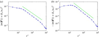
The averages
 $\langle \text{tr}(\unicode[STIX]{x1D64E}^{2})\rangle$
(a) and
 $\langle \text{tr}(\unicode[STIX]{x1D64E}^{3})\rangle$
(b) as a function of the distance from the wall,
 $y^{+}$
. The two quantities decay with an approximate power law away from the wall, for
 $30\lesssim y^{+}\lesssim 500$
. The straight lines correspond to power laws with exponents
 $-1.14$
(a) and
 $-1.5$
(b). As a result, the dimensionless ratio
 $\langle \text{tr}(\unicode[STIX]{x1D64E}^{3})\rangle /\langle \text{tr}(\unicode[STIX]{x1D64E}^{2})\rangle ^{3/2}$
slightly increases away from the wall.

As explained in Bradshaw & Perot (Reference Bradshaw and Perot1993), the significance of the small value of
 $A_{2}$
is that the kinetic energy dissipation term can be expressed equivalently in terms of
 $\langle \unicode[STIX]{x1D74E}^{2}\rangle$
or in terms of the strain
 $\langle \text{tr}(\unicode[STIX]{x1D64E}^{2})\rangle$
, up to very small corrections. Similarly, the small value of
 $A_{3}$
implies that the overall production of velocity gradients by turbulence can be expressed equivalently in terms of vortex stretching,
 $\langle \unicode[STIX]{x1D74E}\boldsymbol{\cdot }\unicode[STIX]{x1D64E}\boldsymbol{\cdot }\unicode[STIX]{x1D74E}\rangle$
, or in terms of the third moment of
 $\unicode[STIX]{x1D64E}$
,
 $\langle \text{tr}(\unicode[STIX]{x1D64E}^{3})\rangle$
. This is a direct consequence of the Navier–Stokes equations, which lead to the following expression for the production of velocity gradients,
 $\sum _{i,j=1}^{3}(\unicode[STIX]{x2202}_{i}u_{j})^{2}=\text{tr}(\unicode[STIX]{x1D63C}\boldsymbol{\cdot }\unicode[STIX]{x1D63C}^{\text{T}})$
:
 $$\begin{eqnarray}\frac{\text{d}}{\text{d}t}\langle \unicode[STIX]{x1D63C}\boldsymbol{\cdot }\unicode[STIX]{x1D63C}^{\text{T}}\rangle +2\langle \text{tr}(\unicode[STIX]{x1D63C}^{2}\unicode[STIX]{x1D63C}^{\text{T}})\rangle =\text{RHS},\end{eqnarray}$$
where the
 $\text{RHS}$
term contains contributions from viscosity (dissipation), pressure, transport by the fluctuations and interaction with the mean flow (Pope Reference Pope2000). Away from the wall region, for
 $y^{+}\gtrsim 100$
, the nonlinear term in (5.1) dominates over all of the other contributions (Pope Reference Pope2000; Vreman & Kuerten Reference Vreman and Kuerten2014). Therefore, using the relation
 $\langle \text{tr}(\unicode[STIX]{x1D63C}^{3})\rangle \approx 0$
, one obtains for
 $y^{+}\gtrsim 100$
the following approximate relation
 $\langle \text{tr}(\unicode[STIX]{x1D63C}^{2}\unicode[STIX]{x1D63C}^{\text{T}})\rangle \approx -\langle \unicode[STIX]{x1D74E}\boldsymbol{\cdot }\unicode[STIX]{x1D64E}\boldsymbol{\cdot }\unicode[STIX]{x1D74E}\rangle \approx (4/3)\langle \text{tr}(\unicode[STIX]{x1D64E}^{3})\rangle$
. This in turn leads to the conclusion that away from the wall, small-scale production is expressed in terms of vortex stretching, as is the case in homogeneous isotropic flows.
Figure 7 shows the second and third moments of
 $\unicode[STIX]{x1D64E}$
as a function of the distance from the wall. We observe that, as was the case in homogeneous isotropic flows, the moment
 $\langle \text{tr}(\unicode[STIX]{x1D64E}^{3})\rangle$
is negative, which is related to the positive sign of vortex stretching,
 $\langle \unicode[STIX]{x1D74E}\boldsymbol{\cdot }\unicode[STIX]{x1D64E}\boldsymbol{\cdot }\unicode[STIX]{x1D74E}\rangle >0$
. We find that both
 $\langle \text{tr}(\unicode[STIX]{x1D64E}^{2})\rangle$
and
 $-\langle \text{tr}(\unicode[STIX]{x1D64E}^{3})\rangle$
have approximate power law dependences in the log-layer, with power laws close to
 ${y^{+}}^{\unicode[STIX]{x1D6FC}_{2}}$
and
 ${y^{+}}^{\unicode[STIX]{x1D6FC}_{3}}$
for the second and third moments respectively. The exponent
 $\unicode[STIX]{x1D6FC}_{3}$
is very close to
 $-3/2$
; see figure 7(b). The data shown in figure 7(a) suggest a value of
 $\unicode[STIX]{x1D6FC}_{2}$
close to
 $-1$
:
 $\unicode[STIX]{x1D6FC}_{2}\approx -1.14$
. In general, the exponents
 $\unicode[STIX]{x1D6FC}_{2}$
and
 $\unicode[STIX]{x1D6FC}_{3}$
can be approximately estimated by using the relation
 $\tilde{\unicode[STIX]{x1D700}}\approx u_{\unicode[STIX]{x1D70F}}^{3}/y^{+}$
, which can be deduced by balancing the dissipation
 $\tilde{\unicode[STIX]{x1D700}}$
with the production term
 $U^{\prime }(y)\times \langle uv\rangle$
(see Brouwers Reference Brouwers2007). As a result, the dimensionless ratio
 $\langle \text{tr}(\unicode[STIX]{x1D64E}^{3})\rangle /\langle \text{tr}(\unicode[STIX]{x1D64E}^{2})\rangle ^{3/2}$
is approximately constant for
 $y^{+}\gtrsim 20$
, up to the centre of the channel (with a small decrease from
 ${\approx}-0.25$
in the buffer layer to
 ${\approx}-0.32$
at the centre). These values are generally consistent with the value of
 $\langle \text{tr}(\unicode[STIX]{x1D64E}^{3})\rangle /\langle \text{tr}(\unicode[STIX]{x1D64E}^{2})\rangle ^{3/2}$
in HIT, where this dimensionless ratio is equal to
 $(7/4)(2/15)^{1/2}S_{\unicode[STIX]{x2202}_{x}u_{x}}$
, with
 $S_{\unicode[STIX]{x2202}_{x}u_{x}}=\langle (\unicode[STIX]{x2202}_{x}u_{x})^{3}\rangle /\langle (\unicode[STIX]{x2202}_{x}u_{x})^{2}\rangle ^{3/2}$
being of the order of 0.5, which equals that in the centre of the channel to a few per cent.
The results in this subsection suggest that the anisotropy that is very visible at the level of the derivative
 $\unicode[STIX]{x2202}_{y}u$
does not much affect the second- and third-order moments which are invariant under rotations (this is consistent with the results of Cardesa et al. (Reference Cardesa, Mistry, Gan and Dawson2013)). This may be related to the observation that the third moment
 $\langle (\unicode[STIX]{x2202}_{y}u)^{3}\rangle$
does not enter any of the expressions of the low-order moments considered here.
5.2 Higher-order invariants
In homogeneous and isotropic turbulence, the fourth-order velocity tensor can be fully characterized by four independent quantities that are explicitly invariant under rotation (Siggia Reference Siggia1981):
 $$\begin{eqnarray}\left.\begin{array}{@{}c@{}}I_{1}=\langle \text{tr}(\unicode[STIX]{x1D64E}^{2})^{2}\rangle ,\\ I_{2}=\langle (\unicode[STIX]{x1D74E}^{2})\text{tr}(\unicode[STIX]{x1D64E}^{2})\rangle ,\\ I_{3}=\langle \unicode[STIX]{x1D74E}\boldsymbol{\cdot }\unicode[STIX]{x1D64E}^{2}\boldsymbol{\cdot }\unicode[STIX]{x1D74E}\rangle ,\\ I_{4}=\langle (\unicode[STIX]{x1D74E}^{2})^{2}\rangle .\end{array}\right\}\end{eqnarray}$$
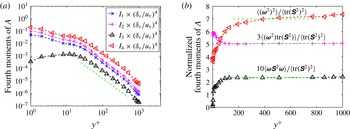
These invariants are shown in figure 8 for TCF. The dependence of the fourth-order moments
 $I_{1},\ldots ,I_{4}$
as a function of the distance from the wall,
 $y^{+}$
, is shown in figure 8(a). Away from the wall region, for
 $y^{+}\gtrsim 20$
, the dependence of the fourth-order invariants on
 $y^{+}$
is very close to a power law with an exponent
 $-2.1$
, approximately valid for
 $20\lesssim y^{+}\lesssim 700$
. This is again close to the value of
 $-2$
expected for
 $\tilde{\unicode[STIX]{x1D700}}^{2}$
. Figure 8(b) shows three ratios formed by normalizing with
 $I_{1}$
. The ratios
 $I_{2}/I_{1}$
and
 $I_{3}/I_{1}$
are both essentially constant over a wide range of values of
 $y^{+}$
, and equal respectively to
 ${\approx}1.68$
and
 ${\approx}0.235$
. In comparison, the ratio
 $I_{4}/I_{1}$
increases slightly throughout the entire width of the channel. The value indicated in figure 8(b) is equal to 7. The values of the ratios
 $I_{2}/I_{1}$
and
 $I_{3}/I_{1}$
are fully consistent with the values reported for HIT (Ishihara et al.
Reference Ishihara, Kaneda, Yokokawa, Itakura and Uno2007):
 $I_{2}/I_{1}\approx 1.75$
,
 $I_{3}/I_{1}\approx 0.230$
. The value found in HIT,
 $I_{4}/I_{1}\approx 8$
, is slightly larger than the value found in the channel flow. We also mention that the values of the ratios between the fourth-order moments of the velocity gradient tensor in THSF at
 $R_{\unicode[STIX]{x1D706}}\approx 145$
are completely consistent with the values obtained in the log-layer of TCF.
The invariant fourth moments of the velocity gradient tensor. (a) Variation with the distance from the wall of the four invariants defined by (5.2), normalized by
 $(u_{\unicode[STIX]{x1D70F}}/\unicode[STIX]{x1D6FF}_{\unicode[STIX]{x1D708}})^{4}$
. Aside from the region close to the wall, where
 $I_{3}$
is much smaller than the other moments, the moments all decay, with a decay law close to
 ${y^{+}}^{-2}$
, indicated by the dashed line. (b) The ratios
 $I_{4}/I_{1}$
,
 $3I_{2}/I_{1}$
and
 $10I_{3}/I_{1}$
. Whereas the ratio
 $I_{4}/I_{1}$
increases throughout the entire width of the channel, the ratios
 $I_{2}/I_{1}$
and
 $I_{3}/I_{1}$
reach approximately constant values, of the order of
 $I_{2}/I_{1}\approx 1.68$
and
 $I_{3}/I_{1}\approx 0.235$
.

Thus, the rotationally invariant fourth moments of the velocity gradient obey simple power laws as a function of
 $y^{+}$
and have ratios very close to the values in HIT or in THSF.
6 Structure of the eigenvalues of the rate of strain matrix
As pointed out by Siggia (Reference Siggia1981), the ratios between the moments up to four of the velocity gradient tensor reflect non-trivial properties of the correlation between the eigenvectors of the rate of strain tensor and vorticity; see also Ashurst et al. (Reference Ashurst, Kerstein, Kerr and Gibson1987), Tsinober (Reference Tsinober2009) and Wallace (Reference Wallace2009). Since we showed in the previous section that the scalar invariants that completely characterize the moments of the velocity gradient tensor in HIT of order four or less are virtually identical in TCF, it is natural to look in more detail at the strain–vorticity correlation, figure 9(a).
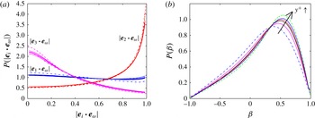
We again find very close similarity between HIT and TCF in the PDFs of the cosines between vorticity and the principal axes of the strain. The vorticity is preferentially along the intermediate eigenvector of the rate of strain, i.e. the weak expanding direction, perpendicular to the compressing direction, and does not show any particular alignment with respect to the strong expanding direction; see figure 9(a). The agreement between HIT and TCF is even very good for
 $y^{+}=64$
, which is not yet in the log-layer. Finally, the observation that
 $\unicode[STIX]{x1D74E}$
aligns with
 $\boldsymbol{e}_{2}$
(see figure 9
a) on one hand and with
 $\boldsymbol{e}_{\unicode[STIX]{x03C0}/4}$
(see figure 3
a) on the other hand points to an alignment between
 $\boldsymbol{e}_{2}$
and
 $\boldsymbol{e}_{\unicode[STIX]{x03C0}/4}$
, which is consistent with the results shown in figure 3(b).
In turbulent flows, the observation that
 $\langle \text{tr}(\unicode[STIX]{x1D64E}^{3})\rangle <0$
is related to an asymmetry in the distribution of the eigenvalues of strain. Namely, using the identity deduced from the condition
 $\unicode[STIX]{x1D706}_{1}+\unicode[STIX]{x1D706}_{2}+\unicode[STIX]{x1D706}_{3}=0$
that
 $\unicode[STIX]{x1D706}_{1}^{3}+\unicode[STIX]{x1D706}_{2}^{3}+\unicode[STIX]{x1D706}_{3}^{3}=3\unicode[STIX]{x1D706}_{1}\unicode[STIX]{x1D706}_{2}\unicode[STIX]{x1D706}_{3}$
, a negative value of
 $\langle \text{tr}(\unicode[STIX]{x1D64E}^{3})\rangle$
imposes that, on average, the probability of having two positive eigenvalues of
 $\unicode[STIX]{x1D64E}$
is higher that the probability of having one positive and two negative eigenvalues; in other words, the intermediate eigenvalue
 $\unicode[STIX]{x1D706}_{2}$
is preferentially positive. A common way to quantify this property consists in introducing a dimensionless quantity
 $\unicode[STIX]{x1D6FD}$
,
 $$\begin{eqnarray}\unicode[STIX]{x1D6FD}=\frac{\sqrt{6}\unicode[STIX]{x1D706}_{2}}{\sqrt{\unicode[STIX]{x1D706}_{1}^{2}+\unicode[STIX]{x1D706}_{2}^{2}+\unicode[STIX]{x1D706}_{3}^{2}}},\end{eqnarray}$$
such that
 $-1\leqslant \unicode[STIX]{x1D6FD}\leqslant 1$
. The tendency of
 $\unicode[STIX]{x1D706}_{2}$
to be preferentially positive leads to an asymmetric PDF of
 $\unicode[STIX]{x1D6FD}$
, as seen many times in simulations of HIT flows.
The PDF of
 $\unicode[STIX]{x1D6FD}$
in the channel flow, shown in figure 9(b), at several values of
 $y^{+}$
in the range
 $64\leqslant y^{+}\leqslant 768$
, and for an HIT flow, demonstrate, as expected, that the values of
 $\unicode[STIX]{x1D6FD}$
are preferentially positive. The changes of the PDF of
 $\unicode[STIX]{x1D6FD}$
when
 $y^{+}$
increases, indicated by the arrow in figure 9(b), are systematic, but moderate, for
 $y^{+}\gtrsim 100$
. The PDF of
 $\unicode[STIX]{x1D6FD}$
at the centre of the channel (not shown) simply extrapolates the trend shown in figure 9(b). The PDF in the HIT case deviates only slightly from the PDFs shown in the log-layer of the channel.
Alignment between the eigenvectors of strain and vorticity (a) and dimensionless eigenvalue
 $\unicode[STIX]{x1D6FD}$
as defined by (6.1) (b). (a) The PDF of the scalar product
 $|\boldsymbol{e}_{i}\boldsymbol{\cdot }\boldsymbol{e}_{\unicode[STIX]{x1D714}}|$
is shown at different values of
 $y^{+}$
. In the range
 $128\leqslant y^{+}\leqslant 768$
, the PDFs are indistinguishable. Deviations from the universal PDFs are visible in the data for
 $y^{+}=64$
shown as dashed-dot curves. The dashed lines show the PDFs for HIT. The difference is small, but visible for
 $|\boldsymbol{e}_{3}\boldsymbol{\cdot }\boldsymbol{e}_{\unicode[STIX]{x1D714}}|$
. The PDFs for
 $|\boldsymbol{e}_{2}\boldsymbol{\cdot }\boldsymbol{e}_{\unicode[STIX]{x1D714}}|$
(
 $|\boldsymbol{e}_{1}\boldsymbol{\cdot }\boldsymbol{e}_{\unicode[STIX]{x1D714}}|$
) almost perfectly superpose with the corresponding PDFs in TCF at
 $y^{+}=64$
(
 $y^{+}\geqslant 128$
). (b) The PDF of
 $\unicode[STIX]{x1D6FD}$
at values of
 $y^{+}=64$
(blue dashed-dot), 128, 256, 512 and 768. The arrow indicates how the PDFs vary as a function of
 $y^{+}$
. In the range
 $y^{+}\gtrsim 200$
, which corresponds to the log-layer, the curves differ only slightly from the curve for the case of HIT, shown as a green dashed line.

7 Discussion and concluding remarks
This article establishes two new facts based on the simulation of TCF available on the Johns Hopkins University Turbulence Database (Li et al. Reference Li, Wan, Yang, Burns, Meneveau, Burns, Chen, Szalay and Eyink2008; Lee et al. Reference Lee, Malaya and Moser2013; Graham et al. Reference Graham, Lee, Malaya, Moser, Eyink and Meneveau2014):
-
(i) the skewness of
$\unicode[STIX]{x2202}_{y}u$
is
${\sim}1.1$
and is constant throughout the log-layer, -
(ii) the rotationally invariant vorticity–strain correlations that characterize HIT are virtually unchanged in the log-layer of TCF.


These facts superficially appear contradictory but may point to potent extensions of the classical phenomenological description of wall-bounded shear flow, and certainly invite experimental tests at higher Reynolds numbers and other geometries. We elaborate each in turn.
The restoration of isotropy is an informative characterization of the turbulence state. Phenomenological considerations, following Kolmogorov (Corrsin Reference Corrsin1958; Lumley Reference Lumley1967), predict that the effect of anisotropy on the velocity derivatives is of the order of the ratio of the large-scale gradient to the gradient at the scale of the smallest eddies, which behaves as
 $R_{\unicode[STIX]{x1D706}}^{-1}$
. This argument correctly predicts how quantities based on the second-order moments of the velocity derivatives return to isotropy at high Reynolds numbers (Pumir & Shraiman Reference Pumir and Shraiman1995; Ishihara, Yoshida & Kaneda Reference Ishihara, Yoshida and Kaneda2002; Tsuji Reference Tsuji2003; Kaneda, Morishita & Ishihara Reference Kaneda, Morishita and Ishihara2013). Passive scalar advection in a shear flow, however, strongly violates standard theory since the derivative skewness is of order 1 (Sreenivasan Reference Sreenivasan1991; Shraiman & Siggia Reference Shraiman and Siggia2000). Therefore, based on an analogy between scalar transport and momentum transport in a shear, Pumir & Shraiman (Reference Pumir and Shraiman1995) simulated THSF and computed
 $S_{\unicode[STIX]{x2202}_{y}u}$
. New simulations following Pumir (Reference Pumir1996) for THSF at
 $R_{\unicode[STIX]{x1D706}}\sim 144$
very close to TCF show
 $S_{\unicode[STIX]{x2202}_{y}u}\approx 0.8$
. Laboratory experiments with active grids provide THSF data up to
 $R_{\unicode[STIX]{x1D706}}\sim 1000$
and suggest
 $S_{\unicode[STIX]{x2202}_{y}u}\propto R_{\unicode[STIX]{x1D706}}^{-1/2}$
, still a violation of phenomenological theory, but consistent with eventual isotropy.
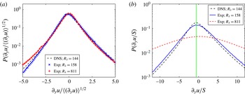
Comparison of the PDF of
 $\unicode[STIX]{x2202}_{y}u$
in THSF between moderate-Reynolds-number DNS (
 $R_{\unicode[STIX]{x1D706}}=144$
, dashed–dotted line) and experiment (
 $R_{\unicode[STIX]{x1D706}}=158$
, crosses (a) or full line (b)) and high-Reynolds-number experiment (
 $R_{\unicode[STIX]{x1D706}}=811$
, plus signs (a) or dashed line (b)). The experimental data come from Shen & Warhaft (Reference Shen and Warhaft2000) and the numerical data come from simulations of THSF. (a) Shows the whole PDF of
 $\unicode[STIX]{x2202}_{y}u$
in units of the root mean square
 $\langle (\unicode[STIX]{x2202}_{y}u)^{2}\rangle ^{1/2}$
. (b) Shows the PDF of
 $\unicode[STIX]{x2202}_{y}u$
in units of the constant imposed mean shear,
 $S=U^{\prime }(y)$
. The vertical line corresponds to
 $\unicode[STIX]{x2202}_{y}u/S=-0.6$
. The partial expulsion, shown at moderate Reynolds numbers
 $R_{\unicode[STIX]{x1D706}}\lesssim 200$
by the peak of the PDF of
 $\unicode[STIX]{x2202}_{y}u$
at
 ${\approx}-0.6S$
, disappears when
 $R_{\unicode[STIX]{x1D706}}$
is much larger. The data shown in this figure are to be compared with the data in TCF, shown at smaller Reynolds numbers in figure 5.

The PDF of
 $\unicode[STIX]{x2202}_{y}u$
around the origin defines the most probable gradient in the flow. For scalar transport, the PDF peaked at minus the mean external gradient, implying the plateau–step structure seen in single-point data traces. In the simulations of THSF, at Reynolds numbers up to
 $R_{\unicode[STIX]{x1D706}}\approx 145$
, the peak of
 $\unicode[STIX]{x2202}_{y}u$
is
 ${\approx}-0.6U^{\prime }$
; see figure 10(b). When we magnified the data from Shen & Warhaft (Reference Shen and Warhaft2000) around the origin, see figure 10, we found the peak in PDF(
 $\unicode[STIX]{x2202}_{y}u$
) at
 $R_{\unicode[STIX]{x1D706}}=158$
to be completely consistent with our numerics, but to move close to 0 at
 $R_{\unicode[STIX]{x1D706}}=811$
. This observation demonstrates a restoration of isotropy of THSF at high enough Reynolds number, consistent with the observed decrease of the skewness of
 $\unicode[STIX]{x2202}_{y}u$
(Shen & Warhaft Reference Shen and Warhaft2000). For the TCF at
 $Re_{\unicode[STIX]{x1D70F}}\approx 1000$
studied here, the skewness of
 $\unicode[STIX]{x2202}_{y}u$
is larger than in THSF at a comparable value of
 $R_{\unicode[STIX]{x1D706}}$
, and constant over the entire log-layer, while the peak in PDF(
 $\unicode[STIX]{x2202}_{y}u$
) is
 ${\approx}-0.7U^{\prime }(y)$
. This is slightly more negative than the value observed for THSF at a comparable
 $R_{\unicode[STIX]{x1D706}}$
, but note that the PDFs for TCF superimpose very well around the origin, even though the mean velocity gradient varies by 6 times over the range of distances from the wall considered; see figure 5.
It is thus very interesting to ask about the behaviour of wall-bounded shear flow at
 $R_{\unicode[STIX]{x1D70F}}$
larger than
 ${\sim}1000$
examined here. One might suppose that the flow will approach isotropy like THSF. A more interesting alternative and not implausible outcome in our view is
 $S_{\unicode[STIX]{x2202}_{y}u}\sim 1$
independent of
 $y$
, and maintained by injection of slowly moving fluid from the wall.
Irrespective of the infinite-Reynolds-number limit, THSF is a useful model for wall-bounded flow, as anticipated by Pumir & Shraiman (Reference Pumir and Shraiman1995) (see also Pumir Reference Pumir1996) and further developed by Cardesa et al. (Reference Cardesa, Vela-Martin, Dong and Jimenez2015), Dong et al. (Reference Dong, Lozano-Durán, Sekimoto and Jimenez2015) and Dong (Reference Dong2016), who observed suggestive analogies between the structures in THSF and those of TCF away from the wall (Theodorsen Reference Theodorsen1952; Moin & Kim Reference Moin and Kim1985; Head & Bandyopadhyay Reference Head and Bandyopadhyay1991; Wu & Moin Reference Wu and Moin2009).
Symmetry restricts the number of independent one-point velocity gradient correlations that collectively define the state of HIT. For the second and third moments only one scalar combination of vorticity and strain is allowed by homogeneity. We generalized the argument of Bradshaw & Perot (Reference Bradshaw and Perot1993) for
 $\langle \text{tr}(\unicode[STIX]{x1D63C}^{2})\rangle$
, and related
 $\langle \text{tr}(\unicode[STIX]{x1D63C}^{3})\rangle$
in TCF to
 $y$
derivatives of averaged quantities that are small. Thus, the third-order scalar combinations of vorticity and strain in TCF behave as if they were homogeneous isotropic, but of course there will be many non-zero gradient correlations in TCF that violate isotropy or reflection invariance. All isotropic combinations of vorticity and strain vary with distance from the wall very nearly as one would infer from their dimension and the relation for the local dissipation,
 $\tilde{\unicode[STIX]{x1D716}}\sim {y^{+}}^{-1}$
(Brouwers Reference Brouwers2007; Kaneda et al.
Reference Kaneda, Morishita and Ishihara2013).
The fourth-order scalar invariants of the velocity–strain correlations are not constrained by homogeneity (Siggia Reference Siggia1981). Their ratios in TCF are nearly independent of
 $y$
and closely approximate the values for HIT or THSF. For HIT there is reasonable evidence that all four invariants scale in the same way with
 $R_{\unicode[STIX]{x1D706}}$
(Ishihara et al.
Reference Ishihara, Kaneda, Yokokawa, Itakura and Uno2007), which also defines the growth in squared dissipation. The observed collapse for
 $100<y_{+}<800$
of the distributions of the angles between vorticity and the rate of strain axes onto universal curves that are very close to those of HIT provides a hint that the statistical properties of the scalar invariants of the velocity gradient tensor of order higher than 4 will be similar to those in HIT.
To rephrase the dichotomy with which we began this section, correlations that violate rotation and reflection invariance such as odd powers of
 $\unicode[STIX]{x2202}_{y}u$
seem to be decoupled from those that are invariant under the full rotation group. Both the Kolmogorov energy cascade and the von Kármán boundary layer are theories built around a conserved flux with a scaling regime sandwiched between large and small scales (Tennekes & Lumley Reference Tennekes and Lumley1983). In the related problem of a passive scalar mixed by a turbulent flow, the generation of small scales in the presence of a passive scalar flux leads to a natural decomposition of the moments of the scalar gradient in terms of decomposition of the rotation group
 $SO(3)$
(Mydlarski et al.
Reference Mydlarski, Pumir, Shraiman, Siggia and Warhaft1998; Shraiman & Siggia Reference Shraiman and Siggia2000; Falkovich, Gawedzki & Vergassola Reference Falkovich, Gawedzki and Vergassola2001). Our numerical results may point to a similar property for the velocity gradient tensor in turbulent shear flows.
Acknowledgements
We thank X. Shen and Z. Warhaft for making the original data from Shen & Warhaft (Reference Shen and Warhaft2000) available for us to replot in figure 10, and Z. Warhaft and S. Pope for their comments on an early version of the paper. A.P. acknowledges the support from A.N.R. (France) under contract ‘TEC 2’, and from the Alexander von Humboldt foundation (Germany). E.D.S. was supported by NSF grant PHY 1502151. Computations were performed at the PSMN computing centre at the Ecole Normale Supérieure de Lyon.