Introduction

Antarctica's ice shelves account for more than 40% of the continent's shoreline. By covering an area of 1.5 × 10⁶km²(Reference DrewryDrewry, 1983), they provide a large interface with the surrounding ocean. Reference Hellmer and OlbersMercer (1978) raised concern about the stability of the west Antarctic ice sheet (WAIS). Increased melting due to warmer inflowing water may cause the large ice shelves to disintegrate, reducing the back-pressure necessary to preserve the present ice-sheet profile. On the other hand, basal melting provides a strong, local heat sink to the Southern Ocean. Cold, dense ice-shelf water (ISW) flowing out from beneath the ice shelves is held as a source to the formation of Antarctic Bottom Water (AABW), which spreads far into the Northern Hemisphere to cool the global abyssal ocean (Reference FahrbachFahrbach, 1993).

Several investigations to calculate the mass balance of the Antarctic ice sheet take into account the melting at the underside of ice shelves that may amount to as much as 544 km³ year^-1 of water equivalent Reference Jacobs, Hellmer, Doake, Jenkins and FrolichJacobs and others, 1992). Basal melting rates observed in many places by direct and indirect methods, locally exceed 9 m year 1 (Reference BerendtBerend t, 1970; Reference KohnenKohnen, 1982; Reference Determann, Grosfeld and RitterDetermann and others, 1990; Reference JenkinsJenkins and Doake, 1991). Basal freezing was inferred from drillholes through the Amery, Ross and Filehner-Ronne Ice Shelves (Reference MorganMorgan, 1972; Reference Zotikov, Zagorodnov and RaikovskiZotikov and others, 1980; Reference Engelhardt and DetermannEngelhardt and Determann, 1987; Reference OerterOerter and others, 1992). As found from ice-shelf modelling, basal accumulation reaches more than 2 m year-1 in some parts of the Ronne Ice Shelf (Reference DetermannDetermann, 1991) and causes the formation of a basal layer of marine shelf ice. As found from airborne geophysical soundings, the basal Ice reaches thicknesses of more than 300 m and locally accounts for more than 75% of the total ice column (Reference ThyssenThyssen, 1988).

The process of melting at deep ice-shelf drafts close to the grounding line and a subsequent release of ice crystals from the raised and supercooled water masses in shallower areas has already been discussed by Reference DoakeDoake (1976) and Reference RobinRobin (1979). Due to again of salt and latent heat from the formation of ice crystals, the water becomes denser and warmer, and tends to recirculate along an inland-sloping sea floor towards the grounding line to support further melting, thus closing a process named "ice pumping" (Reference Lewis and PerkinLewis and Perkin, 1986).

Because oceanographic soundings are very difficult to undertake through ice shelves, several models have been used to investigate the oceanic circulation and possible causes of melting and freezing (Reference MacAyealMacAyeal, 1984, Reference MacAyeal and AntarcticaJacobs1985; Reference Hellmer and OlbersHellmer and Olbers, 1989, Reference Hellmer and Olbers1991; Reference Scheduikat and OlbersScheduikat and Olbers, 1990; Reference JenkinsJenkins, 1991;Reference Jenkins and DoakeJenkins and Doake, 1991). Generally,- these models support the common view that warm High Salinity Shelf Water (HSSW) ventilates the sub-ice cavity, providing the heat necessary for extensive melting at the ice-shelf base. HSSW transforms into ISW due to ice ocean interaction. Potential temperatures below ˑ.9°C (the approximate freezing point of sea water at the surface pressure (Millero, 1978)) characterized ISW that is found offshore from the main ice shelves of Antarctica.

The above-mentioned one- or two-dimensional models rely on parameterizations of physically important quantities, namely the zonal pressure gradient that governs the meridional transport. In a new attempt to model the thermohaline circulation beneath ice shelves, we introduce a three-dimensional primitive-equation model for ocean circulation. Initially developed by Reference BryanBryan (1969), it has since been used for numerous applications of ocean modelling. Preliminarily, we apply the model to an idealized ice-shelf-ocean system having solely meridional gradients in ice thickness and water depth. Different cases of ice thickness and water-depth variations are investigated for a domain similar in extent to the Ronne Ice Shelf. We consider closed- as well as open-boundary conditions towards the open ocean to investigate the degree of self-sustenance of an ice-pump-driven internal circulation.

Model background

The model used in this study is a multi-level numerical model based on the Geophysical Fluid Dynamics Laboratory's general circulation model (Bryan, 1969; Reference CoxC_ox, 1984). Here, we use a version with σ coordinates (σ = z/H) in the vertical (Reference GerdesGerdes, 1993). With this coordinate transformation, the inclined ocean surface and the sloping bottom both become coordinate surfaces providing for a convenient implementation of boundary conditions. The model predicts the horizontal-velocity components, potential temperature, salinity and additional passive tracers (e.g. δ¹⁸O). The vertical velocity is diagnosed from the continuity equation for an incompressible fluid. Density is calculated from potential temperature, salinity and pressure, employing a polynomial fit (Reference MellorMellor, 1991) to the equation of state defined by UNESCO (1981). A convective-adjustment procedure removes statically unstable density stratification that may arise during the calculation.

We investigate a regularly shaped model domain having only meridional gradients of ice thickness and water depth. Figure 1a displays ice-thickness distribution and water depths on meridional cross-sections through the model domain. The domain has 50 x 50 grid points with meridional and zonal resolution of 0.1 ° and 0.3°, respectively. There are ten σ levels in the vertical with highest resolution near the ice-shelf base (Δσ increasing with depth from 0.025 to 0.25).

fig.1a

Geometric set-up for the three-dimensional ice-shelf cavity. There are no zonal gradients in ice-shelf thickness and bottom topography. Open-ocean boundary at 75° S, grounding line at 80° S. b. T, S distribution serving as open-boundary values for inflow conditions (simplified after Reference Foldvik, Gammelsrod, Torresen and jacobsFoldvik and others, 1985). The vertical scale is compressed according to different water depths in runs A.C. Cold- and saline-water masses prevail in the west, while warm and less-saline waters occur at the model's eastern margin.

The model is initialized with homogeneous temperatures and salinities on σ levels. The temperature with depth-dependence is taken according to a profile measured by Reference Nicholls, Makinson and RobinsonNicholls and others (1991) below the central Ronne Ice Shelf. The profile shows a two-layer stratification consisting of a warmer bottom layer of about -2°C and a colder one of about -2.3°C near the ice-shelf base. The initial density profile is stable, because we choose a salinity increase from 34.40 psu (practical salinity units) at the ice-shelf base to 34.50 psu at depth.

Boundary conditions

The pressure-dependence of the freezing point of sea water (decreasing as -7.53 × 10^-4 km^-1) implies in-situ freezing points of -2.6°C for an ice-shelf base at 1000m depth. To prescribe the freezing point at depth z, we adopt a linear fit to the equation given by Reference MilleroMillero (1978) according to

Due to the small range of salinity variations, their effect on Tice is not taken into account. Anyway, the largest uncertainty in calculating heat fluxes across the ice-ocean boundary arises from adopting a constant coefficient for turbulent-heat exchange (γT = 1 x 10⁴m s^-1; Reference Hellmer and OlbersHellmer and Olbers, 1989). Unlike Reference JenkinsJenkins (1991), we assume IT is independent of velocity. The parameterization for heat flux

results in a flux of400Wm^-2 K^-1 T^W is the temperature in the uppermost ocean layer; its density, ρ_w, is taken as 1028 kg m^-3 and the specific-heat capacity at constant pressure c_pw = 3950J kg-1 K^-1 Due to the variety of temperature gradients expected at the ice-shelf base, probably ranging from 0.30 K m^-1 in a melting zone to less than 0.02 K m ¹ in an accumulation area, a sensible heat flux is neglected. Besides, it would account for less than 0.1 W m^-2 while latent-heat fluxes related to melting or ice-crystal formation may amount to more than 40Wm^-2.

The heat flux through the ice-shelf-ocean boundary implies intensive fresh-water fluxes to the upper ocean box. In the case of freezing, salinity increases due to extraction of fresh water from the ocean, while melting causes a reduction in salinity. Chemical analyses of marine shelf ice sampled on the Ronne Ice Shelf (Reference OerterOerter and others, 1992), yielding salt concentrations far less than those found in sea ice, give a good reason to assume that salt is almost rejected from ice crystals accumulating at the base of the ice shelf Thus, Q^T can easily be transferred into fresh-water fluxes, according to

where L is the latent heat of fusion (334 kJ kg^-1) and ρ_ice is the density of ice (920kgm^-l ). The thermohaline effects of heat and fresh-water fluxes at the ice-shelf base, expressed by Equation (2) and (3), provide the only forcing for the ocean model.

The velocity vanishes at horizontal boundaries (no slip) and there are no heat and fresh-water fluxes. The boundary with the open ocean at the ice-shelf front is taken differently in the model study. We investigate either (i) a closed boundary with only zonal flow and no meridional momentum flux (free slip) or (ii) an open boundary allowing the open ocean to exchange mass, tracer and momentum with the sub-ice-shelf cavity. In implementing the open-boundary condition, we follow Reference StevensStevens (1991). In the case of outflow, tracer quantities are exported from the domain according to a radiation boundary condition. At inflow points, prescribed boundary values for T and S enter the domain. Instead of prescribing the vertically integrated mass transport Ψ across the boundary, we chose the condition

where a is the Earth's radius, Φ is the geographical latitude, u is the zonal velocity component, H_ice is the thickness of the water column beneath the ice shelf and Hice is the depth of the ice-shelf base. Furthermore, we require the meridional frictional momentum flux to vanish at the boundary.

Experiments

The experiments conducted for this study put special emphasis on geometric constraints for ocean circulation rather than investigating sensitivity with respect to physical parameters. Table 1gives the configurations of three model runs A, Band C, which were conducted for both open and closed boundaries with the open ocean. Variations of ice thickness H_ice (more precisely, ice-shelf draft) are according to those found in real ice shelves, while bottom topography is kept flat in the ocean, except for run C. Actual water depths observed beneath the Ronne Ice Shelf posed for the bottom topography adopted in run C, resembling a common feature of inland-deepening slopes beneath Antarctic ice shelves.

Table 1.

Overview on results of model runs A, Band C. The depth difference ΔH_ice at the ice-shelf base controls the rates of melting (negative) and basal accumulation. The open ocean does not significantly affect the pattern of ice-ocean interaction. Intensified or weakened mean horizontal currents determine the spreading of melting and freezing zones

Commonly, all model ice shelves have their strongest bottom slopes more inland, while small thickness gradients hold for the outermost ten grid points (Fig. la). This is to represent gentle slopes of the outer parts of real ice shelves arising from ice dynamics and decreasing effects of side shear in diverging embayments. When applying open boundary conditions, a CTD transect (conductivity, temperature, depth) parallel to the ice front of the Filchner-Ronne Ice Shelf measured by Reference Foldvik, Gammelsrod, Torresen and jacobsFoldvik and others (1985) serves to prescribe T, S profiles at the boundary. We simplified that part, off the Ronne Ice Shelf; between the Antarctic Peninsula and Berkner Island to define a T, S distribution according to Figure 1b.

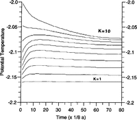
All experiments start from an ocean at rest. To assess the spin up of a modelled ocean circulation, We use the evolution of level mean temperatures during the integration to monitor the approach of stationarity (Fig. 2). Depending on the configuration, the model reaches a steady state after 20-50 years of integration.

fig.2

Run A, spin-up time. The figure displays level averaged temperatures vs integration time. While the uppermost layer (k = 1) adjusts very fast to the temperature at the ice-shelf base, thermohaline circulation needs decades to ventilate the deeper parts of the cavity.

Results

We first present the main circulation features for the sub ice- shelf cavity by means of vertically and zonally integrated mass-transport stream functions. Then, we investigate the interaction between circulation and thermohaline forcing. Finally, we compare results for open and closed northern boundaries.

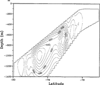
The mean meridional circulation in the sub-ice-shelf cavity is represented by the stream function for the zonally integrated mass transport shown in Figure 3a for experiment B. A northward transport near the ice-shelf base leads to strong sinking near the northern edge of the domain. Up-welling of the southward return flow occurs somewhat uniformly south of 76° S. The pattern resembles the results of Reference Hellmer and OlbersHellmer and Gibers (1991) and reflects the basic ice-pump mechanism. Compared to their results, the total transport of 0.3 Sv (1 Sv = 106m³ s ^-1) is relatively small. The circulation cell, as in Figure 3a, also prevails in experiment A (not shown); however, with even smaller transports. With the more realistic topography of case C, the circulation is somewhat modified (Fig. 3b) with down-welling south of 78° S as well as near the transition from an inclined to a flat ice shelf base further north. There is almost no meridional overturning north of 76° S, which is a rather quiet region in this experiment.

fig. 3

Stream function of the zonally integrated mass transport for experiments (a) B, and (b) C. Contour interval (a) 0.02 Sv (1Sv = 10⁶ m³ .s^-1), and (b) 0.01 Sv.

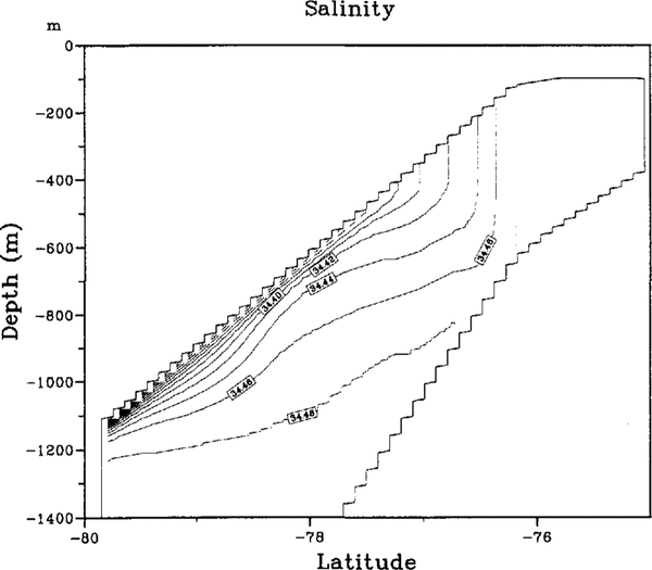
While ascending along the ice-shelf base, the water becomes super cooled with respect to the local pressure freezing point and releases ice crystals. The latent-heat release and the extraction of fresh water make the water warmer and denser. Convective mixing removes unstable density stratification arising from ice formation, resulting in a thicker homogeneous layer beneath the ice shelf. The structure of the mixed layer can be inferred from the salinity section for case C (Fig. 4) along the western boundary. Eventually, the whole water column becomes well mixed in an area of extensive ice formation north of around 77° S in this case.

fig. 4

Salinity section along the western boundary in experiment C. Contour interval is 0.02 psu (practical salinity units).

The stream function for the vertically integrated transport indicates the prevailing horizontal circulation. The northward transport in case B (Fig. 5a) is confined to the western boundary but it extends all the way through the basin. The southward return flow forms a tight recirculation near the northern edge, where the water depth gradient is small. The recirculation broadens where the ice draft increases towards the south. The slow southerly flow brings heat as a potential source of sustained melting to the grounding line. The more complicated water-column thickness gradient in case C results in a different transport pattern (Fig. 5b). A somewhat intense circulation of 2.7 Sv is centered around 78° S, where the water-depth gradient changes sign (Fig. 1a). There is no indication of a western intensification of the circulation cell. Both, the rather large amplitude and the lack of pronounced boundary currents can be explained by the reversal in sign of the background vorticity gradient, βtot = β - (f / aH)H / ∂Φ, with β = a ^-1 ∂f /∂Φ. The transports are proportional to the forcing divided by βtot in the large-scale limit. Small βtot makes the model very sensitive to changes in the forcing. As on an f plane, there is no asymmetry between eastern and western boundaries.

fig. 5

Stream function of the vertically integrated mass transport P. (a) Run B: contour interval 0.18 Sv; (b) run C: contour interval 0.20 Sv.

The buoyancy fluxes associated with melting and freezing are the only forcings for the oceanic flow in our model. The fluxes shown in Figure 6b for cases Band C are intimately coupled with the circulation itself. Generally, melting is highest where warm water meets the ice-shelf base first. This happens in the southeastern corner of the model domain. While the diluted water moves west at constant depth, melting rates become smaller until the heat potential is exhausted. Water temperatures next to the ice-shelf base now have approached Tice. During the subsequent rise with the northward current along the western boundary, the water becomes increasingly super cooled and able to release ice crystals most efficiently close to the onset of the flat part of the ice shelf. Table 1 displays the extreme values of melting and freezing for all experiments. It is obvious that ΔH_ice determines the potential for melting and freezing, and thus the magnitudes of mass exchange through the ice-shelf-ocean boundary. Comparing the two results in Figure 6, it seems that the mean circulation guides the distribution of melting and freezing areas. When a balance between horizontal advection of heat and surface heat flux is assumed for the uppermost level, the surface fresh-water flux is proportional to the velocity and the horizontal temperature gradient. Largest fluxes occur where the velocities are large and/or the temperature changes rapidly, the latter imposed by the meridional changes in ice draft. In case C, the strong currents near both the eastern and western boundaries, and their interior extensions, are locations of large fresh-water fluxes. Also, the transition from a steeply inclined to a flat ice-shelf base at 76° S stands out as an area of freezing.

fig. 6

Basal melting rates derived from model runs (a) B, and (b) C. Melting is quoted negative while basal accumul-ation appears positive. In general, strongest melting occurs in the southeastern comer of the model domain. The diluted plume propagates west, while melting rates decrease. When meeting the western boundary, a northward boundary current is initiated to transport the water, now being coldest, to more shallow ice-Shelf drafts. While rising at the ice-shelf base, the water becomes supercooled. Ice formation is soon initiated and results in maximum rates before the flat part of the ice shelf is reached at 76° S.

This is also a region of very large mixed layer depths. In case B, strong currents are confined to the western boundary and this is where the largest f1uxes occur in this case. The transition at 76° S has the same effect as in case C.

To discuss the effect of an open boundary on the internal circulation, run B seems appropriate. Because it offers the highest water column (1300m) towards the open ocean, interconnections should be most likely. The stream function for the zonally integrated transport is shown in Figure 7, which should be compared with Figure 3a. Only a small fraction of the total transport exits from the cavity and returns as a deep inflow from the open ocean. This fraction increases slightly when the frictional fluxes of momentum across the northern boundary are increased. The deep mixing due to freezing near the ice-shelf edge presents an effective barrier for the exchange with the open ocean. Since the inflow of water from the open ocean is so small, only very minor effects of the open-boundary condition are observed in the surface fresh-water f1uxes and the vertically integrated f1ow.

fig. 7

Stream function of the zonally integrated mass transport for experiment B with open-boundary conditions. Compare Figure 3a. Contour interval 0.02 Sv.

In case C, with a more realistic ice-shelf and bottom topography, the isolation of the ice-shelf cavity from the open ocean is even more pronounced. Figure 3b has already shown that in this case the circulation is mostly confined to the part with sloping ice-shelf base and bottom, and does not extend close to the northern boundary. As the difference in meridional transport (Fig. 8) proves, this remains true when the open-boundary condition is installed.

fig. 8

Difference between the zonally integrated mass transports of experiment C with open- and closed-boundary conditions. Contour interval 0.001 Sv.

Discussion and conclusions

We have presented first results from a model of the three dimensional flow beneath an ice shelf and the interaction between ocean circulation and the ice shelf. We have confined the present experiments to idealized configurations, in order to simplify the interpretation of the results. In spite of the idealized configuration, we think that some preliminary conclusions can be drawn for the actual interaction of ocean and ice shelf in Antarctica. Our results show that the ice-pump mechanism due to the pressure-dependence of the freezing point of sea water is able to explain phenomena of ice ocean interaction presently observed beneath the Ronne Ice Shelf. Modelled rates of basal melting close to the grounding line and of a subsequent accumulation of ice further north are consistent with observations and results of ice-shelf modelling (Reference DetermannDetermann, 1991; Reference Jenkins and DoakeJenkins and Doake, 1991). While the steepness of the ice-shelf base determines the potential for melting and freezing, the water-depth distribution controls the strength and direction of ocean currents initiated by ice-ocean interactions and the sites where melting and freezing occurs.

From a comparison of model experiments with open and closed boundaries towards the open ocean, we tentativcly conclude that the internal circulation of the sub-ice-shelf cavity is almost unaffected by the hydrography outside the ice-shelf front. A scenario allowing relatively warm Circumpolar Deep Water (CDW) to flush the sub-ice-shelf cavity, causing dramatic basal melting and favoring ice-shelf disintegration, is not supported by the present results. Instead, we assume that the ice-shelf water observed off several ice shelves in Antarctica originates from the near-frontal zone that IS accessible to tidal currents.

Much further modelling and observational work IS needed to confirm these findings. Currently, we are in the process of exploring carefully the full sensitivity of the model to open-boundary conditions. Also, experiments, including an open ocean north of the ice-shelf front are under way. We plan to employ our circulation model for a more realistic bottom and ice-shelf topography.

Acknowledgement

This is contribution No. 688 of the Alfred- Wegener- Institut für Polar- und Meeresforschung.