2.1. Model for neoclassical tearing mode

In this study, a set of reduced MHD equations, including bootstrap current and driven current terms (Yu et al. Reference Yu, Günter, Lackner, Gude and Maraschek2000; Liu et al. Reference Liu, Wang, Wei and Wang2022b ), in cylindrical coordinates $(r, \theta , z)$ is applied to numerically simulate the nonlinear evolution of NTMs under an RMS configuration. The set of equations includes the evolution equations for the magnetic flux, vorticity field and plasma pressure, as follows:

(2.1) \begin{align} \frac {\partial \psi }{\partial t} &= [\psi , \phi ] - \partial _z \phi - S_A^{-1}(j - j_b - j_d) + E_{z0},\\[-10pt]\nonumber \end{align}

(2.2) \begin{align} \frac {\partial u}{\partial t} &= [u, \phi ] + [j, \psi ] + \partial _z j + R_e^{-1}\boldsymbol{\nabla} _\perp ^2 u,\\[-10pt]\nonumber \end{align}

(2.3) \begin{align} \frac {\partial p}{\partial t} &= [p, \phi ] + \chi _\parallel \boldsymbol{\nabla} _\parallel ^2 p + \chi _\perp \boldsymbol{\nabla} _\perp ^2 p + S_0, \end{align}

where $\phi$ represent the streaming function; $j = - \boldsymbol{\nabla} _{\perp }^2 \psi$ and $u = \boldsymbol{\nabla} _{\perp }^2 \phi$ denote the plasma current density and vorticity along the axial direction, respectively; $j_b = f_b f(r)({\sqrt {\epsilon }}/{B_{\theta }})({\partial p}/{\partial r})$ is the bootstrap current density with $f(r)$ a function of minor radius $r$ which becomes zero as $r$ approaches the edge. The scalar parameter $f_b$ is introduced to control the global bootstrap-current fraction in the simulations and is defined as $f_b = \int _{0}^{a} j_{b0} r{\rm d}r / \int _{0}^{a} j_{z0} r{\rm d}r$ , $\epsilon = r/R_0$ is the local inverse aspect-ratio and $B_\theta$ is the poloidal magnetic field, with $R_0$ being the major radius of the tokamak. Similar to the other two current terms in (2.1), the electron cyclotron (EC) driven current density $j_d$ also undergoes nonlinear evolution along the magnetic field lines. Its evolution is described by a set of equations, which will be introduced in the next subsection. The radial coordinate $r$ is normalised by the plasma minor radius $a$ . Time $t$ and velocity $V$ are measured in units of Alfvén time $\tau _A = \sqrt {\mu _0 \rho } a / B_0$ and Alfvén velocity $V_A = B_0 / \sqrt {\mu _0 \rho }$ , respectively. Here, $S_A = \tau _\eta / \tau _A$ and $R = \tau _v / \tau _A$ are the magnetic Reynolds number and Reynolds number, respectively, where $\tau _\eta = a^2 \mu _0 / \eta$ and $\tau _v = a^2 / v$ are resistive diffusion time and viscosity diffusion time, respectively. Additionally, $\chi _\parallel$ and $\chi _\perp$ denote the parallel and perpendicular transport coefficients, respectively, which are normalised to $a^2 / \tau _A$ . The source terms $E_{z0} = S^{-1}_A (j_0 - j_{b0})$ and $S_0 = - \chi _\perp \boldsymbol{\nabla} _\perp ^2 p_0$ in (2.1) and (2.3) are chosen to balance the diffusions of initial profile of Ohm current and pressure, respectively. The Poission bracket is defined as $[f, g] = \hat {z} \boldsymbol{\cdot }\boldsymbol{\nabla }f \times \boldsymbol{\nabla }g$ .

Each variable $f(r, \theta , z, t)$ in (2.1)–(2.3) can be expressed as the sum of a time-independent equilibrium component $f_0$ and a time-dependent perturbation component $\tilde f$ , i.e. $f = f_0 + \tilde {f}(r, \theta , z, t)$ . By imposing periodic boundary conditions in the poloidal and axial directions, the perturbation fields can be Fourier-transformed and represented as

(2.4) \begin{align} \tilde {f}(r, \theta , z, t) = \frac {1}{2} \sum _{m,n} \tilde {f}_{m,n}(r, t) \exp (\mathrm{i} m \theta - \mathrm{i} n z / R_0) + \mathrm{c.c}. \end{align}

For a given initial condition, (2.1)–(2.3) can be solved using the initial-value code: MD Code. Time advancement in the numerical simulations is performed with a two-step predictor-corrector method. In the spatial coordinates, a finite difference method is applied in the radial direction, while a spectral method is employed in the poloidal and toroidal directions. The radial boundary condition is assumed to be a perfectly conducting wall.

2.2. Model for electron cyclotron resonance heating

When the CCE is included, the electron temperature perturbation induced by electron cyclotron resonance heating (ECRH) must be taken into account. It is assumed that, once ECRH is applied, a heating source is generated inside the magnetic island, and the resulting electron temperature perturbation can propagate both along and across the magnetic field lines. The evolution equation for the electron temperature perturbation can then be written as (Liu et al. Reference Liu, Wang, Wei, Wang and Reiman2024)

(2.5) \begin{align} \frac {\partial T_e}{\partial t} = \boldsymbol{\nabla }\boldsymbol{\cdot }(\chi _{f\parallel } \boldsymbol{\nabla} _\parallel T_e) + \boldsymbol{\nabla }\boldsymbol{\cdot }(\chi _{f\perp } \boldsymbol{\nabla} _\perp T_e) + \nu _f(T_h - T_e), \end{align}

where $T_e$ represent the perturbed electron temperature caused by ECRH. Here, $\chi _{f\parallel }$ and $\chi _{f\perp }$ denote the parallel and perpendicular thermal transport coefficients of electron temperature, respectively, which are normalised to $a^2 / \tau _A$ . Furthermore, $1 / \nu _f$ is the slowing-down time of the fast electrons; $T_h$ is the heating source term adopted here as Gaussian distributions in both radial direction and helical angle direction as follows:

(2.6) \begin{align} T_h = T_{h0}(w_i) \exp \left ( w_0^2 \frac {T_e}{T_{e0}} \right ) \times \exp \left \{ -4 \left [ \left ( \frac {r - r_{h0}}{\Delta r_h} \right )^2 + \left ( \frac {\xi - \xi _{h0}}{\Delta \xi _h} \right )^2 \right ] \right \}, \end{align}

where $T_{h0}$ is the magnitude of the source, in proportion to the input power of EC waves. Studies have shown that the heating efficiency is related to the magnetic island width $w_i$ . In this work, $T_{h0}$ is simplified to be linearly proportional to the magnetic island width. The parameter $w_0 = v_0 / v_{T0}$ is used to characterise the strength of the current deposition, with $v_0$ being the electron speed at the location in velocity space of greatest power deposition and $v_{T0}$ being the equilibrium electron thermal velocity. The value of $w_0$ depends on the launch position and angle of the EC wave. For efficient ECCD, $w_0^2 = 10$ is typically adopted (Reiman & Fisch Reference Reiman and Fisch2018) and temperature perturbations as high as $20\,\%$ have been measured in islands in RF stabilisation experiments (Westerhof, Lazaros & Farshi Reference Westerhof2007). Here, $T_{e0}$ denotes the electron temperature near the O-point of the magnetic island without heating; $r_{h0}$ and $\xi _{h0}$ represent the central positions of the deposition region in the radial and helical directions, respectively; while $\Delta r_h$ and $\Delta \xi _h$ represent the deposition widths in the radial and helical directions, respectively.

2.3. Model for electron cyclotron current drive

To incorporate the effect of ECCD into the set of equations, the Fisch–Boozer effect is considered (Fisch & Boozer Reference Fisch and Boozer1980), as it accurately reflects the non-local character of the EC-driven current. In this study, a closure relation is adopted, in which the driven current density is subtracted from the total current density in Ohm’s law, to represent the EC-driven current density appearing in the modified Ohm’s law of the simplified MHD equations. Electron cyclotron waves (ECWs) induce a perturbation in velocity space near the parallel resonant velocity, which can be described as a bump formed by perpendicular fast electrons and a hole formed by perpendicular slow electrons. This perturbation can be convected along magnetic field lines at the parallel resonant electron velocity from the driven current deposition region outward. Since the collision frequency is directly related to the particle velocity, the hole at low velocities is filled more quickly than the bump at high velocities is flattened. This asymmetry directly results in a net current density. The nonlinear evolution of the driven current density can be expressed as (Westerhof & Pratt Reference Westerhof and Pratt2014; Liu et al. Reference Liu, Wang, Wang and Wei2018)

(2.7) \begin{align} \frac {\partial j_{d1}}{\partial t} &= - S_j - \nu _1 j_{d1} + V_{pres} \boldsymbol{\nabla} _\parallel j_{d1},\\[-10pt]\nonumber \end{align}

(2.8) \begin{align} \frac {\partial j_{d2}}{\partial t} &= S_j - \nu _2 j_{d2} + V_{pres} \boldsymbol{\nabla} _\parallel j_{d2},\\[-10pt]\nonumber \end{align}

(2.9) \begin{align} j_d &= j_{d1} + j_{d2}, \end{align}

where $j_{d1}$ and $j_{d2}$ represent the perturbed current density driven by an EC wave through the velocity space hole filling in and the bulge decaying, respectively. Additionally, $j_d$ is the net EC-driven current density and it can be expressed as the sum of the two aforementioned components; $\nu _1$ and $\nu _2$ denote the collision frequencies during the velocity space hole filling in and the bulge decaying, respectively, normalised to the Alfvén frequency; $V_{pres}$ represents the velocity of parallel resonant electrons and is normalised to the Alfvén velocity. It is noteworthy that in (2.7) and (2.8), the signs of the driven current source term $S_j$ are opposite, ensuring the global balance of the driven current source. Moreover, the spatial distribution of $S_j$ can be assumed to follow a Gaussian profile in both the radial and helical angular directions, and is correlated with the electron temperature perturbation:

(2.10) \begin{align} S_j = S_{j0} \exp \left ( w_{rf}^2 \frac {T_e}{T_{e0}} \right ) \times \exp \left \{ -4 \left [ \left ( \frac {r - r_{h0}}{\Delta r_h} \right )^2 + \left ( \frac {\xi - \xi _{h0}}{\Delta \xi _h} \right )^2 \right ] \right \}, \end{align}

where $S_{j0}$ is the magnitude of the source and $w_{rf}$ corresponds to the resonant velocity producing the maximum current. In this study, to achieve efficient current drive, it is assumed that $w_0 = w_{rf}$ . The position parameters share the same physical meaning as those used in the electron temperature distribution.

3.1. Parameter settings

In RMS configurations with a moderate $\Delta r_s$ (the separation between the two $q = 3$ rational surface), the nonlinear evolution of the classical DTM can exhibit an explosive burst of kinetic energy (Liu et al. Reference Liu, Wang, Wang and Wei2018; Ishii et al. Reference Ishii, Azumi, Kurita and Tuda2000, Reference Ishii, Azumi and Kishimoto2002; Wang et al. Reference Wang, Wang, Dong, Lei, Long, Mou and Qu2007). The introduction of bootstrap current further destabilises islands at the outer rational surface, markedly enhancing the subsequent explosive reconnection events. Studies have shown that once the bootstrap current fraction reaches a sufficiently high level, such explosive bursts may occur even for relatively large $\Delta r_s$ (Liu et al. Reference Liu, Wang, Wang and Wei2018).

Figure 1.

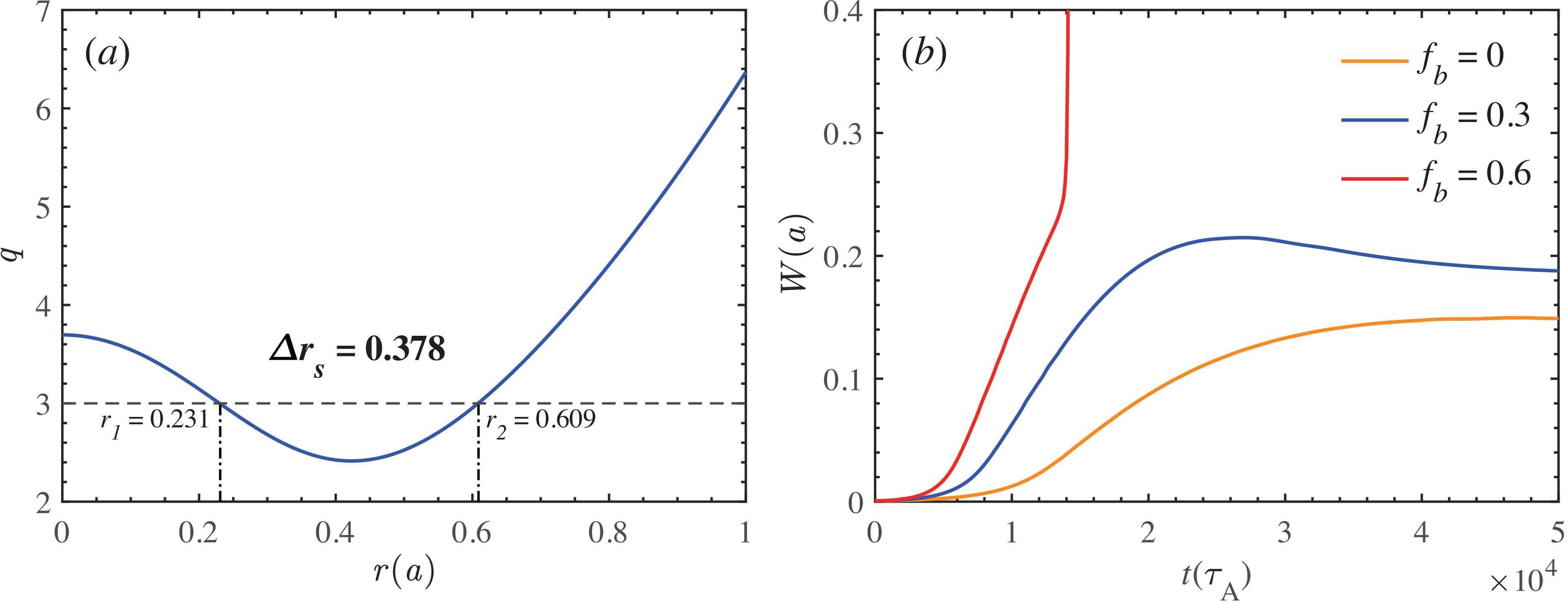
(a) An RMS safety factor profile characterised by a large separation between q = 3 rational surfaces. (b) Temporal evolutions of the magnetic island width in the outer rational surface for different bootstrap current fractions.

Figure 1. Long description

The image contains two line graphs. Panel A shows a line graph of the RMS safety factor profile characterized by a large separation between q = 3 rational surfaces. The horizontal axis is labeled r(a) and ranges from 0 to 1. The vertical axis is labeled q and ranges from 2 to 7. The graph highlights two specific points, r1 at 0.231 and r2 at 0.609, with a separation of 0.378. Panel B displays the temporal evolutions of the magnetic island width in the outer rational surface for different bootstrap current fractions. The horizontal axis is labeled t(τA) and ranges from 0 to 5 times 10^4. The vertical axis is labeled W(a) and ranges from 0 to 0.4. Three lines represent different bootstrap current fractions: fb = 0 (orange), fb = 0.3 (blue), and fb = 0.6 (red). The red line shows the steepest increase, followed by the blue line, and then the orange line.

To investigate the control of such explosive bursts, a baseline case exhibiting this phenomenon must first be established. Figure 1(a) illustrates the safety factor $q$ profile employed in this study, characterised by a large rational surface separation $\Delta r_s$ . In the JT-60U device, explosive disruptions are frequently observed and often linked to MHD activities at the $q = 3$ rational surface (Takeji et al. Reference Takeji2002). Therefore, all cases presented in this work focus on magnetic islands at the $q = 3$ rational surfaces. As shown in figure 1(b), the nonlinear evolution of outer magnetic islands is displayed by varying the bootstrap current fraction $f_b$ . The magnetic island growth rate is found to increase with $f_b$ . When $f_b = 0.3$ , the saturated width of the NTM island significantly exceeds that of the classical case with $f_b = 0$ . When $f_b$ reaches $0.6$ , an explosive burst occurs, during which the outer rational surface island rapidly grows to a large amplitude. This phenomenon is considered to be closely related to the disruption events observed during advanced tokamak discharges.

In this work, the initial pressure profile is chosen in the form of $p_0 (r) = (1 - r^2)^6$ . A rigid rotation profile with no frequency difference in the radial direction is applied in the cases with rotary magnetic islands. The rotation frequency is set as $\omega _0 = 0.01$ . Additionally, other typical parameters are specified as follows: $\epsilon _0 = a/R_0 = 0.25$ , $S_A^{-1} = 10^{-6}$ , $R^{-1} = 10^{-6}$ , $\chi _\parallel = 10$ and $\chi _\perp = 10^{-6}$ . Unless stated otherwise, the typical parameters associated with the ECRH and ECCD are as follows: $\chi _{f\parallel } = 10$ , $\chi _{f\perp } = 10^{-7}$ , $\nu _f = 2 \times 10^{-3}$ , $w_0^2 = w_{rf}^2 = 10$ , $\nu _1 = 2.5 \times 10^{-3}$ , $\nu _2 = 0.5 \times 10^{-3}$ , $V_{pres} = 2$ , $r_{h0} = r_{d0} = 0.609$ , $\xi _{h0} = \xi _{d0} = \pi$ , $\Delta r_h = \Delta r_d = 0.2$ and $\Delta \xi _h = \Delta \xi _d = 0.8 \times 2\pi$ .

According to the theory of the CCE, under a certain level of ECCD injection power, the system may exhibit two solutions, referred to as the ‘upper-branch’ and ‘lower-branch’ solutions (Reiman & Fisch Reference Reiman and Fisch2018; Liu et al. Reference Liu, Wang, Wei, Wang and Reiman2024). The upper-branch solution corresponds to stronger temperature perturbations and a more pronounced CCE. However, it is physically unstable and can only be realised once the excitation threshold is reached. In the physical model employed in this study, exceeding this threshold leads to unbounded temperature growth, though the inclusion of additional physical effects, such as wave dissipation, can result in a third solution (Rodríguez et al. Reference Rodríguez, Reiman and Fisch2019). The present study considers only the lower-branch solution within the threshold range.

3.2. Stabilisation of classical tearing mode in reversed magnetic shear $(f_b = 0)$

To establish a baseline for assessing the enhancement of CCE on ECCD, we first examine its stabilising capability in classical cases. Based on previous findings, the dominant magnetic island during the nonlinear evolution is located at the outer rational surface (Janvier et al. Reference Janvier, Kishimoto and Li2011). Therefore, a Gaussian-distributed ECCD current is injected at the outer rational surface $r_s = 0.609$ of the initial $q$ profile. The ECCD is turned on at $t = 5.5 \times 10^4$ , corresponding to the post-saturation phase of the mode, and different strengths of the driven current are introduced. This allows the saturated magnetic island to be controlled to different degrees.

Figure 2.

Temporal evolutions of the magnetic island width in the outer rational surface for (a) different magnitudes of EC-driven current, (b)–(d) ECCD with different strengths of the CCE without plasma rotation. The ECCD is turned on at $t = 5.5 \times 10^4$ .

In the absence of plasma rotation, figure 2 presents the temporal evolution of the magnetic island width under different driven current magnitudes. Figure 2(a) illustrates the control effectiveness of conventional ECCD on the mode. Here, the amplitude $S_{j0}$ in the current source distribution equation is used to represent the relative strength of the driven current. It can be observed that conventional ECCD is capable of suppressing the magnetic island. As the driven current strength increases, the saturated island width gradually decreases. When the power becomes sufficiently high, the magnetic island can be completely suppressed. Building upon the three controlling conditions described previously, the CCE is incorporated, as shown in figure 2(b–d). Here, the temperature-dependent term in the heating and driven current sources is quantified by the temperature differential parameter $U_0 = w_s^2 ({\widetilde {T}_O}/{T_S})$ , which is used as an indicator of the strength of the CCE. Within the magnetic island, the electron temperature profile can be considered flattened. Therefore, the electron temperature near the separatrix $T_S$ is assumed to be equal to that near the O-point, i.e. $T_S = T_O$ . The quantity $\widetilde {T}_O$ represents the temperature perturbation inside the island induced by the ECRH. It can be observed that the CCE significantly enhances the ECCD control capability: the saturated island width is markedly reduced and the rate of island shrinkage is substantially accelerated. Furthermore, as the CCE becomes stronger, the enhancement of the ECCD control performance becomes more pronounced.

3.3. Stabilisation of neoclassical tearing mode with moderate bootstrap current $(f_b = 0.3)$

Based on the conclusions regarding classical TM without bootstrap current in the previous section, the bootstrap current effect is further introduced. The inclusion of the bootstrap current complicates the physical processes of TM dynamics, leading to magnetic islands that grow faster and reach larger saturated widths. Consequently, NTMs are more challenging to control with conventional ECCD than their classical counterparts. Larger islands require stronger input power of ECW, and the control effectiveness of a given input power decreases. Previous numerical simulations have supported this concept (Wang et al. Reference Wang, Yu, Zhang, Zhu, Wang and Wu2017; Liu et al. Reference Liu, Wang, Wang and Wei2018; Liu et al. Reference Liu, Wang, Wei and Wang2022b ). However, experimental observations reveal a contrasting phenomenon: the control efficiency of ECCD on magnetic islands is higher than predicted by numerical simulations and this effect is particularly pronounced for large islands. The CCE provides a physical explanation for this behaviour by introducing two mechanisms that collectively enhance ECCD control efficiency. First, thermal insulation within the island allows localised temperature accumulation, creating a positive feedback loop via the CCE. Second, the CCE preferentially focuses driven current deposition towards the island O-point. These insights suggest that the previously advocated strategy of ‘early ECCD application’ may not always be optimal for stabilising NTM islands.

To quantify the efficiency of ECCD in controlling magnetic islands, this section introduces the concept of ‘the total stabilising time’, defined as the time interval from ECCD initiation to complete island suppression. This metric is used to investigate whether applying ECCD at a later stage for larger islands can achieve more effective control under certain parameter conditions.

Figure 3.

Temporal evolutions of island width under control of ECCD at different island widths with (a) weak, (b) moderate and (c) strong CCE.

Figure 3. Long description

Three line graphs depict the temporal evolutions of island width under different control conditions. Panel A: The line graph shows the evolution of island width with weak CCE. The x-axis represents time in units of t(τA) × 10^4, ranging from 0 to 5. The y-axis represents the island width W(a), ranging from 0 to 0.25. Three lines in different colors (green, blue, and red) represent different scenarios with specific island widths and time intervals labeled. Panel B: The line graph shows the evolution of island width with moderate CCE. The x-axis and y-axis are the same as in Panel A. Three lines in different colors (green, blue, and red) represent different scenarios with specific island widths and time intervals labeled. Panel C: The line graph shows the evolution of island width with strong CCE. The x-axis and y-axis are the same as in Panels A and B. Three lines in different colors (green, blue, and red) represent different scenarios with specific island widths and time intervals labeled.

For a bootstrap current fraction of $f_b = 0.3$ , the evolution of the magnetic island at the outer rational surface is shown by the blue line in figure 1(b). Prior to the island reaching its maximum width, ECCD incorporating the CCE is applied at three different time points to ensure that ECCD acts on islands of different sizes. The input power of the driven current is kept constant and the resulting control effects on the magnetic island are presented in figure 3. As shown in figure 3, the blue curve represents the case where ECCD is turned on at $t_1 = 1.6 \times 10^4$ , corresponding to a relatively small island width; the red curve corresponds to $t_2 = 1.8 \times 10^4$ , when the magnetic island has grown to a moderate size; while the green curve indicates the latest ECCD activation time $t_3 = 2.4 \times 10^4$ , at which the island reaches the largest width among the three cases. The grey dashed curves in figure 3(a) are included as reference cases in which the same ECCD power and turn-on times are used, but the condensation effect is switched off. When the CCE is relatively weak, as shown in figure 3(a), the magnetic island width primarily determines the total stabilising time and smaller islands require less time to be controlled, i.e. $\Delta t_1 \lt \Delta t_2 \lt \Delta t_3$ . As the temperature perturbation increases, the strength of the CCE also rises, as illustrated in figure 3(b). In this case, the control of larger islands is enhanced more significantly, resulting in a greater reduction in the total stabilising time for large islands compared with smaller ones, i.e. $\Delta t_5 \lt \Delta t_4$ . The enhancement of ECCD by the CCE exhibits a nonlinear dependence on the input power. Near the threshold, higher input power can induce a very strong CCE. When the input power approaches the threshold, applying ECCD to larger islands can yield a shorter total stabilising time than that to smaller islands, i.e. $\Delta t_9 \lt \Delta t_8 \lt \Delta t_7$ .

Figure 4.

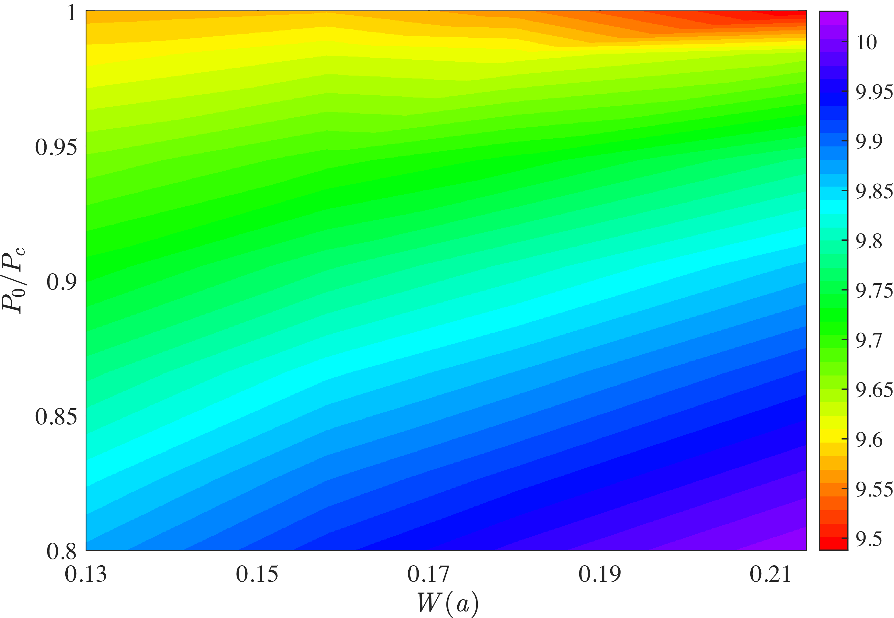
Dependence of the stabilisation time on the magnetic island width and the normaliesd strength of the CCE.

Figure 4 illustrates the dependence of the stabilisation time on both the island width at the onset of ECCD with CCE and the normalised ECCD input power $(P_0 / P_c)$ , where $P_c$ is the power threshold for the fold bifurcation (Wang et al. Reference Wang, Yu, Zhang, Zhu, Wang and Wu2017). The different colours indicate the stabilisation time of the magnetic island. The data are plotted on a logarithmic scale to better illustrate the trend. In the lower part of figure 4, the colour distribution clearly transitions from the bottom right to the upper left, which indicates that suppressing larger islands requires higher input power. However, this trend is reversed at the upper right. As the strength of the CCE gradually approaches its threshold value, the regions of shortest stabilisation time shift towards larger island widths. When $P_0 / P_c$ approaches unity, the nonlinear positive feedback induced by CCE enhances the localisation of the driven current around the island O-point, leading to faster stabilisation for larger islands. This phenomenon, where large magnetic islands become more controllable, occurs only near the threshold (within this work) and becomes more pronounced as this threshold is approached.

Based on the above-mentioned results, a more effective strategy for controlling NTMs can be developed. Under the influence of the CCE, appropriately delaying the application of ECCD may lead to higher control efficiency. Previous studies have also suggested that applying ECCD after the magnetic island has grown sufficiently large and become locked can be a more favourable approach under certain conditions. However, excessive delay in ECCD activation, which allows the NTM island to grow freely, may increase the risk of triggering explosive burst events. In the next section, the onset of explosive bursts will be intentionally induced to investigate the control performance of ECCD in the presence of the CCE.

3.4. Suppression of the explosive burst with strong bootstrap current $(f_b = 0.6)$

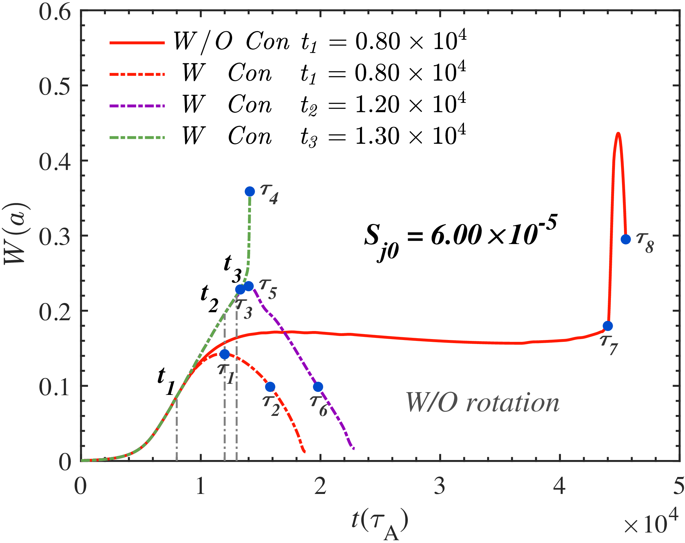
By further incorporating the CCE, the control capability against the explosive burst event is significantly enhanced. As illustrated by the red dash-dotted line in figure 6, with the same EC input power, the inclusion of CCE allows complete stabilisation of the magnetic island that could otherwise trigger a disruption due to the delayed ECCD activation. This improvement in performance thereby allows for a later initiation of ECCD. As shown by the purple dash-dotted line, even when the ECCD is initiated at $t_2 = 1.2 \times 10^4$ , the island remains fully stabilised, while a further delay to $t_3 = 1.3 \times 10^4$ leads to the onset of the explosive burst event. Under the present simulation parameters, the CCE extends the permissible ECCD response time by approximately $70\,\%$ without requiring additional control. This illustrates that the condensation mechanism not only improves current drive efficiency, but also provides crucial extra margin for disruption avoidance in future tokamak operation scenarios, such as those in ITER.

Figure 7.

Contours of the magnetic island at eight moments without plasma rotation shown in figure 6: (a) $\tau _1 = 1.20 \times 10^4$ ; (b) $\tau _2 = 1.58 \times 10^4$ ; (c) $\tau _3 = 1.33 \times 10^4$ ; (d) $\tau _4 = 1.41 \times 10^4$ ; (e) $\tau _5 = 1.40 \times 10^4$ ; (f) $\tau _6 = 1.98 \times 10^4$ ; (g) $\tau _7 = 4.40 \times 10^4$ ; (h) $\tau _8 = 4.55 \times 10^4$ .

Figure 7. Long description

Eight contour plots show the evolution of magnetic islands at different moments without plasma rotation. Each plot is labeled with a specific time (τ) value. Panel A: The contour plot at τ1 = 1.20 x 10^4 shows a central region with concentric contours, indicating the magnetic island structure. Panel B: The contour plot at τ2 = 1.58 x 10^4 displays a similar structure with slightly altered contours. Panel C: The contour plot at τ3 = 1.33 x 10^4 shows a more complex pattern with additional contours. Panel D: The contour plot at τ4 = 1.41 x 10^4 exhibits further changes in the contour pattern. Panel E: The contour plot at τ5 = 1.40 x 10^4 shows a more intricate structure with multiple contours. Panel F: The contour plot at τ6 = 1.98 x 10^4 displays a different arrangement of contours. Panel G: The contour plot at τ7 = 4.40 x 10^4 shows a complex pattern with numerous contours. Panel H: The contour plot at τ8 = 4.55 x 10^4 exhibits a highly detailed structure with many contours. Each plot has axes labeled R - R0 and Z, with units in centimeters.

Figure 8.

Contours of the EC current density at eight moments without plasma rotation shown in figure 6: (a) $\tau _1 = 1.20 \times 10^4$ ; (b) $\tau _2 = 1.58 \times 10^4$ ; (c) $\tau _3 = 1.33 \times 10^4$ ; (d) $\tau _4 = 1.41 \times 10^4$ ; (e) $\tau _5 = 1.40 \times 10^4$ ; (f) $\tau _6 = 1.98 \times 10^4$ ; (g) $\tau _7 = 4.40 \times 10^4$ ; (h) $\tau _8 = 4.55 \times 10^4$ .

Figure 9.

Contours of the stream function at eight moments without plasma rotation shown in figure 6: (a) $\tau _1 = 1.20 \times 10^4$ ; (b) $\tau _2 = 1.58 \times 10^4$ ; (c) $\tau _3 = 1.33 \times 10^4$ ; (d) $\tau _4 = 1.41 \times 10^4$ ; (e) $\tau _5 = 1.40 \times 10^4$ ; (f) $\tau _6 = 1.98 \times 10^4$ ; (g) $\tau _7 = 4.40 \times 10^4$ ; (h) $\tau _8 = 4.55 \times 10^4$ .

Figure 9. Long description

Panel A: A heat map showing the stream function contours at a moment with a value of 1.20 x 10^4. The x-axis is labeled R - R0 and ranges from -0.5 to 0.5. The y-axis is labeled Z and ranges from -0.5 to 0.5. The heat map displays a pattern of alternating red and blue regions, indicating variations in the stream function. Panel B: A heat map showing the stream function contours at a moment with a value of 1.58 x 10^4. The axes and their ranges are the same as in Panel A. The pattern of red and blue regions is similar but slightly different in distribution. Panel C: A heat map showing the stream function contours at a moment with a value of 1.33 x 10^4. The axes and their ranges are the same as in Panel A. The pattern of red and blue regions shows further evolution. Panel D: A heat map showing the stream function contours at a moment with a value of 1.41 x 10^4. The axes and their ranges are the same as in Panel A. The pattern of red and blue regions continues to evolve. Panel E: A heat map showing the stream function contours at a moment with a value of 1.40 x 10^4. The axes and their ranges are the same as in Panel A. The pattern of red and blue regions shows further changes. Panel F: A heat map showing the stream function contours at a moment with a value of 1.98 x 10^4. The axes and their ranges are the same as in Panel A. The pattern of red and blue regions continues to evolve. Panel G: A heat map showing the stream function contours at a moment with a value of 4.40 x 10^4. The axes and their ranges are the same as in Panel A. The pattern of red and blue regions shows significant changes. Panel H: A heat map showing the stream function contours at a moment with a value of 4.55 x 10^4. The axes and their ranges are the same as in Panel A. The pattern of red and blue regions shows further evolution.

Figure 5.

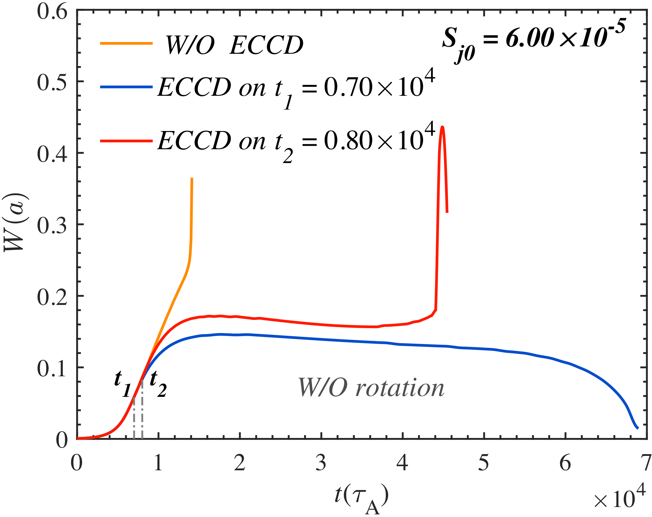
Temporal evolutions of the magnetic island width in the outer rational surface for different ECCD turn-on time without plasma rotation.

For a steady-state operation, a high bootstrap current fraction is required and an RMS configuration is often recommended. However, a high bootstrap current fraction tends to trigger explosive burst events, as illustrated by the red curve in figure 1(b), where an explosive burst occurs when the bootstrap current fraction reaches approximately $60\,\%$ under this condition. According to the conventional ECCD model, suppressing such explosive bursts can be achieved in a straightforward manner by increasing the ECCD power or advancing the injection timing. However, according to the conclusions drawn in the previous section, it is worthwhile to explore a more economical and efficient ECCD control strategy, and to investigate whether the CCE can assist in suppressing explosive bursts during the later stages of magnetic island evolution.

It is generally believed that, as long as the ECCD is applied sufficiently early, the explosive burst can be completely suppressed with a certain level of input power, as shown by the blue line in figure 5, which depicts the temporal evolution of the island width. However, if the ECCD is not activated in time, the same input power may fail to suppress the island. As indicated by the red line in figure 5, under the present parameter settings, a delay of merely 1000 Alfvén times (of the order of milliseconds) can lead to the occurrence of an explosive burst, which would be extremely critical and hazardous in practical tokamak operations.

Figure 6.

Time evolution of the magnetic island width with and without the CCE under different ECCD onset times. The ECCD input power is kept constant at $S_{j0} = 6.00 \times 10^{-5}$ and plasma rotation is not included in these simulations.

In addition, to provide a clearer visualisation of the underlying physical processes, the spatial distributions of the magnetic flux, EC-driven current and stream function at different evolution stages are shown in figures 7, 8 and 9, corresponding to the cases in figure 6. These three quantities provide complementary information on the stabilisation process. The magnetic-flux contours characterise the island topology and the nonlinear interaction between the inner and outer rational surfaces. The EC-driven current distribution indicates the degree of localisation of the stabilising current relative to the island O-point, where compensation of the bootstrap current deficit is most effective. The stream function describes the associated nonlinear flow response, which affects pressure convection, island deformation and magnetic reconnection. For the scenario where the magnetic island is completely stabilised, the times $\tau _1$ , $\tau _2$ , $\tau _5$ and $\tau _6$ are selected to represent the stages when the island reaches its maximum width and when it is suppressed to an equivalent level. In contrast, $\tau _3$ , $\tau _4$ , $\tau _7$ and $\tau _8$ correspond to the moments just before and during the onset of the explosive burst.

For the red dash-dotted and purple dash-dotted cases with CCE, figures 7(a) and 7(e) ( $\tau _1$ and $\tau _5$ ) correspond to the moments when the magnetic island attains its maximum width prior to complete suppression. It can be clearly observed that the magnetic island at $\tau _5$ is significantly larger than that at $\tau _1$ . The inner magnetic island also grows noticeably and exerts an outward compression on the outer island, resulting in a more intricate and distorted nested magnetic topology. Figures 7(b) and 7(f) ( $\tau _2$ and $\tau _6$ ) are taken when the island has been suppressed to $0.1$ . The contours show progressive restoration of nested flux surfaces as the EC current, enhanced by CCE, concentrates near the O-point and accelerates shrinkage. For the red solid (without CCE) and green dash-dotted (with CCE) cases that exhibit explosive behaviour, figures 7(c) and 7(g) ( $\tau _3$ and $\tau _7$ ) denote the states immediately before the explosive growth, where strong distortion layers appear around the separatrix. Figures 7(d) and 7(h) ( $\tau _4$ and $\tau _8$ ) show that, corresponding to the stages following the onset of the explosive burst event, the compression between the inner and outer magnetic islands becomes more pronounced. An evident island exchange phenomenon emerges, which may further evolve into magnetic topology breakup, leading to extensive magnetic stochasticity. The different topological evolution in the controllable and explosive cases indicates that the subsequent island dynamics is governed not only by the instantaneous island width, but also by the spatially localised compensation of the bootstrap current deficit. In the cases stabilised with the CCE, although the island is relatively large and the nonlinear interaction between the inner and outer rational surfaces is already appreciable, the nested flux surfaces are progressively recovered after ECCD is applied. This behaviour is attributed to the nonlinear temperature response inside the island: the CCE enhances the EC-driven current around the island O-point, where the bootstrap current deficit produced by pressure flattening is most effectively compensated. The resulting O-point current condensation reduces the tearing drive and weakens the coupling between the inner and outer islands, thereby preventing the system from entering the fast-reconnection regime. By contrast, in the explosive cases, the compression between the inner and outer islands continues to increase and the island-exchange structure becomes evident. This reflects a strong nonlinear coupling of the two $q = 3$ rational surfaces. Once the bootstrap-current deficit is not compensated sufficiently, the distorted magnetic topology, pressure flattening and reconnection flow reinforce each other, leading to rapid island expansion and the loss of nested magnetic surfaces. Therefore, the comparison in figure 7 provides direct topological evidence that the CCE suppresses the explosive burst by localising the stabilising EC-driven current at the O-point and interrupting the positive feedback between bootstrap current deficit and nonlinear island coupling.

Figure 8 presents the spatial distributions of the EC-driven current density $j_d$ at the eight characteristic time points ( $\tau _1$ – $\tau _8$ ) corresponding to those in figure 6. These plots illustrate how the localisation and intensity of the driven current evolve under different control scenarios, with and without the CCE. For the red dash-dotted and purple dash-dotted cases with CCE, the driven current exhibits a strong localisation around the O-point of the outer magnetic island. Figures 8(a) and 8(e) ( $\tau _1$ and $\tau _5$ ) show that the stronger inward shift of the outer rational surface at $\tau _5$ causes the deposition centre to move radially inward, leading to the formation of a hollow region in the EC-driven current density profile. Figures 8(b) and 8(f) ( $\tau _2$ and $\tau _6$ ) show that the deposition region becomes further narrowed with the islands decaying. It is also evident that the driven current distribution at $\tau _6$ is broader than that at $\tau _2$ . Owing to the CCE, the enhanced driven current does not vanish immediately, but instead exhibits a hysteresis-like behaviour. For the red solid (without CCE) and green dash-dotted (with CCE) cases that exhibit explosive behaviour, the asymmetry of the driven current distribution becomes significantly more pronounced. Figures 8(c) and 8(g) ( $\tau _3$ and $\tau _7$ ) show that, under the same injected EC power, the driven current at $\tau _3$ is evidently more concentrated around the O-points of the islands, further confirming the enhancement effect of CCE on ECCD efficiency. During the explosive burst, figures 8(d) and 8(h) ( $\tau _4$ and $\tau _8$ ) display that even though the driven current is deposited in the whole island area, the burst can still happen. The comparison of the driven-current distributions highlights the mechanism by which the CCE improves the effectiveness of ECCD. In the absence of the CCE, the stabilising effect is mainly determined by the externally imposed EC current source and by its geometrical overlap with the island. When the CCE is included, the local temperature perturbation inside the island produces a nonlinear enhancement of the driven current, causing the current source to be preferentially concentrated near the O-point. This localisation is crucial, since the O-point region is where the bootstrap-current deficit associated with pressure flattening is most effectively compensated. Thus, the CCE does not simply increase the driven-current amplitude; rather, it improves the spatial phase relation between the stabilising current and the magnetic island. The persistence of the enhanced current during the island-decay phase further reflects the hysteresis-like nature of the condensation process. Once the temperature perturbation and current localisation are established in a sufficiently large island, the enhanced EC-driven current remains effective even as the island begins to shrink. This delayed relaxation provides a sustained stabilising contribution to the magnetic flux evolution and accelerates the recovery of the island topology. In the explosive cases, however, the magnetic topology evolves rapidly and the driven current becomes less effectively correlated with the instantaneous O-point structure. Consequently, even when the EC-driven current spreads over a broad island region, it cannot compensate the bootstrap current deficit sufficiently rapidly to interrupt the nonlinear reconnection process. Figure 8 therefore supports the interpretation that the principal role of the CCE is to reinforce the O-point-localised current compensation and to maintain this compensation over the island decay phase.

Figure 9 presents the distributions of the stream function $\phi$ at the eight characteristic time points ( $\tau _1$ – $\tau _8$ ) corresponding to those in figure 6. These plots reveal the evolution of the perturbed velocity structure associated with magnetic island dynamics and ECCD modulation, under both the presence and absence of the CCE. Figures 9(a) and 9(e) ( $\tau _1$ and $\tau _5$ ) show that the vortices expand to cover a broader area within the magnetic island for a larger island width and the higher-order harmonics become significant. Figures 9(b) and 9(f) ( $\tau _2$ and $\tau _6$ ) show that, during the decay phase of the mode, reversed vortices appear in the vicinity of the X-point. Figures 9(c) and 9(g) ( $\tau _3$ and $\tau _7$ ) show that the vortices within the inner islands become significant due to the control of the outer island. During the explosive burs, figures 9(d) and 9(h) ( $\tau _4$ and $\tau _8$ ) display that only low-order harmonics of vortices play important roles. The stream-function structures provide further information on how the nonlinear flow response is modified during stabilisation and explosive growth. In the reduced-MHD description, the stream function is associated with the convective motion of the plasma, and therefore influences the redistribution of pressure perturbations and the deformation of the magnetic island. In the cases stabilised by CCE-enhanced ECCD, the localised compensation of the bootstrap current deficit weakens the tearing drive and the flow pattern becomes increasingly consistent with island shrinkage. The appearance of reversed vortical structures near the X-point during the decay phase suggests a reorganisation of the flow field that is unfavourable to further island expansion and is consistent with the restoration of nested magnetic surfaces. In contrast, in the explosive cases, the flow field is dominated by large-scale low-order vortical structures. Such structures indicate that the flow is no longer a secondary perturbation to the island dynamics, but participates in the nonlinear feedback between island deformation, pressure redistribution and magnetic reconnection. This large-scale convective response can enhance the compression and exchange between the inner and outer islands, thereby accelerating the loss of regular magnetic topology. The comparison in figure 9 therefore indicates that the CCE affects the explosive dynamics not only through the current profile, but also indirectly through the flow response: by reducing the tearing drive through O-point current condensation, the CCE suppresses the development of the large-scale vortical structures that accompany rapid island growth.

Taken together, figures 7, 8 and 9 clarify the physical pathway through which the CCE enhances ECCD and prevents the explosive burst. The magnetic-flux contours show whether the system evolves towards restoration of nested magnetic surfaces or towards island exchange and topology degradation. The EC-driven-current contours identify the degree to which the stabilising current is localised at the O-point, where compensation of the bootstrap current deficit is most effective. The stream-function contours reveal the nonlinear flow response associated with pressure convection, island deformation and reconnection. In the successfully stabilised cases, these three aspects are mutually consistent: the CCE concentrates the driven current near the O-point, this localised current reduces the bootstrap-current deficit and weakens the tearing drive, and the associated flow response no longer supports rapid island expansion. As a result, the island topology recovers before the nonlinear coupling between the two $q = 3$ rational surfaces develops into an explosive event. In the explosive cases, the opposite tendency is observed. The driven current is either insufficiently localised or becomes poorly correlated with the rapidly evolving O-point structure, while the inner and outer island coupling and large-scale flow response continue to strengthen. Under these conditions, the bootstrap current deficit, magnetic-topology distortion and nonlinear convection reinforce one another, leading to rapid island growth. The contour analysis therefore supports the conclusion drawn from the island-width evolution: at the same EC input power, the CCE extends the permissible ECCD response window by creating a self-reinforcing, O-point-localised stabilising current that interrupts the positive feedback responsible for explosive burst formation.

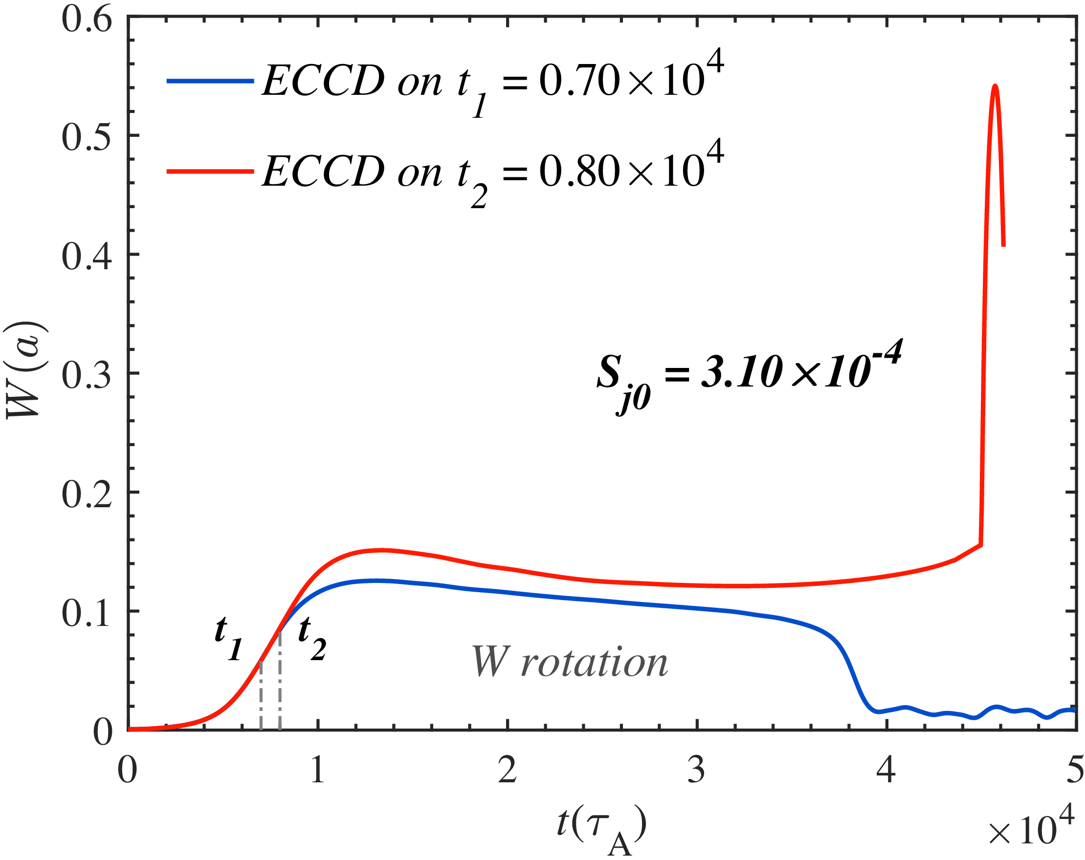
Figure 10 illustrates the time evolution of the magnetic island width under the condition of rigid plasma rotation ( $\omega _0 = 0.01$ ). In this case, a higher input power is required to achieve complete stabilisation when the ECCD is applied at the same onset time. This is because plasma rotation causes the driven current to alternately deposit near the O-point and the X-point of the magnetic island, resulting in successive stabilisation and destabilisation phases (Liu et al. Reference Liu, Wang, Wang and Wei2018). When rotation is included, to more clearly highlight the influence of the driven current, the typical control parameters are adjusted to $\Delta r_h = \Delta r_d = 0.1$ and $\Delta \xi _h = \Delta \xi _d = 0.4 \times 2 \pi$ . In the rotating cases, the island periodically moves relative to the fixed ECCD deposition region, so that the driven current alternately acts near the O-point and the X-point. A narrower deposition profile is therefore adopted to keep the EC source more localised and to avoid an excessively broad overlap with the island region, which can otherwise mix stabilising and destabilising phases. Consequently, the rotating cases are intended mainly as a qualitative test of whether the CCE can still enhance ECCD under rotation-induced phase mismatch, rather than as a strict quantitative comparison with the non-rotating cases. As shown by the red curve in figure 10, when the ECCD input power is kept constant, a delay of merely 1000 Alfvén times in the activation leads to the onset of an explosive event. Based on this, the same input power is subsequently used with the CCE to investigate its capability in suppressing the explosive burst in rotating plasmas.

Figure 10.

Temporal evolutions of the magnetic island width in the outer rational surface for different ECCD turn-on time with plasma rotation ( $\omega _0 = 0.01$ ).

Figure 11.

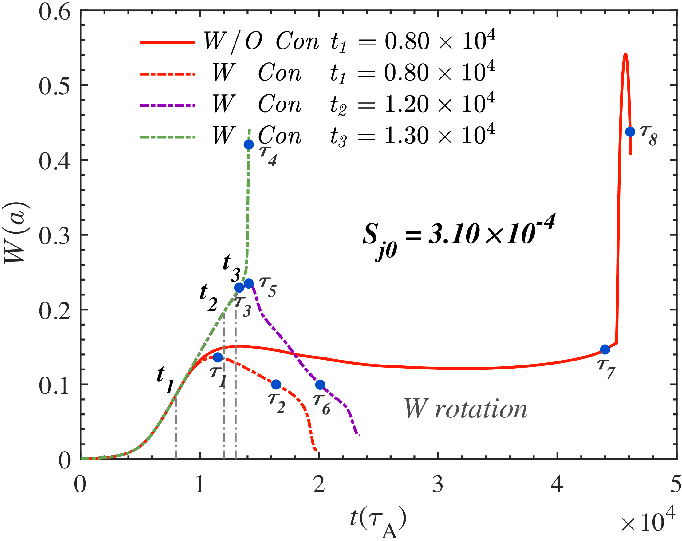
Time evolution of the magnetic island width with and without the CCE under different ECCD onset times. The ECCD input power is kept constant at $S_{j0} = 3.10 \times 10^{-4}$ and plasma rotation is included in these simulations.

Figure 11. Long description

A line graph showing the time evolution of magnetic island width with and without CCE under different ECCD onset times. The horizontal axis represents time in units of 10^4 tau_A, ranging from 0 to 5. The vertical axis represents the magnetic island width W(a), ranging from 0 to 0.6. The graph includes four data lines: a solid red line labeled ’W/O Con t1 = 0.80 x 10^4’, a dashed red line labeled ’W Con t1 = 0.80 x 10^4’, a dashed purple line labeled ’W Con t2 = 1.20 x 10^4’, and a dashed green line labeled ’W Con t3 = 1.30 x 10^4’. Key points on the graph are marked with blue dots and labeled with tau symbols (tau_1 to tau_8). The graph shows the evolution of magnetic island width over time for different ECCD onset times, with notable peaks and troughs indicating changes in width.

Similarly, the inclusion of the CCE enables complete stabilisation of the magnetic island that cannot be controlled by conventional ECCD, as indicated by the red dash-dotted curve in figure 11. Moreover, CCE effectively extends the available response time for disruption avoidance under the same ECCD input power. As shown by the purple and green dash-dotted curves in figure 11, the ECCD activation can be postponed up to the time $t_2 = 1.2 \times 10^4$ without triggering the explosive event, demonstrating the significant enhancement of control robustness provided by CCE in rotating plasmas. Also, the same eight evolution stages as those in the previous analysis are selected. Figures 12, 13 and 14 present the spatial distributions of the magnetic island, EC-driven current and stream function corresponding to the time points indicated in figure 11.

Figure 12 presents the magnetic island contours at eight characteristic time points ( $\tau _1$ – $\tau _8$ ) under the condition of rigid plasma rotation $(\omega _0 = 0.01)$ , corresponding to those in figure 11. The selection of these time points follows the same logic as in the non-rotating cases to facilitate a direct comparison of the effects introduced by plasma rotation. Compared with figure 7, plasma rotation slows down the recovery of the nested magnetic-surface structure on some level. Figures 12(a–c) and 12(e–g) ( $\tau _1$ – $\tau _3$ and $\tau _5$ – $\tau _7$ ) are similar to those in figure 7, representing the same island-evolution stages. In the absence of CCE, the outer island compression at $\tau _7$ becomes more pronounced, and the inner–outer island exchange process is more intense. In contrast, when CCE is included, the configuration at $\tau _3$ shows no significant deviation from the non-rotating case at the same evolution time. Figures 12(d) and 12(h) ( $\tau _4$ – $\tau _8$ ) correspond to the explosive burst stages, during which the magnetic-surface topology at $\tau _8$ undergoes severe deformation, exhibiting increased distortion. Overall, the inclusion of plasma rotation weakens the stability of the magnetic-surface topology, whereas the CCE retains its stabilising capability even in rotating plasmas.

Figure 12.

Contours of the magnetic island at eight moments with plasma rotation $(\omega _0 = 0.01)$ shown in figure 11: (a) $\tau _1 = 1.15 \times 10^4$ ; (b) $\tau _2 = 1.64 \times 10^4$ ; (c) $\tau _3 = 1.33 \times 10^4$ ; (d) $\tau _4 = 1.41 \times 10^4$ ; (e) $\tau _5 = 1.41 \times 10^4$ ; (f) $\tau _6 = 2.01 \times 10^4$ ; (g) $\tau _7 = 4.40 \times 10^4$ ; (h) $\tau _8 = 4.55 \times 10^4$ .

Figure 13.

Contours of the EC current density at eight moments with plasma rotation $(\omega _0 = 0.01)$ shown in figure 11: (a) $\tau _1 = 1.15 \times 10^4$ ; (b) $\tau _2 = 1.64 \times 10^4$ ; (c) $\tau _3 = 1.33 \times 10^4$ ; (d) $\tau _4 = 1.41 \times 10^4$ ; (e) $\tau _5 = 1.41 \times 10^4$ ; (f) $\tau _6 = 2.01 \times 10^4$ ; (g) $\tau _7 = 4.40 \times 10^4$ ; (h) $\tau _8 = 4.55 \times 10^4$ .

Figure 13. Long description

Panel A: A heat map showing the EC current density distribution with a circular pattern. The z-axis ranges from -0.5 to 0.5, and the R-R0 axis ranges from -0.5 to 0.5. The color scale indicates intensity, with red representing higher values and blue representing lower values. The highest intensity is observed in a circular band. Panel B: A heat map showing the EC current density distribution with a slightly more defined circular pattern compared to Panel A. The axes and color scale are the same as in Panel A. The highest intensity remains in a circular band, but it is more pronounced. Panel C: A heat map showing the EC current density distribution with a triangular pattern. The axes and color scale are the same as in previous panels. The highest intensity is observed in three distinct regions forming a triangular shape. Panel D: A heat map showing the EC current density distribution with a more complex pattern. The axes and color scale are the same as in previous panels. The highest intensity is observed in three distinct regions forming a more complex shape. Panel E: A heat map showing the EC current density distribution with a triangular pattern similar to Panel C but with more defined regions. The axes and color scale are the same as in previous panels. The highest intensity is observed in three distinct regions forming a triangular shape. Panel F: A heat map showing the EC current density distribution with a circular pattern similar to Panel B. The axes and color scale are the same as in previous panels. The highest intensity remains in a circular band. Panel G: A heat map showing the EC current density distribution with a more complex pattern. The axes and color scale are the same as in previous panels. The highest intensity is observed in a more complex shape. Panel H: A heat map showing the EC current density distribution with a pattern similar to Panel D but with more defined regions. The axes and color scale are the same as in previous panels. The highest intensity is observed in three distinct regions forming a more complex shape.

Figure 13 presents the spatial distributions of the EC-driven current density $j_d$ at the eight characteristic time points ( $\tau _1$ – $\tau _8$ ) under rigid plasma rotation $(\omega _0 = 0.01)$ , corresponding to the cases shown in figure 11. Compared with the non-rotating cases, the deposition region of the driven current becomes slightly tilted and exhibits a phase shift due to plasma rotation. Rotation makes the deposition region of the driven current become more elongated and asymmetric, indicating that plasma rotation weakens the alignment between the driven current and the island O-point, thereby slightly reducing the stabilisation efficiency. However, the hysteresis-like behaviour introduced by the CCE still persists in large islands and the driven-current deposition in figure 13(f) ( $\tau _6$ ) remains more effective than that in figure 13(b) ( $\tau _2$ ). A comparison between figures 13(c) and 13(g) ( $\tau _6$ and $\tau _7$ ) show that, under the same ECCD input power, the inclusion of CCE results in a stronger and more concentrated current deposition. Compared with the controllable evolution process, the driven current in the explosive cases exhibits more pronounced distortion and displacement. Moreover, relative to the non-rotating case, the driven current distribution becomes more stochastic and asymmetric due to plasma rotation. In this situation, the introduction of CCE is insufficient to prevent the magnetic island from evolving further towards the explosive state, which eventually leads to the configurations shown in figures 13(d) and 13(h) ( $\tau _4$ and $\tau _8$ ). Overall, plasma rotation induces a periodic poloidal modulation of the driven current, reducing its spatial confinement and slowing the current condensation process. Nevertheless, the localisation enhancement provided by CCE effectively dominates this adverse effect, allowing sustained stabilisation of the magnetic island even in rotating plasmas.

Figure 14.

Contours of the stream function at eight moments with plasma rotation $(\omega _0 = 0.01)$ shown in figure 11: (a) $\tau _1 = 1.15 \times 10^4$ ; (b) $\tau _2 = 1.64 \times 10^4$ ; (c) $\tau _3 = 1.33 \times 10^4$ ; (d) $\tau _4 = 1.41 \times 10^4$ ; (e) $\tau _5 = 1.41 \times 10^4$ ; (f) $\tau _6 = 2.01 \times 10^4$ ; (g) $\tau _7 = 4.40 \times 10^4$ ; (h) $\tau _8 = 4.55 \times 10^4$ .

Figure 14 presents the spatial distributions of the stream function $\phi$ at the eight characteristic time points ( $\tau _1$ – $\tau _8$ ) under rigid plasma rotation $(\omega _0 = 0.01)$ , corresponding to the eight cases in figure 11. The plasma rotation makes the vortices within the magnetic island become more disorder when the island is relatively small. For large island cases, the vortices are only slightly modified with main characteristics remaining as in the non-rotating cases.