


1. Introduction
Understanding the flow around bluff bodies has been a long-standing challenge in fluid mechanics. Due to the variety of flow phenomena and the wide range of applications such as pipelines, offshore risers, masts, etc., the circular cylinder has been the object of extensive study for many decades. The fundamentals of vortex formation and shedding, wake characteristics and fluid loading are detailed in the works of Roshko (Reference Roshko1954), Gerrard (Reference Gerrard1966) and many others and in reviews by Bearman (Reference Bearman1984), Williamson (Reference Williamson1996) and Zdravkovich (Reference Zdravkovich1997). The majority of applications occur in a range of Reynolds number ( $Re$) where, resulting from an interaction between the cylinder's free shear layers, regular vortex shedding develops. Vortex shedding is responsible for increased time-mean drag and the generation of oscillatory drag and lift forces. In practical situations the unsteady forces can excite a circular cylinder into vortex-induced vibrations, possibly leading to structural failure. In order to mitigate such effects, a range of passive and active devices have been developed which in one way or another interfere with the instability mechanism leading to vortex shedding. Choi, Jeon & Kim (Reference Choi, Jeon and Kim2008) published a comprehensive review of methods to control bluff-body flow, classifying them according to how control is achieved. This paper addresses a control method that can be found in their category ‘Control based on local/global instability’. The method was pioneered by Strykowski & Sreenivasan (Reference Strykowski and Sreenivasan1990) and involves placing a small-diameter control cylinder in or close to a free shear layer separating from a significantly larger main cylinder. They found that the presence of the control cylinder at an appropriate position has the effect of suppressing the absolute instability in the near wake that initiates vortex shedding. This finding generated much interest but complete suppression of vortex shedding was only obtained up to a Reynolds number of 100. Subsequent research showed that at higher Reynolds numbers the careful placing of a control cylinder has the effect of reducing drag coefficients and lowering the levels of unsteady forces due to vortex shedding. This finding encouraged further research into seeking the optimum size and position for a control cylinder where it has the most beneficial effect.
Key variables affecting the flow around a fixed circular cylinder with a control cylinder, here called a control rod, are illustrated in figure 1. Besides the main cylinder  ${{\textit {Re}}}$, the flow depends on the position of the rod,
 $R'/D$ and
 $\theta$, and the ratio between the diameters of the control rod,
 $d$, and the main cylinder,
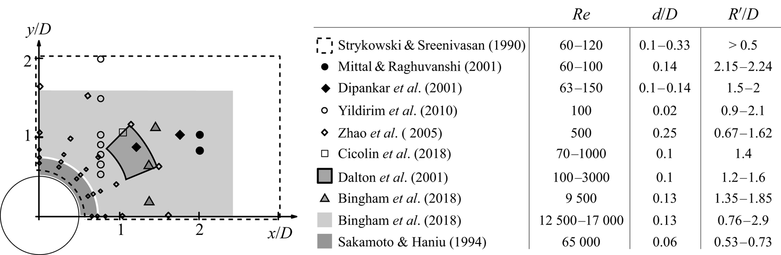
 $D$. Figure 2 is a compilation of past studies with one control rod for
 $90^{\circ }\leqslant \theta \leqslant 180^{\circ }$,
 $d/D<0.33$ and for a range of
 ${{\textit {Re}}}$ between 60 and 65 000. It shows the positions of control rods in the various studies illustrating the wide range of
 $R'/D$ that has been investigated.
Coordinate system.

Positions of the control rod in the range  $90^{\circ }\leqslant \theta \leqslant 180^{\circ }$ for different cases found in the literature.

The results of Dipankar, Sengupta & Talla (Reference Dipankar, Sengupta and Talla2007) and Mittal & Raghuvanshi (Reference Mittal and Raghuvanshi2001) agree with the findings of Strykowski & Sreenivasan (Reference Strykowski and Sreenivasan1990), and they found vortex-shedding suppression for low  ${{\textit {Re}}}$ and for similar values of
 $d/D$. Still in the range
 ${{\textit {Re}}}<100$ and for a smaller diameter of
 $d/D=0.02$, Yildirim, Rindt & Steenhoven (Reference Yildirim, Rindt and Steenhoven2010) did not observe complete vortex suppression, but found a significant attenuation of vortex strength. Dalton, Xu & Owen (Reference Dalton, Xu and Owen2001) performed numerical simulations in the range
 $100\leqslant {{\textit {Re}}}\leqslant 3000$ and with
 $d/D=0.1$, only observing complete suppression of vortex shedding at
 ${{\textit {Re}}}=100$. For
 ${{\textit {Re}}}=3000$, they reported a drag reduction of approximately
 $25\,\%$ when
 $R'/D=1.2$ and
 $\theta =160^{\circ }$. The fluctuating lift was also decreased, in their case by almost 85 %. These results confirmed that there is a significant
 ${{\textit {Re}}}$ dependency on the optimal position where the rod should be located. This was reinforced by the results of Cicolin et al. (Reference Cicolin, Serson, Assi and Meneghini2018), where the control rod was kept at a fixed position
 $(R'/D=1.4,\theta =135^{\circ })$ and
 ${{\textit {Re}}}$ was varied. It completely suppressed vortex shedding at
 ${{\textit {Re}}}=70$, attenuated the fluctuating forces at
 ${{\textit {Re}}}=200$ and had little effect at
 ${{\textit {Re}}}=1000$. At moderate values of
 ${{\textit {Re}}}=12\,500$ in the subcritical range, Bingham et al. (Reference Bingham, Raibaudo, Morton and Martinuzzi2018b) adopted a different approach and used an evolutionary algorithm to home in on the position of the control rod that minimised fluctuating lift on the main cylinder. The extensive area they covered for placing a control rod is shown shaded in figure 2. They concluded that fluctuating lift could be reduced by 90 % using a control rod with
 $d/D=0.125$, placed at
 $R'/D=1.31$ and
 $\theta =116^{\circ }$.
However, not all research on this topic has been limited to a circular cylinder as the bluff body. Parezanovic & Cadot (Reference Parezanovic and Cadot2012) performed a comprehensive study of the sensitivity of the wake past a D-shaped cylinder with one control rod. Their study included control rod diameters in the range  $d/H=0.04 \text {--} 0.12$, where in this case
 $H$ is the height of the base of the body. A significant difference between this study and many previous ones is that the separation points on the main body are not free to move. Nevertheless, they identified a number of flow states that have characteristics with some similarities to those found with a circular cylinder as the main body. According to the position of the control rod, they separated their results into different states. Sakamoto & Haniu (Reference Sakamoto and Haniu1994) visualised the flow in the wake of a circular cylinder with a single control rod using smoke and identified five different flow patterns. Their sketches of the flow indicate the importance of the proximity of the control rod to a free shear layer separating from the main cylinder. Returning to Parezanovic & Cadot (Reference Parezanovic and Cadot2012), they sketched four flow patterns in the wake of their D-shaped body with a single control rod. Their near-wake configurations are entitled external flow, outer shear, mid-shear and inner shear. The descriptions relate to the positions of the control rod relative to a free shear layer. Common to both of these studies, they found states that were bistable. Parezanovic, Monchaux & Cadot (Reference Parezanovic, Monchaux and Cadot2015) extended research on the D-shaped body to obtain more information on the bistability they had observed.
The present experiment-based investigation complements previous studies by providing further insight into the quintessential case of a circular cylinder with a single control rod. The main emphasis is on the fluid mechanisms involved rather than on optimising the effectiveness of this form of flow control. The Reynolds number,  $Re = 20\,000$, was in the subcritical range, well away from both the low-
 $Re$ regime and the onset of the drag crisis. In order to reduce the number of possible variables, the diameters of the main cylinder and the control rod were fixed, as was the distance between their centres. Previous works showed that when the rod and the cylinder have different orders of magnitude, the size of the rod is less relevant to the system's physics than its position, so we kept the ratio between the rod and the cylinder fixed,
 $d/D=1/10$. Past studies also revealed that there is a relationship between
 $Re$ and the sensitive regions for actuation. As
 $Re$ increases, the positions where the rod most affects the system gets closer to the cylinder. Besides, if the control rod is close to the cylinder surface it is more likely that there will be interactions with the cylinder boundary layer; hence
 $R'/D$ was fixed at
 $0.7$ giving a gap between the surfaces of the cylinder and control rod equal to
 $0.15D$. The important parameter that was varied was the angular position of the control rod,
 $\theta$, measured from the front stagnation line and moved from
 $90^{\circ }$ to
 $180^{\circ }$. This range of control rod angle was chosen as it is common to a number of previous studies as shown in figure 2.
As found by previous authors, the influence that a control rod has on the flow field around a bluff body depends on how the development of the shear layers separating from the body are affected by the presence of the control rod. With a single control rod it is the shear layer separating from the same side of the body as the rod that plays the most important role. By changing the angular position of the rod, the approaching shear layer has several possible paths. It may pass above the control rod or take a route between the cylinder wall and the control rod. Possibly the most challenging case is when the control rod is directly in the path of the shear layer and descriptions such as cutting and splitting the shear layer can be found in the literature. When the control rod is outside the path of the shear layer it is exposed to an approaching flow with a velocity of a similar magnitude to that of the main cylinder. In our experiments the ratio of the diameters of the control rod and main cylinder,  $d/D$, was fixed at 0.1 indicating a
 ${{\textit {Re}}}_d$ for the control rod of approximately 2000, which is well above the threshold for vortex shedding.
Following this introduction, § 2 details the experimental arrangement and methodology. Mean lift and drag forces were measured separately on the main cylinder and the control rod as well as on the combined system of main cylinder and control rod. The fluctuating forces were also measured but not separately for the control rod. Extensive particle image velocimetry (PIV) measurements were made and post-processed using an optimal mode decomposition (OMD)-based‘smart filter’ in order to have a clearer picture of the flow states and to be able to locate separation. In § 3, a diagnostic tool is presented that is used to identify the various flow states including a bistable state. Each state is described in detail calling on both the force and PIV data as well as animations derived from PIV. This is followed by a concluding section that lists new findings of the influence imposed on the flow around a circular cylinder by a control rod.
2. Experimental arrangement and methodology
Experiments were carried out in the recirculating water channel of the Department of Aeronautics at Imperial College London. The facility has a 0.6 m square test section and the length is 8.2 m. For all experiments the flow velocity was set at  $0.4\ \textrm {m}\ \textrm {s}^{-1}$ and at this speed the turbulence intensity is approximately 1.5 % at the position of the test cylinder. A thorough characterisation of the free-stream turbulence in this facility, including its two-point correlation, can be found in Baj & Buxton (Reference Baj and Buxton2017). The Froude number in these experiments was
 $Fr=U_\infty /\sqrt {gH}\approx 0.16$. Based on the studies of Reichl, Hourigan & Thompson (Reference Reichl, Hourigan and Thompson2005) and Bingham, Morton & Martinuzzi (Reference Bingham, Morton and Martinuzzi2018a), for
 $Fr<0.3$, we did not expected an influence of surface deformations on the flow dynamics. Two main sets of experiments were carried out: one was to measure hydrodynamic forces and the other was to investigate flow fields using PIV. The key properties relating to the experiments are provided in table 1 and the symbols used are depicted in figure 1.
Properties of models and experiments common to all campaigns.

2.1. Force measurements
For measuring forces the cylinder was attached to a load cell that was fixed above the water level. The load cell was an ATI Gamma IP68-SI-65-5 force transducer, capable of acquiring forces up to 65 N in the  $x$ and
 $y$ directions with a resolution of
 ${\pm }0.012$ N. The main cylinder was an acrylic tube with a diameter of
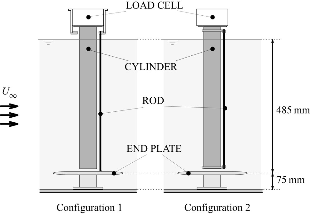
 $50$ mm and a wetted length of 485 mm, giving an aspect ratio of 9.7. Its upper end was connected directly to the load cell. In order to minimise end effects at the lower end of the cylinder, an end plate was fixed to the floor of the flume. The distance between the floor and the end plate was 75 mm and this is larger than the thickness of the boundary layer, which at this position was found to be approximately 35 mm. The gap between the cylinder and the end plate was kept less than 1 mm. The control rod was a carbon fibre tube with an outer diameter of 5 mm. Forces were acquired for two different arrangements for mounting the control rod, as shown in figure 3. In configuration 1, the rod's upper end was fixed in the outer shield of the load cell, whereas the lower end was fixed to the end plate. In this way, the load cell acquired the forces acting on the main cylinder only. In configuration 2, the rod was attached to the cylinder through two rings, allowing the load cell to acquire the forces acting on the combined system, i.e. the two bodies together. In both configurations, the end supports for the control rod kept the distance between it and the main cylinder constant along its length. The supports could be rotated around the cylinder, enabling different angular positions of the control rod to be set. The supports and the control rod were designed such that the deflection of the rod under hydrodynamic loading was negligible. The main quantities relating to the force measurements are given in table 2, where
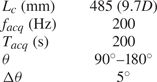
 $f_{acq}$ is the data acquisition rate,
 $T_{acq}$ is the acquisition time and
 $\Delta \theta$ is the increment for changing
 $\theta$.
Arrangement of the system for force measurements. Configuration acquiring the forces on the combined system (right) and only on the main cylinder (left).

Properties of the force measurement experiments.

The forces on the main cylinder were found from measurements made in configuration 1 and their dimensionless forms are given by
 \begin{equation} C_{D,L}^{{Cylinder}} = \frac{F_{D,L}^{{Conf.1}}}{\tfrac{1}{2} \rho U_\infty^{2} D L_c}, \end{equation}
where suffixes  $D,L$ refer to the drag and lift forces, respectively. We term the component of the hydrodynamic force acting in the
 $x$ direction to be the drag and the component acting in the
 $y$ direction to be the lift. The force coefficients for just the control rod were obtained by the difference between the time-mean forces in configurations 2 and 1:
 \begin{equation} {{C}_{D,L}^{Rod}} = \frac{({F}_{D,L}^{{Conf.2}}-{F}_{D,L}^{{Conf.1}})}{\tfrac{1}{2} \rho U_\infty^{2} D L_c}. \end{equation}
In addition to time-mean force coefficients, coefficients of the fluctuating forces acting on the cylinder and cylinder plus control rod were also found. However, it was not possible to deduce the fluctuating forces on the control rod and only its time-mean coefficients could be found.
2.2. Particle image velocimetry measurements
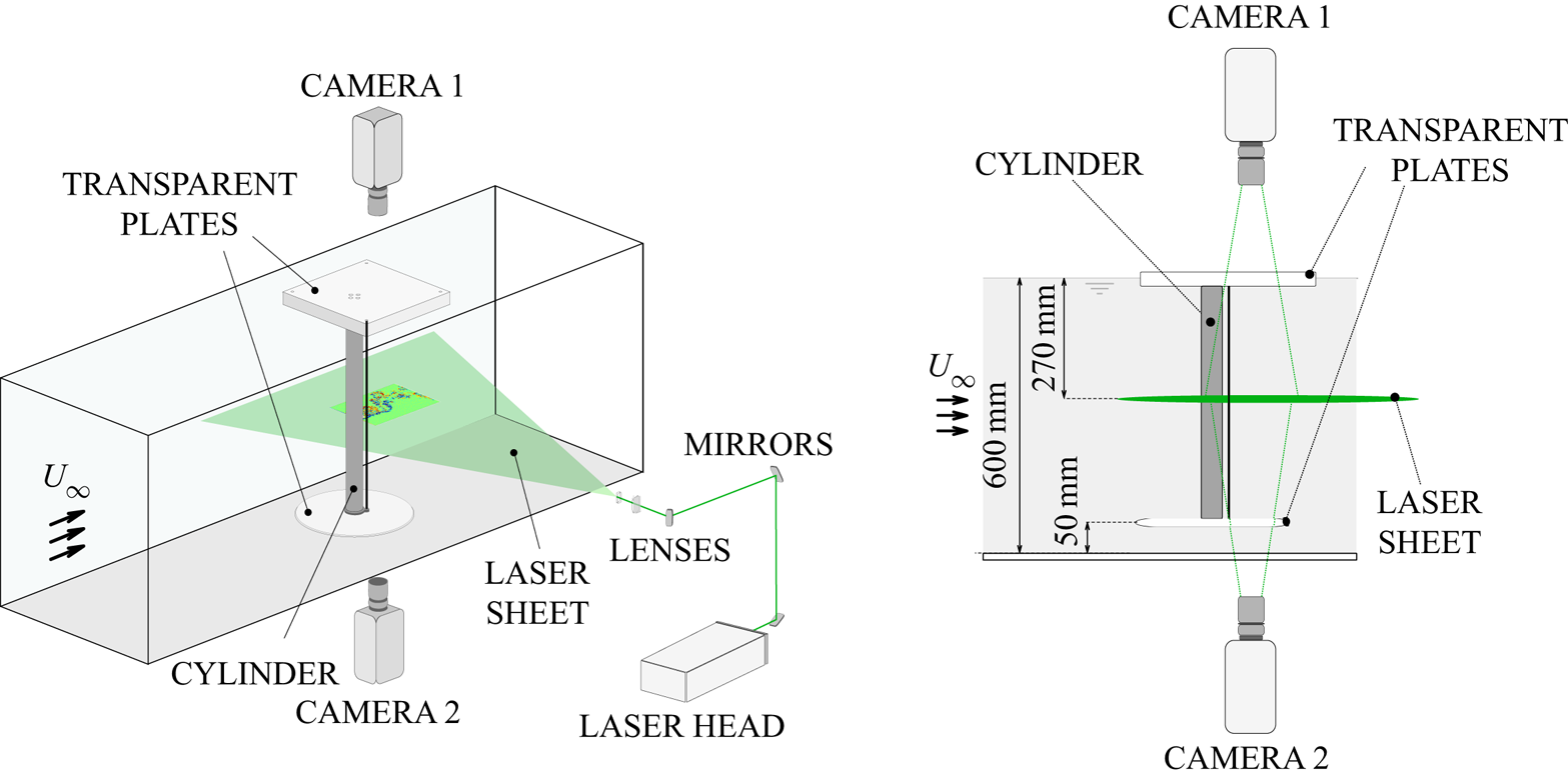
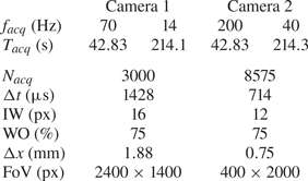
For PIV measurements the main cylinder was attached at its lower end to an acrylic disc with a diameter of 350 mm which acted as an effective end plate. The gap between the floor of the flume and the disc was fixed at 50 mm so that it was above the flume's boundary later. The top end of the main cylinder was attached to a square plate partially immersed in the water, as illustrated in figure 4. The control rod was fixed to the cylinder with supports similar to those used for the force measurements so as to keep the gap constant and to allow different angles to be set. The top and bottom plates were transparent to allow image recording, as shown in figure 4. As also illustrated in figure 4, PIV data were acquired at a plane located near the middle of the cylinder. The illumination source was a high-speed Litron LDY304 Nd:YLF laser, which operated at a constant frequency of 1400 Hz. An optical system formed by mirrors and lenses directed the laser beam through the channel's glass walls. The flow was seeded with polyamide particles with an average diameter of  $7\,\mathrm {\mu }\textrm {m}$. The acquisition of images was obtained using two cameras, one looking from the top of the model and the other from the bottom. Each camera was a Phantom v641 model with maximum resolution of
 $2460\times 1600$ px and internal storage memory for
 $5700$ images at the highest resolution. In order to capture simultaneously different scales of the flow, each camera focused on a different field of view (FoV), set by two lenses (Nikkon 70 mm
 $f=2:8$ and 105 mm
 $f=2:8$). The cameras operated at different acquisition rates, and their synchronisation with the laser pulses was controlled through an external pulse generator (Stanford DG645).
Arrangement of model, cameras and laser sheet in the flume.

The PIV measurements were also carried out at a flow velocity of  $0.4\ \textrm {m}\ \textrm {s}^{-1}$, yielding
 $Re=20\,000$. The angular position of the control rod (
 $\theta$) was varied from
 $90^{\circ }$ to
 $140^{\circ }$ with a
 $5^{\circ }$ step between consecutive cases and an average error of
 ${\pm } 1^{\circ }$. For each run, the flow was established by accelerating the flume from still water up to the desired velocity, and the acquisition started after the stabilisation of the flow. Table 3 summarises the main properties of the PIV set-up. The cameras acquired images in different regions of the flow for the same time period
 $T_{{acq}}$, which covered approximately 70 cycles of vortex shedding from the main cylinder. For certain cases, an additional run was recorded over a longer time period and with an acquisition frequency five times lower. Camera 1 focused on a FoV that captured a large part of the near wake, while camera 2 focused on two narrow strips (acquired in different runs), capturing smaller scales at an acquisition frequency higher than that of camera 1. The main purpose of recording with camera 2 was to provide longer time series. Figure 5 illustrates the FoV of each camera.
Properties of the PIV experiments.

Field of view for each camera.

The images were preprocessed and the flow fields calculated using the commercial software DaVis 8.4. The frequency of acquisition  $f_{{acq}}$ was set to be high enough to capture at least twice the frequencies of vortex shedding of the main cylinder and the control rod. Initially a Gaussian filter was applied to the PIV data followed by the subtraction of the mean local intensity with side 3 px. Every pixel then had its intensity confined between a minimum of 0 and a maximum of 2000 counts. These processes were carried out in order to smooth the image, mitigate the interference of the image background and prevent vector contamination by high-intensity peaks. Flow fields were calculated using a standard multi-pass cross-correlation method. The first step had a one-pass, 50 % window overlap (WO) and a 48 px interrogation window (IW) for all cases. The second and final pass had a different configuration for each camera. The main properties are presented in table 3, including the number of images (
 $N_{acq}$), the time interval between adjacent images (
 $\Delta t$) and the spatial resolution (
 $\Delta x$). As for post-processing, a universal outlier detector filter (Westerweel & Scarano Reference Westerweel and Scarano2005) with size
 $5\times 5$ px was applied to remove spurious vectors. For each case, the total number of replaced vectors was lower than 1 % of the total.
2.2.1. Post-processing
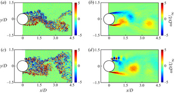
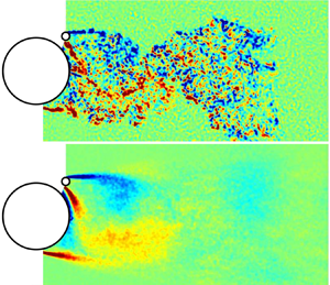
The processed velocity fields exported from DaVis had high spatial resolution, even those with the largest FoV. Each instantaneous field contained information on both coherent structures and fine-scale turbulent fluctuations. Since our main interest is focused on the former, we needed to process the velocity fields again in order to remove fluctuations less relevant to the large-scale dynamics of the system. The process adopted was a ‘smart filter’, understood as a filter capable of removing highly damped fluctuations regardless of their frequency or energy content. This is a key factor since the vortex shedding induced by the control rod is expected to be one order of magnitude higher in frequency than that of the main cylinder. Whilst these fluctuations are not especially energetic, they are dynamically important. We employed OMD, which is a method proposed by Wynn et al. (Reference Wynn, Pearson, Ganapathisubramani and Goulart2013) as a generalisation of the dynamical mode decomposition, first proposed by Schmid (Reference Schmid2010). The algorithm used was based on that provided by Wynn et al. (Reference Wynn, Pearson, Ganapathisubramani and Goulart2013) and is further described in Appendix A. An example of a previous application of such an OMD-based ‘smart filter’ to turbulent velocity data is given in Rodríguez-López, Bruce & Buxton (Reference Rodríguez-López, Bruce and Buxton2016). Figure 6 shows two examples of vorticity fields reconstructed using OMD: one is for the bare cylinder (the main cylinder without a control rod) and the other for a case with the cylinder and control rod. All instantaneous velocity and vorticity fields presented hereafter were processed using the same procedure. Time series and power spectra of velocity, however, were calculated from the original unfiltered fields.
Instantaneous vorticity fields: (a) bare cylinder and (c) case  $\theta =110^{\circ }$; and fields to which the smart OMD-based filtering has been applied: (b) bare cylinder and (d) case
 $\theta =110^{\circ }$.

3. Results and discussion
The placement of a rod in the range  $90^{\circ }\leqslant \theta \leqslant 180^{\circ }$ causes significant changes in the development of the wake. Based on the flow characteristics, and in common with previous research, angular positions are divided into groups associated with particular flow states, including one which is a bistable case. In order to identify the states, PIV was used to measure the tangential velocity component of the flow nearest to the midpoint,
 $P$, of the gap between the cylinder and the control rod,
 $v_t(P)$. This velocity proved to be very useful as a diagnostic tool. Figure 7(a) illustrates how the velocity is defined, and time series of
 $v_t(P)$ are shown in figure 7(b–h). In order to link flow states to the velocity traces, reference will be made to figure 8(a) which shows instantaneous vorticity and velocity fields for the three stable states observed in our investigation.
Time series of  $v_t(P)$ for different values of
 $\theta$. (a) Definition of
 $P$ and
 $v_t(P)$. (b) Angle
 $\theta =110^{\circ }$, State I; (c)
 $\theta =115^{\circ }$, State I; (d)
 $\theta =120^{\circ }$, State II; (e)
 $\theta =125^{\circ }$, State II; (f)
 $\theta =130^{\circ }$, bistable case; (g)
 $\theta =135^{\circ }$, State III; (h)
 $\theta =140^{\circ }$, State III.

Instantaneous vorticity (left) and velocity (right) fields for each of the three stable dynamical states characterised in this work. (a) State I;  $\theta =110^{\circ }$. (b) State II;
 $\theta =120^{\circ }$. (c) State III;
 $\theta =140^{\circ }$. Their development can also be seen in the supplementary movies available at https://doi.org/10.1017/jfm.2021.64.

For  $90^{\circ }\leqslant \theta \leqslant 115^{\circ }$ the time-mean value of
 $v_t(P)$ is close to the free-stream velocity and the fluctuating component has a dominant frequency equal to the shedding frequency of the main cylinder. Examples of the flow in this state, State I, are shown in figure 8(a), and it is characterised by the formation of distinct wakes, developed by the main cylinder and the control rod. Both wakes shed vortices but with very different frequencies and length scales. Moving to
 $\theta =120^{\circ }$ and
 $\theta =125^{\circ }$, an intense jet appears in the gap between the cylinder and the control rod, with
 $v_t(P)/U_\infty \approx 1.3$ and it is relatively steady, as seen in figures 7(d) and 7(e). This jet is a dominant feature of State II, as observed in figure 8(b). The third stable state, State III, was identified for
 $\theta =135^{\circ }$ and
 $\theta =140^{\circ }$. In this state the average value of
 $v_t(P)$ is close to zero, as shown in figures 7(g) and 7(h). The cylinder boundary layer separates sufficiently far upstream of the control rod for the free shear layer to pass above it, leaving point
 $P$ within the cylinder's recirculation zone. This state is illustrated in figure 8(c) and is characterised by the development of a vortex street wake, similar to the bare cylinder case. The velocity trace plotted in figure 7(f) for
 $\theta =130^{\circ }$ shows
 $v_t (P)$ varying over the range 0–1.5, and it is very different from those for the three stable states.This is an example from the state showing bistability.
Measurements of the variation of hydrodynamic force coefficients with  $\theta$ are shown in figure 9 together with an indication of the ranges of
 $\theta$ occupied by the flow states introduced above. The forces acting on the cylinder without a control rod, the bare cylinder, were measured first to serve as reference data. The results are a mean drag coefficient
 $\bar {C}_D=1.10$, a coefficient of fluctuating lift
 $C'_L=0.27$ and a Strouhal number
 $St=0.194$. These values are in close agreement with data to be found in works by Zdravkovich (Reference Zdravkovich1997) and Norberg (Reference Norberg2003). It should be noted that as well as Reynolds number the free-stream turbulence level has an effect on circular cylinder flow. For the parameters used in our investigation,
 $Re=20\,000$ and a free-stream turbulence level of 1.5 %, Fage & Warsap (Reference Fage and Warsap1929) reported a similar value of mean drag coefficient. Note that fluctuating forces are computed as the root-mean-square (r.m.s.) values acting on the full span. In figure 9, the bare cylinder values are denoted by a solid dark line.
(a) The r.m.s. of the fluctuating lift force on the cylinder (top) and the relative power spectral density (bottom) for the cases  $90^{\circ }\leqslant \theta \leqslant 180^{\circ }$. The solid lines represent the r.m.s. and the peak
 $St$ of
 $C_L^{\prime }$ for the bare cylinder case, respectively. (b) Average hydrodynamic force coefficients over the cylinder (top) and the control rod (bottom). (c) Average hydrodynamic force coefficients over the combined system. The solid grey line represents the mean drag coefficient of the bare cylinder case.

With the control rod in place, the mean lift and drag coefficients acting on it are also presented in figure 9(b), but note that all coefficients are calculated using the diameter of the main cylinder ( $D$) and the free-stream velocity. This makes it easier to compare the relative contributions of the main cylinder and control rod to the overall forces. With the addition of a control rod it can experience lift and drag forces on itself as well as influencing the forces acting on the main cylinder. Hence the total mean force coefficient has been calculated separately for the main cylinder and control rod. Mean drag, lift and total force coefficients for the combined system of cylinder and control rod are shown in figure 9(c).
In State I, comparing with the bare cylinder, the cylinder has a lower drag coefficient, a small but positive mean lift coefficient, a similar level of fluctuating lift and a Strouhal number increasing with increasing  $\theta$, but consistently lower than for the bare cylinder case. The control rod in State I is exposed to a velocity greater than the free-stream velocity and, depending on
 $\theta$, its drag ranges between 9 % and 14 % of the main cylinder's drag. Its lift force is negative and acts to offset a small amount of the lift on the main cylinder. Moving to State II, the mean drag on the cylinder falls by about 10 % with respect to the reference case; however, the mean lift increased so dramatically that the magnitude of the mean of the total hydrodynamic force acting on the cylinder was higher than for the reference case. The coefficient of fluctuating lift dropped to a minimum of
 $C'_L\approx 0.05$ at
 $\theta =120^{\circ }$, indicating an attenuation of vortex shedding and/or a reduction in its spanwise correlation. The corresponding power spectrum of the lift force did not have a prominent peak in the frequency range normally associated with vortex shedding, but scattered values in the range
 $0 < fd/U_\infty < 0.2$. The control rod exhibited positive values of both lift and drag in State II. For State III, the control rod is in the range
 $135^{\circ }\leqslant \theta \leqslant 180^{\circ }$ which places it in the recirculation region of the near wake of the main cylinder. The mean drag coefficient acting on the main cylinder and the Strouhal number have similar values to those of the bare cylinder. The mean lift coefficient was small and positive with values less than 0.1. As a result, the magnitude of the mean total force coefficient acting on the main cylinder was little different from the drag coefficient of the bare cylinder. With the control rod in the recirculation zone it experienced small negative drag and lift forces. It was in this state that the highest value of fluctuating lift on the main cylinder was recorded with
 $C'_L\approx 0.34$. These three flow states and the bistable case are analysed in more detail in §§ 3.1–3.4 and compared with findings of previous investigators.
3.1. State I
State I was observed for the cases with the control rod in the range  $90^{\circ }\leqslant \theta \leqslant 115^{\circ }$. Its main feature is the formation and interaction of the distinct wakes of the main cylinder and the control rod. Downstream this interaction results in a vortex street similar to that formed by a bare cylinder. The two shear layers from the main cylinder developed differently with the upper shear layer passing between the control rod and the main cylinder, as shown in figure 10. The sequence of instantaneous fields (and the supplementary movie) show that the upper boundary layer remains attached beyond the point where the gap between the two bodies is a minimum, up to a separation angle
 $\theta _{sep} > \theta$. The positions of the mean separation points, for various values of
 $\theta$, are shown in figure 11. Close agreement was found between separation points obtained from time-mean streamline patterns and from the mean tangential velocity component
 $\bar {v}_t$ measured at about 0.9 mm from the cylinder surface, separation being identified as the angular position at which
 $\bar {v}_t = 0$.
Vortex shedding cycle for the case  $\theta =110^{\circ }$, which is representative of State I. Vorticity fields are calculated from the smart-filtered velocity fields. Reynolds number
 ${{\textit {Re}}}=20\,000$. (a)
 $\phi =0$, (b)
 $\phi ={\rm \pi} /2$, (c)
 $\phi ={\rm \pi}$ and (d)
 $\phi ={3{\rm \pi} }/{2}$.

The  $\bar {v}_t$ fields for the cases bare cylinder and
 $90^{\circ }\leqslant \theta \leqslant 125^{\circ }$. The separation point (
 $\theta _{sep}$) was estimated using both the mean streamline patterns and the tangential velocity
 $\bar {v}_t$. It is estimated that
 $\theta _{sep}$ is accurate to within
 ${\pm }2^{\circ }$. (a) Bare cylinder; (b)
 $\theta =90^{\circ }$, State I; (c)
 $\theta =110^{\circ }$, State I; (d)
 $\theta =115^{\circ }$, State I; (e)
 $\theta =120^{\circ }$, State II; (f)
 $\theta =125^{\circ }$, State II.

The upper and lower boundary layer separation angles are shown plotted in figure 12 together with the cylinder drag coefficients for the range of  $\theta$ from
 $90^{\circ }$ to
 $135^{\circ }$. It is interesting to note that there is very little variation in the lower separation angle across the range of control rod placements. In contrast, separation of the upper boundary layer changes over a wide range of angles. In State I, figure 10 indicates that during a vortex shedding cycle the negatively signed vorticity of the cylinder's upper separated shear layer interacts with vortices shed from the control rod. Comparing with the bare cylinder case, this results in increased diffusion of the shear layer with negative vorticity. The interaction of the cylinder's top shear layer with the wake of the control rod can be readily observed in the supplementary movie.
Variation of mean drag coefficients and separation points with  $\theta$ (for which PIV data were available). The solid lines represent the mean drag coefficient and separation point of the bare cylinder case.

It is known for a bare cylinder that if  $\theta _{{sep}}$ moves further round its surface this results in a drag reduction, due to increased pressure recovery ahead of the separation points and hence an increase in the base pressure. This is illustrated in figure 12 where an increase in the upper surface separation angle is accompanied by a reduction in the drag coefficient, and vice versa. In State I we found that if the characteristic length used in the definition of drag coefficient was changed from
 $D$ to
 $D'$, where
 $D'$ is the vertical distance between the upper and lower separation points, a drag coefficient of 1.14 resulted, regardless of the control rod angle. This suggests that separation of the upper boundary layer is directly influenced by the adverse pressure gradient caused by the presence of the control rod. It should be noted that the upper boundary layer separates at an angle beyond the position of the control rod. This is compatible with the flow locally speeding up in the gap between the cylinder surface and the control rod and then decelerating. Studies have been carried out by Parezanovic & Cadot (Reference Parezanovic and Cadot2012) and Sakamoto, Tan & Haniu (Reference Sakamoto, Tan and Haniu1991) into the effect of control rods on the flow around bluff bodies with fixed separation points. In these cases there will be some variations in the flow mechanisms compared with our experiments where substantial changes in separation position are observed.
Figure 9(b) shows that for all values of  $\theta$ comprising State I there is a positive lift force on the cylinder and a negative lift force on the control rod. The signs of these forces are consistent with the upper cylinder boundary layer remaining attached until just beyond the control rod. In State I, figure 7 shows that the gap flow has a marked unsteady component due to vortex shedding from the main cylinder; see figure 8(a) and the supplementary movie.
It is observed that the frequency of vortex shedding in State I is lower than that found for the bare cylinder (figures 9a and 14). Figure 13 shows comparisons of mean velocity and vorticity fields between the bare cylinder and the case  $\theta =110^{\circ }$. A number of factors influence the shedding frequency including the distance between the separated shear layers and the flow velocity at their outer edges. Gerrard (Reference Gerrard1966) established that in addition the Strouhal frequency is influenced by both the vortex formation length and the lateral diffusion of vorticity within the shear layers. He quantified diffusion by defining a diffusion length related to shear layer thickness and argued that the greater the diffusion length the longer it takes for a vortex to form and hence the lower the Strouhal number. Also he reasoned that the longer the vortex formation length the greater the diffusion length as the shear layer has further to diffuse ahead of vortex formation. Considering a bare circular cylinder over a large
 ${{\textit {Re}}}$ range, it is found that where the drag coefficient falls it is accompanied by a rising Strouhal number, and vice versa. With a circular cylinder a reduction in drag coefficient is associated with the separation points moving further round the surface and the near wake becoming narrower. Roshko (Reference Roshko1954) developed the concept of a universal Strouhal number by using the velocity at the edge of the shear layers at separation as the characteristic velocity and the distance between the shear layers as the characteristic length. For a circular cylinder his analysis supports the finding that as the distance between the shear layers reduces the Strouhal number increases.
Mean velocity fields, where the grey points mark  $\max (\overline {v'^{2}}/U_\infty ^{2})$, for the cases (a) bare cylinder and (c)
 $\theta =110^{\circ }$ which is typical for State I. Mean vorticity fields for the cases (b) bare cylinder and (d)
 $\theta =110^{\circ }$.

Within State I, the Strouhal number and drag coefficient behave in a similar way to that for the bare cylinder with the increase in the separation angle with increasing control rod angle leading to a reduction in drag and an increase in vortex-shedding frequency. With the control rod at  $\theta = 90^{\circ }$ the value of the drag coefficient for the main cylinder is very close to that for the bare cylinder but in figure 14(a) the Strouhal number is significantly lower. Searching for a reason for this we followed previous researchers and made measurements of the vortex formation length. Earlier measurements have been based on a hot-wire traverse along the centreline of the wake to find the position of the maximum value of the r.m.s. of the longitudinal component of fluctuating velocity. We processed our PIV data to reproduce what a hot-wire probe would have measured. For the bare cylinder the vortex formation length was
 $1.29D$ and this is in good agreement with published data (Szepessy & Bearman Reference Szepessy and Bearman1992), and with the control rod at
 $\theta =110^{\circ }$ it increases to
 $1.68D$. Also the PIV data showed a thickening of the upper separated shear layer from the main cylinder caused by interaction with the control rod's wake. According to Gerrard (Reference Gerrard1966), together these changes will increase the diffusion length, leading to a reduction in the shedding frequency. However, for
 $\theta = 90^{\circ }$ the vortex formation length rather than increasing reduced slightly from the bare cylinder value. In the literature, vortex formation lengths have mainly been presented for bluff bodies that do not generate a mean lift force. Since in the presence of lift the cylinder wake is deflected at an angle to the free-stream velocity, this brings into question how vortex formation lengths should be defined. Since lift coefficients as large as 0.6 were generated in some cases it was decided not to present further measurements of vortex formation length. Parezanovic & Cadot (Reference Parezanovic and Cadot2009) point out the difficulty of predicting the vortex-shedding frequency of a bluff body using stability theory when separation points are free to move, such as on a circular cylinder. Using the wake of a bare circular cylinder as the base flow, the introduction of a control rod cannot be considered as a small perturbation if there are changes in boundary layer separation positions. Sakamoto & Haniu (Reference Sakamoto and Haniu1994) carried out experiments with a control rod at
 $Re=65 \,000$ and varied
 $\theta$ between
 $0^{\circ }$ and
 $180^{\circ }$ to find angular positions where the control rod was most effective at reducing fluid forces. In the range of control rod angles we classify as State I they also found that the Strouhal number at
 $\theta = 90^{\circ }$ was below the value for the bare cylinder. Also throughout the range of
 $\theta$ in State I the shedding frequency increased with increasing
 $\theta$ but remained below the value for the bare cylinder. They do not include reasons for this behaviour. States similar to State I can be found in the literature, for example the ‘free stream’ case reported by Bingham et al. (Reference Bingham, Morton and Martinuzzi2018a) at
 $Re = 9500$ with the control rod at
 $R'/D = 1.85$ and with
 $\theta =142^{\circ }$. Compared with their bare cylinder the mean drag coefficient dropped by
 $8\,\%$. As expected the Strouhal number increased and in their case it rose by almost
 $5\,\%$ indicating an interaction between the shear layer and the control rod and a change in where separation occurs. Parezanovic & Cadot (Reference Parezanovic and Cadot2012) performed a study with a bluff body with fixed separation points, a D-shaped cylinder. They present sketches of four flow fields that they observed depending on the position of the control rod. Their ‘outer shear’ configuration is the closest to our State 1 with a reduction in drag due to an increase in base pressure.
Comparison of the spectra between State I and the bare cylinder: (a)  $v$ at the point of
 $\max (\overline {v^{2}}/U_\infty ^{2})$ and (b) lift coefficient.

It is interesting to note that in the low- ${{\textit {Re}}}$ study by Strykowski & Sreenivasan (Reference Strykowski and Sreenivasan1990), the rod's wake did not develop vortex shedding, which would have made the interaction with the main cylinder shear layer different from the present study. Figure 15 shows in State I the spectrum of
 $v'$ along the line
 $x/D=1.0$. The peaks in
 ${fD/U_\infty \approx 0.2 }$ and
 ${ fD/U_\infty \approx 2.4}$ are due to the periodic vortex shedding of the main cylinder (
 $f_D$) and the control rod (
 $f_d$), respectively. Besides these, two other clear frequency signatures appeared, at
 $f_d\pm f_D$, with a well-defined spatial arrangement, as the highest frequency (
 $f_d+f_D$) resides between the wakes of the main cylinder and the control rod and the other (
 $f_d-f_D$) resides closer to the control rod's wake. Baj & Buxton (Reference Baj and Buxton2017) investigated the interactions between wakes produced by a multi-scale array of bluff bodies and identified the same spectral signature with the same spatial arrangement at the intersection of different-sized wakes. Although the geometries and
 $Re$ were different, the similarity between the spectra and their spatial configuration is remarkable, which suggests that the physical phenomena behind the interaction are also similar. They reported that these frequencies
 $f_d \pm f_D$ are associated with secondary modes, which are the result of nonlinear interactions between the primary shedding modes in close proximity to one another. These modes play an important role in feeding kinetic energy to the residual turbulent fluctuations (understood as
 $u^{\prime \prime }$ in the triple decomposition of a turbulent velocity field
 $u = \bar {u} + \tilde {u} + u^{\prime \prime }$ in which
 $\tilde {u}$ corresponds to the periodic component of the fluctuating velocity). These residual fluctuations in turn are responsible for the majority of the dissipation of turbulent kinetic energy during such multi-scale wake interactions.
(a) Spectra along  $x/D = 1.0$ for the case
 $\theta =90^{\circ }$. The dark lines represent the signatures of the vortex shedding of the main cylinder (
 $f_D$) and the control rod (
 $f_d$), as well as the secondary modes (
 $f_d \pm f_D$), showing their spatial distribution. (b) Spectrum at the point
 $(x/D;y/D)=(1.0;0.77)$ where the four modes coexist.

3.2. State II
State II was observed for control rod angles  $\theta =120^{\circ }$ and
 $125^{\circ }$. Its major feature is that separation of the upper boundary layer moves substantially further round the cylinder, as shown in figures 11(e) and 11(f). With the rod placed at
 $\theta =120^{\circ }$ and
 $125\,^{\circ }$,
 $\theta _{sep}=173^{\circ }$ and
 $182^{\circ }$, respectively. The relatively high-speed flow that develops between the control rod and the cylinder surface acts to energise the cylinder boundary layer which remains attached for a considerable distance. It is possible that transition to turbulent flow occurs in the main cylinder upper boundary layer leading to the delayed separation, but this could not be verified. The behaviour of the flow is an example of the Coandă effect and such a fully attached jet would not form on a bluff body with fixed separation points. However, the study of Parezanovic & Cadot (Reference Parezanovic and Cadot2012) for a D-shaped body revealed a related phenomenon whereby a straight jet penetrated into the near wake, replenishing fluid removed by entrainment by the free shear layers. In a diagram they show the jet entering the near wake just ahead of their control cylinder. As in our experiments this results in a reduction in drag. Following the large movement in the position of the upper separation point on the circular cylinder, the drag coefficient
 $\bar {C}_D$ decreased to
 ${\approx }0.98$, which is a reduction of 11 % below that of the bare cylinder, whereas
 $\bar {C}_L$ increased to
 ${\approx }0.55$. These changes result in the magnitude of the mean overall hydrodynamic force acting on the main cylinder being greater than the drag force acting on the bare cylinder. This highlights the danger of considering only the change in the mean drag when using a control rod as a passive flow-control device. However, in State II the control rod is effective in reducing fluctuating forces due to vortex shedding. The r.m.s. of the lift force on the main cylinder decreased significantly, especially for
 $\theta =120^{\circ }$ where
 $C'_L\approx 0.05$, which is more than 80 % lower than for the bare cylinder.
In this state, as well as a large change in the flow around the main cylinder, there is also a substantial change in the control rod's wake when compared with State I. As a result, the time-mean forces acting on the rod change. For  $\theta =125^{\circ }$,
 $\bar {C}_D\approx 0.02$, which is more than 80 % lower than the expected value of 0.1 if the rod was exposed to just a free stream. When considering these values note that all coefficients for the control rod have the main cylinder diameter,
 $D$, as the representative length scale. The lift force on the rod changes from being negative in State I to positive in State II with a lift-to-drag ratio close to 1.0.
Figure 16 shows a cycle of vortex shedding and illustrates how four shear layers interact to form the combined system's wake. Following separation of the upper boundary layer on the main cylinder it reaches the separated shear layer from the bottom of the cylinder in the vicinity of  $(x/D,y/D)\approx (0.75,-0.5)$. The jet flow draws down the lower shear layer from the control rod such that it also follows the contour of the main cylinder. The mixing of these three shear layers results in one diffused shear layer with positively signed vorticity. The drawing down of the lower shear layer from the control rod causes a very broad near wake to form with a large region of low-speed flow. It is assumed that the resulting pressure recovery in the wake of the control rod is responsible for its large drag reduction. The upper shear layer originating from the control rod with negatively signed vorticity interacts with the diffused lower main cylinder shear layer with positive vorticity to initiate vortex shedding. Visually the vortices forming in the combined system's wake appear weaker than those in State I which is compatible with the reduction in fluctuating lift.
Vortex shedding cycle for the case  $\theta =125^{\circ }$ which is representative of State II. Vorticity fields calculated from the smart-filtered velocity fields. Reynolds number
 ${{\textit {Re}}}=20\,000$. (a)
 $\phi =0$; (b)
 $\phi ={{\rm \pi} }/{2}$; (c)
 $\phi ={\rm \pi}$; (d)
 $\phi ={3{\rm \pi} }/{2}$.

Figure 17 presents the mean velocity fields for two cases in State II. As discussed above, the most striking features are the strong jet formed between the bodies and the long region of near-stagnant fluid in the wake of the control rod. Figures 11(e), 11(f), 16 and 17 clearly show that the upper boundary layer on the main cylinder remains attached up to  $\theta _{sep} \approx 180^{\circ }$. In contrast, the lower boundary layer separates at
 $\theta _{sep} \approx 100^{\circ }$. This marked asymmetry in the separation locations is responsible for the large mean lift coefficient which, as shown figure 9, is unique to State II. It is interesting to observe that in figure 17 there is a very large difference between the sizes of the two recirculation zones. Whereas in State I we discussed the flow in terms of the wakes of two bluff bodies, in State II the configuration appears closer to a single body with a passage through it that supplies fluid to the near wake resulting in a drag reduction.
Mean velocity fields, where the solid line is the contour  $\bar {u}/U_\infty =0$ and the grey diamonds represent the points where
 $v'/U_\infty$ is maximum. Cases (a)
 $\theta =120^{\circ }$ and (b)
 $\theta =125^{\circ }$ which are both representative of State II.

Figure 18(a) shows spectra of  ${v'}^{2} / U_\infty ^{2}$ at the point in the wake where it is maximum and also shows spectra of
 $C_L'$. The spectral peaks for State II cases are lower with respect to the bare cylinder case, particularly for
 $\theta = 120^{\circ }$. The flow patterns close to the rear of the main cylinder for
 $\theta = 120^{\circ }$ and
 $\theta = 125^{\circ }$, shown in figures 8(b) and 16, respectively, are similar but show differences a short distance further downstream. For
 $\theta = 125^{\circ }$ there is evidence of regular vortex shedding while for
 $\theta = 120^{\circ }$ the wake structure is less well organised and there is mixing of vorticities of opposite sign. Figure 8(b) shows that this mixing leads to lateral diffusion of the shear layers and an apparent lack of regular vortex shedding. This is also displayed in the supplementary movie for this case. The spectra plotted in figure 18 confirm the weakening of regular vortex shedding in State II as the angle of the control rod is reduced. They are also compatible with the observation that the lowest value of
 $C'_L$ was found in State II for
 $\theta = 120^{\circ }$. It is interesting to note in figure 19(a) that the time series of lift for
 $\theta = 120^{\circ }$ has a weak fluctuation at a frequency close to the vortex-shedding frequency for the bare cylinder. Hence, it cannot be concluded that vortex shedding has been totally suppressed but rather it has been substantially weakened.
Comparison of the spectra between State II and the bare cylinder. (a) Spectra evaluated at the  $\max (\overline {v'^{2}}/U_\infty ^{2})$ point for each case. (b) Spectra of lift force.

Time series of the forces of bare cylinder and cases in State II. (a) Lift and (b) drag.

In State II, the main cylinder's upper boundary layer appears to pass between the cylinder and the control rod and if there was a free shear layer there is no evidence of it having an impact on the control rod. A related state found in the literature is the Type D case reported by Sakamoto & Haniu (Reference Sakamoto and Haniu1994) at  ${{\textit {Re}}}=65\,000$. By measuring the time-averaged pressure distribution around the main cylinder they were able to identify a short separation bubble at the position on the cylinder closest to their control cylinder. Due to the presence of the shadow of the control rod it was not possible in our study to confirm for State II from PIV that a short separation bubble formed, but the possibility cannot be dismissed.
3.3. State III
State III is characterised by the control rod being positioned within the recirculation zone of the main cylinder and is found to occur for  $\theta \geqslant 135^{\circ }$ up to
 $\theta =180^{\circ }$. The prominent feature of State III is the von Kármán vortex street formed by the interaction between shear layers shed from the main cylinder in a form very similar to the bare cylinder case. Figure 20 shows a cycle of vortex shedding for the combined system with the control rod at
 $\theta =135^{\circ }$. The upper shear layer from the main cylinder passes above the control rod. After which it is drawn into the near wake and forms a vortex as it interacts with the separated shear layer originating from the boundary layer on the lower half of the main cylinder thereby forming a vortex street. In the figure, due to the shadow formed above the main cylinder, it is not possible to follow the path of the upper shear layer to the control rod. Evidence that the majority of the vorticity of negative sign in the upper shear layer has originated from the main cylinder is provided by the absence of vorticity of significant strength and opposing sign being shed from the lower half of the control rod. The reason for this is that the control rod is situated in a recirculation region where the fluid velocity is very low, as indicated in figure 7(g).
Vortex shedding cycle for the case  $\theta =135^{\circ }$ which is representative of State III. The vorticity fields are calculated after the application of the OMD-based smart filter to the velocity fields. Reynolds number
 ${{\textit {Re}}}=20\,000$. (a)
 $\phi =0$; (b)
 $\phi ={{\rm \pi} }/{2}$; (c)
 $\phi ={\rm \pi}$; (d)
 $\phi ={3{\rm \pi} }/{2}$.

In State III, the upper separation point on the main cylinder does not vary as significantly as in the previous two states. Figure 21 shows that with  $\theta =135^{\circ }$ the separation points remain close to those for the bare cylinder,
 $\theta _{sep}\approx 100^{\circ }$. The position of the upper separation point could not be measured for the other angles in State III due to the presence of the shadow of the rod in the PIV fields. However, we assume that the separation positions will not vary significantly for
 $\theta >135^{\circ }$ since as the angle increases the control rod moves further from the upper shear layer. This would explain why the force coefficients in State III remain relatively close to the values for the bare cylinder case.
The  $\bar {v}_t$ fields for the cases of (a) bare cylinder and (b)
 $\theta =135^{\circ }$ which is representative of State III. The separation point (
 $\theta _{sep}$) for each case was defined as described in the text.

The main effects due to the presence of the control rod in State III are related to changes in the near wake. Figure 22 shows the time-averaged velocity fields for the cases associated with State III. The recirculation length was extended in both cases when compared to the flow around the bare cylinder; it increased from  $1.25 D$ to
 $1.75 D$ and
 $1.39 D$ for the cases
 $\theta =135^{\circ }$ and
 $140^{\circ }$, respectively.
Mean velocity fields, where the grey points define  $\max (\overline {v'^{2}}/U_\infty ^{2})$, for the cases (a)
 $\theta =135^{\circ }$ and (b)
 $\theta =140^{\circ }$.

For  $\theta \geqslant 140^{\circ }$, the control rod had a limited effect on the development of the shear layer and hence on the wake as a whole. These results suggest that the primary effect of the control rod in this State III is to divert the top separated shear layer, thereby forcing the interaction further downstream relative to the bare cylinder. As for the control rod it is notable that it has a negative drag for all
 $\theta$ values tested, indicating that it is in a reversed flow within the near wake. As an interesting consequence, the total drag of the combined system, i.e. cylinder and control rod, is lower than for the bare cylinder for all cases investigated in State III.
3.4. Bistable case
Figure 7 reveals that States I, II and III yield distinctive time series for  $v_t(P)$, with a well-defined mean value and frequency of oscillation. Figure 7(f) shows
 $v_t(P)$ with the control rod at
 $\theta =130^{\circ }$ and it is clear that its characteristics are quite different from those for the other states. The trace switches between high (
 $v_t(P)/U_\infty \approx 1$) and low (
 $v_t(P)/U_\infty \approx 0$) velocity at time intervals that are significantly longer than those associated with the vortex shedding. Figure 23(a) presents an instantaneous vorticity field for
 $\theta = 130^{\circ }$ at a time instant for which
 $v_t(P)/U_\infty \approx 1$ whilst figure 23(b) presents an instantaneous vorticity field in which
 $v_t(P)/U_\infty \approx 0.1$. It is clear that there is a fundamentally different flow structure at the two time instants and the case
 $\theta = 130^{\circ }$ is a bistable case. Non-stable flow configurations have also been found in previous literature on controlling bluff-body wakes with control rods. Sakamoto & Haniu (Reference Sakamoto and Haniu1994) (
 ${{\textit {Re}}} = 65\,000$) observed a tristable case (in which their type D flow pattern resembles the current State II) and Parezanovic et al. (Reference Parezanovic, Monchaux and Cadot2015) identified a bistable phenomenon in the flow over a D-shaped cylinder with a leeward control rod.
Instantaneous vorticity fields and streamline patterns for  $\theta =130^{\circ }$: (a) state Bistable A,
 $v_t(P)/U_\infty \approx 0.1$; (b) state Bistable B,
 $v_t(P)/U_\infty \approx 1.0$. Switching between the states can be be viewed in the supplementary movie.

We will refer to the bistable states as Bistable A ( $v_t/U_\infty \approx 0$) and Bistable B (
 $v_t/U_\infty \gtrsim 1.0$). For Bistable A, the combined wake of cylinder and control rod develops a von Kármán vortex street. The vorticity field has features in common with those in State III. When Bistable A switches to Bistable B the velocity at point
 $P$ between the main cylinder and control rod increases significantly and a jet forms between the two bodies. When this happens the upper boundary layer on the main cylinder finally separates close to
 $\theta _{sep} \approx 180^{\circ }$, after which it interacts strongly with the separated shear layer originating from the bottom of the cylinder. This means that Bistable B is visually similar to State II. Close inspection of the streamline pattern in figure 23(b) indicates the possible presence of a short separation bubble forming on the main cylinder at an angular position close to that of the control rod. As previously stated, Sakamoto & Haniu (Reference Sakamoto and Haniu1994) observed a short separation bubble in their type D flow pattern at
 $Re = 65\,000$ whereas we are working at
 $Re = 20\,000$. However, the geometric parameters in the two studies are quite similar and it is plausible that the closeness of the control rod to the main cylinder surface plays an important role in the formation of a separation bubble. It is proposed that the reason for the switching back and forth between bistable states A and B is due to the formation and breakdown of a short separation bubble.
Previous studies have noted that placing the control rod in close proximity to the separating shear layer is very favourable for reduction of both drag and fluctuating lift. As highlighted by figure 9 the overall hydrodynamic force (on both the main cylinder and the combined system) is a minimum for the case  $\theta = 130^{\circ }$. For the cylinder only, the drag is slightly higher than in State II but the mean lift drops significantly from
 $\bar {C}_L\approx 0.5$ in State II to
 $\bar {C}_L\lesssim 0.1$ in the bistable case, yielding a total force coefficient of
 ${\approx }0.99$, more than 10 % lower than for the bare cylinder. Dalton et al. (Reference Dalton, Xu and Owen2001) found the greatest reduction of mean drag and fluctuating lift when the rod was placed in the middle of the shear layer (
 $R'/D= 1.2; \theta = 160^{\circ }; {{\textit {Re}}} = 3000$) and Bingham et al. (Reference Bingham, Morton and Martinuzzi2018a) reported a drag reduction of 15 % and attenuation of the r.m.s. of lift of 66 % for a rod placed in the middle of the shear layer, although further away from the cylinder (
 $R'/D=1.5; \theta =155^{\circ }; {{\textit {Re}}}= 9 500$). The wake patterns in those cases were stable and visually similar to Bistable B; however, in the present case Bistable B was never observed in stable isolation, only as one of two bistable states for
 $\theta = 130^{\circ }$. The time series and spectra of the forces over the main cylinder are presented in figure 24. The main peaks in the spectra at
 $fD/U_\infty \approx 0.2$ are related to vortex shedding, which occurs for both states. No characteristic frequency of switching could be observed in the signal as there is no distinct peak at a frequency lower than the vortex shedding. As for the rod, the average net force is very close to zero in the bistable case (
 $|\bar {C}_D |< | \bar {C}_L |<0.01$), as seen in figure 9(b). Since we did not measure the forces directly on the rod, there is no information about instantaneous values. Based on the average values, however, we consider that the level of the forces on the rod at Bistable A is similar to State III, producing negative drag and lift while Bistable B produces positive drag and lift, similarly to State II. We conclude that the switching between states is hence responsible for the minimal mean force magnitude on the rod.
Force measurements at  $\theta =130^{\circ }$. (a) Time series and (b) power spectral densities.

In order to acquire data on the switching process between bistable states, a second run was carried out with an acquisition period five times longer than the first. Whilst these two runs were acquired in nominally the same configuration ( $\theta = 130^{\circ }$) the apparatus was assembled from scratch for both runs, yielding a small uncertainty in the precise angular position of the control rod. Figures 25(a) and 25(b) show the probability density functions (p.d.f.s; top right-hand panels) of the time series of
 $v_t(P)$ (top left-hand panels) for the two runs. Both runs exhibit bistable behaviour with
 $v_t(P)$ varying from lower velocities, which characterise Bistable A, to high velocities typical of Bi stable B. However, the distribution of velocities for the two runs is different. The first run has a modal peak at
 $v_t(P) \approx 1.2$ whereas the distribution of the second is concentrated around
 $v_t(P) \approx 0$. A threshold of
 $v_t(P)/U_\infty =0.6$, which is equidistant from the modes of the p.d.f.s for the first and second runs, was thus defined to delimit Bistable A and Bistable B. The time series were divided into periods during which the flow resided in a particular state before switching. In total
 $N$ switches of state were recorded and these are displayed in the bottom panels of figures 25(a) and 25(b). In particular, the flow's residence time in a particular bistable state before switching is denoted by the grey bars. The blue lines show the cumulative mean residence times of the flow in each state, plotted on the right-hand axes. In the first run, the flow started in Bistable B for a period of
 $\approx 20U_\infty /D$ and then switched to Bistable A, where it remained for a period of
 $\approx 10U_\infty /D$ and so on. In total, the flow switched 12 times in the first run and 43 times in the second run. Considering
 $T_s=1/f_s$ as the period of one cycle of vortex shedding for the bare cylinder, the mean residence time in Bistable A was approximately
 $0.6 T_s$ in the first run and approximately
 $3T_s$ in the second run. The mean residence time in Bistable B was approximately
 $1.5T_s$ in the first run and
 $0.4T_s$ in the second run.
Time series and p.d.f. of  $v_t$ (top) and time duration of the two states in the bistable case (bottom). (a) First run and (b) second run, which is five times longer.

From the p.d.f.s and switching statistics we conclude that despite a nominally identical configuration of  $\theta = 130^{\circ }$ the two runs are biased towards different bistable states and the dynamics of the residence times/switching between the states behaves differently for each run. Further, we note that the mean residence time in the bistable states converges for both runs. Thus, we infer that the flows of the first and second runs are fundamentally different and not simply the result of unconverged statistics or unrepresentative sampling during the shorter of the two experimental runs. Considering that the system has a setting angle error of about
 ${\pm }1^{\circ }$, the position of the rod was likely subtly different between the two runs. This reveals the high level of sensitivity of the flow in the bistable case
 $\theta = 130^{\circ }$. This high level of sensitivity to the precise angular position of the control rod makes this configuration an ideal test case for high-fidelity computational fluid dynamics.
Figure 26(a) shows the spectra of  $v_t(P)$ for the two runs. In spite of their different time series, the spectra are quite similar, as no distinct frequency associated with state switching was found for either run. Instead, we observe that the spectra have close to a
 $-2$ slope at low frequencies. This is consistent with the rapid transitions between bistable states, resembling a step, having a random nature to their occurrence which gives rise to a low-frequency cut-off in the spectrum with a
 $-2$ power law (Grandemange Reference Grandemange2013). The spectra obtained from the time series of
 $v$ at
 $(x/D;y/D)=(1.5;0)$ revealed that the intensity of vortex shedding was higher in the second run, and its associated frequency was lower for the first run. These spectra can be explained by the observation that during the short run the flow spent more time in state Bistable B, in which the vortex-shedding process is weaker and its frequency lower than in state Bistable A, which is similar to State III.
Comparison of spectra between the two runs. (a) Power spectral density of  $v_t$ and (b) spectra of
 $v'$ at the point
 $(x/D;y/D)=(1.5;0)$.

4. Conclusions
Experiments were performed in a water channel using a circular cylinder with a control rod attached. The angular position of the rod was varied from  $\theta =90^{\circ }$ to
 $180^{\circ }$ while the Reynolds number of the circular cylinder was kept constant at
 ${{\textit {Re}}}=20\,000$. the other parameters held constant were the centre-to-centre spacing between the cylinder and the control rod,
 $R'/D=0.7$, and the ratio of diameters of the control rod and the cylinder,
 $d/D=0.1$. Flow-field measurements were made using PIV and fluid forces were obtained for the cylinder and the control rod. By measuring forces separately on the control rod valuable information was obtained about the local flow field to supplement the PIV data. In common with previous investigations, several distinct flow regimes were observed depending on the angular position of the control rod. Three stable flow states were identified in addition to a bistable case and it was observed that compared to the bare cylinder, changes in the positions of boundary layer separation took place. Some particularly large changes in separation angle were noted for the boundary layer on the same side of the cylinder as the control rod giving rise to substantial lift forces. A new method was devised for identifying the various flow states. Using PIV, the component of the flow velocity normal to a line between the centres of the cylinder and control rod was recorded at the midpoint of the gap between the bodies. Each flow state was found to have a characteristic value of the ratio of the local mean velocity to the free-stream velocity and a distinctive variation of velocity with time.
State I,  $\theta =90^{\circ }$ to
 $115^{\circ }$, is characterised by the formation of individual vortex street wakes from the cylinder and control rod. In common with other states there was very little movement of the separation position of the boundary layer on the side of the cylinder opposite to the control rod. In this state, separation of the upper boundary layer moved to just beyond the angular position of the control rod. There was no significant change in the drag of the main cylinder but it developed a small lift force. In State II,
 $\theta =120^{\circ }$ to
 $125^{\circ }$, there is a large delay in the separation of the cylinder boundary layer and an energetic jet forms that follows the contour of the main cylinder. While there is a reduction of about 10 % in the drag coefficient, a mean lift coefficient of about
 $\bar {C}_L\approx 0.55$ develops. As a result of the high lift the total mean force acting on the combined body of cylinder and control rod is greater that the mean drag on the bare cylinder. However, fluctuating lift was substantially reduced for
 $\theta =120^{\circ }$, with the r.m.s. of lift force fluctuations decreasing by more than 80 % due to the weakening of vortex shedding. Over the range
 $135^{\circ } \leqslant \theta \leqslant 180^{\circ }$, the control rod remains within the recirculation zone of the main cylinder and this is the main characteristic of State III. The separation points and the drag coefficient are close to those of the bare cylinder and with the control rod in the recirculation zone it experiences a small negative drag force.
A finding regarding the flow structure is that the free shear layer arising from separation of the upper boundary layer on the cylinder is deflected by the control rod and not split as observed by other investigators, where the control rod was placed relatively further from the main cylinder. In State I, the free shear layer passes between the cylinder and the control rod whereas in State III the free shear layer passes over the control rod. In State II, the boundary layer appears to remain attached until well after passing below the control rod, in a manifestation of the Coandă effect.
A bistable case exists for  $\theta =130^{\circ }$ where the flow switches between Bistable A, with characteristics very close to State III, and Bistable B, where there is delayed final separation, similar to State II. It was found that a small change in the control rod's angular position, of about
 ${\pm }1^{\circ }$, would influence the time that the flow was in one or other of states Bistable A and Bistable B. Further research is required to confirm that the instability is due to the formation and bursting of a separation bubble.
Supplementary movies
Supplementary movies are available at https://doi.org/10.1017/jfm.2021.64.
Funding
We gratefully acknowledge support of the RCGI Research Centre for Gas Innovation, hosted by the University of São Paulo and sponsored by FAPESP São Paulo Research Foundation (2014/50279-4) and Shell Brasil, and the support of ANP Brazil's National Oil, Natural Gas and Biofuels Agency through the R&D levy regulation. M.M.C. is grateful for the support of CNPq (201176/2018-1).
Declaration of interests
The authors report no conflict of interest.
Appendix A. Optimal mode decomposition
Dynamic mode decomposition (DMD) relies on the basic idea that there is a linear dependency, approximately constant throughout the sampling period, between successive velocity-field snapshots, which can be written as
 \begin{equation} \left.\begin{gathered} \boldsymbol{v}_{\boldsymbol{n}+\boldsymbol{1}} =\boldsymbol{\mathsf{A}}\boldsymbol{v}_{\boldsymbol{n}},\\ \boldsymbol{\mathsf{A}}\in \mathbb{R}^{p\times p}, \end{gathered}\right\} \end{equation}
where  $\boldsymbol {v}_{\boldsymbol {n}}$ is an arbitrary snapshot having length denoted by
 $p$, which corresponds to the total number of vectors in the PIV vector field, and
 $\boldsymbol {A}$ represents the underlying linear system. The DMD algorithm estimates the dynamic properties of
 $\boldsymbol {A}$ and its successful adaptation relies on having a sufficiently large ensemble of snapshots. Optimal mode decomposition estimates the properties of
 $\boldsymbol {A}$ by replacing it with its low-rank form
 $\boldsymbol {LML}^{\boldsymbol {T}}$ and solving an optimisation problem for both
 $L$ and
 $M$. For a series of
 $N$ snapshots, the problem becomes
 \begin{equation} \left.\begin{gathered}
\min\|[\boldsymbol{v}_{\boldsymbol{2}},\ldots,\boldsymbol{v}_{\boldsymbol{N}}]-
\boldsymbol{\mathsf{LML}}^{\boldsymbol{\mathsf{T}}}[\boldsymbol{v}_{\boldsymbol{1}},\ldots,
\boldsymbol{v}_{\boldsymbol{N}-\boldsymbol{1}}]\|^{2} \\
\boldsymbol{\mathsf{LL}}^{\boldsymbol{\mathsf{T}}}=\boldsymbol{\mathsf{I}}, \quad
\boldsymbol{\mathsf{L}}\in \mathbb{R}^{p\times r}, \quad
\boldsymbol{\mathsf{M}}\in \mathbb{R}^{r\times r}.
\end{gathered}\right\} \end{equation}
The OMD eigenvalues ( $\lambda ^{*}$) are then defined as
 \begin{equation} \lambda^{*}_n =\frac{\log{\lambda_n(\boldsymbol{\mathsf{M}})}}{\Delta t_{acq}}, \end{equation}
where  $\lambda _n(\boldsymbol{\mathsf{M}})$ are the eigenvalues of the matrix
 $\boldsymbol{\mathsf{M}}$ and
 ${\Delta t}_{acq}=1/f_{acq}$ is the period between two consecutive velocity fields. There is one OMD mode associated with each
 $\lambda ^{*}_n$:
 \begin{equation} \boldsymbol{\varPhi}^{*}_{\boldsymbol{n}} =\boldsymbol{\mathsf{L}}\boldsymbol{z}_{\boldsymbol{n}}, \end{equation}
where  $\boldsymbol{\mathsf{L}}\boldsymbol{z}_{\boldsymbol {n}}$ is an eigenvector corresponding to the eigenvalue
 $\lambda _n(\boldsymbol{\mathsf{M}})$. A low-order model (LOM) representation of the velocity fields is then given by
 \begin{equation} \boldsymbol{v}_{{LOM}} =\sum_{n=1}^{r}c_n\,\boldsymbol{\varPhi}^{{*}}_{\boldsymbol{n}}\,e^{\lambda^{{*}}_n}, \end{equation}
where  $c_n$ are the coefficients associated with the OMD modes. Further details of OMD/DMD methods can be found in Wynn et al. (Reference Wynn, Pearson, Ganapathisubramani and Goulart2013) and their use for extracting coherent modes in flows forced simultaneously by multiple bluff bodies at multiple different length scales in Baj, Bruce & Buxton (Reference Baj, Bruce and Buxton2015). The low-order representation of the velocity fields using OMD fields can be seen as a ‘smart’ dynamical filter, as it keeps the structures more relevant to the dynamics of the flow regardless of their energy content, i.e the velocities are not filtered in relation to their size or time scale but considering their dynamic relevance to the flow.