


1. Introduction
Rayleigh–Bénard convection (RBC), where the flow is heated from below and cooled from above, is a general paradigm of thermal convection and has attracted considerable attention over the past few decades (Grossmann & Lohse Reference Grossmann and Lohse2000; Niemela et al. Reference Niemela, Skrbek, Sreenivasan and Donnelly2001; Ahlers et al. Reference Ahlers, Grossmann and Lohse2009; Lohse & Xia Reference Lohse and Xia2010; Chillà & Schumacher Reference Chillà and Schumacher2012; Yeh Reference Yeh2023; Lohse & Shishkina Reference Lohse and Shishkina2023Reference Lohse and Shishkina2024). In the RBC system, uneven temperatures create density differences in the fluid, causing convection under the influence of field forces. Typically, the field force that drives buoyancy is gravity. However, more recently, centrifugal convection (CC) has shown promising results in enhancing convection strength in laboratory settings (Jiang et al. Reference Jiang, Zhu, Wang, Huisman and Sun2020; Wang et al. Reference Wang, Liu, Zhou and Sun2022b , Reference Wang, Liu, Lai and Sun2024), where a powerful centrifugal force, generated by strong mechanical rotation, replaces gravity. In such experiments, a sufficiently high Rayleigh number is achieved, and the thermal convection transitions into the ultimate regime.
In real-world natural environments and industrial applications, thermal convection often occurs under more complex conditions (Telford Reference Telford1967; Owen & Tang Reference Owen and Tang2015; Schumacher & Sreenivasan Reference Schumacher and Sreenivasan2020; Bhadra et al. Reference Bhadra, Shishkina and Zhu2024, Reference Bhadra, Shishkina and Zhu2025), requiring the consideration of many additional factors, such as rotation (Zhong et al. Reference Zhong, Stevens, Clercx, Verzicco, Lohse and Ahlers2009; Ecke & Shishkina Reference Ecke and Shishkina2023), shear (Goluskin et al. Reference Goluskin, Johnston, Flierl and Spiegel2014; Scagliarini et al. Reference Scagliarini, Gylfason and Toschi2014; Blass et al. Reference Blass, Zhu, Verzicco, Lohse and Stevens2020; Zhong et al. Reference Zhong, Wang and Sun2023), ratchet surfaces (Jiang et al. Reference Jiang, Zhu, Mathai, Verzicco, Lohse and Sun2018), magnetic fields (Yan et al. Reference Yan, Tobias and Calkins2021; Song et al. Reference Song, Shishkina and Zhu2024), porous media (Liu et al. Reference Liu, Jiang, Chong, Zhu, Wan, Verzicco, Stevens, Lohse and Sun2020), vibration (Wang et al. Reference Wang, Zhou and Sun2020; Guo et al. Reference Guo, Wu, Wang, Zhou and Chong2023), modulation (Yang et al. Reference Yang, Chong, Wang, Verzicco, Shishkina and Lohse2020), and so on. Among these, considering the time dependence of the driving force or boundary conditions is particularly important. Turbulent flows driven by time-dependent forcing are ubiquitous in both natural flows and industrial applications, such as blood pulsations, periodic pressure variations in the atmosphere, and rotational speed fluctuations in rotating machinery (Berger & Wille Reference Berger and Wille1972; Anderson & Gill Reference Anderson and Gill1975; Davis Reference Davis1976). In thermal convection, periodic forces alter the flow state of the system, which in turn affects the coherent structures and heat transfer efficiency.
Typical studies of periodically driven turbulence focus on pipe flow and Taylor–Couette flow, where the flow is driven by a pressure gradient and the rotating inner cylinder boundary with sinusoidal periodic variation, respectively (Womersley Reference Womersley1955; Walsh & Donnelly Reference Walsh and Donnelly1988; Barenghi & Jones Reference Barenghi and Jones1989; He & Jackson Reference He and Jackson2009; Verschoof et al. Reference Verschoof, Te Nijenhuis, Huisman, Sun and Lohse2018). The system’s response to the driving force is similar and is governed by the Womersley number, defined as
 \begin{equation} Wo=L^*\sqrt {\frac {2\unicode{x03C0} }{T^*\nu ^*}}, \end{equation}
where
 $L^*$
is the characteristic length scale of the system,
 $\nu ^*$
is the kinematic viscosity, and
 $T^*$
is the period of the oscillation. For a small Womersley number (
 $Wo\lt 1$
), which indicates a small length scale, a long period, and a large viscosity, the periodic boundary motion (or driven force) can be fully responded to. As the Womersley number increases, the flow is not able to follow the boundary motion, with a decreasing amplitude and an increasing phase delay. When the Womersley number becomes sufficiently large (
 $Wo\gt 10^2$
), the response amplitude vanishes and the periodic input hardly affects the flow any more (Verschoof et al. Reference Verschoof, Te Nijenhuis, Huisman, Sun and Lohse2018).
Periodically driven turbulence has also been introduced to the RBC system in several studies (Jin & Xia Reference Jin and Xia2008; Sterl et al. Reference Sterl, Li and Zhong2016; Wang et al. Reference Wang, Zhou and Sun2020; Yang et al. Reference Yang, Chong, Wang, Verzicco, Shishkina and Lohse2020). Yang et al. (Reference Yang, Chong, Wang, Verzicco, Shishkina and Lohse2020) studied the RBC with a periodically heated lower plate, finding that the heat transfer efficiency first increases and then decreases with increasing frequency. They revealed that this behaviour is determined by the scales of the Stokes thermal boundary layer in relation to the thermal and viscous boundary layers of the system. What if there is an oscillating plate generating a Stokes viscous boundary layer? As the oscillating boundary motion can interact with the large-scale circulation (LSC), its effect on heat transfer may be more complicated. However, in traditional RBC, compared to oscillating temperature boundary conditions, it is challenging to generate oscillating velocity boundary conditions due to the limitations of the sidewall. Wang et al. (Reference Wang, Zhou and Sun2020) introduced horizontal vibration to RBC, producing a laterally oscillating buoyancy that affects heat transfer only at high frequencies. Liu et al. (Reference Liu, Jia, Li and Zhong2023) replaced the sidewalls with periodic boundaries in planar RBC, with only the hot boundary oscillating. This set-up resulted in an oscillating imposed shear due to the velocity difference between the two boundaries. As their study primarily focuses on the effect of oscillating velocities, the results resemble those of sheared convection (Goluskin et al. Reference Goluskin, Johnston, Flierl and Spiegel2014; Scagliarini et al. Reference Scagliarini, Gylfason and Toschi2014; Blass et al. Reference Blass, Zhu, Verzicco, Lohse and Stevens2020; Zhong et al. Reference Zhong, Wang and Sun2023), where heat transfer is suppressed in the buoyancy-dominated regime and enhanced in the shear-dominated regime.
Therefore, in this paper, we focus on the CC system, where convection occurs between cooled inner and heated outer cylinders under rapid solid-body rotation. In this high-speed rotating system, when the angular velocity changes, the boundaries oscillate in the rotating reference coordinate system. Since the azimuthal direction of the system is periodic, a circumferential flow occurs due to inertia. An interesting question is how the response flow interacts with the thermal flow and further influences heat transfer. This is the main focus of our paper.
The rest of the paper is organised as follows. The establishment of the numerical model and the direct numerical simulations are introduced in § 2, and the main results are discussed in § 3. Then in § 4, we provide a theoretical model. Finally, conclusions are presented in § 5.
2. Numerical model
A three-dimensional CC system in cylindrical coordinates
 $(r,\varphi ,z)$
is illustrated in figure 1. The incompressible viscous fluid is bounded by a cold inner cylinder with radius
 $r_i^*$
, and a hot outer cylinder with radius
 $r_o^*$
, co-rotating about the
 $z$
-axis at a periodic angular velocity
 $\Omega ^*(t^*)$
. The gap between the two cylinders is
 $L^*=r_o^*-r_i^*$
;
 $\theta ^*_{i,o}$
is the temperature of inner and outer cylinders, respectively, and the temperature difference is
 $\unicode{x1D6E5} ^*=\theta ^*_o-\theta ^*_i$
. Some fluid properties, including the coefficient of thermal expansion
 $\alpha ^*$
, the kinematic viscosity
 $\nu ^*$
, and the thermal diffusivity
 $\kappa ^*$
, are assumed to be constant in the system. Here, we consider that the angular velocity fluctuates sinusoidally around the mean value, which can be expressed as
 \begin{equation} \Omega ^*(t^*)=\Omega ^*_0(1+f(t^*)),\quad f(t^*)=e \sin(2 \unicode{x03C0} t^*/T^*), \end{equation}
where
 $\Omega ^*_0$
is the mean angular velocity,
 $T^*$
is the dimensional period, and
 $\Omega ^*_0e$
is the amplitude. As the angular velocity fluctuates, the centrifugal force varies as well. Therefore, to control the centrifugal force without drastic changes, we attempt to satisfy
 $e\ll 1$
in this study.
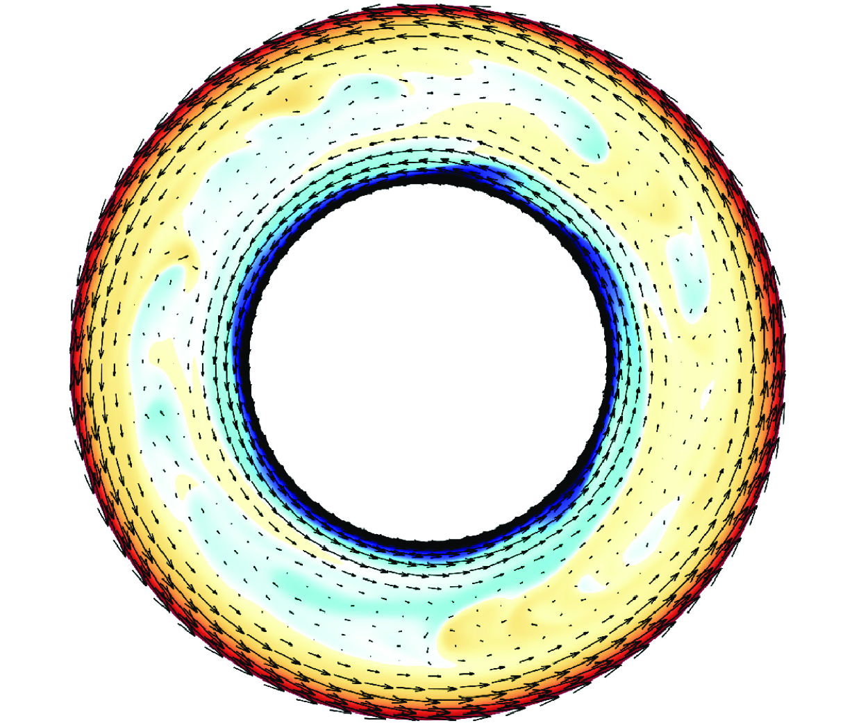
Schematic diagram of the flow configuration in the stationary reference frame, where
 $r_{i,o}^*$
and
 $\theta _{i,o}^*$
are the radius and temperature of the inner and outer cylinders, respectively. The system rotates at a time-dependent angular velocity
 $\Omega ^*(t)=\Omega _0^*(1+e \sin(2\unicode{x03C0} t^*/T^*))$
, and
 $L^*=r_o^*-r_i^*$
is the gap between the two cylinders.

For simplification, we analyse the system in a rotating reference frame at constant angular velocity
 $\Omega ^*_0$
. Hence the oscillation of angular velocity is manifested as periodic motions of the boundaries, i.e.
 \begin{equation} \begin{aligned} \text{for }r&=r_i^*,\quad u^*_\varphi =\Omega ^*_0r_i^*f(t^*),\\[3pt] \text{for }r&=r_o^*,\quad u^*_\varphi =\Omega ^*_0r_o^*f(t^*). \end{aligned} \end{equation}
2.1. Governing equations
In CC, the fluid is heated at the outer wall and moves to the inner wall driven by centrifugal buoyancy. The free-fall velocity is defined by the mean centrifugal acceleration as
 $U^*=\sqrt {\alpha ^*\unicode{x1D6E5} ^*L\Omega ^{*2}_0(r_i^*+r_o^*)/2}$
. With the gap
 $L^*$
, free-fall velocity
 $U^*$
, and temperature difference
 $\unicode{x1D6E5} ^*$
introduced as the length, velocity and temperature scales, respectively, the non-dimensional governing equations under the Oberbeck–Boussinesq assumption read (Jiang et al. Reference Jiang, Zhu, Wang, Huisman and Sun2020; Zhong et al. Reference Zhong, Wang and Sun2023)
 \begin{equation} \begin{aligned} \boldsymbol {\nabla } \boldsymbol{\cdot} \boldsymbol {u}&=0,\\[6pt] \frac {\partial \boldsymbol {u}}{\partial t}+\boldsymbol {u} \boldsymbol{\cdot} \boldsymbol {\nabla u}=-\boldsymbol {\nabla } p-Ro^{-1}\,\boldsymbol {e}_z\times \boldsymbol {u}&+\sqrt {\frac {Pr}{Ra}}\,{{\nabla }^2}\boldsymbol {u}-\theta \frac {2(1-\eta )}{1+\eta }\left(1+\frac {2u_\varphi }{Ro^{-1}r}\right)^2\boldsymbol {r},\\[6pt] \frac {\partial \theta }{\partial t}+\boldsymbol {\nabla } \boldsymbol{\cdot} (\boldsymbol {u}\theta )&=\sqrt {\frac {1}{Ra\, Pr}}\,{\nabla }^2 \theta ,\\ \end{aligned} \end{equation}
where
 $\boldsymbol {u}=(u_r,u_\varphi ,u_z)$
is the velocity vector,
 $p$
is the pressure (the density is contained within),
 $\theta$
is the temperature,
 $\boldsymbol {e}_z$
is the unit vector in the axial direction, and
 $\eta =r^*_i/r^*_o$
is the radius ratio. Three dimensionless parameters appearing in the governing equations are the Rayleigh number
 $Ra$
, the inverse Rossby number
 $Ro^{-1}$
, and the Prandtl number
 $Pr$
, which read
 \begin{equation} Ra=\frac {\alpha ^*\unicode{x1D6E5} ^*{L^*}^3\Omega _0^{*2}(r_i^*+r_o^*)/2}{\nu ^*\kappa ^*}, \quad Ro^{-1}=\frac {2\Omega ^*_0L^*}{U^*},\quad Pr=\frac {\nu ^*}{\kappa ^*}. \end{equation}
Moreover, the non-dimensional boundary conditions read
 \begin{equation} \begin{aligned} \text{for }r&=r_i,\quad \boldsymbol {u}=\left(0,\frac {Ro^{-1}}{2}r_if(t) ,0\right),\ \theta =0,\\ \text{for }r&=r_o,\quad \boldsymbol {u}=\left(0,\frac {Ro^{-1}}{2}r_of(t),0\right),\ \theta =1, \end{aligned} \end{equation}
where
 $r_{i,o}=r^*_{i,o}/L^*$
are the non-dimensional radii, and
 $f(t)=e \sin(2\unicode{x03C0} t/T)$
is the oscillation factor with the non-dimensional oscillation period
 $T=T^*U^*/L^*$
. Following (1.1), the Womersley number can be expressed by the non-dimensional parameters above:
 \begin{equation} Wo=(Ra/Pr)^{1/4}\sqrt {2\unicode{x03C0} /T}. \end{equation}
Therefore, there are five key control parameters of the system: the Rayleigh number
 $Ra$
(measuring the buoyancy-driving strength), the inverse Rossby number
 $Ro^{-1}$
(measuring Coriolis effects), the Prandtl number
 $Pr$
(fluid property), oscillation amplitude
 $e$
, and the non-dimensional oscillation period
 $T$
(or the Womersley number
 $Wo$
). As we aim to figure out the effect of oscillating boundaries, the oscillation amplitude
 $e$
and period
 $T$
are mainly concerned in the present work.
2.2. Parameter space
When the rotation velocity oscillates, there are several typical effects on the flow. First, due to inertia, it is difficult for the fluid in the bulk region to follow the boundary motion, thus a shear flow in the azimuthal direction is generated; this is the effect on which we focus in the present paper. Meanwhile, changes in rotational velocity can lead to fluctuations in centrifugal force, which can further influence the buoyancy strength. In the governing equations (2.3), the last term on the right-hand side of the momentum equation represents the effect of azimuthal motion on buoyancy. Considering that the boundary oscillation effect is strongest at the inner and outer walls, we substitute (2.5) into the buoyancy term and obtain that the centrifugal buoyancy at the boundary oscillates with a relative amplitude
 $(1+e)^2$
. Hence a relatively small
 $e$
is required to weaken the oscillating buoyancy. Taking into account that the heat transfer of the CC system is highly robust to the inhomogeneous distribution of buoyancy (Jiang et al. Reference Jiang, Zhu, Wang, Huisman and Sun2020), coupled with the need for a wide range of simulation parameters, we appropriately liberalise the restriction on the amplitude and take
 $e\in [0.01,0.2]$
. Subsequent results in § 3 have also demonstrated that the cases with slightly higher amplitudes have a consistent pattern of effect on heat transfer.
In addition, strong vibration can also induce buoyancy, which may transit the system into a thermal vibrational convection system (Wang et al. Reference Wang, Zhou and Sun2020; Wu et al. Reference Wu, Wang, Chong, Dong, Sun and Zhou2022; Guo et al. Reference Guo, Wu, Wang, Zhou and Chong2023). In traditional RBC, the heat transfer efficiency is able to be enhanced significantly up to
 $600\,\,\%$
by strong vibration (Wang et al. Reference Wang, Zhou and Sun2020). The introduced control parameter, termed the vibrational Rayleigh number, is defined as
 \begin{equation} Ra_{vib}=\frac {(\alpha ^*\unicode{x1D6E5} ^*L^*\Omega _0^*(r_i^*+r_o^*)e/2)^2}{2\nu ^*\kappa ^*}=2\left (\frac {e}{Ro^{-1}}\right )^2Ra. \end{equation}
The expression for
 $Ra_{vib}$
here is independent of the oscillation period
 $T$
, different from that in vibrational RBC, because the oscillating velocity amplitude is controlled rather than the displacement amplitude. According to the range of
 $e$
, we can find
 $Ra_{vib}\ll Ra$
. Thus in our parameter space, the buoyancy effect due to vibrations can always be neglected (Wang et al. Reference Wang, Zhou and Sun2020).
In CC experiments, the effect of gravity is always present. Jiang et al. (Reference Jiang, Zhu, Wang, Huisman and Sun2020) conducted experiments and numerical simulations, finding that the experimental and numerical results agree well at large centrifugal acceleration. This indicates that gravity can be neglected when centrifugal acceleration is much greater than Earth’s gravity. Furthermore, Yao et al. (Reference Yao, Emran, Teimurazov and Shishkina2025) performed a detailed simulation study on the effects of gravity. Their results show that strong gravity at a low system rotation rate induces vertical convection and makes the flow three-dimensional, while its influence can be ignored in the centrifugal buoyancy-dominated regime at large Froude numbers and
 $Ro^{-1}$
. The effect of Earth’s gravity on oscillating boundaries in CC is expected to be similar to its effect on CC itself, but a systematic investigation is needed in future studies. In the present work, the effect of Earth’s gravity is neglected.
Referring to our previous studies on CC (Jiang et al. Reference Jiang, Zhu, Wang, Huisman and Sun2020; Zhong et al. Reference Zhong, Wang and Sun2023), and considering computational costs, we fix
 $Ra=10^7$
,
 $Pr=4.3$
,
 $Ro^{-1}=20$
and
 $\eta =0.5$
. To highlight the effects of boundary motion and investigate the effects of oscillation amplitude and period, an oscillation amplitude range
 $e\in [0.01,0.2]$
and a wide oscillation period range
 $T\in [10^{-1},5\times 10^3]$
are chosen in the present study.
Check of grid resolution and flow two-dimensionalisation at the fixed parameters
 $Ra=10^7$
,
 $Pr=4.3$
and
 $Ro^{-1}=20$
. Here,
 $e$
and
 $T$
are the oscillation amplitude and period,
 $N_r, N_\varphi , N_z$
indicate the resolutions in the radial, azimuthal and axial directions, respectively,
 $\Gamma =H^*/L^*$
denotes the aspect ratio,
 $Nu$
denotes the Nusselt number, and
 $\epsilon _{Nu}$
denotes the relative error of
 $Nu$
, which is the difference between
 $Nu$
values averaged by the first and last halves of the simulation time.

2.3. Direct numerical simulations
A series of direct numerical simulations (DNS) are performed to study this problem. The governing equations (2.3) are solved on a Chebyshev-clustered staggered grid by an energy-conserving second-order finite-difference code AFiD. The time advancing employs a fractional-step third-order Runge–Kutta scheme, incorporating implicit terms derived from a Crank–Nicolson scheme. The code is widely used and strongly validated in previous simulations of RBC, Taylor–Couette flow and plane-Couette flow (Verzicco & Orlandi Reference Verzicco and Orlandi1996; van der Poel et al. Reference van der Poel, Ostilla-Mónico, Donners and Verzicco2015; Zhu et al. Reference Zhu2018). Considering that high-frequency oscillations may require higher resolution, we conducted a grid refinement check for different oscillation periods
 $T$
, referencing the previous grid resolutions on CC (Jiang et al. Reference Jiang, Wang, Liu and Sun2022; Zhong et al. Reference Zhong, Wang and Sun2023), with the results presented in table 1. Meanwhile, as the flow in CC is quasi-two-dimensional due to the strong rotation, a test of whether or not the flow is two-dimensional under oscillations is performed for different
 $T$
. In the parameter space of the present study, the flow is shown to remain quasi-two-dimensional, and the results of heat transfer are shown in the table 1 as well. Moreover, the Courant–Friedrichs–Lewy (CFL) conditions are taken as
 $\textit{CFL}\leqslant 0.7$
to guarantee computational stability (Ostilla et al. Reference Ostilla, Stevens, Grossmann, Verzicco and Lohse2013; van der Poel et al. Reference van der Poel, Ostilla-Mónico, Donners and Verzicco2015). Enough simulation time is ensured to limit the error in the statistics after the cases have reached the statistically stationary state. More numerical details are illustrated in Appendix A.
3. Results and discussion
3.1. Heat transfer
Figure 2(a) shows how the Nusselt number
 $Nu$
varies with the oscillation period
 $T$
and the velocity oscillation amplitude
 $e$
. When the system oscillates at a high frequency
 $T=0.1$
, there is no significant change in heat transfer efficiency due to the oscillation, and the heat transfers at different amplitudes are relatively similar. As the oscillation period increases, the heat transfer is suppressed gradually until it reaches the minimum at
 $T_{opt}\sim O(10)$
. Afterwards, as the oscillation period continues to increase,
 $Nu$
rises again until it returns to its original value of the non-oscillation case. Meanwhile, the degree of suppression of heat transfer by oscillations is highly correlated with the velocity oscillation amplitude
 $e$
. For a small value
 $e=0.01$
, the oscillation gives maximum suppression only
 $10\,\%$
. The
 $Nu$
value is first affected at
 $T\approx 5$
, and recovers at
 $T\approx 200$
, implying a narrow period range for which the oscillation has an effect. For a large value
 $e=0.2$
, nearly
 $87\,\,\%$
suppression of
 $Nu$
is achieved;
 $Nu$
has not recovered to the original value even at
 $T=5\times 10^3$
, which is the end of our parameter range. It is surprising that a low-frequency oscillation can give such a large inhibition on heat transfer with a
 $20\,\,\%$
oscillation amplitude of the rotating velocity. The result is not consistent with the discovery of Wang et al. (Reference Wang, Zhou and Sun2020) on the thermal vibration convection, in which only a high-frequency vibration can have an impact on the heat transfer of RBC. This conflict indicates the importance of sidewalls in vibration systems, because the sidewalls prevent the formation of zonal flow.
(a) The variation of
 $Nu$
with the oscillation period
 $T$
at various oscillation amplitudes
 $e$
. The red dashed line denotes the location of minimum
 $Nu$
for
 $e\geqslant 0.05$
. (b) The variation of the normalised Nusselt number
 $Nu/Nu_0$
with the Womersley number
 $Wo$
at various oscillation amplitudes
 $e$
. Here,
 $Nu_0$
is the Nusselt number of CC without oscillation.

The zonal flow formed by the oscillating boundaries is highly relevant to the periodically driven turbulence, which is described in the Introduction. Therefore, we replace the oscillation period
 $T$
by the Womersley number
 $Wo$
defined in (2.6), and the results are shown in figure 2(b). In the converted parameter space, it can be seen that oscillation affects the heat transfer mainly on
 $10^0\leqslant Wo \leqslant 10^2$
, which is consistent with the effective Womersley number range on periodically driven Taylor–Couette flow (Verschoof et al. Reference Verschoof, Te Nijenhuis, Huisman, Sun and Lohse2018). From the perspective of periodically driven turbulence, for an extremely small
 $Wo$
, the oscillation period is long, and the characteristic time of the oscillating system is much larger than the characteristic time of the convection, therefore such a slow change can hardly affect convection; for an extremely large
 $Wo$
, the oscillation period is short, and the characteristic length of oscillation is much smaller than the length scale of the convection system, thus it remains difficult for oscillations to influence the internal flow.
This scale analysis is consistent with that in RBC with periodically modulated thermal boundaries as well (Yang et al. Reference Yang, Chong, Wang, Verzicco, Shishkina and Lohse2020), where both high-frequency and low-frequency modulations influence the heat transfer little. However, when the thermal boundaries are periodically modulated, the heat transfer of the RBC system is enhanced, while in our system, when the velocity boundaries are periodically modulated, the heat transfer is suppressed. How does the oscillation inhibit the convection? This is what we need to address in the next subsection.
3.2. Typical suppressed convection under oscillation
To explore the inhibitory effect of oscillations on heat transfer, we examine a typical case near the minimum
 $Nu$
at
 $T=100$
and
 $e=0.05$
. Our focus will be on analysing the evolution of the flow structure throughout the oscillation period. Typical snapshots of the instantaneous temperature and velocity fields at different moments of one period after the convection is fully developed are shown in figures 3
(a–d). The corresponding time and instantaneous
 $Nu$
are marked by the vertical dashed lines in the
 $Nu$
versus
 $t$
plot in figure 3
(e).
The time evolution for the case with
 $T=100$
,
 $e=0.05$
. (a–d) Typical snapshots of the instantaneous temperature and velocity fields at different moments of one period: (a)
 $t=0$
, (b)
 $t=T/8$
, (c)
 $t=3T/8$
, (d)
 $t=T/2$
. The contour denotes the temperature distribution, and the vectors denote the velocity. (e) The Nusselt numbers vary with time during two periods. The four vertical dashed lines denote the moments of (a–d), respectively. (f) The azimuthally averaged azimuthal velocity
 $\langle u_\varphi \rangle _\varphi$
varies with time during two periods at
 $r=1$
and
 $r=1.5$
. (g) The azimuthally averaged azimuthal velocity profiles at different moments of one period. (h) The space-averaged radial and azimuthal kinetic energies vary with time during two periods.

From figure 3
(e), the heat transfer of the system has a strong periodicity. There are two peaks during one oscillation period, i.e. a small peak and a large peak. In the corresponding instantaneous fields, it can be seen that the periodicity still exists. At
 $t=0$
, the flow in the system is dominated by circumferential flow (also known as zonal flow). There is no thermal plume and radial flow, resulting in a highly suppressed heat transfer. Then when the time comes to
 $t=T/8$
, the zonal flow is weakened, and several plumes appear, transferring heat through the bulk region. The convection is strong and several convection rolls are observed. This corresponds to a small peak in heat transfer in figure 3. Next, at
 $t=3T/8$
, the flow is stabilised again; a strong motion of the fluid near boundaries is observed, while the flow in the bulk region is almost stationary. Several pieces of cold fluid are distributed in the centre of the system, but they do not move towards the outer wall. This corresponds to the second minimum of heat transfer in figure 3. At
 $t=T/2$
, the convection develops again. Several plumes are detached from the boundary layers and result in a large amount of heat transfer, close to the mean
 $Nu$
of the non-oscillation case.
What causes intermittent breaks in convection? In the instantaneous temperature and velocity fields, we notice that when the convection is inhibited, there is an organised zonal flow in the system, resulting in a strong velocity gradient in the radial direction; when the convection develops, the plumes tend to be deflected rather than straight along the radial direction. These phenomena indicate that a strong shear may exist, generated by the oscillating zonal flow. In our previous works on the shear CC, we have pointed out that a strong shear can suppress the convection and even stabilise the flow to the laminar flow (Zhong et al. Reference Zhong, Wang and Sun2023, Reference Zhong, Li and Sun2024). Here, oscillating boundaries can generate a strong zonal flow as well, and as
 $Wo$
is not small, the flow in bulk cannot follow the motion of boundaries. Therefore, the zonal flow may be a strong oscillating shear flow.
In figure 3
(f), we compare the averaged azimuthal velocities at the boundary and in the bulk region. A clear phase delay between them can be observed, and the velocity difference oscillates with time as well. Furthermore, we take the azimuthally averaged azimuthal velocity at some typical moments in one oscillation period, and illustrate the instantaneous profiles of azimuthal velocity in figure 3
(g). The velocity at two boundaries oscillates sinusoidally, reaching a maximum at
 $t=T/4$
and a minimum at
 $t=3T/4$
. When the boundary velocity reaches its maximum value, the fluid in the bulk region cannot respond to the motion of the boundary in time, and its velocity lags far behind. Hence a large velocity gradient is observed and a strong shear is generated, which can drastically inhibit convection. As the velocity of boundaries drops to zero, there will be a state where the azimuthal velocity is more uniformly distributed, such as
 $t=T/2$
; in that time, the shear effect is weak and the convection develops again. The development and suppression of convection can be characterised by the kinetic energy in the radial direction. Figure 3
(h) illustrates the space-averaged kinetic energy in the radial and azimuthal directions varying with time during two periods, i.e.
 $\langle E_{k,r}\rangle _{vol}=\langle u_r^2/2\rangle _{vol}$
and
 $\langle E_{k,\varphi }\rangle _{vol}=\langle u_\varphi ^2/2\rangle _{vol}$
. Subject to boundary oscillations, the azimuthal kinetic energy remains much stronger than the radial kinetic energy. With the oscillation, the radial kinetic energy varies a lot, by approximately four orders of magnitude. The rising of azimuthal kinetic energy corresponds to the suppression of radial kinetic energy, and vice versa. This means that in this case, the azimuthal velocity close to zero tends to correspond to a small shear, in line with figure 3
(g). The minimum of radial kinetic energy approaches
 $10^{-6}$
, indicating that the convection is extremely suppressed.
Meanwhile, within the two periods in which the boundary velocities are opposite to each other, we notice that the velocity distributions in the bulk region are not perfectly symmetric about the zero line. Comparing the velocity profiles at
 $t=T/4$
and
 $t=3T/4$
, the azimuthal velocity in the bulk region is shifted positively. From figure 3
(g), the velocity at
 $r=1.5$
tends to be positive, which means that the fluid in the bulk region tends to move anticlockwise. This may be due to the Coriolis force, which could generate a zonal flow along with the direction of rotation (Jiang et al. Reference Jiang, Zhu, Wang, Huisman and Sun2020; Wang et al. Reference Wang, Jiang, Liu, Zhu and Sun2022a
). Hence the velocity gradient at
 $t=0$
is stronger than that at
 $t=T/2$
, leading to a stronger shear effect. This also corresponds to the case where convection remains suppressed at
 $t=0$
. The asymmetry of the two half-periods also leads to a large peak and a small peak in heat transfer during one period. As shown in figure 3
(e), the durations of the convection development stage before the small peak and before the large peak are different. This is also consistent with the analysis of velocity profiles, suggesting that it is the strong azimuthal velocity gradient that inhibits convection development.
3.3. Flow characteristic in different regimes
From the previous analysis, we recognise that oscillating zonal flow is the key to suppressing heat transfer. With the increasing oscillation period
 $T$
or the decreasing Womersley number, the inhibition of convection by the oscillating zonal flow is first enhanced and then weakened, resulting in a
 $Nu$
-decline regime and a
 $Nu$
-recovery regime, which are dominated by different mechanisms. In this subsection, we will focus on the flow characteristics and heat transfer of the system within these two different regimes, in order to give a comprehensive picture of the effect of oscillation on the convection system.
The variations of Nusselt numbers calculated at the inner wall and the outer wall with time at the oscillation periods (a)
 $T=1$
, (b)
 $T=10$
, (c)
 $T=50$
, (d)
 $T=100$
, (e)
 $T=1000$
, (f)
 $T=5000$
. The oscillation amplitude is fixed at
 $e=0.05$
.

Figure 4 illustrates the time variations of Nusselt numbers calculated at the inner and outer walls at different oscillation periods from
 $T=1$
to
 $T=5000$
, with oscillation amplitude
 $e=0.05$
. At
 $T=1$
, the oscillation suppresses the heat transfer slightly. Due to the high frequency, the time-variation curve of
 $Nu$
does not show periodicity, being an irregular variation similar to that in the absence of oscillations. As for
 $T=10$
, the
 $Nu{-}t$
curve still fluctuates irregularly, while the mean value drops a lot. This indicates that the inhibition of shear is continuous at this point, and there is no moment when convection is completely inhibited. At
 $T=50$
, where the minimum
 $Nu$
is located, the heat transfer curve shows a clear periodicity of a period of
 $T$
. Compared with the case
 $T=10$
, the fluctuation amplitude of
 $Nu$
increases significantly, with a smaller lower limit and a larger upper limit. There is sufficient time here for convection to be completely suppressed and redeveloped. Similar periodicity takes place at
 $T=100$
. Differently, during one period, a small peak and a large peak exist. According to the discussion in § 3.2, the two peaks do not coincide because there is a constant positive zonal flow generated by the Coriolis force in the bulk region. Until
 $T=1000$
, the small peak finally grows to the large peak, and
 $Nu$
fluctuates with period
 $T/2$
. We hypothesise that this reflects the gradual increase in the influence of oscillations on the flow in the bulk region. Moreover, in addition to high amplitude fluctuations with period
 $T/2$
, there are also high-frequency low-amplitude fluctuations on the peak of the
 $Nu{-}t$
curve, indicating the full development of convection. When the oscillation period is further increased to
 $T = 5000$
, the suppression of heat transfer by oscillation becomes weaker, and only small fluctuations of
 $Nu$
with period
 $T/2$
can be seen on the whole.
Time evolution for the case with
 $T=10$
,
 $e=0.05$
. (a–d) Typical snapshots of the instantaneous temperature and velocity fields at different moments of one period: (a)
 $t=0$
, (b)
 $t=T/4$
, (c)
 $t=T/2$
, (d)
 $t=3T/4$
. The contour denotes the temperature distribution, and the vectors denote the velocity. (e) The azimuthally averaged temperature profiles at different moments of one period. (f) The azimuthally averaged azimuthal velocity profiles at different moments of one period. (g) The space-averaged radial and azimuthal kinetic energies vary with time during two periods.

We take the case with
 $T=10$
to show the flow characteristics in the
 $Nu$
-decline regime, where the oscillation affects part of the system. Typical snapshots of the instantaneous temperature and velocity fields at some typical moments during one period are illustrated in figures 5
(a–d), with corresponding azimuthally averaged temperature and azimuthal velocity profiles shown in figures 5
(e,f), respectively. From the snapshots, the overall flow structure does not change significantly at different times during an oscillation period. Both cold and hot plumes detached from the thermal boundary layers can be observed, while the dominant LSC in the bulk region disappears. The plume undergoes significant deflection after breaking away from the boundary layer, preventing it from passing vertically through the bulk region, apparently due to the effect of boundary oscillations. The fluid in the near-wall region is subject to oscillations, with significant velocity variations with time and strong shear, while in the bulk region, the fluid is hardly affected, with an averaged azimuthal velocity close to zero. Near the boundary, the plumes are suppressed by shear, resulting in a strong defection; while in the bulk region, the shear effect is weak, thus radial flow can still be maintained. Such a combined effect leads to a sustained but not strong shearing action. The sustained shear makes heat transfer more stable and continuous, resulting in nearly time-independent temperature profiles in figure 5
(e) and low fluctuating heat transfer efficiency in figure 4
(b). This can also be demonstrated in the radial kinetic energy of the system, as shown in figure 5
(g). The radial kinetic energy holds nearly constant and independent of the oscillation period, which is much different from its behaviours at
 $T=100$
(shown in figure 3
h).
Moreover, it is noticeable that the bulk temperature
 $\theta _m$
at
 $T=10$
is below
 $0.6$
, i.e. smaller than the bulk temperature without oscillation, which is around
 $0.7$
and determined by the radius ratio (Wang et al. Reference Wang, Jiang, Liu, Zhu and Sun2022a
). The large gap between the two values can be explained qualitatively by the inhomogeneous shear distribution. In our previous work on the sheared CC, we pointed out the strong inhomogeneity of shear distribution at small radius ratios, which can significantly affect the convection region and temperature profiles (Zhong et al. Reference Zhong, Li and Sun2024). In the case of oscillations, the inhomogeneous distribution of shear remains. Due to the fact that the oscillating velocity amplitude at the outer boundary is twice that at the inner boundary, the shear effect on the outer boundary layer is stronger than on the inner boundary layer, as shown in figure 5
(f). Hence as the outer thermal boundary is more suppressed, the bulk temperature tends to decrease.
Time evolution for the case with
 $T=1000$
,
 $e=0.05$
. (a–d) Typical snapshots of the instantaneous temperature and velocity fields at different moments of one period: (a)
 $t=0.1T$
, (b)
 $t=0.35T$
, (c)
 $t=0.6T$
, (d)
 $t=0.85T$
. The contour denotes the temperature distribution, and the vectors denote the velocity. (e) The azimuthally averaged temperature profiles at different moments of one period. (f) The azimuthally averaged azimuthal velocity profiles at different moments of one period. (g) The space-averaged radial and azimuthal kinetic energies vary with time during two periods.

In the
 $Nu$
-recovery regime, the case with
 $T=1000$
is taken as an example to show the flow characteristics. Similarly, typical snapshots of the instantaneous temperature and velocity fields at some typical moments during one period are illustrated in figures 6
(a–d), with corresponding azimuthally averaged temperature and azimuthal velocity profiles shown in figures 6
(e,f), respectively. Different from the case with
 $T=10$
, strong azimuthal flow can be observed in the bulk region. Throughout the oscillation period, convection varies significantly, characterizing a convection suppression stage and a convection generation stage. At
 $t=0.1T$
, the convection is highly suppressed, and the heat transfer efficiency is located at the minimum. The plumes – especially the hot plumes – are stacked near the wall. Though the absolute strength of azimuthal flow is not strong, there is a large azimuthal velocity gradient, resulting in a strong shear on the whole region, as shown in figure 6
(f). Since convection is inhibited, the temperature in the bulk fails to maintain uniformity under the influence of heat conduction, leading to an inclined temperature profile in figure 6
(e).
As the boundary moves, the shear effect diminishes gradually. After a quarter of an oscillation cycle, the velocity profile is nearly straight in figure 6
(f); at this point, although the absolute value of the velocity is large, it is the moment when the shear effect is weakest. Since the oscillation period is much larger than the characteristic time of convection, convection is fully developed at this time, and four pairs of convection rolls are formed, which is very close to the non-oscillation case. A uniform bulk temperature is formed, and it is still a little smaller than that in the non-oscillation case. Next, shear begins to gradually increase again, and heat transfer is gradually suppressed, reaching a heat transfer minimum again at
 $t=0.6T$
. Although the flow direction is opposite to that at
 $t=0.1T$
, the flow structure is consistent. After a quarter of a cycle, the heat transfer reaches another maximum. The velocity profiles are highly symmetric to the zero line, behaving consistently during two half-periods, inducing a period
 $T/2$
of
 $Nu$
fluctuations in figure 4
(e). Similarly, the kinetic energy fluctuations in the radial and azimuthal directions exhibit a period
 $T/2$
in figure 6
(g). In this case, the maximum value of the radial kinetic energy coincides with the maximum value of the azimuthal kinetic energy, different from the case with
 $T=100$
(figure 3
h); this is due to the different distribution of the background flow at different periods. What is always consistent is that the maximum value of the radial kinetic energy corresponds to the minimum value of the shear.
4. Theoretical model
In the previous section, we discussed how boundary oscillations suppress heat transfer and the flow characteristics in the
 $Nu$
-decline and
 $Nu$
-recovery regimes. The oscillating boundaries lead to an oscillating zonal flow in the bulk region, resulting in a time-dependent shear effect. Generally, during one period, when the shear is strong, the convection is suppressed and the heat is transferred mainly by conduction; when the shear is weak, the convection develops and many plumes appear, which greatly promotes heat transfer. The mechanism also explains well why the larger the amplitude, the stronger the suppression of heat transfer (shown in figure 2), because the shear strength is proportional to the oscillation amplitude
 $e$
. With the oscillation period
 $T$
increasing, the oscillating zonal flow behaves differently, leading to a non-monotonic suppression of convection. Therefore, further questions arise on how to predict the effect of the oscillation period on heat transfer, and what determines the location of the minimum
 $Nu$
. In the current section, we build a theoretical model based on the analysis of the basic flow, to give a semi-quantitative description of the effect of the oscillation period.
We consider the decomposition of the complex flow into a background azimuthal flow generated by oscillating boundaries and convection driven by buoyancy, and unilaterally account for the inhibition of convection by the shear effect of the background flow. When the buoyancy is neglected, the laminar background flow
 $(u_r,u_\varphi ,u_z)=(0, V, 0)$
can be described by the simplified governing equations with
 $\partial /\partial _\varphi =0$
:
 \begin{equation} \frac {\partial V}{dt}=\sqrt {\frac {Pr}{Ra}}\left (\frac {1}{r}\frac {\partial V}{\partial r}+\frac {\partial ^2V}{\partial r^2}-\frac {V}{r^2}\right ). \end{equation}
The boundary conditions are the same with (2.5). The exact solution of this flow is one kind of Stokes’ secondary problem, which can be described by the first and second modified Bessel functions (Song & Rau Reference Song and Rau2020). For convenience, we discretise the equation on Chebyshev–Gauss–Lobatto collocation points, and solve the problem numerically. The number of collocation points is set at
 $N=64$
for good convergence. The steady solution is collected after
 $10$
-period oscillation to remove the fast decay term generated by the initial start-up.
We obtain the numerical solutions for
 $T\in [10^{-1},5\times 10^3]$
at
 $e=0.05$
, and display the radial distributions of the background azimuthal velocity
 $V$
at
 $t=T/2$
in figure 7
(a). At
 $t=T/2$
, all the velocities of boundaries decrease to zero from the maximum. There are significant differences in the velocity distributions for different oscillation periods. For small
 $T$
and large Womersley number, the boundary oscillation can affect only a small region near the boundary (which can be called Stokes’ viscous boundary layer as well); most of the fluid in the bulk region remains stationary. There is a large phase delay between the motion of the boundary and the oscillating fluid, resulting in a large velocity gradient near the boundary. As
 $T$
increases, a larger region can be affected by oscillation, while the shear near the boundary becomes weaker. When
 $T$
reaches 100, almost the entire system is affected. As
 $T$
increases further, the affected region has reached the maximum but the shear strength decreases continuously, which can be seen clearly by comparing the curves between
 $T=1000$
and
 $T=5000$
. From figures 3, 5 and 6, it can be seen that the azimuthally averaged velocity profiles behave similarly to the background flow solutions. This indicates that the analysis of the background flow in our model can be a good representation of the actual flow.
(a) The radial distribution of the background azimuthal velocity
 $V$
at
 $t=T/2$
for different oscillation periods
 $T$
. (b) The radial distribution of the amplitude of the squared shear strength for different oscillation periods
 $T$
. (c) The penetration length
 $C_l$
and the thermal boundary layer thickness
 $\delta _\theta =1/(2\,Nu)$
vary with oscillation period
 $T$
. The dashed line denotes the position where
 $C_l$
reaches 1, in line with the position of minimum
 $Nu$
.

To quantify the effect of shear, we calculate the shear strain rate of the background flow as
 $S=r\,{\partial (V_\varphi /r)}/{\partial {r}}$
(Zhong et al. Reference Zhong, Li and Sun2024), which oscillates with time as well. The radial distribution of the amplitude of the squared shear strength
 $S^2_{amp}$
is shown in figure 7
(b). It is clear that at small
 $T$
, the shear strength on the boundaries is extremely high, while it is limited in a narrow space near the boundary. With increasing
 $T$
, the shear strength decreases near the boundary but increases in the bulk region, thus the impact of shear on the whole domain is still increasing. Until
 $T=100$
, significant shear appears across the entire system, and the overall shear strength starts to decrease with
 $T$
.
A small velocity threshold is taken to determine whether or not the bulk region is affected by the boundary motion, and we define the penetration length
 $C_l$
by the criterion
 $V_{amp}(r)\geqslant 0.01\,V_{amp}(r=r_o)$
to describe the characteristic length affected by oscillation, where
 $V_{amp}(r)$
denotes the amplitude of the oscillating background velocity at
 $r$
. It is worth noting that in such a criterion, the oscillation amplitude
 $e$
exists simultaneously on both sides of the inequality and cancels out. Therefore,
 $C_l$
is independent of
 $e$
, which is consistent with the fact that the location of minimum
 $Nu$
is independent of
 $e$
as well when
 $e\geqslant 0.05$
in figure 2. Meanwhile, the thermal boundary layer thickness is estimated by
 $\delta _\theta =1/(2\,Nu)$
. The variations of penetration length
 $C_l$
and the thermal boundary layer thickness
 $\delta _\theta =1/(2\,Nu)$
with oscillation period
 $T$
are shown in figure 7
(c). The penetration length
 $C_l$
increases with increasing
 $T$
in an approximate power-law relation, and reaches maximum at
 $T=50$
. For small
 $T\sim O(10^{-1})$
, the penetration length is approximately the same scale as the thermal boundary layer thickness; oscillation has little effect on the overall flow and therefore on the heat transfer. As
 $T$
increases, the bulk region begins to be affected by the oscillation; the background flow shears the boundaries and suppresses the detachment of plumes, while the centre bulk region is not affected, leading to a decrease in heat transfer, corresponding to the
 $Nu$
-decline regime. When
 $C_l$
nearly reaches 1 at
 $T=50$
, the heat transfer reaches the minimum as well. After that, as
 $T$
increases further, though the oscillating zonal flow controls the entire system, the weakening of shear strength makes sense and the inhibition of convection is reduced, corresponding to the
 $Nu$
-recovery regime.
The variation of the Reynolds number
 $Re=\sqrt {Ra/Pr}\,\langle u_{rms}\rangle _t$
with the oscillation period
 $T$
at various oscillation amplitudes
 $e$
. The three black dashed lines denote the Reynolds number of the theoretical inertial background flow with the oscillation amplitudes
 $e=0.02, 0.05, 0.1$
, respectively.

Apart from the Nusselt number, the Reynolds number of the system is a good indicator of the competition between the inertial background flow and the buoyant convection. Figure 8 shows the variation of the Reynolds number
 $Re=\sqrt {Ra/Pr}\,\langle u_{rms}\rangle _t$
with the oscillation period
 $T$
at various oscillation amplitudes
 $e$
, and the black dashed lines in the figure denote the theoretical solution of background flow. For an extremely small oscillation period
 $T$
, the inertial flow due to oscillation is limited to a thin layer near the boundaries, affects neither the LSC in the bulk region nor the heat transfer, and contributes a small value to the averaged Reynolds number. Hence the Reynolds number at the left-hand end of the plot is contributed mainly by convection. As the oscillation period
 $T$
increases, the penetration length increases, with more area being influenced by the inertial shear flow. The Reynolds number of background flow generally approaches the total Reynolds number, indicating that the inertial background flow gradually dominates. At large
 $T$
, though the shear effect weakens and convection develops again, the strong mean zonal flow contributes a lot to the final Reynolds number.
Meanwhile, the trends of
 $Re$
differ a lot between different oscillation amplitudes
 $e$
. The oscillation amplitude
 $e$
is a direct control parameter for the strength of the inertial flow, and largely determines the results of the competition between convection and inertial flow. For large
 $e=0.1$
, the flow is quickly dominated by the inertial shear flow at
 $T=10$
, while for small
 $e=0.02$
, shear flow makes sense at
 $T\sim O(10^2)$
and finally makes the lead contribution to
 $Re$
until
 $T\sim O(10^3)$
, where the theoretical suppressed-
 $Nu$
regime is already passed. Therefore, the oscillation amplitude is a key parameter to determine whether the background flow can be dominated or not. The cut-off value between the two scenarios depends on the typical oscillation velocity versus the buoyancy velocity. For
 $e=0.05$
, the oscillation velocity is of the same order as the characteristic buoyancy velocity according to (2.5), i.e.
 $u^*_{\varphi ,o}/U\sim e\,Ro^{-1}\,r_o/2\sim O(1)$
; this is also in line with the results shown in figure 8, where
 $e=0.05$
is a critical value between the dominance and non-dominance of inertial shear flow.
One may notice that the critical oscillation period shifts slightly from the predicted value in the cases with small oscillation amplitudes (
 $e \lt 0.05$
) in figure 2. In the current theoretical model, the actual flow is considered as a composition of inertial background shear flow and buoyant convection, with only the effect of the background shear flow on convection being taken into account, while the reverse effect is neglected. This approximation is valid when the background shear flow dominates. However, when the background shear flow is not dominant, the inertial azimuthal zonal flow is not strong enough to disrupt the LSC, and the interaction between shear and convection becomes more complicated. Therefore, in cases with smaller amplitudes, the background shear flow may not dominate, leading to discrepancies from the predicted behaviour.
Moreover, a wide range of control parameters need to be explored in our system, including
 $Ra$
,
 $Pr$
,
 $\eta$
and
 $Ro^{-1}$
. Based on our theoretical model and previous analyses, we can make some inferences about their possible effects. The values of
 $Ra$
and
 $Pr$
are directly related to the viscous Stokes’ boundary layer, and may affect the critical transition period as the characteristic diffusion time scale
 $T_c\sim L^{*2}/\nu ^*\sim (Ra/Pr)^{1/2}$
. Their impact on the thickness of the thermal and viscous boundary layers of CC may also change the interaction of the inertial zonal flow and the convection in the
 $Nu$
-decline and
 $Nu$
-recovery regimes. As for the radius ratio
 $\eta$
, the curvature effect will strongly influence the shear strength distribution in the inner and outer boundaries (Zhong et al. Reference Zhong, Li and Sun2024), therefore the strong asymmetry may lead to new phenomena. The inverse Rossby number
 $Ro^{-1}$
may have a strong effect on the zonal flow induced by Coriolis force (Wang et al. Reference Wang, Jiang, Liu, Zhu and Sun2022a
), which will couple with the oscillation zonal flow similar to the case
 $T=100$
shown in figure 3. Exploring the effect of these important parameters is essential to fully understand the effect of sidewall oscillations, and we would like to conduct a detailed and complete numerical study on it in the future.
In short, based on the decomposition of the flow into an oscillating shear flow and buoyancy-driven convection, our theoretical model can predict the location of the minimum
 $Nu$
and the characteristics of both the
 $Nu$
-decline and
 $Nu$
-recovery regimes. The analysis of the background flow reveals two effects of the increased oscillation period: on the one hand, it extends the region influenced by boundary oscillations (penetration length); on the other hand, it reduces the shear strength at the boundary. The first effect saturates when the region of influence covers the entire system, at which point the influence of the oscillations diminishes due to the decreasing shear strength. This combined effect causes the total heat transfer to be suppressed initially and then restored as the oscillation period increases. However, our model is a simplification of real flows. While it can predict the optimal oscillation period, it cannot quantitatively describe the exact amount of heat transfer inhibition caused by an inhomogeneous oscillating shear flow. Instead, it serves to explain the physical mechanisms by which oscillations suppress convection, and how the oscillation period affects this process. A detailed quantitative description still requires a deeper understanding of the coupling between shear and buoyancy.
5. Conclusion
In summary, we present a detailed analysis of the CC with oscillating rotating velocity at a small angular velocity amplitude, which can be treated as a CC with oscillating boundary motions in the rotating reference frame. Within the present parameter space, the flow with oscillations is confirmed to remain quasi-two-dimensional. For a sufficiently small oscillation period, the boundary oscillation does not affect heat transfer. As the oscillation period
 $T$
increases,
 $Nu$
behaves non-monotonically, initially being suppressed and then recovering. The suppression of heat transfer increases with oscillation amplitude
 $e$
, reaching maximum reduction 87 % at
 $T \sim O(10^2)$
and
 $e = 0.2$
in our parameter space.
A strong circumferential shear flow generated by oscillation is identified as the main cause of inhibited heat transfer. Strong velocity gradients are observed in the Stokes viscous layer through the instantaneous azimuthally averaged azimuthal velocity profiles. Depending on the dominant effect, the system exhibits two distinct flow regimes at low- and high-frequency oscillations. Under high-frequency oscillation, the shear primarily affects the boundary layer flow, leading to plume deflection. The bulk flow region is not influenced by the oscillations, and the heat transfer does not follow the oscillation period. In contrast, under low-frequency oscillation, the shear flow extends over the entire region but with weaker intensity. There is periodicity in the suppression effect of such shear flow, creating alternating phases of convective inhibition and convective generation.
A theoretical model based on background flow analysis is proposed to explain the effect of the oscillation period. As the oscillation period increases, two competing effects arise in the shear flow: an increasing penetration length, and a decreasing local shear strength. The first effect represents an enhanced influence on the bulk region, eventually saturating when the entire system is covered. The combined effects result in the non-monotonic behaviour of
 $Nu$
, and the position of the minimum can be predicted qualitatively.
The present study demonstrates the dramatic effect of oscillations in rotational velocity on centrifugal thermal convection systems. Given that the characteristic velocity of convection is much smaller than the rotational velocity, even a small percentage of fluctuations in the rotational velocity can significantly suppress heat transfer. Unlike thermal vibrational convection systems with very-high-frequency vibrations, this study shows that low-frequency oscillations can effectively modulate heat transfer and extend the shear–buoyancy interaction. Furthermore, in a system where the shear distribution is inhomogeneous in both space and time, quantifying the effect of shear on heat transfer still requires further exploration. One potentially effective approach is to simplify the annular structure to the planar structure to eliminate the complicated curvature effect, which induces an asymmetric shear distribution near the inner and outer boundaries. Therefore, the oscillating CC system is simplified to planar RBC with periodic boundary conditions. A detailed comparative analysis of these two studies would greatly benefit our understanding of the effects of oscillating inertial zonal flow. We expect a more quantitative theoretical solution to be developed through further studies in the future.
Funding
This work was supported by the National Natural Science Foundation of China under grant nos 11988102, 12432011, 12402255, and the New Cornerstone Science Foundation through the New Cornerstone Investigator Programme and the XPLORER PRIZE. J.L. also acknowledges partial support from the Postdoctoral Fellowship Programme of CPSF under grant no. GZC20231219.
Declaration of interests
The authors report no conflict of interest.
Appendix A. Numerical details
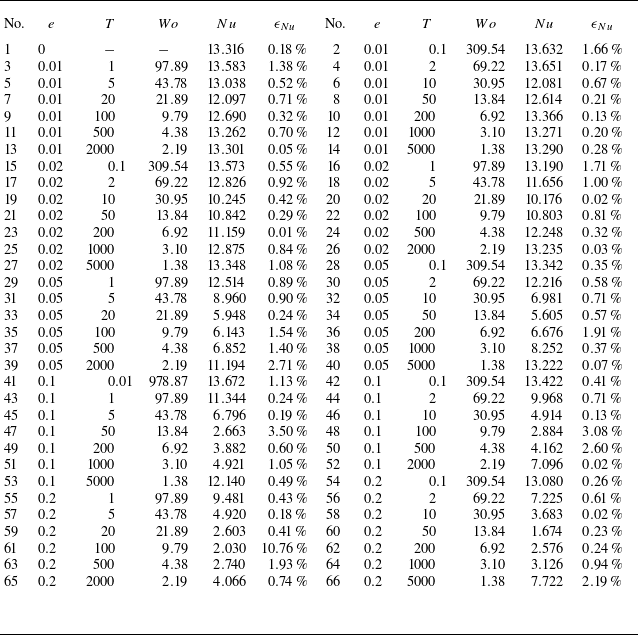
The parameter settings and the main results of the simulations considered in this work are listed in the table 2. The columns from left to right indicate the relative angular velocity amplitude
 $e$
, oscillation period
 $T$
, Womersley number
 $Wo$
, Nusselt number
 $Nu$
and its relative difference of two halves
 $\epsilon_{Nu}$
. Here,
 $Ra=10^7$
,
 $Pr=4.3$
,
 $Ro^{-1}=20$
and
 $\eta=0.5$
are fixed and the resolution
 $(N_r\times N_\varphi\times N_z)=(128\times1536\times2)$
is used for all the cases.
Simulation parameters. The columns from left to right indicate the relative angular velocity amplitude
 $e$
, oscillation period
 $T$
, Womersley number
 $Wo$
, Nusselt number
 $Nu$
and its relative difference of two halves
 $\epsilon _{Nu}$
. Here,
 $Ra=10^7$
,
 $Pr=4.3$
,
 $Ro^{-1}=20$
and
 $\eta =0.5$
are fixed for the simulation cases. The resolution
 $(N_r\times N_\varphi \times N_z)=(128\times 1536\times 2)$
is used for all the cases.