

Heterogeneity of Preference: Nuisance or Substance?
It’s late in the evening and Mike has lost his driver’s license. He believes it fell out of his pocket while he was jogging on the trail that circles the parking lot. He returns to the parking lot and searches underneath the single bright street light at the center of the lot. But all he finds is litter. Mike looks under a light where it is easier to see objects on the ground. It is true that his average location during his jog around the lot would be roughly near the light, but it is a logical fallacy to predict that his permit must lie under the light if it fell out of his pocket during his jog. It is no surprise that he finds nothing of value.
This metaphor illustrates how deriving predictions at an aggregate level sometimes lacks a logical foundation and can be counter-productive. The metaphor also suggests that two errors do not make one right. Repeating leaps of scientific reasoning in replication may perpetuate unwarranted scientific conclusions. Just as Mike would be well advised to take his route into account when looking for his belongings, so might behavioral decision researchers benefit from considering scientific predictions that don’t contradict the diversity of preferences a theory or hypothesis permits. This diversity is genuinely part of the theory, rather than an error term that one might shrug off as a nuisance.
It is common in behavioral decision research, for example, in papers claiming that Cumulative Prospect Theory (CPT) cannot account for a finding, to reduce that entire theory down to a single preference pattern. For instance, as Regenwetter and Robinson (Reference Regenwetter and Robinson2017) have pointed out, papers often limit themselves to the single preference pattern associated with Tversky and Kahneman’s (Reference Tversky and Kahneman1992) median parameter estimates (for high-profile examples, see e.g. Birnbaum, Reference Birnbaum2008; Brandstätter, Gigerenzer, & Hertwig, Reference Brandstätter, Gigerenzer and Hertwig2006). Since these are medians of parameters defined on a continuous domain, there is no reason to expect that anyone satisfying CPT would actually have the preference pattern associated with these particular parameter values (see also Regenwetter & Robinson, Reference Regenwetter and Robinson2019; Robinson, Wang, & Regenwetter, Reference Robinson, Wang and Regenwetter2019). Comparing the pattern of modal choices or tallying the choices consistent with the single preference pattern associated with such aggregate-level “prior parameters” is akin to looking only under the bright light where it is easy to see objects on the ground, but where there is, a priori, nothing of value to find. Rejecting such a theory once, and then again in a replication that uses the same approach and the same incorrect line of reasoning, is like finding only litter under two parking lot lights. Just as Mike might find his lost driver’s license if he took the heterogeneity in his locations seriously, so can decision research gain tremendous traction by tracking heterogeneity of preference as a precious source of information instead of dismissing and discarding it as a nuisance. The literature has issued numerous warnings about this and related challenges (e.g., Blavatskyy & Pogrebna, Reference Blavatskyy and Pogrebna2010; Block & Marschak, Reference Block, Marschak, Olkin, Ghurye, Hoeffding, Madow and Mann1960; Harless & Camerer, Reference Harless and Camerer1994; Hey, Reference Hey2005; Hey & Orme, Reference Hey and Orme1994; Luce, Reference Luce1959, Reference Luce1995; Luce & Suppes, Reference Luce, Suppes, Luce, Bush and Galanter1965; Loomes & Sugden, Reference Loomes and Sugden1995; Regenwetter et al., Reference Regenwetter, Davis-Stober, Lim, Guo, Popova, Zwilling and Messner2014; Stott, Reference Stott2006; Wilcox, Reference Wilcox, Cox and Harrison2008). Building on four in-depth prior papers (Regenwetter et al., Reference Regenwetter, Davis-Stober, Lim, Guo, Popova, Zwilling and Messner2014; Regenwetter & Robinson, Reference Regenwetter and Robinson2017, Reference Regenwetter and Robinson2019; Robinson et al., Reference Robinson, Wang and Regenwetter2019), this tutorial details what one gains by tracking the heterogeneity of preferences that is inherent to the theory.
Illustrative Example
Throughout the tutorial, we revisit a study by Barron and Ursino (Reference Barron and Ursino2013) as an illustrative example. Barron and Ursino (Reference Barron and Ursino2013) studied the description-experience (DE) gap, according to which decision making behavior systematically differs under conditions in which people are explicitly provided with information regarding payoffs and their probabilities versus conditions by which they learn payoffs and their probabilities through an experiential process such as free-sampling or repeated choice from an urn. Some, but not all, researchers formally define the DE gap in terms of Cumulative Prospect Theory (henceforth CPT). In its standard form, CPT models decisions using a value function v and probability weighting functions w + and w − for gains and losses, with parameters α, β, γ, δ, λ, of the form
 $$v(x) = \left\{ {\matrix{ {{x^{\rm{\alpha }}}} \hfill & {if\,x \ge 0\, & \left( {with\,0 \le {\rm{\alpha }} \le 1} \right),} \hfill \cr { - {\rm{\lambda }}{{( - x)}^{\rm{\beta }}}} \hfill & {if\,x < 0\, & \left( {with\,0 \le {\rm{\beta }} \le 1;0 < {\rm{\lambda }}} \right),} \hfill \cr} } \right.$$
 $${w^ + }\left( p \right) = {{{p^\gamma }} \over {{{\left( {{p^\gamma } + {{(1 - p)}^\gamma }} \right)}^{{1 \over \gamma }}}}} & \left( {with\,0 \le {\rm{\gamma }} < 1} \right),$$
 $${w^ - }\left( p \right) = {{{p^\delta }} \over {{{\left( {{p^\delta } + {{(1 - p)}^\delta }} \right)}^{{1 \over {\rm{\delta }}}}}}} & \left( {with\,0 \le {\rm{\delta }} < 1} \right),$$
where x are monetary amounts and p are probabilities, and where γ, δ < 1 captures overweighting of small probabilities. It is common nowadays to consider a broader range for γ, δ and to report that experience-based paradigms yield behavior consistent with underweighting of small probabilities (γ, δ > 1), whereas description-based paradigms yield behavior consistent with overweighting of small probabilities (γ, δ < 1) in CPT (see, e.g. Hertwig & Erev, Reference Hertwig and Erev2009).
Some of the debate centers on whether the DE gap reflects a true difference between how people weigh prospects across the two conditions, or is an artifact of under-sampling of low probability events in experience-based groups (Fox & Hadar, Reference Fox and Hadar2006; Hadar & Fox, Reference Hadar and Fox2009). Barron and Ursino (Reference Barron and Ursino2013) examined this question by conducting two experiments in which they controlled for bias in sampling and by reanalyzing previous data from a repeated choice (experience) paradigm of Barron and Erev (Reference Barron and Erev2003). For the reanalysis, the authors focused on only those participants who had sampled the low probability event sufficiently often to observe the approximate underlying probability distribution (within a margin of error of ± 1 SD of the underlying probability). Based on these analyses, the authors reported that for 4 out of 6 pairs of decision problems, the percentage of choices did not differ statistically significantly from those observed in the original paper (Barron & Erev, Reference Barron and Erev2003). For the two remaining gambles, they reported a significant change in choice frequencies. As we discuss in more detail in Appendix A, we are unable to reproduce these findings: There are ambiguities regarding Barron and Ursino’s test statistic, and, more importantly their sample size. While they apparently used the number of participants as sample size, one could also take into account that each participant, in turn, generated numerous observations because they made numerous choices. Ignoring the latter gives hard-to-interpret choice proportions and may yield an underpowered test, whereas including it may violate iid assumptions presumed by the statistical test. In our analyses, we will consider both ways of tallying the sample size (and both caveats will apply with these data).
Barron and Ursino (Reference Barron and Ursino2013) reported that modal choices were ‘consistent’ with underweightingFootnote 1 and concluded (abstract) that the reanalysis “reveals that the gap persists even when subjects observe the expected frequency of rare events” and furthermore, that the “results of the two experiments strengthen the suggestion that descriptive theories of choice that assume overweighting of small probabilities are not useful in describing decisions from experience.” We start our discussion by showing first that Barron and Ursino (Reference Barron and Ursino2013) drew these latter conclusions without genuinely considering the heterogeneity of CPT’s predictions.
Predictions from Cumulative Prospect Theory
Recommendation 1:
Before running a study aimed at comparing two or more decision theories, it is useful to inspect the domain of permissible preference states under each theory and to understand how much the theories overlap in the preference patterns they allow. That is, it is useful to assess how easily the theories can mimic each other on the stimulus set under consideration. Reducing, instead, each theory to one single preference pattern as a proxy for that theory, can jeopardize the interpretability of the entire study.
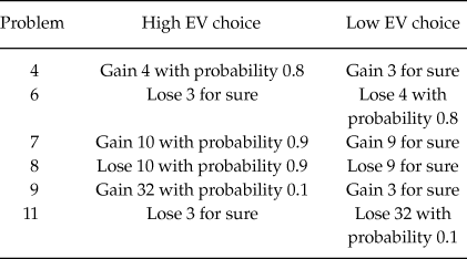
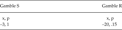
For our illustrations, we concentrate on the second half of Barron and Ursino (Reference Barron and Ursino2013). In their reanalysis of the data from Barron and Erev (Reference Barron and Erev2003), they used six decision problems reported also in their Table 5 (see our Table 1). In their own Experiment 2, “participants chose between two unmarked buttons presented on the screen. Each button was associated with one of two distributions referred to here as S (for safe) and R (for risky). The S distribution provided a certain loss of 3 points while the R distribution provided a loss of 20 points with probability 0.15 and zero otherwise” (Baron and Ursino, Reference Barron and Ursino2013, p. 284). We show these also in Table C1 of Appendix C.
Decision Problems of Barron & Erev (Reference Barron and Erev2003) used in the Reanalysis by Barron & Ursino (Reference Barron and Ursino2013) Adapted from their Table 5

We start by considering the heterogeneous preferences predicted by CPT for the six stimuli in Table 1. We distinguish two cases: CPT with overweighting of small probabilities (γ, δ < 1) and CPT with underweighting of small probabilities (γ, δ > 1). In an ideal situation, the scholar would determine all possible preference patterns that are permitted by a theory. Following a path of least resistance, we first ran a discrete grid search that considered a large number of parameter combinations in Equations 1–3. We considered a trillion combined parameter values for overweighting and a trillion combined parameter values for underweighting in CPT. Specifically, for α, β, we considered values from .001 to 1.0, using a step size of .001. For δ and γ and overweighting, we considered values from .001 to .999, using a step size of .001. Similarly, for underweighting, we used values for δ and γ with that same step size from 1.001 to 2. Since no decision problems involved both gains and losses, we considered gains and losses independently, fixing λ to 1, with no loss in generality.
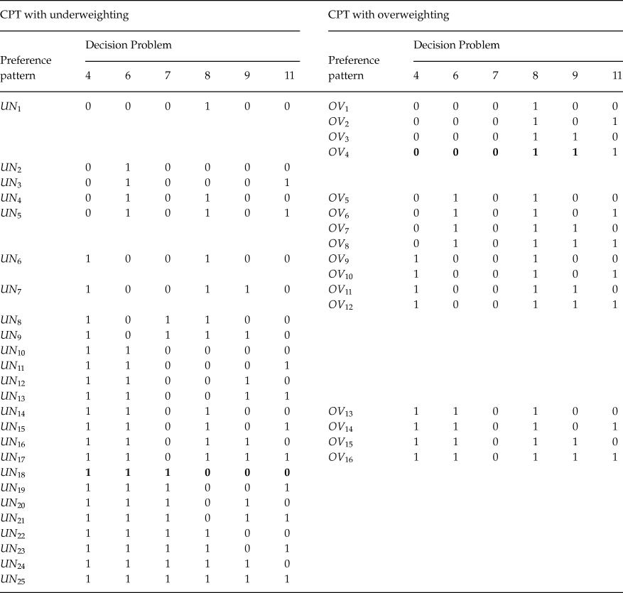
Disregarding, for a moment, indifference (which none of the parameter values in our grid search produced), there are 26 = 64 distinct possible preference patterns for six decision problems. Of these, our grid search for CPT with overweighting of small probabilities generated 16, as marked by OV 1 − OV 16 in the right side of Table 2. On the other hand, the grid search for CPT with underweighting of small probabilities generated 25 different patterns, as marked by UN 1 − UN 25 in the table. Nine of these preference patterns are consistent with both over- and underweighting of small probabilities.
Preference Patterns according to CPT with Underweighting (UN) and Overweighting (OV)

Note: A “1” entry denotes a preference for option H (high expected value), a “0” entry denotes a preference for option L (low expected value). The Decision Problem labels are taken from Barron and Ursino (Reference Barron and Ursino2013). The boldface pattern UN 18 appears to be their proxy for underweighting. The boldfaced pattern OV 4, which can be derived from the median parameter estimates of Tversky and Kahneman (Reference Tversky and Kahneman1992), is their declared proxy for CPT with overweighting.
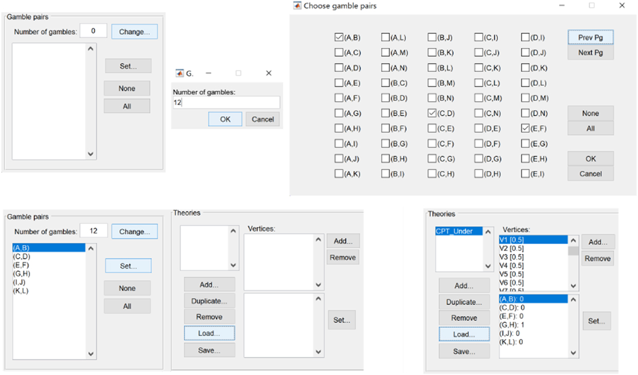
This heavy overlap threatens one’s ability to diagnose whether decision makers over- or underweight small probabilities, especially if we treat heterogeneity of behavior as a nuisance. This is because, in the latter case, there are nine scenarios of a potential shared preference pattern in which these stimuli do not differentiate between over- and underweighting. In this tutorial, we rely on the QTest open-source public-domain softwareFootnote 2 to illustrate a complete quantitative analysis. Figure 1 gives some milestone screenshots of portions of the graphical user interface (GUI) from the process of loading the preference patterns OV 1 − OV 16 and UN 1 − UN 25 into QTest. Appendix B provides screenshots of the input files.
Loading predicted preference patterns into QTest: In the “Gamble pairs” section of the GUI press “Change...” and set the “Number of gambles” to 12, then select “Set” and choose 12 distinct pairs of labels. In the “Theories” section click on “Load...” and direct the software to the file containing all preference patterns (see Figure B1 in Appendix B). The last screenshot shows the “Theories” section of the interface after “CPT_Under” has been loaded.

Returning to the possibility of indifference, the parameters underlying CPT form a continuum that we approximated with a discrete grid search. Consider, for example, OV 1 and OV 2, which differ only in the preference for Decision Problem 11. In some of the models that follow, we implicitly also include the preference pattern that results from replacing the preference in Decision Problem 11 in OV 1 and OV 2 by a pairwise indifference. From the point of view of CPT, these are knife-edge situations in which Equations 1–3 must generate exactly equal overall utilities for the two choice options in Decision Problem 11.
Having applied Recommendation 1 to the six decision problems of Table 2, we now apply it to the single gamble pair in Experiment 2 of Barron and Ursino (Reference Barron and Ursino2013). In Appendix C, we show that CPT with underweighting of small probabilities predicts that the decision maker prefers gamble R to gamble S regardless of parameter values. For CPT with overweighting of small probabilities, on the other hand, depending on the parameter values, the decision maker can either prefer R to S (e.g., with δ = .69, β = .88, Tversky and Kahneman’s median parameter estimates) or prefer S to R (e.g., with δ = .69, β = .8). In a nutshell: Barron and Ursino’s R/S stimulus pair is problematic for diagnosing over- versus underweighting, because CPT with overweighting of small probabilities can perfectly mimic CPT with underweighting.
Nuisance Model versus Substance Model
Recommendation 2:
It is useful, for any given core theory, such as CPT, to distinguish different types of heterogeneity:
1. Treating heterogeneity of behavior in a population as a nuisance means assuming a single shared (i.e., unanimous) deterministic preference. This is extremely restrictive. We find it very implausible, but, like Barron and Ursino (Reference Barron and Ursino2013), many papers use methods that are difficult to interpret short of making that assumption.
2. While different people may have different preferences consistent with the same core theory, individual preferences may be deterministic.
3. Individual preferences may be uncertain and different people may satisfy the same or different probability distributions over permissible preference states.
4. In all of the above scenarios, responses may or may not be error prone.
There are many different possible models to capture these scenarios. Different models often generate profoundly different predictions about behavior (see, e.g., Marley & Regenwetter, Reference Marley, Regenwetter, Batchelder, Colonius, Dzhafarov and Myung2017; Regenwetter et al., Reference Regenwetter, Davis-Stober, Lim, Guo, Popova, Zwilling and Messner2014; Regenwetter & Robinson, Reference Regenwetter and Robinson2017, for introductions, surveys, and guides). Here, we consider two types of models. We use simple names that reflect that one model class treats heterogeneity as a nuisance, whereas the other treats it as substance.
According to the “Nuisance Model” participants share a single (deterministic but unspecified) preference pattern and any deviations from this shared preference is due to probabilistic response error. Formally, writing P xy to denote the probability that x is chosen over y, according to the Nuisance Model
 $${P_{xy}} \ge 1 - {\rm{\tau }} &amp; if\,and\,only\,if\,x\,is\,unanimously\,preferred\,to\,y.$$
According to the “Substance Model,” the source of heterogeneity in observed choice behavior is uncertainty in decision-makers’ preference states, genuine individual differences, compounded with potential errors in responses. In an effort to keep the model parsimonious, we only allow for errors in responses when a “random preference” model, regardless of the distribution over heterogeneous preference states, assigns a pairwise preference probability of one or zero.Footnote 3 Formally, writing  $P\left( \succ \right)$ for the probability of preference pattern
 $\succ and\,x \succ y$ to denote that x is preferred to y in preference state
 $\succ$, let
 $${R_{xy}} = \sum\nolimits_{all\, \succ \,in\,CPT\,with\,x\, \succ \,y} {P\left( \succ \right)} . &amp; \left( {Random\,Preference\,Model} \right)$$
According to the Substance Model
 $${P_{xy}}\left\{ {\matrix{ { = {R_{xy}}} \hfill &amp; {if\,there\,exists\,a\,distribution\,P\,with\,0 \ne {R_{xy}} \ne 1,} \hfill \cr { \le .25} \hfill &amp; {if\,0 = {R_{xy}}\,for\,every\,distribution\,P,} \hfill \cr { \ge .75} \hfill &amp; {if\,{R_{xy}} = 1\,for\,every\,distribution\,P.} \hfill \cr} } \right.$$
In the terminology of Regenwetter and Robinson (Reference Regenwetter and Robinson2017) this is a type of “hybrid model” that incorporates components of a random preference model (5) and an error model (4). The choice of an upper bound on error rates is up to the scholar. Here, since this is an illustration for a tutorial, we consider a single model with an upper bound of 25% on error rates. That design choice is partially inspired by Harless and Camerer’s (Reference Harless and Camerer1994) recommendation of 25% errors in probabilistic error models for preferential choice. In contrast to them, however, we use 25% as an upper bound rather than a point hypothesis about error rates.
For CPT with overweighting of small probabilities, respectively CPT with underweighting of small probabilities, we consider all conceivable probability distributions over the 16 preference states OV 1 − OV 16, respectively all distributions over UN 1 − UN 25. As we discuss in Appendix D, a random preference model for CPT with overweighting leads to deterministic choice for Decision Problems 7 & 8, hence in this case, the Substance Model (6) augments the random preference model by allowing up to 25% error on those decision problems. As we also show in the next section, a random preference model for CPT with underweighting does not imply deterministic choice, hence the Substance Model for CPT with underweighting is the same as the random preference model for that case, and, for the sake of parsimony, it does not include an error term.
The Nuisance Model (unanimous preference, error-prone responses) and the Substance Model (probabilistic preferences, error-prone responses only where the random preference model predicts deterministic choice) are two parsimonious simple examples of a panoply of possible approaches.
Predictions
Nuisance Model: The predicted choice probabilities according to the Nuisance Model are directly given in its definition (4) above. It is worth noting that this model is not mathematically as simplistic as it appears at first sight. This is because, as we would argue to be the case here, the unanimous preference state is normally unknown. Hence, it must be treated as a free parameter in statistical inference. Furthermore, the model is characterized by one or multiple systems of inequality constraints on probabilities. That makes it an “order-constrained model,” which requires advanced statistical methods (see, e.g., Davis-Stober, Reference Davis-Stober2009; Klugkist & Hoijtink, Reference Klugkist and Hoijtink2007; Myung, Karabatsos, & Iverson, Reference Myung, Karabatsos and Iverson2005; Regenwetter et al., Reference Regenwetter, Davis-Stober, Lim, Guo, Popova, Zwilling and Messner2014). We provide the main steps for reproducing our analysis using the QTest software that is designed for such inference.
If we either hypothesize or assume that the population (unanimously) has the single shared deterministic preference pattern UN 18, then the Nuisance Model, with an upper bound  ${\rm{\tau }} = {1 \over 2}$ on error probabilities, implies that (up to sampling variability in the sample of respondents) the modal respondent chooses H in Decision Problems 4, 6, 7 and chooses L in Decision Problems 8, 9, and 11. This is the pattern of empirical modal choices that Barron and Ursino (Reference Barron and Ursino2013) observe in both the original Barron and Erev (Reference Barron and Erev2003) data and in their own subset of those data (see also the “perfect fit” of the Nuisance Model for underweighting discussed later). Even though CPT with over- and underweighting share many preference patterns, none of the 16 possible preference patterns for CPT with overweighting, that we found in our grid search, predict that same pattern UN 18. At the same time, however, there are 24 other patterns that CPT with underweighting permits. The Nuisance Model for CPT with underweighting encompasses 25 different patterns of modal choice. Hence, the full-fledged Nuisance Model of CPT with underweighting forms a rather complicated collection of sets of constraints on binary choice probabilities (mathematically, it forms a disjoint union of 25 distinct hypercubes of side length 1 − τ ); and CPT with overweighting likewise forms a rather complicated collection of sets of constraints on binary choice probabilities (mathematically, it forms a disjoint union of 16 distinct hypercubes of length 1 − τ, altogether 9 of which are shared with the other model.)
Substance Model: Figuring out the permissible choice probabilities according to the random preference model and, hence, the Substance Model, involves some mathematical work. While we give some specifics, we omit most of the details here (see, e.g., Guo & Regenwetter, Reference Guo and Regenwetter2014; Regenwetter & Cavagnaro, Reference Regenwetter and Cavagnaro2019; Regenwetter, Dana, & Davis-Stober, Reference Regenwetter, Dana and Davis-Stober2011; Regenwetter & Davis-Stober, Reference Regenwetter and Davis-Stober2012; Regenwetter et al., Reference Regenwetter, Davis-Stober, Lim, Guo, Popova, Zwilling and Messner2014; Regenwetter & Robinson, Reference Regenwetter and Robinson2017; Zwilling et al., Reference Zwilling, Cavagnaro, Regenwetter, Lim, Fields and Zhang2019, for detailed examples, related tutorials, and other useful pointers).
Let P HL(i) denote the probability of choosing H rather than L in Decision Problem i. For CPT with underweighting and for these decision problems, binary choice probabilities satisfy the random preference model (and hence the Substance Model, since no choice probabilities are forced to be zero or one) if and only if
 $$\left( {1 - {P_{HL}}\left( 8 \right)} \right) = {P_{LH}}\left( 8 \right) \le {P_{HL}}\left( 6 \right),$$
 $$max\left( {{P_{HL}}\left( 7 \right),{P_{HL}}\left( 9 \right)} \right) \le {P_{HL}}\left( 4 \right)\,\,\,and$$
 $${P_{HL}}\left( {11} \right) \le {P_{HL}}\left( 6 \right).$$
The necessity of these conditions becomes apparent from noticing that, no matter which UN preference pattern one considers, whenever L is preferred in Decision Problem 8, then H is preferred in Decision Problem 6, but the converse does not hold. Similarly, no matter which UN preference pattern, whenever H is preferred in Decision Problem 7, then H is also preferred in Decision Problem 4, but not vice versa. Likewise, whenever H is preferred in Decision Problem 9, then H is also preferred in Decision Problem 4, but not vice versa. No matter which UN preference pattern, whenever H is preferred in Decision Problem 11, then H is also preferred in Decision Problem 6, but the converse does not hold. Those observations imply that, regardless of the probability distribution over preference states, the above inequality constraints have to hold. Plugging in all possible ways of satisfying these constraints with probabilities zero or one gives back all the permissible preference patterns. This proves the sufficiency of the constraints (7)–(9) to completely characterize the parameter space of the model.
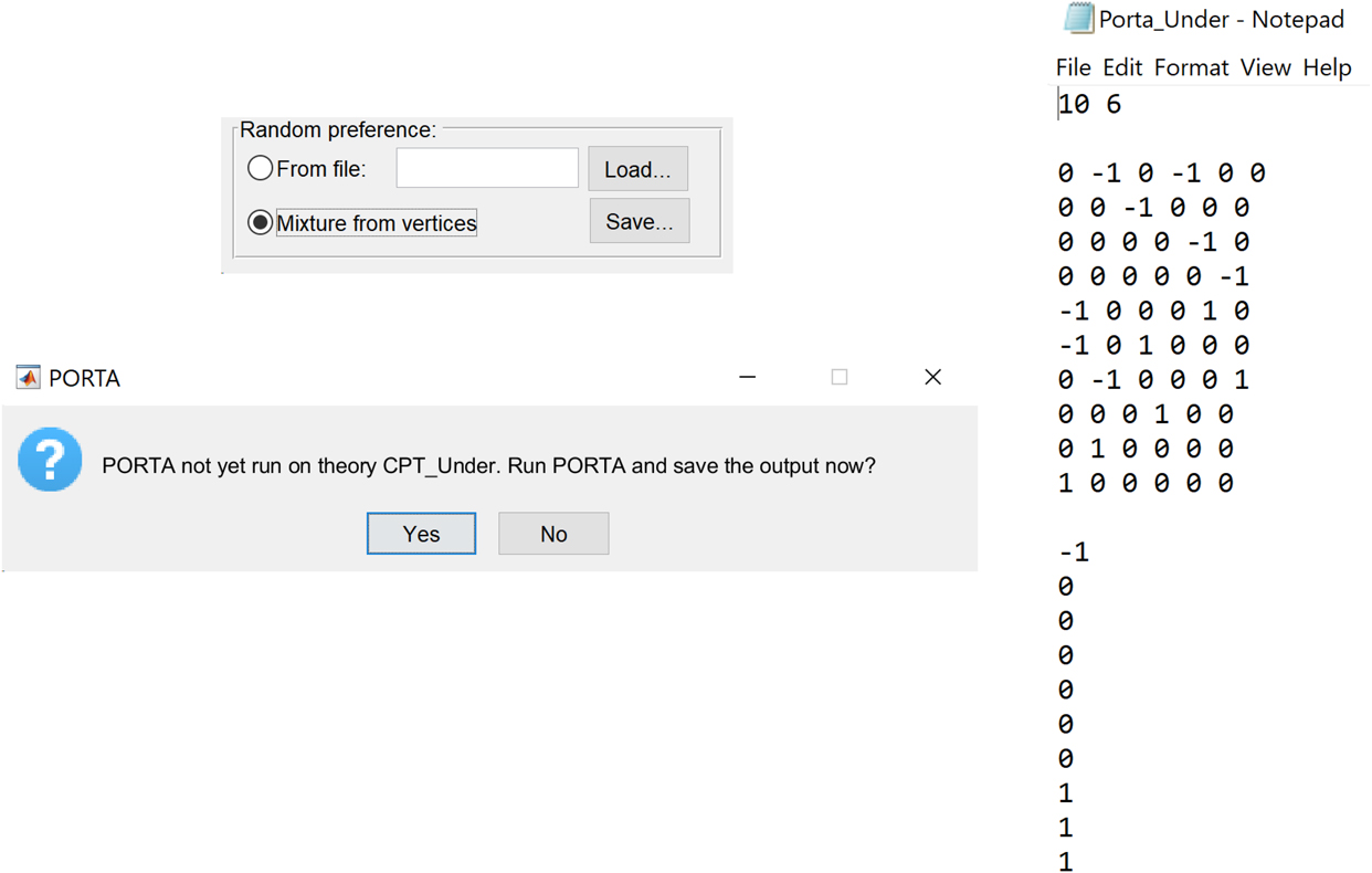
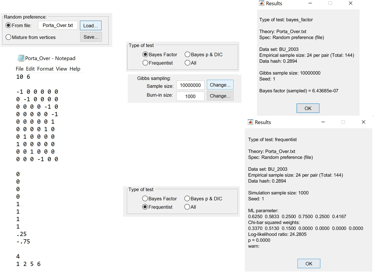
Figure 2 shows how one can derive these constraints by calling the public domain software Porta from QTest. For example, running Porta for the 25 preference patterns of CPT_Under generates a text file like the one partially shown in the right-most screenshot of Figure 2. The first line of the file states that there are 10 inequalities in six variables. The first two lines of the matrix below, together with the first two entries in the column vector at the bottom of the screenshot mean that, with the labels used in QTest,
 $$\matrix{ {0 \times {P_{AB}} - 1 \times {P_{CD}} + 0 \times {P_{EF}} - 1 \times {P_{GH}} + 0 \times {P_{IJ}} \le - 1,} \cr {0 \times {P_{AB}} + 0 \times {P_{CD}} - 1 \times {P_{EF}} + 0 \times {P_{GH}} + 0 \times {P_{IJ}} \le 0,} \cr}$$
i.e., dropping terms that are multiplied by zero, and using our labels here,
 $$\matrix{ { - {P_{HL}}\left( 6 \right) - {P_{HL}}\left( 8 \right) \le - 1,} \cr { - {P_{HL}}\left( 7 \right) \le 0.} \cr}$$
Calling PORTA to characterize the random preference model: In the “Random preference” section of the GUI, select “Mixture from vertices” then click “Save...” and QTest will generate a popup window like the one shown in the lower left screenshot. Completion of this process will generate a text file, part of which is shown in the screenshot on the right.

This gives Inequality 7 as well as one of the conditions that binary choice probabilities must be in the interval [0, 1]:
 $$\matrix{ {1 - {P_{HL}}\left( 8 \right) \le {P_{HL}}\left( 6 \right),} \cr {0 \le {P_{HL}}\left( 7 \right).} \cr}$$
The rest of the Porta output file likewise states an additional eight nonredundant inequality constraints on binary choice probabilities.
We now proceed to overweighting. We show that the stimuli in this study are such that a model of CPT with overweighting that allows for heterogeneity of preferences is extremely restrictive on two stimuli, but vacuous on the other four. Table 2 reveals that, no matter which of preference states OV 1 − OV 16 we consider, CPT with overweighting of small probabilities predicts that one prefers L in Decision Problem 7 and H in Decision Problem 8. Therefore, if our grid search found all (strict) preference patterns for these two decision problems, then a random preference model of CPT with overweighting predicts P HL = 0 in Decision Problem 7 and P HL = 1 in Decision Problem 8. In Appendix D we directly prove these two predictions without reliance on a grid search.
Consequently, in the Substance Model, we permit for response error with probability up to .25 in Decision Problems 7 and 8. At the same time, if we concentrate only on Decision Problems 4, 6, 9, and 11, of the 24 = 16 preference patterns conceivable, every single one can be derived from CPT with overweighting with a suitable choice of parameters in CPT. Hence, if a given person satisfying CPT with overweighting is allowed to fluctuate in his or her preference state, or if different individuals satisfying CPT with overweighting are allowed to differ in their preference states, then Decision Problems 4, 6, 9, and 11 do not predict any constraints on choice probabilities according to either a random preference or the Substance Model. In all, the Substance Model for CPT with overweighting places no constraints on four of the six binary choice probabilities and places moderate constraints (error rates ≤ .25) on the remaining two choice probabilities:
 $$0 \le {P_{HL}}\left( 7 \right) \le .25;\,\,\,\,.75 \le {P_{HL}}\left( 8 \right) \le 1;\,\,\,\,0 \le {P_{HL}}\left( 4 \right),{P_{HL}}\left( 6 \right),{P_{HL}}\left( 9 \right),{P_{HL}}\left( {11} \right) \le 1.$$
Put simply, four of these Decision Problems are uninformative for evaluating CPT with overweighting in the presence of heterogeneity, whereas the other two Decision Problems are extraordinarily diagnostic.
Insufficiently frequently asked questions (iFAQ)
Regenwetter and Robinson (Reference Regenwetter and Robinson2017) have shown several reasoning fallacies that permeate behavioral decision research (see also Regenwetter & Robinson, Reference Regenwetter and Robinson2019). We first tackle their “Fallacy of Modal Choice.”
QUESTION 1.0: If most decision makers satisfy Theory X, then can we predict that the pattern of modal choices will satisfy Theory X, i.e., that ‘the modal decision maker satisfies X?’ In general, this conclusion is invalid. Short of adding very strong additional features to the premise, e.g. that there exists a majority of decision makers who share a single unanimous preference pattern, there is no logical merit to such an inference. We zoom into a specific example for illustration.
QUESTION 1.1 (CPT, with Decision Problems 4, 6, 7, 8, 9, 11): If most decision makers underweight small probabilities, then can we predict that the pattern of modal choices will be UN 18? The answer is no.
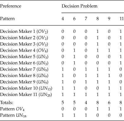
Consider the 11 hypothetical decision makers described in Table 3. To keep matters simple, suppose that they each have a single deterministic preference and that they make no errors in responses. Suppose that four of these decision-makers overweight small probabilities and that their preference patterns are OV 2, OV 2, OV 2 and OV 8, respectively. Suppose that the remaining seven participants, a substantial majority among 11 people, underweight small probabilities, and that their preference patterns are UN 3, UN 3, UN 9, UN 9, UN 9, UN 13 and UN 25, respectively. For such a combination of preferences, the predicted proportions of H choices , for Decision Problems 4, 6, 7, 8, 9, 11, are  ${5 \over {11}},{5 \over {11}},{4 \over {11}},{8 \over {11}},{6 \over {11}},{8 \over {11}}$, respectively. In Decision Problems 4, 6, 7, most people choose L, whereas in Decision Problems 8, 9, 11, most people choose H. This means that the predicted pattern of modal choices, or what is often misleadingly referred to as “the modal decision maker’s choice pattern,” is OV 4, and not a pattern permitted by underweighting. Even though the majority of participants underweight rare events, the pattern of predicted modal choices is a pattern consistent only with overweighting. Furthermore, this pattern is exactly the opposite of UN 18, which Barron and Ursino (Reference Barron and Ursino2013) use as a proxy for underweighting of small probabilities. It even happens to be the pattern predicted by CPT (with overweighting) with median parameter values of Tversky and Kahneman (Reference Tversky and Kahneman1992).
Hypothetical Preference Patterns of 11 Decision Makers, a Majority of whom Underweight Small Probabilities, and whose Pattern of Modal Choices is OV4. That Pattern is the Opposite of UN18 and Incompatible with all 25 Patterns We Found for Underweighting

We now turn to the “Fallacy of Choice Tallies” that Regenwetter and Robinson (Reference Regenwetter and Robinson2017) also showed to be very prevalent in the behavioral choice literature.
QUESTION 2.0: If all or most decision makers satisfy Theory X, then can we pick one of the preference patterns derived from Theory X and predict that the tally of choices consistent with that pattern, aggregated over trials, stimuli and participants will exceed  ${1 \over 2}$ of all observations? In general, this conclusion is invalid. Short of adding very strong additional features to the premise, e.g. that there exists a majority of decision makers who share a single unanimous preference pattern, there is no logical merit to such an inference. We zoom into a specific example for illustration.
QUESTION 2.1 (CPT, with Decision Problems 4, 6, 7, 8, 9, 11): If all or most decision makers underweight small probabilities, then will the tally of choices consistent with UN 18, aggregated over trials, stimuli and participants, automatically exceed  ${1 \over 2}$ of all observations? The answer is no.
QUESTION 2.2 (CPT, with Decision Problems 4, 6, 7, 8, 9, 11): The preference associated with the median parameter estimates of Tversky and Kahneman (1992) is OV 4. Therefore, if all or most decision makers overweight small probabilities, can we predict that the tally of choices consistent with OV 4, aggregated over trials, stimuli and participants, will exceed  ${1 \over 2}$ of all observations? The answer is no.
Let u i, respectively o j, denote the probability that a randomly sampled person, on a randomly sampled trial, has preference UN i, respectively OV j. Suppose that every person at every trial has one of these preference states, that is, suppose that  $\sum\nolimits_i^{25} {{u_i}} + \sum\nolimits_j^{16} {{o_j}} = 1$ and, for simplicity, suppose that nobody makes errors. Then, what is the expected proportion of choices consistent with UN 18, the pattern that Barron and Ursino (Reference Barron and Ursino2013) use as proxy for underweighting? For example, suppose that
 ${u_1} = {1 \over 4},{o_3} = {3 \over 4}.$ Since UN 1 matches UN 18 only for 2 of the six problems and since OV 3 matches UV 18 on one of the six problems, altogether
 ${u_1}{2 \over 6} + {o_3}{1 \over 6} = {1 \over 4} \times {2 \over 6} + {3 \over 4} \times {1 \over 6} = {5 \over {24}}$ of all choices will be consistent with UV 18. In general, the expected proportion of choices consistent with UN 18 is
 $$\matrix{ {{{2{{\bf{u}}_1} + 4{u_2} + 3{u_3} + 3{u_4} + 2{u_5} + 3{u_6} + 2{u_7} + 4{u_8} + 3{u_9} + 5{u_{10}}} \over 6}} \cr { + {{4{u_{11}} + 4{u_{12}} + 3{u_{13}} + 4{u_{14}} + 3{u_{15}} + 3{u_{16}} + 2{u_{17}} + 6{u_{18}} + 5{u_{19}} + 5{u_{20}}} \over 6}} \cr { + {{4{u_{21}} + 5{u_{22}} + 4{u_{23}} + 4{u_{24}} + 3{u_{25}}} \over 6}} \cr { + {{2{o_1} + {o_2} + {{\bf{o}}_3} + 3{o_5} + 2{o_6} + 2{o_7} + {o_8} + 3{o_9} + 2{o_{10}}} \over 6}} \cr { + {{2{o_{11}} + {o_{12}} + 4{o_{13}} + 3{o_{14}} + 3{o_{15}} + 2{o_{16}}} \over 6},} \cr}$$
where the boldfaced terms are those of the example. If all decision makers underweight small probabilities, i.e.,  $\sum\nolimits_i^{25} {{u_i}} = 1$ and all o j = 0, assuming error-free responses, then this expected proportion can take any value between
 ${1 \over 3}$ and 1. Permitting errors in responses broadens that range further. We see no reason to predict that this expected proportion will exceed
 ${1 \over 2}$. If most decision makers underweight small probabilities, i.e.,
 $\sum\nolimits_i^{25} {{u_i}} &gt; {1 \over 2}\,and\,\sum\nolimits_i^{16} {{o_j}} &lt; {1 \over 2}$, assuming error-free responses, then this proportion can take any value exceeding
 ${1 \over 6}$. Allowing errors in responses broadens that range further. Here again, we see no reason to predict that this expected proportion will exceed
 ${1 \over 2}$.
The expected proportion of choices consistent with OV 4 is
 $$\matrix{ {{{4{u_1} + 2{u_2} + 3{u_3} + 3{u_4} + 4{u_5} + 3{u_6} + 4{u_7} + 2{u_8} + 3{u_9} + {u_{10}}} \over 6}} \cr { + {{2{u_{11}} + 2{u_{12}} + 3{u_{13}} + 2{u_{14}} + 3{u_{15}} + 3{u_{16}} + 4{u_{17}} + {u_{19}} + {u_{20}}} \over 6}} \cr { + {{2{u_{21}} + {u_{22}} + 2{u_{23}} + 2{u_{24}} + 3{u_{25}}} \over 6}} \cr { + {{4{o_1} + 5{o_2} + 5{o_3} + 6{o_4} + 3{o_5} + 4{o_6} + 4{o_7} + 5{o_8} + 3{o_9} + 4{o_{10}}} \over 6}} \cr { + {{4{o_{11}} + 5{o_{12}} + 2{o_{13}} + 3{o_{14}} + 3{o_{15}} + 4{o_{16}}} \over 6}.} \cr}$$
If all decision makers overweight small probabilities, i.e.,  $\sum\nolimits_i^{16} {{o_j}} = 1$ and all u i = 0, assuming error-free responses, then this expected proportion can take any value between
 ${1 \over 3}$ and 1. Allowing errors in responses broadens that range further. We see no reason to predict that this expected proportion will exceed
 ${1 \over 2}$. If most decision makers overweight small probabilities, i.e.,
 $\sum\nolimits_i^{25} {{u_i}} &lt; {1 \over 2}\,and\,\sum\nolimits_i^{16} {{o_j}} &gt; {1 \over 2}$, assuming error-free responses, then this proportion can take any value exceeding
 ${1 \over 6}$. Allowing errors in responses broadens that range further. Once more, we see no reason to predict that this expected proportion will exceed
 ${1 \over 2}$.
In Barron and Ursino’s Experiment 2, since CPT with underweighting only permits preference of R over S, if all decision makers underweight small probabilities, then, (i) with error free choice, all choices must be R choices and (ii) with error prone choice we expect the proportion of R choices to be 1 - s, where s is the error rate. Since CPT with overweighting (considering a range of parameter values) permits either option to be preferred, regardless of whether we allow or disallow error, the expected proportion of S choices is not in any way constrained. This means that Table 6 of Barron and Ursino (Reference Barron and Ursino2013) which reports that, “consistent with underweighting,” the proportion of R choices is significantly greater than 0.5, is uninformative because that finding is equally consistent with either under- or overweighting. Testing whether the proportions significantly exceed  ${1 \over 2}$ is not based in testing CPT with over- or underweighting in the presence of heterogeneity of preferences. Barron and Ursino (Reference Barron and Ursino2013) did not spell out their rationale for carrying out these tests.
Findings
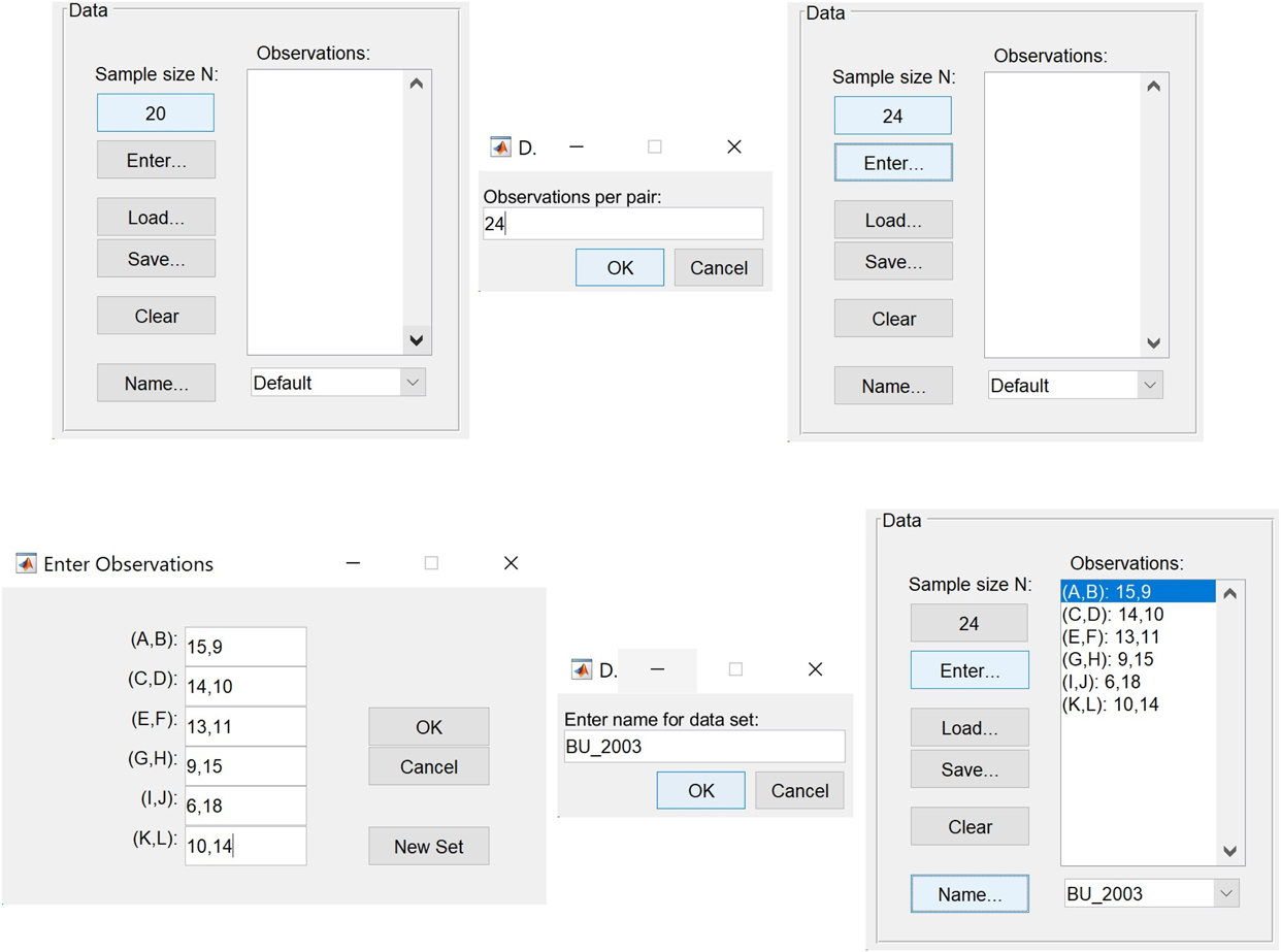
The second author, for a graduate student project on assessing the scientific merit of Barron and Ursino (Reference Barron and Ursino2013), carried out the mathematical analysis and the order-constrained statistical analysis using the public domain software QTest (Regenwetter et al., Reference Regenwetter, Davis-Stober, Lim, Guo, Popova, Zwilling and Messner2014; Zwilling et al., Reference Zwilling, Cavagnaro, Regenwetter, Lim, Fields and Zhang2019). Table A1 in Appendix A shows our reconstruction of the choice frequencies, based on Table 5 of Barron and Ursino (Reference Barron and Ursino2013). Figure 3 shows how to enter such data into QTest manually (where necessary, we rounded the frequencies to the nearest integers). Figures 4 – 6 show some key steps in running the analysis in QTest.
Loading the (rounded) data from Barron and Erev (Reference Barron and Erev2003) into QTest with an assumed sample size of 24: In the “Data” section of the GUI, click on the preset value “20” and enter “24” for the number of “Observations per pair.” Select “Enter” and type in the inferred frequencies (see Table A1 and the surrounding cautions in Appendix A) and give the dataset a name. The bottom right screenshot shows the “Data” section after the data entry for “BU_2003” is completed.

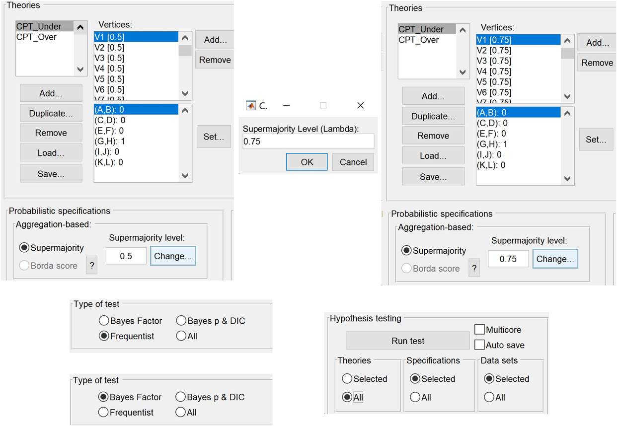
Order-constrained inference for the Nuisance Model in QTest: With the preference patterns loaded, the user selects “Supermajority” in the GUI section titled “Probabilistic Specifications” and “Aggregation-based” and sets the “Supermajority Level (Lambda)” to 1 - τ. In the “Type of Test” section of the GUI, the user chooses “Frequentist” or “Bayes Factor” and tells the program to “Run test” for “All” Theories in the “Hypothesis testing” section of the GUI.

Our findings are summarized in Table 4, with the top half assuming a large sample size of 9,600 choice per option pair, for the 2003 master data set, and the bottom half assuming a small sample size of 24 participants, for the 2003 master data set (see Table A1 for specifics). We rely on Bayes Factors (BF, see also Kass & Raftery, Reference Kass and Raftery1995) to quantify the evidence in favor or against a given model. For a formal statement of the likelihood function and a discussion of technical matters, including independence, stationarity, prior distribution, and exchangeability assumptions, as well as how they relate to common approaches in the literature, see the four detailed tutorial papers by Regenwetter et al. (Reference Regenwetter, Davis-Stober, Lim, Guo, Popova, Zwilling and Messner2014); Regenwetter and Davis-Stober (Reference Regenwetter and Davis-Stober2018); Regenwetter and Cavagnaro (Reference Regenwetter and Cavagnaro2019); Zwilling et al. (Reference Zwilling, Cavagnaro, Regenwetter, Lim, Fields and Zhang2019). We use the standard convention and terminology that a BF < 0.3 indicates “strong evidence against” and BF > 3.2 “strong evidence in favor” of a given model, with intermediate values offering “circumstantial evidence” (Jeffreys, Reference Jeffreys1961). We have boldfaced the first case, used a larger and underlined font for the second case, and placed the latter case into parenthesis for easy parsing. All Bayes Factors in Table 4 are in comparison to an unconstrained model. We also provide p values of frequentist hypothesis tests, treating each model as a null hypothesis in each case. Small p values are marked in boldface.
QTest Analysis of Barron & Erev’s (Reference Barron and Erev2003) Data that Barron & Ursino (Reference Barron and Ursino2013) Re-analyzed

The full data from Barron and Erev (Reference Barron and Erev2003) included many cases in which respondents experienced biased samples, and hence could not possibly know the ‘objective’ distributions underlying the lotteries. Short of reconstructing what each of them saw, it is not clear that modeling the full data with Cumulative Prospect Theory is even possible, since the theory needs probabilities as part of its input, and it would not make much sense to input hidden probabilities that respondents could not possibly know. Therefore, we start with the subsample of cases in which Barron and Ursino (Reference Barron and Ursino2013) considered the experience to be representative of the actual distribution. These analyses are marked 2013 in Table 4.
Nuisance Model: For large sample size, even when we permit very high error rates in responses (i.e., up to 50% when  ${\rm{\tau }} = {1 \over 2}$), the Bayesian analysis yields strong evidence against overweighting (BF < 10−100) and the frequentist hypothesis test is significant. However, with small sample size, the Bayesian evidence becomes circumstantial and the result of the frequentist hypothesis test becomes nonsignificant. For underweighting, restated in our terminology, as Barron and Ursino (Reference Barron and Ursino2013) reported, the pattern of modal choices fits preference pattern UN 18 of CPT with underweighting perfectly. Indeed, writing Q HL(i) to denote the proportion of H choices in Decision Problem i,
 $$\matrix{ {{Q_{HL}}\left( 1 \right) = 0.64 \ge {1 \over 2},\,\,\,\,{Q_{HL}}\left( 2 \right) = 0.56 \ge {1 \over 2},\,\,\,\,{Q_{HL}}\left( 3 \right) = 0.63 \ge {1 \over 2}} \cr {{Q_{HL}}\left( 4 \right) = 0.47 \le {1 \over 2},\,\,\,\,{Q_{HL}}\left( 5 \right) = 0.43 \le {1 \over 2},\,\,\,\,{Q_{HL}}\left( 6 \right) = 0.33 \le {1 \over 2}.} \cr}$$
This perfect fit of the Nuisance Model for CPT with underweighting and high error rates is also reflected in the p value of 1: No matter what significance level, we could not have sufficient evidence to reject the Null Hypothesis. A perfect fit in no way proves the Null Hypothesis to be true. Interestingly, the Bayesian analysis in Table 4 only yields circumstantial evidence in favor of underweighting with a BF = 2.56. While there is a perfect fit from a frequentist point of view, that modest Bayes Factor reflects the penalty for complexity because CPT with underweighting permits 25 different possible scenarios for the unanimous preference pattern. When the error rate is bounded at  ${\rm{\tau }} = {1 \over 4}$, we find strong evidence against CPT with both overweighting (BF < 10-100) and underweighting (BF < 10-100) and we find the frequentist test to yield rejections of the models.
Recall that there is some ambiguity as to how to treat sample size in the 2003 data set. Assuming 9,600 observations per binary choice may be problematic because those observations may not be exchangeableFootnote 4 and may not have arisen from a stationary distribution, hence raising questions about robustness in statistical inference. On the other hand, treating the data as originating from 24 observations implies nonsensical choice proportions in the original paper (see Appendix A) and jeopardizes statistical power. Unsurprisingly, as we compare the large sample and small sample analyses, with the exception of a perfect fit, evidence becomes less compelling. However, the results tell virtually the same story. The only place where a substantive conclusion is affected is in the frequentist analysis of the Nuisance Model with error rate  $\le {1 \over 2}$, which is rejected with large sample size, but not rejected with small sample size.
These results suggest that, with a unanimous preference and a high response error rate, these data may be more consistent with underweighting of rare events than overweighting. However, when allowing only a moderate error rate, we find strong evidence also against underweighting of rare events in decisions from experience. While we do not report the details in Table 4, we have also considered each single preference pattern as a possible unanimous preference, yielding 64 different nested submodels of the Nuisance Model with  ${\rm{\tau }} = {1 \over 4}$. By treating each of these 64 cases as a separate model on its own, we strongly boost each one for parsimony. Nonetheless, each of these models has a minuscule Bayes Factor (BF < 10-100). This gives very strong evidence against any unanimous preference pattern with moderate error rates. In other words, we have very strong evidence that, unless one permits a huge proportion of responses to be mistakes, heterogeneity is not a mere nuisance in these data. This result mirrors a similar finding of Regenwetter and Robinson (Reference Regenwetter and Robinson2017) on different data.
Substance Model : Our analysis yields strong evidence against the Substance Model of CPT with overweighting (BF < 10-100). For CPT with underweighting, substituting the choice proportions Q HL (i) for P HL (i) in Conditions 7–9, for the 2013 data, gives
 $$\matrix{ {{Q_{LH}}\left( 8 \right) = 0.53 \le 0.56 = {Q_{HL}}\left( 6 \right),} \cr {max\left( {{Q_{HL}}\left( 7 \right),{Q_{HL}}\left( 9 \right)} \right) = max\left( {0.63,0.43} \right) \le 0.64 = {P_{HL}}\left( 4 \right)\,\,\,\,and} \cr {{Q_{HL}}\left( {11} \right) = 0.33 \le 0.56 = {Q_{HL}}\left( 6 \right).} \cr}$$
Since the proportions satisfy the inequalities required of the probabilities, the best fitting probabilities are the same as the observed proportions. This explains the p value of 1 in the frequentist hypothesis tests of the random preference model of CPT with underweighting (hence the Substance Model), for the large sample size analysis. However, as we move to the small sample size analysis, where the reported proportions do not generate integer valued frequencies (see Table 5), rounding to integer valued frequencies leads to a small change in the effective proportions. This change is enough to violate one of the conditions above: Because, in this interpretation of the data, 13 people (out of 20) chose H over L in Problem 7 and 6 people (out of 10) did so in Problem 4, these numbers provide evidence against the prediction that P HL (7) ≤ P HL (4).
The Bayesian analysis provides strong evidence in favor (BF = 7.7) of the Substance Model for CPT with underweighting on the 2013 data, rewarding this model for its greater parsimony than the Nuisance Model with high response error rates. The Bayes Factor between the two models is  ${{7.7} \over {2.56}} = 3.01$. This means that, under the assumption that one or the other model holds, we have circumstantial evidence in favor of the Substance Model over the Nuisance Model with high permissible error rates. For the full data (marked 2003 in the lower panel of Table 4) that Barron and Ursino (Reference Barron and Ursino2013) took from Barron and Erev (Reference Barron and Erev2003), the results for the Nuisance Models and the result for the Substance Model of CPT with overweighting match those for the 2013 subsample. Interestingly, the Substance Model of CPT with underweighting of rare events does not fare well on the full 2003 data. The choice proportions violate Condition 7 and the analysis yields a small Bayes Factor (BF < 10−4), providing strong evidence against the model.
Comparing our results for the 2013 data with those of the 2003 data speaks to the discussion that motivated Barron and Ursino (Reference Barron and Ursino2013) to consider only participants who had experienced representative samples from the underlying distributions. Barron and Ursino (Reference Barron and Ursino2013) succeeded in extracting a subset of data for which CPT with underweighting provides an explanation of heterogeneous behavior. In Appendix A, we show that, when using the large sample size approach, the choice proportions for the 2013 data and the 2003 data are significantly different from each other. While some authors have questioned whether decision makers only appear to underweight objective probabilities when, in actuality they might overweight probabilities that are biased due to unrepresentative experienced samples, our reanalysis supports a diametrically opposite story in the case of a large sample size: In the 2003 data, which included experiences that Barron and Ursino (Reference Barron and Ursino2013) deemed as not representative of the objective probabilities in the decision problems, heterogeneous preferences with underweighting (through the lens of CPT using the objective, but in many cases hidden, probabilities) fail to account for the data, whereas, in the 2013 data, which concentrated on cases that Barron and Ursino (Reference Barron and Ursino2013) deemed representative of the underlying distributions, heterogeneous CPT with weighting parameters γ, δ > 1 accounts well for the data. However, for a small sample size interpretation of the data, none of the Bayes factors provide better than circumstantial evidence in favor of any of the models and some frequentist p values increase (except one case that we discussed earlier).
Discussion
This article is intended as a tutorial and as a blue-print for graduate student projects that aim to dig deeply into the merits of past work and that contemplate running replication studies of decision-making experiments.
Recommendations: We recommend that one should thoroughly scrutinize studies for their scientific merit before considering replication studies. For studies that suffer from unwarranted scientific reasoning, such as the Fallacy of Choice Tallies or the Fallacy of Modal Choice, it makes sense to replace, or at least augment, replications with improved methods. Secondly, we recommend that scholars should aim to understand the genuine heterogeneity of preferences permitted by each theory before attempting to let theories compete against each other. Understanding this heterogeneity is key towards designing diagnostic stimuli. Indiscriminately reducing a theory, like CPT or, say, a heuristic toolbox, to a single preference pattern as a proxy for the entire theory readily jeopardizes the interpretability of an entire study. Another recommendation gives an overview of different types of heterogeneity and cautions that, as discussed extensively in the literature, the many different models that formally capture these different sources of heterogeneity make profoundly different predictions about behavior.
Reassessing Barron and Ursino (2013) : We developed Nuisance Models and a Substance Model that formally derived predictions from explicitly stated assumptions, for Barron and Ursino’s stimuli that they borrowed from Barron and Erev (Reference Barron and Erev2003). We tested these models on the data that Barron and Ursino (Reference Barron and Ursino2013) extracted from Barron and Erev (Reference Barron and Erev2003) for their own re-analysis. The analysis with small assumed sample size leads to circumstantial evidence at best and strong evidence against some models at worst. The analysis using an assumed large sample size leads to more interesting findings, which we summarize next.
The analysis of the Nuisance Model with high response error rates provides strong evidence against overweighting and moderate evidence in favor of underweighting. However, when response error rates are limited to moderate levels, no model that treats heterogeneity of behavior as a nuisance, fares well at all.
The Substance Model provides strong evidence against CPT with overweighting under the assumption that response error rates are no higher than 25% for Decision Problems 7 and 8, where a random preference model would predict deterministic choice. This result is striking, given that four out of six stimuli are undiagnostic and the model places no constraints on the corresponding four choice probabilities. The Substance Model for CPT with underweighting, which is also a random preference model and which does not involve any response errors, provides a perfect fit for the 2013 data by frequentist standards and is supported with strong evidence through the lens of a Bayes Factor analysis. Strikingly, and in direct contrast with the literature that motivated Barron and Ursino’s study, the Substance Model for CPT with either over- or underweighting does not actually account well for the 2003 data. This ultimately strengthens Barron and Ursino’s core message about the high value of experience designs where the decision maker has, at least in principle, the opportunity to learn the underlying probability distribution. For those participants whose data are excluded in the 2013 data, we do not know the (biased) proportions of wins they experienced. In all, it is not particularly surprising if CPT with either over or underweighting of the objective probabilities fails to account for the full 2003 data. While we pointed out various major problems with Barron and Ursino’s approach, we support some of the conclusions they drew from re-analyzing the data of Barron and Erev (Reference Barron and Erev2003).
On the other hand, unfortunately, Barron and Ursino’s Experiment 2 used a pair of gambles that do not constrain the preference of a decision maker who satisfies CPT with overweighting. If they had observed 100% choices of R, this would have supported underweighting as the more parsimonious explanation for this stimulus set. But any other proportion of R choices creates an inherent ambiguity as to which is the better explanation for the data. Hence, we find that their Experiment 2 results are uninterpretable.
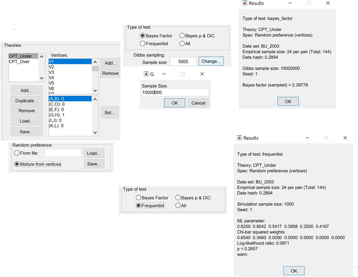
Quantitative Analysis of the Substance Model (Random Preference model) for Underweighting: Select the vertex description for CPT with underweighting, then in the “Random preference” section, select “Mixture from vertices” and select the desired test in the “Type of test” section of the GUI. For the Bayes factor, change the “Sample size” for “Gibbs Sampling” to a very large number before running the analysis. The right most screenshots show the QTest output for these analyses.

Quantitative Analysis of the Substance Model for Overweighting: In the “Random preference” section of the GUI, select “From File:” then navigate to the text file whose screenshot is shown on the lower left, and click “Load...” (see also Condition 10 in Section on Predictions). For the Bayes factor and the p value, proceed with the analysis in the same way as for the Substance Model for Underweighting.

Appendix A
Hypothesis tests in Table 5 of Barron & Ursino (Reference Barron and Ursino2013).
It is unclear what test Barron and Ursino (Reference Barron and Ursino2013) used in their Table 5. Writing p 1 and p 2 for two probabilities to be compared,  $\hat p_1 $ and
 $\hat p_2 $ for the observed proportions, Y 1 and Y 2 for the corresponding observed frequencies,
 $\hat p$ for the overall proportion, and n 1 and n 2 for the corresponding sample sizes, the standard hypothesis test for H 0 : p 1 = p 2 gives the z-score
 $$z = {{({{\hat{p}}_1} - {{\hat{p}}_2})} \over {\sqrt {\hat{p}(1 - \hat{p})\left( {{1 \over {{n_1}}} + {1 \over {{n_2}}}} \right)} }} &amp; where\,\hat{p} = {{{Y_1} + {Y_2}} \over {{n_1} + {n_2}}}.$$
Barron and Ursino (Reference Barron and Ursino2013) appear to use n 1 = 24 and n 2, according to Column 6 of their Table 5 (reproduced here as n 1 and n 2 in the upper half of our Table A1). They report that the proportions significantly differ in Problems 8 and 9 (p < .05), a finding that we cannot reproduce. We find all two-sided p values to exceed .34 when using the sample sizes in the top half of the table. That analysis leaves out that the observed proportions were, in actuality, calculated from thousands of observations. Hence, it may be severely underpowered. It is also unclear how, for example, the proportion of choices of H in Decision Problem 1 (in their Column 5, and our Column 6) could be 0.64 when the sample size is 10: No matter how many people out of N = 10 chose H, this proportion cannot equal 0.64, even with rounding. It does not make sense to treat that proportion as arising from 10 observations. (Notice also how our reconstructed choice frequencies Y 1 and Y 2 are nonintegers.) In our analyses of the probabilistic choice models, we rounded noninteger choice frequencies to the nearest integers.
Barron and Ursino (Reference Barron and Ursino2013) reported that the proportions in their table were “aggregated over subjects and over 400 trials” (p. 283). The lower half of our Table A1 shows the results for the same six hypothesis tests, assuming that the proportions are aggregated over 24 people and 400 trials in Column 4 of their Table 5 and aggregated over N people and 400 trials in their Column 5, with N given in their Column 6 (see our Table for the corresponding values of n 1 and n 2.).
Tests of Differences of Proportions based on Information from Table 5 of Barron and Ursino, Reference Barron and Ursino2013

With that assumption our reconstructed choice frequencies Y 1 and Y 2 are, indeed, integers. With these reconstructed data, we find all but one p value to be minuscule. A downside of this analysis is that the iid assumptions underlying this test may not hold. Regardless, we are unable to reproduce the results of Barron and Ursino (Reference Barron and Ursino2013), according to which the proportions significantly differ in Problems 8 and 9 at a 5% significance level. In the main text, we report analyses under both sets of reconstructed data given in Table A1.
Appendix B
Input Files for QTest
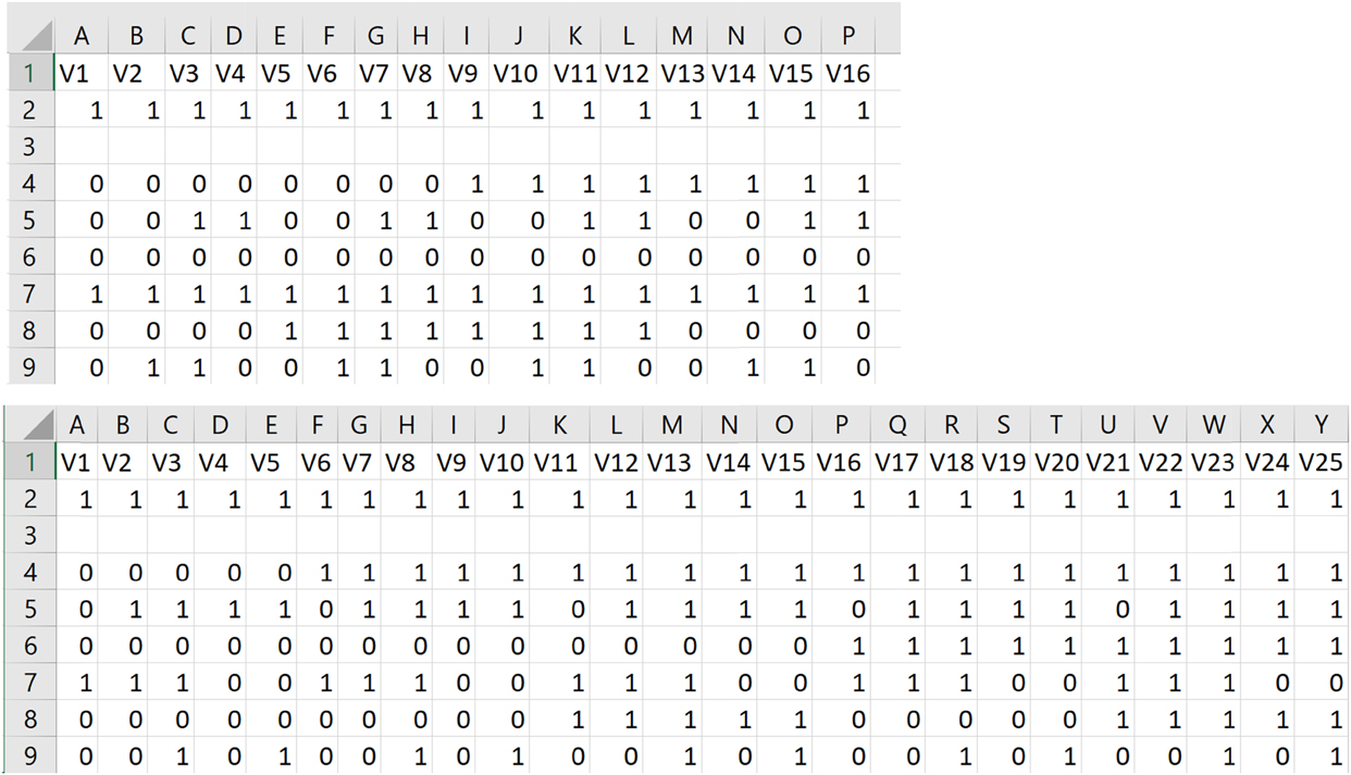
Input files for QTest giving the 16 preference patterns for CPT with overweighting and the 25 preference patterns for CPT with underweighting (see also Figure 2).

Appendix C
Proof
CPT with underweighting of small probabilities implies preference for Gamble R over Gamble S in Barron and Ursino’s Experiment 2 (see Table C1). More precisely, we prove that, according to CPT with 1 < δ ≤ 2 and 0 ≤ β ≤ 1
 $${w^ - }\left( {.15} \right) \times v\left( { - 20} \right) + \left( {1 - {w^ - }\left( {.15} \right)} \right) \times v\left( 0 \right) &gt; {w^ - }\left( 1 \right) \times v\left( { - 3} \right) + \left( {1 - {w^ - }\left( 1 \right)} \right) \times v\left( 0 \right).$$
Stimuli from Experiment 2 in Barron and Ursino (Reference Barron and Ursino2013)

Because w −(1) = 1 for all values of δ, since v(x) = −λ(−x)β, hence v(0) = 0 for all values of β, and, since, as we assumed, λ = 1 without loss in generality, we can rewrite Inequality 11 as
 $$\underbrace {{w^ - }\left( {.15} \right) \times \left( { - \left( {{{20}^{\rm{\beta }}}} \right)} \right)}_{{\rm{Left}} - {\rm{hand}}\,{\rm{side}}\,{\rm{of}}\,{\rm{Inequality}}\,12\,({\rm{LH}}{{\rm{S}}_{12}})} &gt; \underbrace { - \left( {{3^{\rm{\beta }}}} \right)}_{{\rm{Right}} - {\rm{hand}}\,{\rm{side}}\,{\rm{of}}\,{\rm{Inequality}}\,12\,({\rm{RH}}{{\rm{S}}_{12}})}.$$
From now on, we treat both LHS 12 and RHS 12 as functions of β on the range [0, 1] and we consider these for every fixed value of δ on the range (1, 2], and hence also for each resulting (fixed) value of w −(.15).
We begin by noting that w − (p) > 0 for any p > 0, which means that both LHS 12 and RHS 12 are power functions with a negative coefficient and an exponent β that varies on the range [0, 1]. It is known that power functions of this type are strictly decreasing and continuous, which makes both LHS 12 and RHS 12 strictly decreasing and continuous on 0 ≤ β ≤ 1 for any fixed value of δ. Given these properties of the LHS 12 and RHS 12, in order to prove Inequality 11, it is sufficient to prove the following two lemmas.
Lemma 1. The maximum value of LHS 12, for 0 ≤ β ≤ 1 and 1 < δ ≤ 2, is strictly greater than the maximum value of RHS 12, for 0 ≤ β ≤ 1 and 1 < δ ≤ 2.
Lemma 2. No matter what the values of 0 ≤ β ≤ 1 and 1 < δ ≤ 2 are, LHS 12 cannot equal RHS 12.
Proof of Lemma 1:
Since −(20β) and −(3β) are both strictly decreasing functions of β, for 0 ≤ β ≤ 1, they both attain their maximum values when β = 0, namely −(200) = −(30) = −1. Thus, Lemma 1 follows if we can show that w − (.15) × (−1) > −1. In other words, we need to show that w − (.15) < 1, regardless of 1 < δ ≤ 2. Instead, we even prove that w − (.15) < 0.15 for 1 < δ ≤ 2, and later use that result to prove Lemma 2.
First, we write out the inequality w − (.15) < 0.15 using the formula for the weighting function with δ, namely
 $${{{{\left( {{{15} \over {100}}} \right)}^{\rm{\delta }}}} \over {{{\left( {{{\left( {{{15} \over {100}}} \right)}^{\rm{\delta }}} + {{\left( {{{85} \over {100}}} \right)}^{\rm{\delta }}}} \right)}^{\left( {1/{\rm{\delta }}} \right)}}}} &lt; {{15} \over {100}}.$$
Reducing all component ratios in Inequality 13 gives
 $${{{{\left( {{3 \over {20}}} \right)}^{\rm{\delta }}}} \over {{{\left( {{{\left( {{3 \over {20}}} \right)}^{\rm{\delta }}} + {{\left( {{{17} \over {20}}} \right)}^{\rm{\delta }}}} \right)}^{\left( {1/{\rm{\delta }}} \right)}}}} &lt; {3 \over {20}}.$$
Factoring out 20 on the left turns Inequality 14 into
 $${1 \over {{{20}^{{\rm{\delta }} - 1}}}}{\rm{*}}{{{3^{\rm{\delta }}}} \over {{{\left( {{3^\delta } + {{17}^\delta }} \right)}^{\left( {{1 / {\rm{\delta }}}} \right)}}}} &lt; {3 \over {20}}.$$
Factoring out 3 on the left of Inequality 15 yields
 $${{{3^{{\rm{\delta }} - 1}}} \over {{{20}^{{\rm{\delta }} - 1}}}} \times {3 \over {{{\left( {{3^\delta } + {{17}^{\rm{\delta }}}} \right)}^{\left( {{1 / {\rm{\delta }}}} \right)}}}} &lt; {3 \over {20}}.$$
Multiplying both sides of Inequality 16 by  ${\left( {{3 \over {20}}} \right)^{1 - {\rm{\delta }}}}$ produces
 $${3 \over {{{\left( {{3^{\rm{\delta }}} + {{17}^{\rm{\delta }}}} \right)}^{\left( {{1 / {\rm{\delta }}}} \right)}}}} &lt; {3 \over {20}} \times {\left( {{3 \over {20}}} \right)^{1 - {\rm{\delta }}}}.$$
Exponentiating both sides of Inequality 17 by δ gives
 $$\underbrace {{{{3^{\rm{\delta }}}} \over {{3^\delta } + {{17}^{\rm{\delta }}}}}}_{LH{S_{18}}} &lt; \underbrace {{{\left( {{3 \over {20}}} \right)}^{\left( {2 - {\rm{\delta }}} \right){\rm{*\delta }}}}}_{RH{S_{18}}}.$$
Note that LHS 18 is strictly decreasing as a function of 1 < δ ≤ 2, whereas the RHS 18 is strictly increasing as a function of 1 < δ ≤ 2. Generally, LHS 18 = RHS 18 would imply that δ = 1. Since CPT with underweighting requires 1 < δ, therefore, LHS 18 < RHS 18 and, hence, w − (.15) < 0.15 for 1 < δ ≤ 2, which completes the proof of Lemma 1.
Proof of Lemma 2:
We use a proof by contradiction. Suppose that
 $${w^ - }\left( {.15} \right) \times - \left( {{{20}^{\rm{\beta }}}} \right) = - \left( {{3^{\rm{\beta }}}} \right).$$
Rearranging and simplifying terms gives
 $${w^ - }\left( {.15} \right) = {{{3^{\rm{\beta }}}} \over {{{20}^{\rm{\beta }}}}} = {0.15^{\rm{\beta }}}$$
We have already established that w − (.15) < 0.15 for 1 < δ ≤ 2. Since 0.15 ≤ 0.15β for 0 ≤ β ≤ 1 (by a line of argument similar to those earlier), it follows that Equation 20 cannot hold. This completes the proof of Lemma 2.
Appendix D
Proof
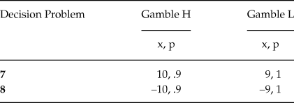
CPT with overweighting of small probabilities implies preference for Gamble L over H in Decision Problem 7 and Gamble H over L in Decision Problem 8 (see Table 6). More precisely, we prove that, for Decision Problem 7 according to CPT with 0 < γ < 1 and 0 ≤ β ≤ 1
 $${w^ + }\left( {.9} \right) \times v\left( {10} \right) + \left( {1 - {w^ + }(.9)} \right) \times v\left( 0 \right) &lt; {w^ + }\left( 1 \right) \times v\left( 9 \right) + \left( {1 - {w^ + }\left( 1 \right)} \right) \times v\left( 0 \right).$$
Our rationale for Decision Problem 8 is the same because the losses case is a mirror image of the gains case.
Decision Problems 7 and 8 from Barron and Erev (Reference Barron and Erev2003)

Because w + (1) = 1 for all values of γ, and since v(x) = (x)β hence v(0) = 0 for all values of β, we can rewrite Inequality 21 as
 $$\underbrace {{w^ + }\left( {.9} \right) \times \left( {{{10}^{\rm{\beta }}}} \right)}_{{\rm{Left}} - {\rm{hand}}\,{\rm{side}}\,{\rm{of}}\,{\rm{Inequality}}\,22\left( {{\rm{LH}}{{\rm{S}}_{22}}} \right)} &lt; \underbrace {{9^{\rm{\beta }}}}_{{\rm{Right}} - {\rm{hand}}\,{\rm{side}}\,{\rm{of}}\,{\rm{nequality}}\,22\left( {{\rm{RH}}{{\rm{S}}_{22}}} \right)}.$$
From now on, we treat both LHS 22 and RHS 22 as functions of β on the range [0, 1] and we consider these for every fixed value of γ on the range (0, 1), and hence also for each resulting (fixed) value of w + (.9).
We begin by noting that w + (p) > 0 for any p > 0, which means that both LHS 22 and RHS 22 are power functions with a positive coefficient and an exponent β that varies on the range [0, 1]. It is known that power functions of this type are strictly increasing and continuous, which makes both LHS 22 and RHS 22 strictly increasing and continuous on 0 ≤ β ≤ 1 for any fixed value of γ. Given these properties of the LHS 22 and RHS 22, in order to prove Inequality 21, it is sufficient to prove the following two lemmas.
Lemma 3. The maximum value of LHS 22, for 0 ≤ β ≤ 1 and 0 < γ < 1, is strictly smaller than the maximum value of RHS 22, for 0 ≤ β ≤ 1 and 0 < γ < 1.
Lemma 4. No matter what the values of 0 ≤ β ≤ 1 and 0 < γ < 1 are, LHS 22 cannot equal RHS 22.
Proof of Lemma 3:
Since 10β and 9β are both strictly increasing functions of β, for 0 ≤ β ≤ 1, they both attain their maximum values when β = 1, namely 10β = 10 and 9β = 9. Thus, Lemma 3 follows if we can show that w + (.9) × 10 < 9. In other words, we need to show that w + (.9) < .9, regardless of 0 < γ < 1.
First, we write out the inequality w + (.9) < 0.9 using the formula for the weighting function with γ, namely
 $${{{{\left( {{{90} \over {100}}} \right)}^{\rm{\gamma }}}} \over {{{\left( {{{\left( {{{90} \over {100}}} \right)}^{\rm{\gamma }}} + {{\left( {{{10} \over {100}}} \right)}^{\rm{\gamma }}}} \right)}^{\left( {{1 / {\rm{\gamma }}}} \right)}}}} &lt; {{90} \over {100}}.$$
Reducing all component ratios in Inequality 23 gives
 $${{{{\left( {{9 \over {10}}} \right)}^{\rm{\gamma }}}} \over {{{\left( {{{\left( {{9 \over {10}}} \right)}^{\rm{\gamma }}} + {{\left( {{1 \over {10}}} \right)}^{\rm{\gamma }}}} \right)}^{\left( {{1 / {\rm{\gamma }}}} \right)}}}} &lt; {9 \over {10}}.$$
Factoring out 10 on the left turns Inequality 24 into
 $${1 \over {{{10}^{{\rm{\gamma }} - 1}}}}{\rm{*}}{{{9^\gamma }} \over {{{\left( {{9^{\rm{\gamma }}} + {1^{\rm{\gamma }}}} \right)}^{\left( {{1 / {\rm{\gamma }}}} \right)}}}} &lt; {9 \over {10}}.$$
Factoring out 9 on the left of Inequality 25 yields
 $${{{9^{{\rm{\gamma }} - 1}}} \over {{{10}^{{\rm{\gamma }} - 1}}}} \times {9 \over {{{\left( {{9^{\rm{\gamma }}} + {1^{\rm{\gamma }}}} \right)}^{\left( {{1 / {\rm{\gamma }}}} \right)}}}} &lt; {9 \over {10}}.$$
Multiplying both sides of Inequality 26 by  ${\left( {{9 \over {10}}} \right)^{1 - {\rm{\gamma }}}}$ produces
 $${9 \over {{{({9^{\rm{\gamma }}} + {1^{\rm{\gamma }}})}^{\left( {{1 / {\rm{\gamma }}}} \right)}}}} &lt; {9 \over {10}} \times {\left( {{9 \over {10}}} \right)^{1 - {\rm{\gamma }}}}.$$
Exponentiating both sides of Inequality 27 by γ gives
 $$\underbrace {{{{9^{\rm{\gamma }}}} \over {{9^{\rm{\gamma }}} + {1^{\rm{\gamma }}}}}}_{LH{S_{28}}} &lt; \underbrace {{{\left( {{9 \over {10}}} \right)}^{\left( {2 - {\rm{\gamma }}} \right){\rm{*\gamma }}}}}_{RH{S_{28}}}.$$
Note that LHS 28 is strictly increasing as a function of 0 < γ < 1, whereas the RHS 28 is strictly decreasing as a function of 0 < γ < 1. Generally, max γ (LHS 28) = min γ (RHS 28) = 0.9 would imply that γ = 1. Since CPT with overweighting requires γ < 1, therefore, LHS 28 < RHS 28 and, hence, w + (.9) < 0.9 for 0 < γ < 1, which completes the proof for Lemma 3.
Proof of Lemma 4:
We use a proof by contradiction. Suppose that
 $${w^ + }\left( {.9} \right) \times \left( {{{10}^{\rm{\beta }}}} \right) = {9^{\rm{\beta }}}.$$
Rearranging and simplifying terms gives
 $${w^ + }\left( {.9} \right) = {{{9^{\rm{\beta }}}} \over {{{10}^{\rm{\beta }}}}} = {0.9^{\rm{\beta }}}$$
We have already established that w + (.9) < 0.9 for 0 < γ < 1. Since 0.9 ≤ 0.9β for 0 ≤ β ≤ 1 (by a line of argument similar to those earlier), it follows that Equation 30 cannot hold. This completes the proof of Lemma 4.