2.1. Formulations

The flow is governed by the momentum equation (Aleksandrova & Molokov Reference Aleksandrova and Molokov2004)

(2.1) \begin{equation} \frac {\partial \boldsymbol{u}}{\partial t}+(\boldsymbol{u} \boldsymbol{\cdot }\boldsymbol{\nabla }) \boldsymbol{u}=- \frac {1}{\rho } \boldsymbol{\nabla }{p}+ \nu {\nabla}^2 \boldsymbol{u}+\frac {1 }{\rho } \boldsymbol{j} \times \boldsymbol{B} - \boldsymbol{g}\beta (T-T_0), \end{equation}

and the mass conservation equation

(2.2) \begin{equation} \boldsymbol{\nabla }\boldsymbol{\cdot }\boldsymbol{u}=0. \end{equation}

Here, $\boldsymbol{u} =(u,v,w)$ , $\boldsymbol{j} = (j_x,j_y,j_z)$ are the velocity and electric current density of the fluid, $T$ is the temperature field, $\boldsymbol{B}=\boldsymbol{B}_0 + \boldsymbol{B}_i$ represents the magnetic induction (here we define $\boldsymbol{B_0}=(0,B_0,0)$ , $\boldsymbol{B_i}=(0,0,B_z^i)$ ), while $\boldsymbol{H} = (H_x,H_y,H_z)$ denotes the magnetic field which may also be considered as a current stream function. Also, $\rho$ represents the reference density of the fluid, $\nu$ is the kinematic viscosity, $\beta$ is the thermal expansion coefficient according to the Boussinesq approximation (Crapper & Baines Reference Crapper and Baines1977; De Les Valls et al. Reference De Les Valls, Sedano, Batet, Ricapito, Aiello, Gastaldi and Gabriel2008), $\sigma _{f}$ denotes the electric conductivity of the fluid and ${{\mu}} _f$ is permeability of the LM.

The current density is obtained by solving Ohm’s law

(2.3) \begin{equation} \boldsymbol{j}=\sigma _{f}(-\boldsymbol{\nabla }\phi +\boldsymbol{u} \times \boldsymbol{B}) , \end{equation}

Here $\phi$ denotes the electric potential, in conjunction with the charge conservation equation

(2.4) \begin{equation} \boldsymbol{\nabla }\boldsymbol{\cdot }\boldsymbol{j}=0 , \end{equation}

where

(2.5) \begin{equation} \boldsymbol{\nabla }\times \boldsymbol{H}= \boldsymbol{j} , \end{equation}

and

(2.6) \begin{equation} \boldsymbol{B}={\mu} _{\!f} \boldsymbol{H} . \end{equation}

The inductionless approximation is applied by assuming the magnetic Reynolds number ${\mathop {\textit{Re}}\nolimits }_m = \rho \sigma _{f} \nu l w_0$ is small enough, so that the induced field is negligible compared with the applied field when considering the magnetic field strength in the Lorentz force ( $\boldsymbol{B}_0 + \boldsymbol{B}_i \approx \boldsymbol{B}_0$ ). The momentum equation of fully established MHD mixed convection flow in a vertical duct driven by a pressure gradient $\partial p / \partial z$ combined with the buoyancy effect can then be expressed as

(2.7) \begin{equation} \nu \left ( \frac {\partial ^2 w}{\partial x^2} + \frac {\partial ^2 w}{\partial y^2} \right ) - \frac {1 }{\rho } \frac {\partial p}{\partial z} + \frac {1 }{\rho {\mu} _{\!f}} \frac {\partial B_z^i}{\partial y} B_0 + g\beta (T-T_0) = 0 , \end{equation}

and the governing equation of the induced magnetic field $\boldsymbol{B_i}$ satisfies the following form:

(2.8) \begin{equation} \frac {1}{{\mu} _{\!f} \sigma _f} \left( \frac {\partial ^2 B_z^i}{\partial x^2} + \frac {\partial ^2 B_z^i}{\partial y^2}\right) + B_0\frac {\partial w}{\partial y} = 0 . \end{equation}

The dimensionless, inductionless equations governing the problem can be expressed by means of the substitutions

(2.9) \begin{equation} \begin{aligned} x = l \bar {x}, \quad y = l \bar {y}, \quad &z = l \bar {z}, \quad w = w_0 \bar {w}, \quad \\[10pt] B_z^i = {\mu} _{\!f} \left (\partial p/\partial z\right ) l^2 \sqrt {\frac {\sigma _f}{\rho \nu }} \bar {b}, \quad &\bar {T} = \frac { T - \dfrac {1}{2}(T_h + T_c)}{ T_h - T_c } ,\end{aligned} \end{equation}

where the reference velocity is defined as (Prasad, Vaidya & Vajravelu Reference Prasad, Vaidya and Vajravelu2015)

(2.10) \begin{equation} w_0 = \frac {(\partial p/\partial z) l^2}{{\mu} _0}, \end{equation}

since the inertialess assumption is applied, the purely conductive temperature distribution in dimensionless notation is assumed to be linear. As shown in figure 1, $T_h$ and $T_c$ denote the constant temperature of the heating walls and the cooling walls, so that the temperature distribution can be expressed as $ \bar {T}= 1/2 - \bar {x}$ , with $\overline {\phantom {x}}$ distinguishing the dimensional quantity from the dimensionless counterpart. Equations (2.7) and (2.8) can be expressed non-dimensionally by means of these substitutions

(2.11) \begin{align} \frac {\partial ^2 \bar {w}}{ \partial \bar {x}^2} + \frac {\partial ^2 \bar {w}}{ \partial \bar {y}^2} + {\mathop {\textit{Ha}}\nolimits } \frac {\partial \bar {b}}{\partial \bar {y}} &= 1 - \frac {{\mathop {\textit{Gr}}\nolimits }}{{\mathop {\textit{Re}}\nolimits }} \bar {T}, \end{align}

(2.12) \begin{align} \frac {\partial ^2 \bar {b}}{ \partial \bar {x}^2} + \frac {\partial ^2 \bar {b}}{ \partial \bar {y}^2} + {\mathop {\textit{Ha}}\nolimits }\frac {\partial \bar {w}}{\partial \bar {y}} &= 0 . \end{align}

The non-dimensional parameters that characterise the flow are

(2.13) \begin{equation} {\mathop {\textit{Ha}}\nolimits } = Bl \sqrt {\frac {\sigma _f}{\rho \nu }} ,\quad {\mathop {\textit{Re}}\nolimits }= \frac {w_0l}{\nu },\quad {\mathop {\textit{Gr}}\nolimits } = \frac {g\beta \Delta T l^3}{\nu ^2}, \end{equation}

and ${{\mathop {\textit{Gr}}\nolimits }}/{{\mathop {\textit{Re}}\nolimits }}$ is defined as the mixed convection parameter here (Prasad et al. Reference Prasad, Vaidya and Vajravelu2015).

For a further analysis, all variables are composed of insulating solutions as in § 3, along with additional corrections that represent the influence of electrically conducting walls of arbitrary thickness and electrical conductivity

(2.14) \begin{equation} \left [\begin{array}{c} \boldsymbol{W} \\ \boldsymbol{b} \end{array}\right ] \rightarrow \left [\begin{array}{c} \boldsymbol{W_{\textit{ins}}} \\ \boldsymbol{b_{\textit{ins}}} \end{array}\right ]+\left [\begin{array}{c} \boldsymbol{W}_{\textit{hc}} \\ \boldsymbol{b}_{\textit{hc}} \end{array}\right ]+\left [\begin{array}{c} \boldsymbol{W}_{\textit{sc}} \\ \boldsymbol{b}_{\textit{sc}} \end{array}\right ]\!. \end{equation}

Here, the subscripts ( $_{\textit{ins}}$ ) denote the insulating solutions, ( $_{\textit{hc}}$ ) and ( $_{\textit{sc}}$ ) denote the electrical corrections to the insulated solutions for the finite conducting Hartmann walls and sidewalls. For all of the results considered below, ${\mu} _{\!f} /{\mu} _w = 1$ , $\sigma _f /\sigma _w = 1$ , where the subscript ( $_w$ ) denotes the parameters of the surrounding walls. Here, $\delta$ is used to represent the dimensionless thickness, as shown in figure 2, which is non-dimensionalised by the characteristic length $l$ . This includes both the Hartmann wall thickness and the sidewall thickness, with specific distinctions made using subscripts ( $_{hw}$ ) and ( $_{\textit{s}w}$ ). In this work, the channel is assumed to have a dimensionless constant flow rate of magnitude 1, the value of $\mathop {\textit{Re}}\nolimits$ was kept constant at 200 since we assumed the flow is laminar and the laminar solutions do not depend on $\mathop {\textit{Re}}\nolimits$ (Krasnov et al. Reference Krasnov, Boeck, Braiden, Molokov and Bühler2016).

3.1. Homogenisation of equations

To homogenise equation (2.11), the variables are decomposed into two parts by an auxiliary function $\boldsymbol{W_0}$ (velocity field) and $\boldsymbol{b_0}$ (magnetic field)

(3.1) \begin{equation} \left [\begin{array}{c} \boldsymbol{W_{\textit{ins}}} \\ \boldsymbol{b_{\textit{ins}}} \end{array}\right ] \rightarrow \left [\begin{array}{c} \boldsymbol{W_0} \\ \boldsymbol{b_0} \end{array}\right ]+\left [\begin{array}{c} \boldsymbol{W_i} \\ \boldsymbol{b_i} \end{array}\right ]\!, \end{equation}

here, $\boldsymbol{W_i} = (0,0,\bar {w_i})$ and $\boldsymbol{b_i} = (0,0,\bar {b_i} )$ represent the solutions of the homogenised equations.

Figure 2.

Schematic of case I (a), case II (b) and case III (c) in the $\bar {x}\bar {y}$ -plane. The parameters $\delta _{hw}^T$ and $\delta _{hw}^B$ represent the dimensionless thickness of the top and bottom Hartmann walls, while $\delta _{\textit{s}w}^R$ and $\delta _{\textit{s}w}^L$ represent the dimensionless thickness of the right and left sidewalls.

Firstly, for case I the fully established MHD flow in a rectangular duct with insulating walls is considered, as shown in figure 1. The wall at $\bar {x}=0$ is maintained at a constant temperature of $T_h = T_0/2$ , and the wall at $\bar {x}=1$ is maintained at a constant temperature of $T_c = -T_0/2$ , while the Hartmann walls are assumed adiabatic. The solutions satisfy no-slip conditions at the wall

(3.2) \begin{equation} \bar {w} =0 \quad \text{at} \quad \bar {x}=0, \ \bar {x}=1, \ \bar {y}=0, \ \bar {y}=1, \end{equation}

where the solid walls ( $\bar {x}=0, \ \bar {x}=1, \ \bar {y}=0, \ \bar {y}=1$ ) are assumed insulated, and the current boundary conditions satisfy

(3.3) \begin{equation} \begin{aligned} &J_x = \frac {1}{{\mu} _{\!f}} \frac {\partial\! B_z^i}{\partial y} \quad \text{at} \quad \bar {x}=0, \ \bar {x}=1,\\ &J_y = - \frac {1}{{\mu} _{\!f}} \frac {\partial\! B_z^i}{\partial x} \quad \text{at} \quad \bar {y}=0, \ \bar {y}=1, \end{aligned} \end{equation}

so the dimensionless induction $\bar {b}$ can be considered constant along the boundaries, and we set it to zero for simplicity, which can be written as

(3.4) \begin{equation} \bar {b}=0 \quad \text{at} \quad \bar {x}=0,\ \bar {x}=1,\ \bar {y}=0,\ \bar {y}=1. \end{equation}

As a consequence, the analytical solutions for MHD flows in a rectangular duct are derived by expressing the velocity $\bar {w}$ and the induced field $\bar {b}$ into Fourier series as (Shercliff Reference Shercliff1953)

(3.5) \begin{equation} \bar {w} = \sum _{n=1}^{\infty } W_n(\bar {y})\sin \left (\frac {n\pi }{l} \bar {x}\right )\!, \quad \bar {b} = \sum _{n=1}^{\infty } b_n(\bar {y})\sin \left (\frac {n\pi }{l} \bar {x}\right )\!, \end{equation}

where $W_n(\bar {y})$ and $b_n(\bar {y})$ are functions of $n$ and $\bar {y}$ , given that $\boldsymbol{b_0} = 0$ and $\boldsymbol{W_{\textit{ins}}} = \boldsymbol{W_0} + \boldsymbol{W_i}$ , and $\boldsymbol{W_0}$ satisfies the following governing equation:

(3.6) \begin{equation} \frac {\partial ^2 \bar {w}_0}{ \partial \bar {x}^2} = 1 - \frac {{\mathop {\textit{Gr}}\nolimits }}{{\mathop {\textit{Re}}\nolimits }} \bar {T}, \end{equation}

which satisfies the boundary conditions

(3.7) \begin{equation} \bar {w}_0=0 \quad {\textrm{at}} \quad \bar {x}=0, \ \bar {x}=1, \ \bar {y}=0, \ \bar {y}=1. \end{equation}

Here, the right-hand term in (3.6) can be expressed as a Fourier series over the range $\bar {x} \in [0, 1]$ (where $\bar {T} = 1/2 -\bar {x}$ )

(3.8) \begin{equation} 1 - \frac {{\mathop {\textit{Gr}}\nolimits }}{{\mathop {\textit{Re}}\nolimits }} \bar {T} = \sum _{n=1}^{\infty } \left[ \left(- \frac {{\mathop {\textit{Gr}}\nolimits }}{{\mathop {\textit{Re}}\nolimits }} + 2 \right) \left( -\frac {\cos (n\pi )}{n\pi } + \frac {1}{n \pi } \right) + 2\frac {{\mathop {\textit{Gr}}\nolimits }}{{\mathop {\textit{Re}}\nolimits }} \left(-\frac {\cos (n\pi )}{n\pi }\right) \right] \sin (n \pi \bar {x}), \end{equation}

and consequently, the auxiliary function $\bar {w}_0$ can be expressed as

(3.9) \begin{equation} \begin{aligned} \bar {w}_0= \sum _{n=1}^{\infty } W_0(n) \sin (n \pi \bar {x}) & = \sum _{n=1}^{\infty } \frac {-1}{n^2 \pi ^2} \left[ \left(- \frac {{\mathop {\textit{Gr}}\nolimits }}{{\mathop {\textit{Re}}\nolimits }} + 2 \right) \left( -\frac {\cos (n\pi )}{n\pi } + \frac {1}{n \pi } \right) \right.\\[6pt] &\quad \left. +\, \left(2\frac {{\mathop {\textit{Gr}}\nolimits }}{{\mathop {\textit{Re}}\nolimits }}\right) \left(-\frac {\cos (n\pi )}{n\pi }\right) \right] \sin (n \pi \bar {x}), \end{aligned} \end{equation}

where $W_0(n)$ is a coefficient dependent on n.

3.2. The analytical solution for case I

Then the governing equation of $w_i$ can be expressed as

(3.10) \begin{align} \frac {\partial ^2 \bar {w}_i}{ \partial \bar {x}^2} + \frac {\partial ^2 \bar {w}_i}{ \partial \bar {y}^2} + {\mathop {\textit{Ha}}\nolimits }\frac {\partial \bar {b}_i}{\partial \bar {y}} &= 0, \end{align}

(3.11) \begin{align} \frac {\partial ^2 \bar {b}_i}{ \partial \bar {x}^2} + \frac {\partial ^2 \bar {b}_i}{ \partial \bar {y}^2} + {\mathop {\textit{Ha}}\nolimits } \frac {\partial \bar {w}_i}{\partial \bar {y}} &= 0. \end{align}

Combining equation (2.12), it is convenient to introduce the Elsasser variables to express the velocity and fluid magnetic fields to decouple the governing equations

(3.12) \begin{equation} \Phi = \bar {w}_i + \bar {b}_i,\quad \Psi = \bar {w}_i - \bar {b}_i . \end{equation}

By applying the Elsasser’s variables that listed in (3.12), equations (3.11) and (2.12) can be rewritten as

(3.13) \begin{align} \frac {\partial ^2 \Phi }{ \partial \bar {x}^2} + \frac {\partial ^2 \Phi }{ \partial \bar {y}^2} + {\mathop {\textit{Ha}}\nolimits }\frac {\partial \Phi }{\partial \bar {y}} &= 0 , \end{align}

(3.14) \begin{align} \frac {\partial ^2 \Psi }{ \partial \bar {x}^2} + \frac {\partial ^2 \Psi }{ \partial \bar {y}^2} - {\mathop {\textit{Ha}}\nolimits }\frac {\partial \Psi }{\partial \bar {y}} &= 0. \end{align}

The boundary conditions corresponding to no-slip and insulated walls for case I on $\Phi$ and $\Psi$ satisfy

(3.15) \begin{align} \Phi +\Psi =-2 \bar {w}_0, \ {\textrm{at}} \ \bar {y}=0, \ \bar {y}=1, &\ \quad \Phi +\Psi =-2 \bar {w}_0, \ {\textrm{at}} \ \bar {x}=0, \ \bar {x}=1 , \end{align}

(3.16) \begin{align} \Phi -\Psi =0, \ {\textrm{at}}\ \bar {y}=0, \ \bar {y}=1 , &\ \quad \Phi -\Psi =0, \ {\textrm{at}}\ \bar {x}=0, \ \bar {x}=1. \end{align}

The general solutions which satisfy the Dirichlet boundary conditions on all walls can be expressed as

(3.17) \begin{equation} \Phi = \sum _{n=1}^\infty \! \big(A_{1}(n) e^{r_1 \bar {y}}+B_{1}(n) e^{r_2 \bar {y}}\big) \!\sin (n\pi \bar {x}), \quad \! \Psi = \sum _{n=1}^\infty \! \big(A_{2}(n) e^{r_3 \bar {y}}+B_{2}(n) e^{r_4 \bar {y}}\big) \! \sin (n\pi \bar {x}), \end{equation}

where

(3.18) \begin{equation} r_{1,2}=\frac {-H a \pm \sqrt {H a^2+4 n^2 \pi ^2}}{2} , \quad r_{3,4}=\frac {H a \pm \sqrt {H a^2+4 n^2 \pi ^2}}{2} , \end{equation}

and the coefficients by applying $u_n^0 = - W_0(n)$ satisfy the following forms:

(3.19) \begin{equation} \begin{aligned} &A_{1}(n)=\frac {u_n^0 e^{r_2}-u_n^0}{e^{r_2}-e^{r_1}}, \quad B_{1}(n)=\frac {u_n^0 e^{r_1}-u_n^0}{e^{r_1}-e^{r_2}},\\[8pt] &A_{2}(n)=\frac {u_n^0 e^{r_4}-u_n^0}{e^{r_4}-e^{r_3}}, \quad B_{2}(n)=\frac {u_n^0 e^{r_3}-u_n^0}{e^{r_3}-e^{r_4}}. \end{aligned} \end{equation}

Subsequently, the solutions of the Fourier modes of the velocity and induced magnetic field solutions for the fluid (see (3.11)) can be easily written as follows:

(3.20) \begin{align} \bar {w}_i &= \sum _{n=1}^\infty F_i(n,\bar {y}) \sin (n \pi \bar {x}) \nonumber\\ &= \frac {1}{2} \sum _{n=1}^\infty \big( A_{1}(n) e^{r_1 \bar {y}}+B_{1}(n) e^{r_2 \bar {y}} + A_{2}(n) e^{r_3 \bar {y}} +B_{2}(n) e^{r_4 \bar {y}}\big) \sin (n \pi \bar {x}), \end{align}

(3.21) \begin{align} \bar {b}_i &= \sum _{n=1}^\infty P_i(n,\bar {y}) \sin (n \pi \bar {x}) \nonumber\\ &= \frac {1}{2} \sum _{n=1}^\infty \big( A_{1}(n) e^{r_1 \bar {y}}+B_{1}(n) e^{r_2 \bar {y}} - A_{2}(n) e^{r_3 \bar {y}} -B_{2}(n) e^{r_4 \bar {y}}\big) \sin (n \pi \bar {x}) , \end{align}

where $F_i(n,\bar {y})$ and $P_i(n,\bar {y})$ are functions of $n$ and $\bar {y}$ .

3.3. Result and discussion

An accurate analytical solution for calculating mixed convection flow in an insulated duct is derived in $\S$ 3.2. This vertical insulated duct is influenced by an additional horizontal magnetic field and a horizontal temperature difference. It reveals fluid flow behaviour under varying ${{\mathop {\textit{Gr}}\nolimits }}/{{\mathop {\textit{Re}}\nolimits }}$ , delineating three convection states – forced convection at very low $ {{\mathop {\textit{Gr}}\nolimits }}/{{\mathop {\textit{Re}}\nolimits }}$ values ( $ ({{\mathop {\textit{Gr}}\nolimits }}/{{\mathop {\textit{Re}}\nolimits }}) \ll 1$ ), buoyancy-dominated convection at very high $ {{\mathop {\textit{Gr}}\nolimits }}/{{\mathop {\textit{Re}}\nolimits }}$ values ( $ ( {{\mathop {\textit{Gr}}\nolimits }}/{{\mathop {\textit{Re}}\nolimits }}) \gg 1$ ) and mixed convection phenomena when $ {{\mathop {\textit{Gr}}\nolimits }}/{{\mathop {\textit{Re}}\nolimits }}$ 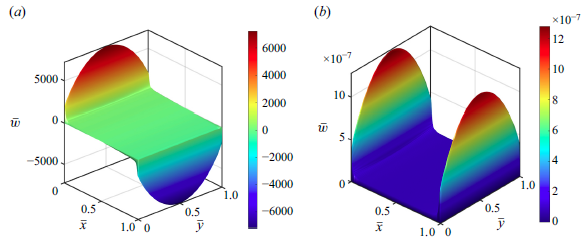is at an intermediate level. The accuracy of this analytical solution is validated by comparison with classical cases proposed by Shercliff (Reference Shercliff1953) and Tagawa et al. (Reference Tagawa, Authié and Moreau2002). Results shown in figure 3 indicate the high accuracy of the analytical solution for both MHD forced convection (left part of figure 3) and MHD buoyancy-dominated convection (right part of figure 3).

Figure 3.

Comparison of analytical with results proposed by Shercliff (Reference Shercliff1953) (a) and Tagawa et al. (Reference Tagawa, Authié and Moreau2002) (b) of velocity profile for ${\mathop {\textit{Ha}}\nolimits } = 100$ along $\bar {x}=0.5$ and $\bar {y} = 0.5$ .

Reverse flow is a critical phenomenon in mixed convection, especially in breeding blankets, where inflection point instability can trigger magnetoconvective fluctuations (Zikanov et al. Reference Zikanov, Belyaev, Listratov, Frick, Razuvanov and Sviridov2021). The occurrence of reverse flow is closely linked to the mixed convection number ( $ {{\mathop {\textit{Gr}}\nolimits }}/{{\mathop {\textit{Re}}\nolimits }}$ ), with results shown in figure 4. These results indicate that, as $ {{\mathop {\textit{Gr}}\nolimits }}/{{\mathop {\textit{Re}}\nolimits }}$ increases, buoyancy effects become more pronounced, leading to an increasing velocity gradient aligned with the temperature gradient. As demonstrated in figure 5, a critical threshold is identified under the inertialess assumption at $( {{\mathop {\textit{Gr}}\nolimits }}/{{\mathop {\textit{Re}}\nolimits }})_{c} = 2$ . Reverse flow emerges when $ {{\mathop {\textit{Gr}}\nolimits }}/{{\mathop {\textit{Re}}\nolimits }}$ exceeds this critical value ( $ ({{\mathop {\textit{Gr}}\nolimits }}/{{\mathop {\textit{Re}}\nolimits }}) \gt ( {{\mathop {\textit{Gr}}\nolimits }}/{{\mathop {\textit{Re}}\nolimits }})_{c}$ ), and the formation of an inflection point at this transition may induce instability and a shift to turbulence even at lower $\mathop {\textit{Re}}\nolimits$ (Zikanov et al. Reference Zikanov, Belyaev, Listratov, Frick, Razuvanov and Sviridov2021). It should be noted that, in order to ensure that the dimensionless flow rate is fixed at 1, the dimensionless temperature has been converted to $\bar {T} = 1/Q(1/2 - \bar {x})$ here.

Figure 4.

Comparison of velocity contours (a,b,c) and current streamlines (d,e,f) at different $ {{\mathop {\textit{Gr}}\nolimits }}/{{\mathop {\textit{Re}}\nolimits }}$ : (a,d) ( $ ({{\mathop {\textit{Gr}}\nolimits }}/{{\mathop {\textit{Re}}\nolimits }}) \ll 1$ ), (b,e) ( $ ({{\mathop {\textit{Gr}}\nolimits }}/{{\mathop {\textit{Re}}\nolimits }}) \sim 1$ ) and (c,f) ( $ ({{\mathop {\textit{Gr}}\nolimits }}/{{\mathop {\textit{Re}}\nolimits }}) \gg 1$ ) for ${\mathop {\textit{Ha}}\nolimits }=100$ .

The detailed flow characteristics at various $ {{\mathop {\textit{Gr}}\nolimits }}/{{\mathop {\textit{Re}}\nolimits }}$ values are depicted in figures 4 and 5. As illustrated in figure 4, when $ ({{\mathop {\textit{Gr}}\nolimits }}/{{\mathop {\textit{Re}}\nolimits }}) \ll 1$ the velocity profile exhibits typical Shercliff flow characteristics, with the maximum velocity occurring in the central region of the duct and decreasing near the surrounding wall, resulting in a symmetric distribution. This occurs because $\mathop {\textit{Gr}}\nolimits$ is relatively low, allowing MHD forced convection to exert a dominant influence. In this regime, the current lines roll into two counter-rotating loops that symmetric about the $\bar {y} = 0.5$ line. When $ {{\mathop {\textit{Gr}}\nolimits }}/{{\mathop {\textit{Re}}\nolimits }}$ is at a moderate value, mixed convection mechanism dominates, and the velocity gradient in the core region satisfies the results provided by Tagawa et al. (Reference Tagawa, Authié and Moreau2002). In this work, it can be rewritten as

(3.22) \begin{equation} \frac {\partial {\bar {w}} }{\partial {\bar {x}}}\sim \frac {{\mathop {\textit{Gr}}\nolimits }}{2{\mathop {\textit{Re}}\nolimits }{\mathop {\textit{Ha}}\nolimits }}. \end{equation}

This is because the velocity gradient in mixed convection is still decided by the combining the effect of the buoyancy and Lorentz forces. A similar scaling also exists in the case of conductive walls (as shown on the right side of figure 5), with the detailed derivation provided in § 5. As $ {{\mathop {\textit{Gr}}\nolimits }}/{{\mathop {\textit{Re}}\nolimits }}$ increases further to $ ({{\mathop {\textit{Gr}}\nolimits }}/{{\mathop {\textit{Re}}\nolimits }}) \gg 1$ , buoyancy-dominated convection gradually becomes the dominant mechanism and the horizontal temperature gradient generates an upward forced flow around the heating wall and a reversed flow near the cooling wall, providing a stable stratification. Under these conditions, the current lines evolve into four loops corresponding to this downstream and upstream subsequently.

Figure 5.

Velocity profile for case I along $\bar {y}=0.5$ at ${\mathop {\textit{Ha}}\nolimits }=100$ , for various $ {{\mathop {\textit{Gr}}\nolimits }}/{{\mathop {\textit{Re}}\nolimits }}$ for case I (a) and the velocity profile for case III, with all the walls possessing uniform thickness and the walls’ thickness equal to 0.1 ( $ \delta _{hw} =\delta _{\textit{s}w} =0.1$ ) along $\bar {y}=0.5$ (b).

Additionally, $\mathop {\textit{Ha}}\nolimits$ serves as a crucial governing parameter that determines the flow pattern, particularly for the distribution of the boundary layer. Results for both forced convection and buoyancy-dominated convection are presented in figure 6. When $ ({{\mathop {\textit{Gr}}\nolimits }}/{{\mathop {\textit{Re}}\nolimits }}) \ll 1$ , the flow is predominantly driven by the pressure gradient, with the forced convection mechanism taking precedence. As depicted in the left part of figure 6, an increase in $\mathop {\textit{Ha}}\nolimits$ intensifies the magnetic damping effects, which suppresses the core flow region and leads to a thinning of the side boundary layer, with thickness scaling as $\sim\!{\mathop{\textit{Ha}}\nolimits }^{-({1}/{2})}$ . In the case of buoyancy-dominated convection, as $\mathop {\textit{Ha}}\nolimits$ increases, the current lines become more concentrated in the boundary layer region, resulting in an increase in the peak velocity of the boundary layer and a reduction in its thickness, as similarly observed by (Müller et al. Reference Müller and Bühler2001).

Figure 6.

Velocity profiles along $\bar {y}=0.5$ for various $\mathop {\textit{Ha}}\nolimits$ : forced convection at $ ({{\mathop {\textit{Gr}}\nolimits }}/{{\mathop {\textit{Re}}\nolimits }}) \ll 1$ (a), buoyancy-dominated convection at $ ({{\mathop {\textit{Gr}}\nolimits }}/{{\mathop {\textit{Re}}\nolimits }}) \gg 1$ (b).

4.1. Governing equations and boundary conditions

The influence of electrically conducting Hartmann wall with arbitrary thickness and electrical conductivity is considered in this case (case II) and the detailed geometric configuration is shown in figure 2. For further analysis, the velocity field $\boldsymbol{W}$ and magnetic field $\boldsymbol{b}$ are further decomposed as

(4.1) \begin{equation} \left [\begin{array}{c} \boldsymbol{W} \\ \boldsymbol{b} \end{array}\right ] \rightarrow \left [\begin{array}{c} \boldsymbol{W_{\textit{ins}}} \\ \boldsymbol{b_{\textit{ins}}} \end{array}\right ]+\left [\begin{array}{c} \boldsymbol{W}_{\textit{hc}} \\ \boldsymbol{b}_{\textit{hc}} \end{array}\right ]\!. \end{equation}

Hence, the governing equations of $\boldsymbol{W}_{\textit{hc}} = (0,0,\bar {w}_{\textit{hc}})$ and $\boldsymbol{b}_{\textit{hc}} = (0,0,\bar {b}_{\textit{hc}})$ can be subsequently decoupled and rewritten as

(4.2) \begin{align} \frac {\partial ^2 \Phi _{\textit{hc}}}{ \partial \bar {x}^2} + \frac {\partial ^2 \Phi _{\textit{hc}} }{ \partial \bar {y}^2} + {\mathop {\textit{Ha}}\nolimits }\frac {\partial \Phi _{\textit{hc}}}{\partial \bar {y}} &= 0 , \end{align}

(4.3) \begin{align} \frac{\partial^2 \Psi_{hc}}{ \partial \bar{x}^2} + \frac{\partial^2 \Psi_{hc} }{ \partial \bar{y}^2} - Ha \frac{\partial \Psi_{hc}}{\partial \bar{y}} = 0, \end{align}

where

(4.4) \begin{equation} \Phi _{\textit{hc}} = \bar {w}_{\textit{hc}} + \bar {b}_{\textit{hc}},\quad \Psi _{\textit{hc}} = \bar {w}_{\textit{hc}} -\bar {b}_{\textit{hc}} . \end{equation}

To solve the region of walls that possess arbitrary thickness and electrical conductivity, the governing equation for the induced magnetic field is considered, which can be written as follows (Tao & Ni Reference Tao and Ni2015) (Bluck & Wolfendale Reference Bluck and Wolfendale2015):

(4.5) \begin{equation} {\nabla}^2 \bar {b}_{hw}^T = 0,\quad {\nabla}^2 \bar {b}_{hw}^B = 0 , \end{equation}

where the superscripts ( $^B$ ) and ( $^T$ ) denote the values that induced by the bottom Hartmann wall and top Hartmann wall, the subscript ( $_{hw}$ ) denotes the values of the solid region at the Hartmann wall. For the boundary conditions, the induced magnetic field is assumed to be continuous at the interface of the fluid flow and the conducting walls (Tao & Ni Reference Tao and Ni2015)

(4.6) \begin{equation} \bar {b}= \bar {b}_{\textit{hc}}+\bar {b}_0+\bar {b}_i = \frac {{\mu} _{\!f}}{{\mu} _{hw}} \bar {b}_{hw} \quad {\textrm{at}} \quad \bar {y}=0,\ \bar {y}=1 , \end{equation}

while the electrical current has continuous tangential components at the fluid–wall interface (Tao & Ni Reference Tao and Ni2015)

(4.7) \begin{equation} \frac {\partial \bar {b}}{\partial \bar {y}}=\frac {\partial \left (\bar {b}_{\textit{hc}}+\bar {b}_0+\bar {b}_i\right ) }{\partial \bar {y}} =\frac {{\mu} _{\!f} \sigma _{f}}{{\mu} _{hw} \sigma _{hw}} \frac {\partial \bar {b}_{hw}}{\partial \bar {y}} \quad {\textrm{at}} \quad \bar {y}=0,\ \bar {y}=1 . \end{equation}

Sidewalls are considered to be insulated and Robin boundary conditions are applied to the induced magnetic field at Hartmann walls. For velocity field, no-slip boundary conditions are applied at all surrounding walls, so for $\Phi _{\textit{hc}}$ and $\Psi _{\textit{hc}}$ the boundary conditions satisfy

(4.8) \begin{equation} \begin{aligned} & \Phi _{\textit{hc}}-\Psi _{\textit{hc}}=2 \bar {b}_{\textit{hc}}, \quad \frac {\partial (\Phi _{\textit{hc}}-\Psi _{\textit{hc}})}{ \partial \bar {y} } = 2\frac {\partial \bar {b}_{\textit{hc}}}{ \partial \bar {y}} , \quad \textrm{at}\ \bar {y}=0, \\[4pt] & \Phi _{\textit{hc}}-\Psi _{\textit{hc}}=2 \bar {b}_{\textit{hc}}, \quad \frac {\partial (\Phi _{\textit{hc}}-\Psi _{\textit{hc}})}{ \partial \bar {y} } = 2\frac {\partial \bar {b}_{\textit{hc}}}{ \partial \bar {y}},\quad \textrm{at}\ \bar {y}=1, \\ & \Phi _{\textit{hc}}-\Psi _{\textit{hc}}=0, \quad \textrm{at}\ \bar {x}=0, \ \bar {x}=1, \\ & \Phi _{\textit{hc}}+\Psi _{\textit{hc}}=0, \quad \textrm{at}\ \bar {y}=0, \ \bar {y}=1,\\ & \Phi _{\textit{hc}}+\Psi _{\textit{hc}}=0, \quad \textrm{at}\ \bar {x}=0, \ \bar {x}=1. \end{aligned} \end{equation}

4.2. The analytical solution for case II

The general solutions of magnetic field in the solid region for the conducting Hartmann wall that satisfy the interface conditions (see (4.6), (5.7)), as well as the insulated wall boundary conditions of the outer surfaces, can be written as

(4.9) \begin{equation} \begin{aligned} \bar {b}_{hw}^B &=\sum _{n=1}^{\infty } b_{n}^B(n) \sinh \big(n \pi \big(\bar {y} + \delta _{hw}^B\big)\big)\sin (n \pi \bar {x}) \quad {\textrm{at}} \quad \bar {y} \in \big[{-}\delta _{hw}^B,0\big],\\ \bar {b}_{hw}^T &=\sum _{n=1}^{\infty } b_{n}^T(n) \sinh \big(n \pi \big(\bar {y} - 1 - \delta _{hw}^T\big)\big)\sin (n \pi \bar {x}) \quad {\textrm{at}} \quad \bar {y} \in \big[1, 1 + \delta _{hw}^T \big], \end{aligned} \end{equation}

where $b_{n}^B(n)$ and $b_{n}^T(n)$ are coefficients dependent on $n$ .

The general solutions for the influence of finite conducting Hartmann walls in MHD pressure-driven flow is detailed discussed in Tao & Ni (Reference Tao and Ni2015) and Bluck & Wolfendale (Reference Bluck and Wolfendale2015). In this case, the analytical solutions for the conducting effect’s part of MHD mixed convection is expressed as follows:

(4.10) \begin{equation} \begin{aligned} \Phi _{\textit{hc}} & =\sum _{n=1}^{\infty } \big[ T_1(n) e^{-\frac {{\mathop {\textit{Ha}}\nolimits }}{2} \bar {y}} \sinh (\eta \bar {y}) - T_2(n) e^{-\frac {{\mathop {\textit{Ha}}\nolimits }}{2} \bar {y}} \sinh (\eta (\bar {y}-1))\big]\sin (n \pi \bar {x}) ,\\ \Psi _{\textit{hc}} & =\sum _{n=1}^{\infty } \big[T_3(n) e^{\frac {{\mathop {\textit{Ha}}\nolimits }}{2} \bar {y}} \sinh (\eta \bar {y}) -T_4(n) e^{\frac {{\mathop {\textit{Ha}}\nolimits }}{2} \bar {y}} \sinh (\eta (\bar {y}-1))\big] \sin (n \pi \bar {x}) ,\\ \end{aligned} \end{equation}

where $\eta = \sqrt {{\mathop {\textit{Ha}}\nolimits }^2/4 + n^2 \pi ^2}$ , combined with the no-slip conditions in all walls ( $\bar {w}_{\textit{hc}} = 0$ at $\bar {y}=0,\ \bar {y}=1$ ), and it is convenient to write

(4.11) \begin{align} \bar {b}_{\textit{hc}} &= \sum _{n=1}^{\infty } \left[T_2(n) \cosh \left(\frac {{\mathop {\textit{Ha}}\nolimits }}{2} \bar {y}\right) \sinh (\eta (1-\bar {y})) \right. \nonumber\\ &\quad \left. +\, T_1(n) e^{-\frac {{\mathop {\textit{Ha}}\nolimits }}{2}} \cosh \left(\frac {{\mathop {\textit{Ha}}\nolimits }}{2}(1-\bar {y})\right) \sinh (\eta \bar {y})\right]\sin (n \pi \bar {x}), \end{align}

(4.12) \begin{align} \bar {w}_{\textit{hc}} &= \sum _{n=1}^{\infty } \left[T_2(n) \sinh \left(\frac {{\mathop {\textit{Ha}}\nolimits }}{2} \bar {y}\right) \sinh (\eta (1-\bar {y})) \right. \nonumber\\ &\quad \left. +\, T_1(n) e^{-\frac {{\mathop {\textit{Ha}}\nolimits }}{2}} \sinh \left(\frac {{\mathop {\textit{Ha}}\nolimits }}{2}(1-\bar {y})\right) \sinh (\eta \bar {y})\right]\sin (n \pi \bar {x}) . \\[8pt] \nonumber \end{align}

The solutions for the Fourier modes of velocity and the induced magnetic field within the fluid can then be readily derived as follows:

(4.13) \begin{align} T_1(n) &= e^{\frac {{\mathop {\textit{Ha}}\nolimits }}{2}} \frac {\left[N_1^B(n) N_2^B(n)+N_4(n)\right] \frac {\partial P_i}{\partial \bar{y}}(n,1)-N_3(n) \frac {\partial P_i}{\partial \bar{y}}(n,0)}{N_3(n)^2- \left[N_4(n)+N_1^T(n) N_2^T(n)\right]\left[N_4(n)+N_1^B(n) N_2^B(n)\right]},\\[-12pt]\nonumber\end{align}

(4.14) \begin{align} T_2(n) &= \frac {\left[N_1^T(n) N_2^T(n)+N_4(n)\right] \frac {\partial P_i}{\partial \bar{y}}(n,0)-N_3(n) \frac {\partial P_i}{\partial \bar{y}}(n,1)}{\left[N_4(n)+N_1^T(n) N_2^T(n)\right]\left[N_4(n)+N_1^B(n) N_2^B(n)\right]-N_3(n)^2} , \end{align}

where $P_i$ is an abbreviation for the coefficient $P_i(n, \bar {y})$ defined in (3.21), and

(4.15) \begin{equation} \begin{aligned} & N_1^B(n)= \frac {{\mu} _{hw}^B}{{\mu} _{\!f}} \frac {\sinh (\eta )}{\sinh \left (n \pi \delta _{hw}^B\right )}, \qquad\qquad\,\, N_1^T(n)= \frac {{\mu} _{hw}^T}{{\mu} _{\!f}} \frac {\sinh (\eta )}{\sinh \left (n \pi \delta _{hw}^T\right )}, \\[6pt] & N_2^B(n)=\frac {{\mu} _{\!f} \sigma _{f}}{{\mu} _{hw}^B \sigma _{hw}^B} n \pi \cosh \big(n \pi \delta _{hw}^B\big), \quad N_2^T(n)=\frac {{\mu} _{\!f} \sigma _{f}}{{\mu} _{hw}^T \sigma _{hw}^T} n \pi \cosh \big(n \pi \delta _{hw}^T\big), \\[6pt] & N_3(n)= \eta \cosh \left(\frac {{\mathop {\textit{Ha}}\nolimits }}{2}\right)\!, \quad N_4(n)= \eta \cosh (\eta ). \end{aligned} \end{equation}

4.3. Result and discussion

Building on the findings from case I, we examine a scenario where Robin boundary conditions (i.e. finite conductivity) are applied at the Hartmann walls, while Dirichlet boundary conditions (insulating walls) are imposed at the sidewalls. The solution of this part is based on the work of Tao & Ni (Reference Tao and Ni2015) and Bluck & Wolfendale (Reference Bluck and Wolfendale2015); when the Grashof number ( $\mathop {\textit{Gr}}\nolimits$ ) approaches zero, the analytical result (see figure 7) shows excellent agreement with solution proposed by Bluck & Wolfendale (Reference Bluck and Wolfendale2015), as anticipated. The introduction of electrically conductive Hartmann walls draws the current lines closer to the sidewalls, allowing some of the current to close through these walls due to the induced potential gradient. Consequently, this adjustment raises the current density in the core region, significantly intensifying the electric potential gradient. This alteration further suppresses the core flow velocity under the Lorentz force, while the side-layer region remains comparatively unaffected, resulting in the emergence of characteristic jet structures.

Figure 7.

Comparison of analytical solution from this work with results by Bluck & Wolfendale (Reference Bluck and Wolfendale2015) for velocity distribution along $\bar {x} = 0.5$ and $\bar {y} = 0.5$ for ${\mathop {\textit{Ha}}\nolimits } = 100$ and $\delta _{hw} = 0.05$ .

Figure 8.

Asymmetric distribution of velocity (a) and current streamlines on induced magnetic field distribution contour (b) with $ \delta _{hw}^T = 0.5$ and $ \delta _{hw}^B = 0.01$ .

Additionally, since both upper and lower Hartmann walls are solved, the analytical solution is extended to account for an asymmetric wall conductivity case. As illustrated in figure 8, a particular case is considered in which the top Hartmann wall is markedly thicker compared with the bottom wall, with $\delta _{hw}^T = 0.5$ and $\delta _{hw}^B = 0.01$ . As anticipated, the majority of the electric current lines tend to be drawn to close through the top wall because of the high wall conductance ratio (where $c_{hw} = ({\sigma _{hw} \delta _{hw}})/{\sigma _f l}$ ), leaving only a minor portion passing through the relatively less conductive bottom wall. This results in an asymmetric velocity profile along $\bar {y}$ -direction and its variation with $\delta _{hw}^T$ is thoroughly illustrated in figure 9. By varying the thickness of the top wall while keeping the bottom wall fixed, the velocity distribution along the line $\bar {x} = 0.5$ is extracted to evaluate the influence of wall thickness on the flow characteristics. As the wall conductance ratio ( $c_{hw} = ({\sigma _{hw} \delta _{hw}})/{\sigma _f l}$ ) increases, the current lines density around the bulk region becomes larger because of the lower resistance, and the magnitude of the velocity presents to be reduced around the highly conducting wall, thus causing an unsymmetrical distribution.

Figure 9.

Velocity profile at $\bar {x} = 0.5$ for ${\mathop {\textit{Ha}}\nolimits } = 100$ and $ ({{\mathop {\textit{Gr}}\nolimits }}/{{\mathop {\textit{Re}}\nolimits }}) \sim 1$ , with varying $\delta _{hw}^T$ values.

Figure 10.

Variation of pressure drop with $\mathop {\textit{Ha}}\nolimits$ and $c_{hw}$ (a), pressure drop as a function of $\mathop {\textit{Ha}}\nolimits$ with varying $c_{hw}$ (b) for $ ({{\mathop {\textit{Gr}}\nolimits }}/{{\mathop {\textit{Re}}\nolimits }}) \sim 1$ .

To properly design the LM loop and optimise the flow path within the blanket, it is crucial to accurately estimate the MHD pressure drop (Tassone et al. Reference Tassone, Siriano, Caruso, Utili and Del Nevo2020). Since the dimensionless volumetric flow rate Q can be obtained by an integration of the velocity field, and the pressure drop can be given by $ ({\partial \bar {p}}/{\partial \bar {z}}) = 1/Q$ , to evaluate the pressure drop under fusion reactor conditions at high Hartmann numbers, the solutions of this part can be reformulated using the method proposed by Ni et al. (Reference Ni, Munipalli, Morley, Huang and Abdou2007b ). The combined influence of wall thickness (conductivity ratio) and $\mathop {\textit{Ha}}\nolimits$ on the pressure gradient under symmetric Hartmann walls is illustrated in figure 10, where it is demonstrated that the increase of both wall thickness and $\mathop {\textit{Ha}}\nolimits$ can result in a further increase in the pressure gradient, and these factors interact with each other. Power laws of

(4.16) \begin{equation} \frac {\partial \bar {p}}{\partial \bar {z}} \sim {\mathop {\textit{Ha}}\nolimits }^{q}, \end{equation}

can be applied for this case and can be seen in the right part of figure 10. Here, $q$ is a coefficient that characterises the scaling of the pressure gradient with respect to $\mathop {\textit{Ha}}\nolimits$ . Due to interaction between the fluid and conducting walls, $q$ is highly related to $c_{hw}$ and it increases with the thickening of the Hartmann walls. We consider an extreme case by an asymptotic expansion for $Q$ when $c_{hw} \to \infty$ as ${\mathop {\textit{Ha}}\nolimits } \to \infty$ in terms of $1/{\mathop {\textit{Ha}}\nolimits }$

(4.17) \begin{equation} Q = \int _{0}^{1} \int _{0}^{1} (\bar {w}_0 + \bar {w}_i + \bar {w}_{\textit{hc}}) \, {\textrm{d}}\bar {x} {\textrm{d}}\bar {y}, \end{equation}

neglecting smaller terms, $Q$ can then be written as

(4.18) \begin{align} Q & = \int _{0}^{1} \sum _{n = 0}^{\infty } u_n^0 \left( 1 - \frac {2\eta }{M^2 - \eta ^2} \frac {e^{M -\eta } - 1}{1 - e^{-2\eta }} - \frac {2}{\eta ^2 - M^2} \frac {\left (1 - e^{M - \eta } \right )\left(M - \eta e^{M - \eta }\right)}{e^{M - \eta } + 1}\right) \nonumber\\& \quad\times\, \sin (n \pi \bar {x})\, {\textrm{d}}\bar {x}, \end{align}

where $M = {\mathop {\textit{Ha}}\nolimits }/2$ . By employing the Williams (Reference Williams1963) method, and directly expanding of the equation in conjunction with the Taylor remainder theorem and the Poisson summation formula, it can be deduced that the leading term is $O({\mathop {\textit{Ha}}\nolimits }^{-({3}/{2})})$ as ${\mathop {\textit{Ha}}\nolimits } \to \infty$ and $c_{hw} \to \infty$ . While, for the scenarios where the Hartmann walls exhibit arbitrary thickness and electrical conductivity, the dependence of $q$ on the $\mathop {\textit{Ha}}\nolimits$ demonstrates a distinct behaviour that is shown on the right bottom of figure 10: as the conductivity ratio of the Hartmann walls $c_{hw}$ transitions from 0 to infinity, the value of $q$ follows a non-monotonic trend where it initially increases from $1$ to reach a peak value of nearly $1.9$ and then subsequently decreases to $1.5$ . This can also be explained by directly expansions. If the wall thickness is thin enough with $\delta _{hw} \ll 1$ , the items of solutions can the be written as

(4.19) \begin{equation} N_1^B(n)N_2^B(n) = N_1^T(n)N_2^T(n)= \frac {\sigma _f \boldsymbol{\cdot }1}{\sigma _{hw} \delta _{hw}} = \frac {1}{c_{hw}} , \end{equation}

where $c_{hw}$ is defined as the Hartmann walls’ conductance ratio. So for finite conducting Hartmann walls, the dimensionless volumetric flow rate satisfies the following form:

(4.20) \begin{equation} Q = f_1\frac {1}{1 + c_{hw} {\mathop {\textit{Ha}}\nolimits }} \frac {1}{{\mathop {\textit{Ha}}\nolimits }} +f_2 \frac {1}{1 + c_{hw} {\mathop {\textit{Ha}}\nolimits }} \frac {1}{{\mathop {\textit{Ha}}\nolimits }^{3/2}} +f_3 \frac {c_{hw}{\mathop {\textit{Ha}}\nolimits }}{1 + c_{hw} {\mathop {\textit{Ha}}\nolimits }} \frac {1}{{\mathop {\textit{Ha}}\nolimits }^{3/2}} + O\left(\frac {1}{{\mathop {\textit{Ha}}\nolimits }^2}\right)\!, \end{equation}

where $f_1,\ f_2,\ f_3$ are constant terms and can be easily obtained by the method proposed by Williams (Reference Williams1963).

5.1. Governing equations and boundary conditions

For the further analysis, additional corrections that represent the influence of electrically conducting sidewalls with arbitrary thickness and electrical conductivity are introduced

(5.1) \begin{equation} \left [\begin{array}{c} \boldsymbol{W} \\ \boldsymbol{b} \end{array}\right ] \rightarrow \left [\begin{array}{c} \boldsymbol{W_{\textit{ins}}} \\ \boldsymbol{b_{\textit{ins}}} \end{array}\right ]+\left [\begin{array}{c} \boldsymbol{W}_{\textit{hc}} \\ \boldsymbol{b}_{\textit{hc}} \end{array}\right ]+\left [\begin{array}{c} \boldsymbol{W}_{\textit{sc}} \\ \boldsymbol{b}_{\textit{sc}} \end{array}\right ]\!, \end{equation}

and the decomposed velocity $\boldsymbol{W}_{\textit{hc}} = (0,0,\bar {w}_{\textit{sc}})$ and magnetic field $\boldsymbol{b}_{\textit{hc}} = (0,0,\bar {b}_{\textit{sc}})$ are further analysed without applying the thin-wall approximation. Robin boundary conditions are imposed on the magnetic field at both the Hartmann and sidewalls, and the governing equations deduced by (2.11) and (2.12) can be expressed as follows:

(5.2) \begin{align} \frac {\partial ^2 \bar {w}_{\textit{sc}}}{ \partial \bar {x}^2} + \frac {\partial ^2 \bar {w}_{\textit{sc}}}{ \partial \bar {y}^2} + {\mathop {\textit{Ha}}\nolimits }\frac {\partial \bar {b}_{\textit{sc}}}{\partial \bar {y}} &= 0 , \end{align}

(5.3) \begin{align} \frac {\partial ^2 \bar {b}_{\textit{sc}}}{ \partial \bar {x}^2} + \frac {\partial ^2 \bar {b}_{\textit{sc}}}{ \partial \bar {y}^2} + {\mathop {\textit{Ha}}\nolimits }\frac {\partial \bar {w}_{\textit{sc}}}{\partial \bar {y}} &= 0 . \\[6pt] \nonumber \end{align}

The governing equation for the induced magnetic field of the sidewall region is considered, which can be written as follows:

(5.4) \begin{equation} {\nabla}^2 \bar {b}_{\textit{s}w}^T = 0,\quad {\nabla}^2 \bar {b}_{\textit{s}w}^B = 0 , \end{equation}

and Robin boundary conditions for the magnetic are applied to ensure the continuity of the electric current at the interface of the sidewalls; the induced magnetic field should also be kept smooth here. The corresponding boundary conditions are given as follows:

(5.5) \begin{align} \bar {b} &=\bar {b}_{\textit{sc}}+\bar {b}_{\textit{hc}}+\bar {b}_0+\bar {b}_i = \frac {{\mu} _{\!f}}{{\mu} _{\textit{s}w}} \bar {b}_{\textit{s}w} \quad {\textrm{at}} \quad \bar {x}=0,\ \bar {x}=1 , \end{align}

(5.6) \begin{align} \frac {\partial \bar {b}}{\partial \bar {x}} &=\frac {\partial \left (\bar {b}_{\textit{sc}}+\bar {b}_{\textit{hc}}+\bar {b}_0+\bar {b}_i\right ) }{\partial \bar {x}} =\frac {{\mu} _{\!f} \sigma _{f}}{{\mu} _{\textit{s}w} \sigma _{\textit{s}w}} \frac {\partial \bar {b}_{\textit{s}w}}{\partial \bar {x}} \quad {\textrm{at}} \quad \bar {x}=0,\ \bar {x}=1 . \end{align}

Considering the Hartmann walls are highly electrically conducting, the influence of $\bar {b}_{\textit{sc}}$ on (4.6) is assumed to be negligible, and will not impact that around Hartmann walls (Bühler Reference Bühler1998), so we assume

(5.7) \begin{equation} \frac {\partial \bar {b}_{\textit{sc}} }{\partial \bar {y}} = 0 \quad {\textrm{at}} \quad \bar {y}=0,\bar {y}=1 . \end{equation}

Combined with the no-slip conditions, the analytical solution for the MHD mixed convection component induced by the conducting sidewalls is derived by expressing the velocity $\bar {w}_{\textit{sc}}$ and the induced magnetic field $\bar {b}_{\textit{sc}}$ as Fourier series expansions, as follows:

(5.8) \begin{equation} \begin{aligned} &\bar {w}_{\textit{sc}}=\sum _{n=0}^{\infty } W_{\textit{scn}}(n,\bar {x}) \sin \left (n \pi \bar {y}\right )\!, \quad \bar {b}_{\textit{sc}}=\sum _{n=0}^{\infty } b_{\textit{scn}}(n,\bar {x}) \cos \left (n \pi \bar {y}\right )\!, \\ \end{aligned} \end{equation}

where $W_{\textit{scn}}$ and $b_{\textit{scn}}$ are functions of $n$ and $\bar {x}$ . For the magnetic field in the solid region

(5.9) \begin{equation} \begin{aligned} \bar {b}_{\textit{s}w}^L &=\sum _{n=1}^{\infty } b_{n}^L(n) \sinh \big(n \pi \big(\bar {x} + \delta _{\textit{s}w}^L\big)\big)\cos (n \pi \bar {y}) \quad {\textrm{at}} \quad \bar {x} \in \big[-\delta _{\textit{s}w}^L,0\big],\\ \bar {b}_{\textit{s}w}^R &=\sum _{n=1}^{\infty } b_{n}^R(n) \sinh \big(n \pi \big(\bar {y} - 1 - \delta _{\textit{s}w}^R\big)\big)\cos (n \pi \bar {y}) \quad {\textrm{at}} \quad \bar {x} \in \big[1, 1 + \delta _{\textit{s}w}^R\big], \end{aligned} \end{equation}

where $b_{n}^L(n)$ and $b_{n}^R(n)$ are coefficients dependent on $n$ . By substituting the Fourier modes of $\bar {w}_{\textit{sc}}$ and $\bar {b}_{\textit{sc}}$ into the momentum and charge conservation equations (5.2) and (5.3), the governing equations can then be rewritten as

(5.10) \begin{align} \frac {\partial ^2 \bar {w}_{\textit{sc}}}{\partial \bar {x}^2}-n^2 \pi ^2 \bar {w}_{\textit{sc}}-{\mathop {\textit{Ha}}\nolimits } n \pi \bar {b}_{\textit{sc}} &=0,\\[-6pt]\nonumber\end{align}

(5.11) \begin{align} \frac {\partial ^2 \bar {b}_{\textit{sc}}}{\partial \bar {x}^2}-n^2 \pi ^2 \bar {b}_{\textit{sc}}+{\mathop {\textit{Ha}}\nolimits } n \pi \bar {w}_{\textit{sc}} &=0. \end{align}

We decouple the velocity and magnetic fields through the Elsasser variables $\Phi _{\textit{sc}}$ and $\Psi _{\textit{sc}}$

(5.12) \begin{align} \Phi _{\textit{sc}}=\bar {w}_{\textit{sc}}+\bar {b}_{\textit{sc}} i ,\quad \Psi _{\textit{sc}}=\bar {w}_{\textit{sc}}-\bar {b}_{\textit{sc}} i , \end{align}

where $\lambda = n \pi$ , and $\Phi _{\textit{sc}}$ and $\Psi _{\textit{sc}}$ satisfy

(5.13) \begin{align} \frac{\partial^2 \Phi_{sc}}{\partial \bar{x}^2}-\left(\lambda^2- Ha \lambda i\right) \Phi_{sc}=0 ,\\[-6pt]\nonumber\end{align}

(5.14) \begin{align} \frac{\partial^2 \Psi_{sc}}{\partial \bar{x}^2}-\left(\lambda^2+Ha \lambda i\right) \Psi_{sc}=0 .\end{align}

Assuming that the Hartmann walls are highly conducting, the correct solution of conducting sidewalls will not affect the potential at the Hartmann walls (Bühler Reference Bühler1998). As for the induced magnetic field, it corresponds to $\partial \bar {b}_{\textit{sc}} /\partial \bar {y} = 0$ . The induced field and the tangential components of the electric field are continuous at the fluid–wall interface (see (5.5) and (5.6)), combined with the no-slip boundary condition at all surrounding walls, the boundary conditions for $\Phi _{\textit{sc}}$ and $\Psi _{\textit{sc}}$ can be written as

(5.15) \begin{eqnarray} &\phi _{\textit{sc}}+\psi _{\textit{sc}}=0,\quad \bar {y}=0, \ \bar {y}=1 ,\nonumber\\[3pt] &\phi _{\textit{sc}}+\psi _{\textit{sc}}=0,\quad \bar {x}=0, \ \bar {x}=1 ,\nonumber\\[3pt] &\phi _{\textit{sc}}-\psi _{\textit{sc}}=2 \bar {b}_{\textit{sc}}i,\quad \dfrac {\partial (\phi _{\textit{sc}}-\psi _{\textit{sc}})}{ \partial \bar {x} } = 2\dfrac {i\partial \bar {b}_{\textit{sc}}}{ \partial \bar {x}},\quad \bar {x}=0 ,\\[3pt] &\phi _{\textit{sc}}-\psi _{\textit{sc}}=2 \bar {b}_{\textit{sc}}i,\quad \dfrac {\partial (\phi _{\textit{sc}}-\psi _{\textit{sc}})}{ \partial \bar {x} } = 2\dfrac {i\partial \bar {b}_{\textit{sc}}}{ \partial \bar {x}},\quad \bar {x}=1 ,\nonumber\\[3pt] &\dfrac {\partial (\phi _{\textit{sc}}-\psi _{\textit{sc}})} { \partial \bar {y}}=0,\quad \bar {y}=0, \ \bar {y}=1 . \nonumber \end{eqnarray}

Due to the highly conducting assumption applied to Hartmann walls, the interface conditions along $\bar {y} = 0$ and $\bar {y} = 1$ (see (4.6)) are altered due to the introduction of $\bar {b}_{\textit{sc}}$ . As a consequence, a correction of induced magnetic field $\bar {b}_{cr}$ is adopted in the region of Hartmann walls, and the highly conducting assumption is also applied to the two sidewalls when solving these solid regions

(5.16) \begin{equation} \begin{aligned} &\bar {b}^B_{cr} = \sum _{n=1}^{n} \left ( \frac {b^B_\textit{crn}(n)}{\sinh \left(n\pi \delta _{hw}^B\right)} \boldsymbol{\cdot }\sinh \big(n\pi \big(\bar {y} + \delta _{hw}^B\big)\big) \boldsymbol{\cdot }\cos (n\pi \bar {x}) \right )\!,\\[4pt] &\bar {b}^T_{cr}= \sum _{n=1}^{n} \left ( \frac {-b^T_\textit{crn}(n)}{\sinh \left(n\pi \delta _{hw}^T\right)} \boldsymbol{\cdot }\sinh \big(n\pi \big(\bar {y} - \delta _{hw}^T - 1\big)\big) \boldsymbol{\cdot }\cos (n\pi \bar {x}) \right )\!, \end{aligned} \end{equation}

where the subscript ( $_{cr}$ ) represents the correction term, and $b^B_\textit{crn}(n)$ and $b^T_\textit{crn}(n)$ are coefficients dependent on $n$ .

5.2. The analytical solution for case III

It is straightforward to write the general solutions for $n \gt 1$ of MHD flows in a rectangular duct with sidewalls of arbitrary thickness and electrical conductivity as equation (5.8) and

(5.17) \begin{align} W_{\textit{scn}}(n,\bar {x}) &=\left (S_1(n) \sinh (\beta \bar {x})+S_2(n) \sinh (\beta (\bar {x}-1))\right ) \cos (r \bar {x}) \nonumber\\ &\quad +\left (S_3(n) \sinh (\beta \bar {x})+S_4(n) \sinh (\beta (\bar {x}-1))\right ) \sin (r \bar {x}),\\[-6pt]\nonumber\end{align}

(5.18) \begin{align} b_{\textit{scn}}(n,\bar {x}) &= [- \left ( S_1(n) \cosh (\beta \bar {x}) + S_2(n) \cosh (\beta (\bar {x}-1))\right ) \sin (r \bar {x}) \nonumber\\ &\quad + \left (S_3(n) \cosh (\beta \bar {x})+S_4(n) \cosh (\beta (\bar {x}-1))\right ) \cos (r \bar {x})] , \\[6pt] \nonumber \end{align}

where

(5.19) \begin{equation} \beta =\left (\frac {1}{2} \lambda \right )^{\frac {1}{2}}\Big (\sqrt {\lambda ^2+H a^2}+\lambda \Big )^{\frac {1}{2}} ,\quad r=\left (\frac {1}{2} \lambda \right )^{\frac {1}{2}}\Big (\sqrt {\lambda ^2+H a^2}-\lambda \Big )^{\frac {1}{2}}\! . \end{equation}

The coefficients in the equations can be written as

(5.20) \begin{eqnarray} && N_R(n)=\frac {\sigma _{f}^R}{\sigma _{\textit{s}w}^R} n \pi \frac {\cosh \left(n\pi \delta _{\textit{s}w}^R\right)}{\sinh \left(n \pi \delta _{\textit{s}w}^R\right)} ,\quad N_L(n)=\frac {\sigma _{f}^L}{\sigma _{\textit{s}w}^L} n \pi \frac {\cosh \left(n\pi \delta _{\textit{s}w}^L\right)}{\sinh \left(n \pi \delta _{\textit{s}w}^L\right)} ,\nonumber\\[5pt] && \,\, F_1(n)=\cosh \beta \sin r + \frac {\cosh \beta \cos r}{\tan r} ,\nonumber\\[5pt] && \, F_2(n)=\left(r\cos r - \frac {r}{\tan r}\sin r\right)\cosh \beta + \beta \sinh \beta \left(\sin r + \frac {\cos r}{\tan r}\right)\! ,\nonumber\\[5pt] && \, S_1(n) = \nonumber\\ && \frac {M_1(n)\left(N_L(n)\cosh \beta + \beta \sinh \beta \right) + M_0(n)(N_R(n)\cos r - r\sin r)}{(-N_R(n)F_1(n) - F_2(n))(-N_L(n)\cosh \beta \!-\! \beta \sinh \beta )\!-\!(N_R(n)\cos r \!-\! r\sin r) \!\left(\frac {N_L(n)}{\tan r}\!-\!r\! \right)},\nonumber\\ && S_2(n) = 0,\nonumber\\ && S_3(n) = -\frac {1}{\tan r} S_1(n),\nonumber\\ && S_4(n) = \nonumber\\ && \frac {- M_1(n)\left(\frac {N_L(n)}{\tan r}-r\right) + M_0(n)(-N_R(n)F_1(n) \!-\! F_2(n))}{(N_R(n)\cos r \!-\! r\sin r) \!\left(\frac {N_L(n)}{\tan r}\!-\!r\! \right) \!-\! (-N_R(n)F_1(n)-F_2(n))(-N_L(n)\cosh \beta \!-\! \beta \sinh \beta )}. \nonumber\\ \end{eqnarray}

The solutions for $n=0$ are

(5.21) \begin{equation} b_{\textit{sc}}(\bar {x}) = C_0 \bar {x} + D_0, \quad W_{\textit{sc}}(\bar {x}) = 0, \end{equation}

where

(5.22) \begin{equation} \begin{aligned} & C_0 = \frac {\displaystyle\frac {\sigma _{f} \delta _{\textit{s}w}^L}{\sigma _{\textit{s}w}^L} M_0(0) + \displaystyle\frac {\sigma _{f} \delta _{\textit{s}w}^R}{\sigma _{\textit{s}w}^R} M_1(0)}{-1 - \displaystyle\frac {\sigma _{f} \delta _{\textit{s}w}^L}{\sigma _{\textit{s}w}^L} - \displaystyle\frac {\sigma _{f} \delta _{\textit{s}w}^R}{\sigma _{\textit{s}w}^R}} ,\\ & D_0 = \displaystyle\frac {\sigma _{f} \delta _{\textit{s}w}^L}{\sigma _{\textit{s}w}^L} C_0 + \displaystyle\frac {\sigma _{f} \delta _{\textit{s}w}^R}{\sigma _{\textit{s}w}^R} M_0(0), \end{aligned} \end{equation}

where $M_1(n)$ and $M_0(n)$ represent the cosine expansion coefficients of $\partial \bar {b} / \partial \bar {x}$ obtained by the result of case II at $\bar {x}=1$ and $\bar {x}=0$ .

Figure 11.

Validation of analytical and numerical results for the velocity profile with all the walls possessing uniform thickness at $ \delta _{hw} =\delta _{\textit{s}w} =0.1$ : for buoyancy-dominated flow at various $\mathop {\textit{Ha}}\nolimits$ values $ ({{\mathop {\textit{Gr}}\nolimits }}/{{\mathop {\textit{Re}}\nolimits }}) \gg 1$ (a), for mixed convection at ${\mathop {\textit{Ha}}\nolimits } = 100$ and $ ({{\mathop {\textit{Gr}}\nolimits }}/{{\mathop {\textit{Re}}\nolimits }}) \sim 1$ (b).

5.3. Result and discussion

Our analytical solution demonstrates strong agreement with the recent numerical studies (Akhtari, Zikanov & Krasnov Reference Akhtari, Zikanov and Krasnov2024) for buoyancy-dominated flows (as shown in the left part of figure 11), across Hartmann numbers ranging from 325 to 796 with the four surrounding walls’ conductance ratio set to 0.1. And for mixed convection schemes where ${\mathop {\textit{Ha}}\nolimits }=100$ , $ ({{\mathop {\textit{Gr}}\nolimits }}/{{\mathop {\textit{Re}}\nolimits }}) \sim 1$ and $\delta = 0.1$ for all surrounding walls, the analytical solution also shows great agreement with the numerical results obtained by the MHD-UCAS platform in the right part of figure 11, particularly in predicting the velocity and current distribution within the system that includes electrically conducting walls. In the mixed convection schemes, the velocity field (see figure 12) retains the characteristic jet-like profile, with the core flow exhibiting a typical linear distribution induced by the temperature gradient in the $\bar {x}$ -direction, while the peak velocity of the side-layer jet is reduced and the velocity of the core flow becomes faster due to the introduction of the conducting sidewalls compared with case II. This is because, in this scenario, unlike case II, the electrically conducting sidewalls allow the current loops that are shown in figure 13 to close through the solid regions near the side boundary layers, thereby impacting the current density distribution, which results in a weaker suppression of the core flow by the Lorentz force and a decrease in the peak velocity of the jet in the side layers.

Figure 12.

Velocity contour (a) and the distribution of current streamlines with induced magnetic field (b) for ${\mathop {\textit{Ha}}\nolimits } = 100$ , $ ({{\mathop {\textit{Gr}}\nolimits }}/{{\mathop {\textit{Re}}\nolimits }}) \sim 1$ , and all the walls possessing uniform thickness at $ \delta _{hw} =\delta _{\textit{s}w} =0.1$ .

Figure 13.

Distribution of current streamlines including solid region with induced magnetic field for ${\mathop {\textit{Ha}}\nolimits } = 100$ , $ ({{\mathop {\textit{Gr}}\nolimits }}/{{\mathop {\textit{Re}}\nolimits }}) \sim 1$ and $\delta _{hw}=\delta _{\textit{s}w}=0.1$ .

The interaction between the magnetic field and the conducting Hartmann walls leads to the formation of high-velocity jets near the sidewalls, which are susceptible to flow instability (Kinet, Knaepen & Molokov Reference Kinet, Knaepen and Molokov2009; Krasnov et al. Reference Krasnov, Boeck, Braiden, Molokov and Bühler2016). Additionally, stable stratification caused by the buoyancy effect and the generation of the inflection points may lead to the instability at very low $\mathop {\textit{Re}}\nolimits$ (Zikanov et al. Reference Zikanov, Belyaev, Listratov, Frick, Razuvanov and Sviridov2021). The fully established laminar axial velocity profiles under different convection schemes is also important to understand the development trend as $\mathop {\textit{Re}}\nolimits$ increases. Three distinct flow regimes – forced convection ( $ ({{\mathop {\textit{Gr}}\nolimits }}/{{\mathop {\textit{Re}}\nolimits }}) \ll 1$ ), mixed convection ( $ ({{\mathop {\textit{Gr}}\nolimits }}/{{\mathop {\textit{Re}}\nolimits }}) \sim 1$ ) and buoyancy-dominated convection ( $ ({{\mathop {\textit{Gr}}\nolimits }}/{{\mathop {\textit{Re}}\nolimits }}) \gg 1$ ) are investigated for ${\mathop {\textit{Ha}}\nolimits } = 100$ and $ \delta _{hw} =\delta _{\textit{s}w} =0.1$ , and the results are presented in figure 14. In the forced convection regime with conducting Hartmann walls and sidewalls ( $\delta _{\textit{s}w} = 0.1$ ), a typical symmetric M-shaped velocity profile of MHD flow is observed, where the peak velocities near both sidewalls are almost identical, and the core flow exhibits a nearly uniform velocity distribution which is mainly driven by the pressure gradient. As the $ {{\mathop {\textit{Gr}}\nolimits }}/{{\mathop {\textit{Re}}\nolimits }}$ increases to moderate values, buoyancy effects become significant, inducing asymmetry in the velocity profile. This results in higher jet velocities near the heated wall compared with the cooler one. By extending results proposed by Tagawa et al. (Reference Tagawa, Authié and Moreau2002) for purely buoyancy-driven flow in insulated ducts to mixed convection within electrically conductive ducts, a constant velocity gradient which can be scaled as $ |{\partial \bar {w}}/{\partial \bar {x}}| \sim ({{\mathop {\textit{Gr}}\nolimits }})/({2{\mathop {\textit{Re}}\nolimits }{\mathop {\textit{Ha}}\nolimits }(1 + c{\mathop {\textit{Ha}}\nolimits })})$ is deduced. Here, the effect of the conducting sidewall on the velocity gradient in the core flow is negligible.

Figure 14.

Comparison of velocity contours and current streamlines with $ \delta _{hw} =\delta _{\textit{s}w} =0.1$ for different $ {{\mathop {\textit{Gr}}\nolimits }}/{{\mathop {\textit{Re}}\nolimits }}$ : (a,d) ( $ ({{\mathop {\textit{Gr}}\nolimits }}/{{\mathop {\textit{Re}}\nolimits }}) \ll 1$ ), (b,e) ( $ ({{\mathop {\textit{Gr}}\nolimits }}/{{\mathop {\textit{Re}}\nolimits }})\sim 1$ ) and (c,f) ( $ ({{\mathop {\textit{Gr}}\nolimits }}/{{\mathop {\textit{Re}}\nolimits }})\gg 1$ ) for ${\mathop {\textit{Ha}}\nolimits }=100$ .

The governing equation in Tagawa et al. (Reference Tagawa, Authié and Moreau2002) can be written as

(5.23) \begin{equation} \Delta \bar {w} + {\mathop {\textit{Ha}}\nolimits }\bar {J_x} + \frac {{\mathop {\textit{Gr}}\nolimits }}{{\mathop {\textit{Re}}\nolimits }}\bar {T} - 1 = 0, \end{equation}

where $\bar {J_x}$ represents the x-component of the dimensionless electric current. The solutions of the core flow satisfy

(5.24) \begin{equation} \begin{aligned} \bar {\phi }^0 &= -\frac {{\mathop {\textit{Gr}}\nolimits }}{{\mathop {\textit{Re}}\nolimits }{\mathop {\textit{Ha}}\nolimits }}\int _{0}^{y} \int _{0}^{y'} \frac {\partial \bar {T}}{\partial \bar {x}} {\textrm{d}}y {\textrm{d}}y' + Y \boldsymbol{\cdot }G(x) + H(x) ,\\ \bar {w}^0 &= \frac {1}{{\mathop {\textit{Ha}}\nolimits }}\left(\frac {{\mathop {\textit{Gr}}\nolimits }}{{\mathop {\textit{Re}}\nolimits }{\mathop {\textit{Ha}}\nolimits }}\bar {T} - \frac {1}{{\mathop {\textit{Ha}}\nolimits }} - yG'(x) - H'(x)\right)\! , \end{aligned} \end{equation}

where the superscript ( $^0$ ) denotes the quantities within the core and $\bar {\phi }^0$ denotes the dimensionless electric potential within the core flow. Together with the thin-wall assumption and current boundary condition, we get

(5.25) \begin{equation} G(X) = -\frac {{\mathop {\textit{Gr}}\nolimits }}{2{\mathop {\textit{Re}}\nolimits }{\mathop {\textit{Ha}}\nolimits }}, \quad H''(x) = \frac {1}{1+c{\mathop {\textit{Ha}}\nolimits }}\left(\frac {{\mathop {\textit{Gr}}\nolimits }}{2{\mathop {\textit{Re}}\nolimits }} - \frac {{\mathop {\textit{Gr}}\nolimits }}{{\mathop {\textit{Ha}}\nolimits } {\mathop {\textit{Re}}\nolimits }}\right)\!, \end{equation}

and then we assume the $\mathop {\textit{Ha}}\nolimits$ is high enough and the conducting wall is thin, so that the velocity gradient of the core flow can be deduced as

(5.26) \begin{equation} \frac {\partial \bar {w}^0}{ \partial \bar {x}} = - \frac {{\mathop {\textit{Gr}}\nolimits }}{2{\mathop {\textit{Re}}\nolimits }{\mathop {\textit{Ha}}\nolimits }(1+c{\mathop {\textit{Ha}}\nolimits })}. \end{equation}

When $ {{\mathop {\textit{Gr}}\nolimits }}/{{\mathop {\textit{Re}}\nolimits }}$ further increases, reverse jet formation is observed near the cooling wall due to the buoyancy effect, and the velocity here is significantly high due to the MHD effect and raises questions about potential instability for high $\mathop {\textit{Re}}\nolimits$ at critical points which can be seen in figure 5. For this specific case, $( {{\mathop {\textit{Gr}}\nolimits }}/{{\mathop {\textit{Re}}\nolimits }})_c = 2$ , as mentioned in § 3.3.

Figure 15.

Velocity profile variation for different $\mathop {\textit{Ha}}\nolimits$ values along $\bar {y}=0.5$ (a) and $\bar {x}=0.5$ (b) for $ ({{\mathop {\textit{Gr}}\nolimits }}/{{\mathop {\textit{Re}}\nolimits }}) \sim 1$ and $ \delta _{hw} =\delta _{\textit{s}w} =0.1$ .

The impact of increasing $\mathop {\textit{Ha}}\nolimits$ on the velocity profiles is investigated for MHD mixed convection with arbitrary electrically conducting walls ( $\delta _{hw} = \delta _{\textit{s}w} = 0.1$ ) at $ {{\mathop {\textit{Gr}}\nolimits }}/{{\mathop {\textit{Re}}\nolimits }} \sim 1$ . As shown in figure 15, an increase in $\mathop {\textit{Ha}}\nolimits$ leads to an enhanced magnetic confinement corresponding to a reduction in the core flow velocity and the thinning of the side-layer jets with rising peak values.

This analytical solution demonstrates great performance in cases of asymmetric electrically conducting walls for both the side and Hartmann walls, as shown in figure 16. In this case, the top Hartmann wall and the left sidewall possess higher conductivity with thick walls ( $\delta _{hw}^T=0.5,\ \delta _{\textit{s}w}^L=0.5$ ), while the remaining walls are maintained at thinner wall thickness ( $\delta _{hw}^ B=0.1,\ \delta _{\textit{s}w}^R=0.1$ ). Figure 16 reveals the detailed non-uniform flow distribution caused by the influence of this asymmetric configuration. As can be seen, the left sidewall with higher conductivity causes the current lines to travel through the left solid region more easily, as the angle between the current lines and the wall’s normal direction on the left side is smaller than that on the right. As a consequence, the peak value of the side-layer jet near $\bar {x} = 0$ reduces, while the velocity of the bulk region slightly increases, indicating a corresponding weaker Lorentz force in the core region. The effect of varying left sidewall thickness (from $\delta _{\textit{s}w}^L=0.05$ to $\delta _{\textit{s}w}^L=0.5$ while keeping the thickness of the Hartmann walls fixed at 0.1) is further investigated in figure 17. The sidewall conductance that varies with wall thickness plays a crucial role in reducing the peak values of side layer, while the influence on the core flow is relatively less pronounced. The sidewall conductance has a significant impact on both the current distribution and the velocity profiles, although the electrical conductance of Hartmann wall exerts a more substantial effect overall.

Figure 16.

Velocity profile and the distribution of current streamlines with induced magnetic field for asymmetric electrically conducting boundaries with $\delta _{hw}^T = 0.5$ , $\delta _{\textit{s}w}^L = 0.5$ , $\delta _{hw}^B = 0.1$ , $\delta _{\textit{s}w}^R = 0.1$ when ${\mathop {\textit{Ha}}\nolimits } = 100$ , $ ({{\mathop {\textit{Gr}}\nolimits }}/{{\mathop {\textit{Re}}\nolimits }}) \sim 1$ .

Figure 17.

Velocity distribution at $\bar {y} = 0.5$ for asymmetric electrically conducting walls, with varying $\delta _{\textit{s}w}^L$ values and other walls’ thickness fixed at $0.1$ .

Figure 18.

Comprehensive analysis of pressure drop as a function of $c_{hw}$ and $c_{\textit{s}w}$ when ${\mathop {\textit{Ha}}\nolimits } = 5000$ , $ ({{\mathop {\textit{Gr}}\nolimits }}/{{\mathop {\textit{Re}}\nolimits }}) \sim 1$ : 3-D representation (a), pressure drop as a function of $\mathop {\textit{Ha}}\nolimits$ for different $c_{\textit{s}w}$ with $c_{hw} \to \infty$ (b).

Figure 18 illustrates the combined effect of the Hartmann wall conductance ratio ( $c_{hw}$ ) and the sidewall conductance ratio ( $c_{\textit{s}w}$ ) on the pressure drop, which is a critical parameter in the design of MHD duct flows. Both $c_{hw}$ and $c_{\textit{s}w}$ are positive on increasing the pressure drop. However, the conductance of the Hartmann walls plays a dominant role in this process, as the pressure drop exhibits a much steeper increase with increasing $c_{hw}$ . The solutions of this part are reformulated to adapt to high $\mathop {\textit{Ha}}\nolimits$ (Ni et al. (Reference Ni, Munipalli, Morley, Huang and Abdou2007b )). Results reveal that pressure drop satisfies the scaling law of $ ({\partial \bar {p}}/{\partial \bar {z}}) \sim {\mathop {\textit{Ha}}\nolimits }^q$ and $q$ is found to be highly related to both Hartmann walls and the sidewalls, with results illustrated in the right part of figure 18. Here, $ ({\partial \bar {p}}/{\partial \bar {z}}) \sim {\mathop {\textit{Ha}}\nolimits }^q$ shows greater variation with $c_{hw}$ compared with the effect of the sidewalls. As $c_{\textit{s}w}$ is sufficiently small to be neglected, the scaling law of the pressure gradient aligns with the results mentioned in § 4.3, as it follows $ ({\partial \bar {p}}/{\partial \bar {z}}) \sim {\mathop {\textit{Ha}}\nolimits }^{3/2}$ while $c_{hw} \to \infty$ . When considering a thin sidewall with $c_{\textit{s}w}$ gradually increasing from 0 to infinity, $Q$ can be rewritten using the simplified approach proposed in Hunt (Reference Hunt1965)

(5.27) \begin{equation} Q \approx \int _{0}^{1} \sum _{n=0}^{\infty } R(n) \frac {b_n^0 r} {\beta ^2 +r^2} \frac {1}{1 + c_{\textit{s}w} \beta } \cos (n \pi \bar {y}) {\textrm{d}}\bar {y}, \end{equation}

where $R(n)$ is a coefficient dependent on $n$ , and $b_n^0 = {\mathop {\textit{Ha}}\nolimits }/(n \pi ({\mathop {\textit{Ha}}\nolimits }^2 + n^2 \pi ^2))$ . From this result, it is straightforward to deduce that, when the Hartmann walls are perfectly conducting and $c_{\textit{s}w}$ increases from 0 to infinity, the dimensionless pressure gradient scaling law coefficient $ q$ increases from $ {3}/{2}$ to $ 2$ .