1. Introduction
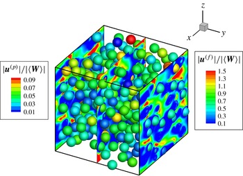
Gas–solid flows are commonly encountered in industrial devices such as fluidized beds as well as in naturally occurring phenomena such as dispersion of volcanic ash. It is clear from visual observation, experimental measurements and also from particle-resolved direct numerical simulations (PR-DNS) that the solid particles in a typical gas–solid flow have a distribution of velocities (see figure 1). Typically the particle velocity distribution is characterized by the mean velocity and the particle velocity covariance.
Particle velocity fluctuations in granular gases are characterized by the particle granular temperature, which is defined as
 $T=\left\langle \boldsymbol{v}^{\prime \prime }\boldsymbol{\cdot }\boldsymbol{v}^{\prime \prime }\right\rangle /3$
, where
 $\boldsymbol{v}^{\prime \prime }=\boldsymbol{v}-\left\langle \boldsymbol{v}\right\rangle$
denotes the fluctuation in the particle velocity
 $\boldsymbol{v}$
with respect to the mean particle velocity
 $\left\langle \boldsymbol{v}\right\rangle$
. Here angle brackets represent the average over the one-particle density that appears in the classical kinetic theory (Liboff Reference Liboff2003). In the kinetic theory of granular gases the magnitude of the particle granular temperature (relative to the square of the mean particle velocity) characterizes the importance of collisions and it is an important variable that affects transport coefficients such as viscosity and heat flux. However, many researchers (Février, Simonin & Squires Reference Février, Simonin and Squires2005) have pointed out that particle velocity fluctuations in gas–solid flows arise from both interparticle collisions as well as particle–fluid interaction. Therefore, while one may use the term particle granular temperature to refer to the trace of the particle velocity-covariance tensor, it should not be interpreted as the collisional contribution that affects transport coefficients in kinetic theory models of the particle phase. For convenience we use the term particle granular temperature to refer to the trace of the particle velocity-covariance tensor in this work, but we do not imply this to connote its usage in the kinetic theory of granular flow.
Particle velocity fluctuations play an important role in the onset of complex phenomena such as the core-annular structure observed in circulating fluidized bed risers (Gidaspow Reference Gidaspow1994). A fundamental understanding of the generation of these particle velocity fluctuations and their effect on the dynamics of gas–solid flow is necessary to develop predictive models that can capture important features of gas–solid flow behaviour such as core-annular flow.
Such studies are especially relevant due to increasing interest in carbon-neutral energy generation technologies such as chemical looping combustion (Shen et al. Reference Shen, Zheng, Xiao and Xiao2008) and fast pyrolysis of biomass (Zhang et al. Reference Zhang, Yang, Jiang, Liu and Ding2013). Gas–solid flow in such industrial devices are simulated using computational fluid dynamics (CFD) codes that are based on averaged equations for momentum and energy balance that require accurate models for terms involving interphase exchanges. For instance, the particle mean-momentum equation requires a model for the average acceleration experienced by a particle. The average particle acceleration arising from hydrodynamic forces is modelled using a drag law, which is often obtained from studies of fixed particle assemblies (Hill, Koch & Ladd Reference Hill, Koch and Ladd2001a ,Reference Hill, Koch and Ladd b ; van der Hoef, Beetstra & Kuipers Reference van der Hoef, Beetstra and Kuipers2005; Beetstra, van der Hoef & Kuipers Reference Beetstra, van der Hoef and Kuipers2007; Yin & Sundaresan Reference Yin and Sundaresan2009a ,Reference Yin and Sundaresan b ; Holloway, Yin & Sundaresan Reference Holloway, Yin and Sundaresan2010; Tenneti, Garg & Subramaniam Reference Tenneti, Garg and Subramaniam2011). However, it is also known that particle velocity fluctuations affect the fluctuating part of the drag force experienced by particles (Tenneti et al. Reference Tenneti, Garg, Hrenya, Fox and Subramaniam2010; Garzó et al. Reference Garzó, Tenneti, Subramaniam and Hrenya2012). And in turn, these fluctuations in the particle acceleration affect the evolution of the granular temperature through the acceleration–velocity correlation. The acceleration–velocity covariance arising from purely hydrodynamic effects can contribute to the generation of particle velocity fluctuations. Due to this strong coupling between particle velocity and particle acceleration, an accurate model for the particle acceleration arising from hydrodynamic forces is crucial for obtaining the correct evolution of the particle granular temperature. Hrenya & Sinclair (Reference Hrenya and Sinclair1997) show that it is necessary to capture the evolution of the particle granular temperature correctly to predict the core-annular structure observed in riser flows. Therefore, a particle acceleration model that accounts for the strong coupling between particle acceleration and particle velocity, and that can accurately predict the particle granular temperature, is needed for the successful development of gas–solid CFD simulations.
Snapshot of the flow fields in a homogeneous gas–solid flow obtained from PR-DNS of a freely-evolving gas–solid suspension corresponding to a solid volume fraction of 0.2, mean-slip Reynolds number of 20 and solid-to-fluid density ratio of 1000. Particles are coloured by the magnitude of their velocity, while the fluid is coloured by the magnitude of the fluid velocity.

The generation of particle velocity fluctuations and their effect on the dynamics of gas–solid flow has been examined from theory (Koch Reference Koch1990; Xu & Subramaniam Reference Xu and Subramaniam2007; Garzó et al. Reference Garzó, Tenneti, Subramaniam and Hrenya2012), simulations (Koch & Sangani Reference Koch and Sangani1999; Mehrabadi et al. Reference Mehrabadi, Tenneti, Garg and Subramaniam2015) and experiment (Cocco et al. Reference Cocco, Shaffer, Hays, Reddy Karri and Knowlton2010). Xu & Subramaniam (Reference Xu and Subramaniam2007) proposed the principle of conservation of interphase turbulent kinetic-energy transfer in homogeneous gas–solid suspensions. They showed that the rate of work done by the mean pressure gradient in maintaining the mean slip velocity between the gas and particle phases is responsible for the generation of fluctuations in both gas and particle velocities. PR-DNS verifies this principle in both statistically homogeneous fixed beds and freely-evolving gas–solid suspensions (Mehrabadi et al. Reference Mehrabadi, Tenneti, Garg and Subramaniam2015).
In statistically homogeneous suspensions (for a precise description see § 2.1) undergoing elastic collisions, the evolution of particle granular temperature is governed solely by the correlation of the fluctuations in particle acceleration with the fluctuations in particle velocity. In the Stokes flow regime, Koch and coworkers (Koch Reference Koch1990; Koch & Sangani Reference Koch and Sangani1999) showed that hydrodynamic forces give rise to both source and dissipation of particle granular temperature. They quantified the hydrodynamic source and dissipation of the particle granular temperature using a combination of kinetic theory closure and multipole expansion simulations at very low Reynolds numbers. Collisions cannot increase the energy in particle velocity fluctuations, so the source term in the granular temperature equation due to collisions is always zero. Inelastic collisions result in a dissipation of granular temperature, but this term is zero for elastic collisions.
When the mean slip velocity between the gas and particles corresponds to a Reynolds number outside the Stokes regime, analytical treatments are difficult but PR-DNS can be used to quantify and model the particle granular temperature. PR-DNS solves for the dynamics of particles arising from both hydrodynamic and collisional forces. The hydrodynamic force on each particle is calculated from the velocity and pressure fields that obey the Navier–Stokes equations and satisfy no slip and no-penetration boundary conditions on each particle surface, while the collisional forces are obtained from a soft-sphere collision model. Since the hydrodynamic forces on each particle are computed from a solution to the Navier–Stokes equations, PR-DNS can be considered a ‘model-free’ simulation approach when compared to other simulation methods that assume a model for the hydrodynamic force.
A widely used simple model for the instantaneous Lagrangian particle acceleration is of the form
 $\boldsymbol{A}={\it\beta}(\langle \boldsymbol{u}^{(f)}\rangle -\boldsymbol{v})$
, where
 $\boldsymbol{A}$
is the instantaneous Lagrangian particle acceleration,
 $\left\langle \boldsymbol{u}\right\rangle ^{(f)}$
is the mean fluid velocity,
 $\boldsymbol{v}$
is the instantaneous particle velocity and
 ${\it\beta}$
is the inverse time scale corresponding to the average drag experienced by the particles. The angle brackets represent averaging over the ensemble of velocity fields corresponding to a constant mean pressure gradient imposed on a statistically-homogeneous particle configuration corresponding to a specified average solid volume fraction. This model is obtained from the class of models for the mean acceleration
 $\left\langle \boldsymbol{A}\right\rangle$
formulated as
 $\left\langle \boldsymbol{A}\right\rangle ={\it\beta}(\langle \boldsymbol{u}^{(f)}\rangle -\left\langle \boldsymbol{v}\right\rangle )$
, by replacing the mean particle velocity
 $\left\langle \boldsymbol{v}\right\rangle$
with its instantaneous counterpart. Such models are widely used in gas–solid CFD simulations based on a Lagrangian particle representation coupled with an Eulerian gas-phase representation that is employed in codes such as MFIX-DEM (Garg et al.
Reference Garg, Galvin, Li and Pannala2010). This class of Lagrangian models for the particle acceleration due to hydrodynamic forces produces only a dissipation term in the granular temperature evolution equation, and no source term. Consequently, they are unable to predict the steady granular temperature that is observed in PR-DNS of statistically homogeneous gas–solid suspensions over a range of Reynolds number and solid volume fraction values. Note that the failure of this class of Lagrangian models for the particle acceleration due to hydrodynamic forces is independent of the collision model because collisions cannot be a source of granular temperature.
The inadequacy of simple extensions to the mean drag model in accurately describing the physics in a gas–solid suspension can be understood by considering an isolated sphere in a fluid. The motion of a rigid isolated sphere can be described accurately by the Maxey–Riley equation (Maxey & Riley Reference Maxey and Riley1983). Usually for high solid-to-fluid density ratio
 ${\it\rho}_{p}/{\it\rho}_{f}\sim O(10^{3})$
, steady drag dominates. However, Faxén corrections (Calzavarini et al.
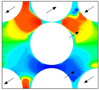
Reference Calzavarini, Volk, Bourgoin, Lévêque, Pinton and Toschi2009; Homann & Bec Reference Homann and Bec2010) may not be negligible for finite size particles if the velocity gradients are high. In suspensions, neighbouring particles affect the local flow, strain rate and also the pressure (see figure 2) and can cause the fluid velocity to change over length scales that are much smaller than the particle diameter. Therefore, considering only the steady drag to model the particle acceleration may not be sufficient in gas–solid suspensions.
Pressure contours obtained from the PR-DNS of a gas–solid suspension corresponding to a solid volume fraction of 0.2 and a mean slip Reynolds number of 20. Arrows in the figure indicate the directions of the velocities of the particles. The figure shows how the pressure field on a particle is modified due to the presence of neighbouring particles. Reproduced from Garzó et al. (Reference Garzó, Tenneti, Subramaniam and Hrenya2012).

Tenneti et al. (Reference Tenneti, Garg, Hrenya, Fox and Subramaniam2010) used PR-DNS to quantify the effect of particle velocity fluctuations on the fluctuating part of the hydrodynamic force experienced by the particles. Recent findings by Tenneti et al. (Reference Tenneti, Garg, Hrenya, Fox and Subramaniam2010) and Garzó et al. (Reference Garzó, Tenneti, Subramaniam and Hrenya2012), indicate that the particle acceleration has a stochastic contribution due to its interaction with neighbouring particles. In order to account for the stochastic nature of the neighbour particle effects, Garzó et al. (Reference Garzó, Tenneti, Subramaniam and Hrenya2012) proposed a Langevin type equation to model the Lagrangian particle acceleration in the Stokes flow regime. A Langevin model for the increment in particle velocity results in a closed Fokker–Planck equation for the one-particle distribution function, and Garzó et al. (Reference Garzó, Tenneti, Subramaniam and Hrenya2012) derived the transport coefficients in the moment equations that follow from the Fokker–Planck equation.
In this work we consider the problem of extending the Lagrangian model for particle acceleration due to hydrodynamic forces to flows corresponding to moderate Reynolds number based on the slip velocity between gas and particles. These are relevant to simulation approaches based on a Lagrangian description of the solid particles that interact with an Eulerian description of the gas phase. This Lagrangian–Eulerian (LE) approach (Subramaniam Reference Subramaniam2013) is common to a variety of mathematical representations and models for gas–solid flow, including the PR-DNS approach that is used in this work. However, the LE approach can be used to also solve for a filtered representation of the fluid velocity field in conjunction with a discrete element method for the particles (LES-DEM) (Capecelatro, Desjardins & Fox Reference Capecelatro, Desjardins and Fox2014), or an averaged equation representation of the fluid velocity field (as in the Eulerian two-fluid model) coupled with DEM representation of the particles resulting in a CFD-DEM approach such as MFIX-DEM (Garg et al. Reference Garg, Galvin, Li and Pannala2010). In the LES-DEM and CFD-DEM approaches, the acceleration of each particle needs to be modelled, given its velocity and position and available statistics of the fluid flow field. Since current models for particle acceleration based on the steady average-drag law are clearly inadequate, there is a need for a better class of particle acceleration models for gas–solid flows, which result in a granular temperature equation with proper representation of the physics that lead to source and dissipation of particle granular temperature. Although the specific form of such a model when adapted to each LE method may vary in terms of the model coefficients, the development of the modelling framework will find general applicability.
A key finding from the work of Garzó et al. (Reference Garzó, Tenneti, Subramaniam and Hrenya2012) is that in order to properly address this modelling problem it is necessary to begin with the evolution equation of the one-particle distribution function (that contains the particle velocity distribution), rather than the mean and second-moment equations that follow from it. The present work uses PR-DNS to extend the Langevin model proposed by Garzó et al. (Reference Garzó, Tenneti, Subramaniam and Hrenya2012) to moderate mean-slip Reynolds numbers. Such a Lagrangian modelling framework for particle acceleration due to hydrodynamic forces can be useful in various LE approaches such as LES-DEM or CFD-DEM described earlier, where it can be coupled with soft sphere or hard-sphere collision models, although the model coefficients will be specific to the approach. If we consider the Eulerian two-fluid model of gas–solid flow, then the particle velocity statistics are closed at the level of the granular temperature. Since the Lagrangian particle acceleration model implies models for the source and dissipation terms arising from hydrodynamic forces in the granular temperature equation, it implies a closure for those terms in the granular temperature equation in the Eulerian two-fluid model as well.
In this work, we use the one-particle distribution function as a starting point to understand the mechanism of generation of particle velocity fluctuations in statistically homogeneous gas–solid flows undergoing elastic collisions at moderate Reynolds numbers based on the mean slip velocity between the gas and the solid phases. We use PR-DNS of freely-evolving gas–solid suspensions at moderate Reynolds numbers to quantify the hydrodynamic source and dissipation of granular temperature at moderate Reynolds numbers. We also use PR-DNS to propose a stochastic Lagrangian model for the hydrodynamic particle acceleration that captures the correct evolution of the particle granular temperature.
The rest of the paper is organized as follows. The theoretical background to the source and dissipation of granular temperature is presented first. The numerical method used in the PR-DNS is described along with validation results. PR-DNS results quantifying the source and dissipation of the granular temperature arising from particle acceleration due to hydrodynamic forces at moderate Reynolds numbers are presented next. This is followed by the details of the Lagrangian model for particle acceleration due to hydrodynamic forces that has the capability of capturing the strong coupling between particle acceleration and the particle velocity distribution. The Langevin form of the particle acceleration model is verified by comparing with PR-DNS data. Then the specification of the model coefficients in terms of solid volume fraction, mean-flow Reynolds number, solid-to-fluid density ratio and particle granular temperature are described. The Lagrangian particle acceleration model is then tested using a CFD-DEM simulation where it is coupled to a soft-sphere model for collisional interactions and compared with PR-DNS results. This is followed by a discussion of the model assumptions and limitations and finally conclusions are summarized.
2. Theory
In any statistical closure problem an important modelling question is the adequacy of the mathematical representation to capture physical phenomena. The work of Hrenya & Sinclair (Reference Hrenya and Sinclair1997) shows that closure only at the level of the mean momentum is not adequate to capture the profiles of mean solid volume fraction and mean particle velocity in core-annular flow, but a closure at the level of the second moment of particle velocities is necessary. The starting point in this work for understanding the generation of particle velocity fluctuations is to consider the evolution of the one-particle distribution function, also referred to as the number density function (NDF).
We consider monodisperse particles moving in a gas under the influence of both hydrodynamic and collisional forces. We consider the one-particle distribution function
 $f(\boldsymbol{x},\boldsymbol{v},t)$
that is the density of the average number of particles
 $\langle N\rangle$
in
 $(\boldsymbol{x},\boldsymbol{v})$
space, such that
 $\int f(\boldsymbol{x},\boldsymbol{v},t)\,\text{d}\boldsymbol{x}\,\text{d}\boldsymbol{v}=\langle N\rangle$
. If the system is examined on time scales smaller than the duration of each collision (as is the case for the soft-sphere collision model used in the PR-DNS), then the corresponding evolution equation for the one-particle distribution function
 $f(\boldsymbol{x},\boldsymbol{v},t)$
is given by (Subramaniam Reference Subramaniam2001; Liboff Reference Liboff2003)
 $$\begin{eqnarray}\frac{\partial f}{\partial t}+\boldsymbol{{\rm\nabla}}_{\boldsymbol{x}}\boldsymbol{\cdot }\left(\boldsymbol{v}f\right)+\boldsymbol{{\rm\nabla}}_{\boldsymbol{v}}\boldsymbol{\cdot }\{(\left\langle \boldsymbol{A}_{h}\mid \boldsymbol{x},\boldsymbol{v};t\right\rangle +\left\langle \boldsymbol{A}_{c}\mid \boldsymbol{x},\boldsymbol{v};t\right\rangle )f\}=0,\end{eqnarray}$$
where the conditional average of the particle acceleration
 $\left\langle \boldsymbol{A}\mid \boldsymbol{x},\boldsymbol{v};t\right\rangle =\left\langle \boldsymbol{A}_{h}\mid \boldsymbol{x},\boldsymbol{v};t\right\rangle +\left\langle \boldsymbol{A}_{c}\mid \boldsymbol{x},\boldsymbol{v};t\right\rangle$
has been decomposed into contributions arising from both hydrodynamic
 $\left\langle \boldsymbol{A}_{h}\mid \boldsymbol{x},\boldsymbol{v};t\right\rangle$
and collisional forces
 $\left\langle \boldsymbol{A}_{c}\mid \boldsymbol{x},\boldsymbol{v};t\right\rangle$
. If a soft-sphere collision model is considered then each collision occurs over a finite time interval, and this is the case for the PR-DNS computations where the duration of each soft-sphere collision is fully resolved. The PR-DNS results presented later in the paper correspond to this soft-sphere NDF equation (2.1).
If a mesoscale time averaging is performed over a time scale that is larger than the duration of each collisional contact, but smaller than the time between collisions, then collision events can be modelled as binary and instantaneous. This leads to the Boltzmann model for a dilute system of hard spheres immersed in a fluid (or the Boltzmann–Enskog model for higher particle solid volume fraction). Note that in these hard sphere models, only the change in impulse can be defined for an instantaneous collision, whereas in the soft-sphere model the particle acceleration due to collision can be meaningfully defined. We now examine the Boltzmann–Enskog transport equation for the one-particle distribution function in gas–solid flow.
For monodisperse particles undergoing binary, instantaneous collisions in a fluid, the one-particle distribution function
 $f(\boldsymbol{x},\boldsymbol{v},t)$
is defined in a position–velocity space (Williams Reference Williams1958; Koch Reference Koch1990; Subramaniam Reference Subramaniam2000, Reference Subramaniam2013; Liboff Reference Liboff2003; Garzo, Dufty & Hrenya Reference Garzo, Dufty and Hrenya2007; Marchisio & Fox Reference Marchisio and Fox2013), and evolves by the following transport equation:
 $$\begin{eqnarray}\frac{\partial f}{\partial t}+\boldsymbol{{\rm\nabla}}_{\boldsymbol{x}}\boldsymbol{\cdot }\left(\boldsymbol{v}f\right)+\boldsymbol{{\rm\nabla}}_{\boldsymbol{v}}\boldsymbol{\cdot }\left(\left\langle \tilde{\boldsymbol{A}}_{h}\mid \boldsymbol{x},\boldsymbol{v};t\right\rangle f\right)={\dot{f}}_{\mathit{coll}},\end{eqnarray}$$
where
 $\boldsymbol{{\rm\nabla}}_{\boldsymbol{x}}$
and
 $\boldsymbol{{\rm\nabla}}_{\boldsymbol{v}}$
denote the gradient operators in the position–velocity space, respectively,
 $\langle \tilde{\boldsymbol{A}}_{h}\mid \boldsymbol{x},\boldsymbol{v};t\rangle$
is the mesoscale conditional average of the particle acceleration due to hydrodynamic forces, and
 ${\dot{f}}_{\mathit{coll}}$
is the collisional term that depends on the two-particle density. (Angle brackets here represent averaging over the two-particle density in the kinetic theory of gas–solid flow (Koch Reference Koch1990).) The mesoscale conditional average of the particle acceleration due to hydrodynamic forces
 $\langle \tilde{\boldsymbol{A}}_{h}\mid \boldsymbol{x},\boldsymbol{v};t\rangle$
in this equation is the mesoscale time-averaged counterpart of the corresponding term in (2.1), but because the hydrodynamic fields change negligibly over the duration of a collision, as a first approximation they can be taken to be identical. So from this point we drop the tilde that distinguishes this quantity between the two equations. A closure model for the collisional term results in a kinetic equation. This well-known equation has been extensively studied in the context of granular flows where collisions are inelastic. Extensions to non-dilute cases that follow the Enskog approach have also been pursued.
The principal difference between the kinetic theory of molecular (or granular) gases and the kinetic theory of gas–solid flow is that in the latter, the conditional particle acceleration due to the hydrodynamic force
 $\left\langle \boldsymbol{A}_{h}\mid \boldsymbol{x},\boldsymbol{v};t\right\rangle$
depends on the particle velocity through slip with respect to the fluid, and hence is retained inside the velocity derivative in the velocity transport term. This conditional particle acceleration is caused by the hydrodynamic force
 $\boldsymbol{F}_{\mathit{fluid}}=m\left\langle \boldsymbol{A}_{h}\mid \boldsymbol{x},\boldsymbol{v};t\right\rangle$
experienced by the particle due to the pressure and velocity gradient fields at the particle surface. In the transport equation for the distribution function (cf. (2.2)),
 $\langle \boldsymbol{A}_{h}\mid \boldsymbol{x},\boldsymbol{v};t\rangle$
depends on the instantaneous particle velocity
 $\boldsymbol{v}$
and can vary in both space and time. For the spatially homogeneous case with monodisperse particles it can be interpreted as the average acceleration experienced by a particle with velocity
 $\boldsymbol{v}$
. The averaging operator
 $\langle \cdot \rangle$
represents integration over all higher-order multiparticle distribution functions (Koch Reference Koch1990; Subramaniam Reference Subramaniam2000) that can be defined on the basis of the ensemble of particles with position and velocity
 $\{\boldsymbol{X}^{(n)}(t),\boldsymbol{V}^{(n)}(t),n=1,\ldots ,N\}$
. In particular, the conditional acceleration
 $\langle \boldsymbol{A}_{h}\mid \boldsymbol{x},\boldsymbol{v};t\rangle$
is obtained by integrating out its dependence on the two-particle density (pair correlation function). In other words, the conditional acceleration
 $\langle \boldsymbol{A}_{h}\mid \boldsymbol{x},\boldsymbol{v};t\rangle$
is not completely determined by the particle velocity, but may be affected by the presence of neighbour particles.
Returning to (2.1) that applies to time-resolved collisions as in the PR-DNS, for simplicity we denote the conditional acceleration term
 $\left\langle \boldsymbol{A}\mid \boldsymbol{x},\boldsymbol{v};t\right\rangle$
representing both hydrodynamic and collisional effects as
 $\boldsymbol{A}$
in the rest of the paper. An important observation is that a model for
 $\boldsymbol{A}$
implies a model for the mean interphase momentum transfer as well as a model for the source and dissipation of granular temperature. Note that if we write
 $\boldsymbol{A}=\left\langle \boldsymbol{A}\right\rangle +\boldsymbol{A}^{\prime \prime }$
, then
 $\left\langle \boldsymbol{A}\right\rangle$
represents the mean interphase momentum transfer (drag) that has been studied extensively, as noted earlier. Since collisions conserve linear momentum, the collisional contribution to mean interphase momentum transfer is zero. The focus of this paper is to develop a model for the fluctuating particle acceleration that closes the evolution equation of particle granular temperature. We now discuss the evolution of particle granular temperature and identify the source and dissipation terms in statistically homogeneous gas–solid flows.
2.1. Source and dissipation of particle granular temperature
The averaged equations for mean momentum conservation and transport of the second moment of particle velocity implied by (2.1) are derived using the usual procedure to derive moment equations from the density evolution equation (2.1) (Pai & Subramaniam Reference Pai and Subramaniam2009; Subramaniam Reference Subramaniam2013). Statistical homogeneity in the context of gas–solid flows implies that the one-particle distribution function
 $f$
and the single-point probability density function of fluid velocity are both independent of the spatial coordinate
 $\boldsymbol{x}$
. Such particle fields can be represented by particle configurations that maintain a spatially-uniform solid volume fraction and spatially-uniform velocity statistics such as mean particle velocity and granular temperature. In the PR-DNS, these initial particle configurations are generated by elastically colliding particles that have been initialized with a specified uniform solid volume fraction in a periodic box. This ensures that all the configurations have the same initial two-point statistics such as the pair correlation function, and for elastic collisions we see that this pair correlation does not change in time. The fluid velocity field also has spatially-uniform velocity statistics such as mean fluid velocity and covariance at steady state (Mehrabadi et al.
Reference Mehrabadi, Tenneti, Garg and Subramaniam2015). For the simple case of statistically homogeneous gas–solid flow undergoing elastic collisions, the second moment of the particle fluctuating velocity evolves as:
 $$\begin{eqnarray}\frac{\text{d}}{\text{d}t}\left\langle v_{i}^{\prime \prime }v_{j}^{\prime \prime }\right\rangle =\left\langle A_{i}^{\prime \prime }v_{j}^{\prime \prime }\right\rangle +\left\langle A_{j}^{\prime \prime }v_{i}^{\prime \prime }\right\rangle \!.\end{eqnarray}$$
Here
 $\boldsymbol{A}^{\prime \prime }$
denotes the fluctuation in the conditional particle acceleration arising from both hydrodynamic and collisional forces. By taking the trace of (2.3) and dividing throughout by three, we obtain the evolution of the particle granular temperature as:
 $$\begin{eqnarray}\frac{\text{d}T}{\text{d}t}=\frac{2}{3}\left\langle A_{i}^{\prime \prime }v_{i}^{\prime \prime }\right\rangle =S-{\it\Gamma},\end{eqnarray}$$
where
 $S$
and
 ${\it\Gamma}$
represent the decomposition of the right-hand side into source and dissipation terms, as proposed earlier by Koch (Reference Koch1990). The trace of the tensor
 $\langle A_{i}^{\prime \prime }v_{j}^{\prime \prime }\rangle$
that appears on the right-hand side of (2.4) can be positive or negative. In a statistically homogeneous gas–solid flow with a constant mean pressure gradient, the granular temperature reaches a steady value. Depending on the initial conditions, this term can act as a sink (for initial granular temperature higher than the steady value) or as a source (for initial granular temperature lower than the steady value). Koch and coworkers (Koch Reference Koch1990; Koch & Sangani Reference Koch and Sangani1999) proposed a decomposition of
 $\left\langle A_{i}^{\prime \prime }v_{i}^{\prime \prime }\right\rangle$
into source and sink terms and provided expressions for these terms in Stokes flow.
Here we follow an approach similar to that of Koch that leads to new results relevant to suspensions at moderate Reynolds number. If we decompose the fluctuation in the conditional particle acceleration
 $\boldsymbol{A}^{\prime \prime }$
into hydrodynamic and collisional contributions as in (2.1), we can rewrite (2.4) as
 $$\begin{eqnarray}\frac{\text{d}T}{\text{d}t}=\frac{2}{3}\left(\left\langle A_{h,i}^{\prime \prime }v_{i}^{\prime \prime }\right\rangle +\left\langle A_{c,i}^{\prime \prime }v_{i}^{\prime \prime }\right\rangle \right)=(S_{h}-{\it\Gamma}_{h})+(S_{c}-{\it\Gamma}_{c}).\end{eqnarray}$$
Since collisions do not generate energy in particle velocity fluctuations the source term
 $S_{c}=0$
. Inelastic collisions result in a dissipation of granular temperature, but for elastic collisions the dissipation of energy
 ${\it\Gamma}_{c}=0$
. Therefore, we have a simpler equation for the granular temperature evolution in elastically colliding gas–solid suspensions:
 $$\begin{eqnarray}\frac{\text{d}T}{\text{d}t}=\frac{2}{3}\left(\left\langle A_{h,i}^{\prime \prime }v_{i}^{\prime \prime }\right\rangle +\left\langle A_{c,i}^{\prime \prime }v_{i}^{\prime \prime }\right\rangle \right)=S_{h}-{\it\Gamma}_{h},\end{eqnarray}$$
where the source and sink terms in the granular temperature equation arise solely from particle acceleration due to hydrodynamic forces. Collisions may still contribute to the redistribution of energy in the various components of the particle velocity-covariance tensor and the evolution of its anisotropy are discussed in Garzó et al. (Reference Garzó, Tenneti, Subramaniam and Hrenya2012). An interesting observation regarding particle acceleration models based on a simple extension of the mean drag law is that they only contribute to the dissipation
 ${\it\Gamma}_{h}$
in (2.6) and the source term
 $S_{h}$
is zero (details in appendix A). Hence, they predict a granular temperature equation that always decays to zero for all mean slip Reynolds number values irrespective of the collision model, which is unphysical and not observed in PR-DNS.
In general the decomposition of
 $\left\langle A_{i}^{\prime \prime }v_{i}^{\prime \prime }\right\rangle$
into source and dissipation terms shown in (2.4) is non-unique. Here we demonstrate a simple way to extract these source and sink terms for the case of a statistically homogeneous suspension. The application of this method to extract the source and sink terms corresponding to the hydrodynamic contribution (
 $S_{h}$
and
 ${\it\Gamma}_{h}$
) from PR-DNS at moderate mean-slip Reynolds numbers is described in appendix B. Note that (2.3) is obtained by multiplying the one-particle density evolution equation (2.1) by
 $v_{i}^{\prime \prime }v_{j}^{\prime \prime }$
and integrating over the one-particle density. Therefore, the averaging operator
 $\left\langle \cdot \right\rangle$
in (2.3) and (2.4) represents an average over the entire velocity space, i.e. for any quantity
 $Q$
, its average
 $\left\langle Q\right\rangle$
is defined as:
 $$\begin{eqnarray}\left\langle Q\right\rangle \left(\boldsymbol{x},t\right)=\frac{1}{n\left(\boldsymbol{x},t\right)}\int _{[\boldsymbol{v}]}Qf(\boldsymbol{x},\boldsymbol{v},t)\,\text{d}\boldsymbol{v}.\end{eqnarray}$$
For statistically homogeneous flows, the particle acceleration–velocity covariance is:
 $$\begin{eqnarray}\left\langle A_{i}^{\prime \prime }v_{i}^{\prime \prime }\right\rangle =\frac{1}{n}\int _{[\boldsymbol{v}]}A_{i}^{\prime \prime }v_{i}^{\prime \prime }f(\boldsymbol{x},\boldsymbol{v},t)\,\text{d}\boldsymbol{v}.\end{eqnarray}$$
It is clear from (2.4) that in statistically homogeneous flows the granular temperature evolves solely due to the particle acceleration–velocity covariance. Therefore, this term must contain both the source and dissipation of granular temperature. In order to uniquely identify the source and sink terms, we decompose the fluctuating conditional acceleration vector into a component that is aligned with the fluctuating velocity vector
 $\boldsymbol{v}^{\prime \prime }$
and one that is perpendicular to
 $\boldsymbol{v}^{\prime \prime }$
, i.e.
 $$\begin{eqnarray}A_{i}^{\prime \prime }=-{\it\zeta}v_{i}^{\prime \prime }+A_{R,i}^{\prime \prime },\end{eqnarray}$$
where the component of the acceleration perpendicular to the fluctuating velocity is denoted
 ${A^{\prime \prime }}_{R,i}$
. Note that there are no assumptions made in performing this decomposition. From the above equation it is clear that the coefficient
 ${\it\zeta}$
can be obtained as
 ${\it\zeta}=A_{i}^{\prime \prime }v_{i}^{\prime \prime }/(v_{k}^{\prime \prime }v_{k}^{\prime \prime })$
. In fact, the sign of
 ${\it\zeta}$
tells us if the fluctuating acceleration of the particle is in the direction of the fluctuating particle velocity, or opposite to it. We can define two new variables
 ${\it\zeta}_{+}=\left({\it\zeta}+\left|{\it\zeta}\right|\right)/2$
and
 ${\it\zeta}_{-}=\left({\it\zeta}-\left|{\it\zeta}\right|\right)/2$
that are strictly positive and negative, respectively. Substituting the decomposition for the fluctuating particle acceleration in (2.8), and using the definitions of
 ${\it\zeta}_{+}$
and
 ${\it\zeta}_{-}$
, we obtain
 $$\begin{eqnarray}\left\langle A_{i}^{\prime \prime }v_{i}^{\prime \prime }\right\rangle =\frac{1}{n}\left(-\int _{[\boldsymbol{v}]}{\it\zeta}_{-}v_{i}^{\prime \prime }v_{i}^{\prime \prime }f(\boldsymbol{x},\boldsymbol{v},t)\,\text{d}\boldsymbol{v}\right)+\frac{1}{n}\left(-\int _{[\boldsymbol{v}]}{\it\zeta}_{+}v_{i}^{\prime \prime }v_{i}^{\prime \prime }f(\boldsymbol{x},\boldsymbol{v},t)\,\text{d}\boldsymbol{v}\right).\end{eqnarray}$$
Clearly, the first term on the right-hand side of the above equation is positive, and the second term is negative. Therefore, the evolution equation of the particle granular temperature can be rewritten as
 $$\begin{eqnarray}\frac{\text{d}T}{\text{d}t}=S-{\it\Gamma},\end{eqnarray}$$
where the source
 $S$
and dissipation
 ${\it\Gamma}$
of the particle granular temperature are uniquely identified as
 $$\begin{eqnarray}S={\textstyle \frac{2}{3}}\left\langle -{\it\zeta}_{-}v_{i}^{\prime \prime }v_{i}^{\prime \prime }\right\rangle \!,\end{eqnarray}$$
and
 $$\begin{eqnarray}{\it\Gamma}={\textstyle \frac{2}{3}}\left\langle {\it\zeta}_{+}v_{i}^{\prime \prime }v_{i}^{\prime \prime }\right\rangle \!.\end{eqnarray}$$
Note that in the case of elastically colliding particles there is no contribution from the collisional particle acceleration to the source and sink terms, which are wholly determined by the hydrodynamic contribution to particle acceleration. Therefore, this approach enables us to identify the source
 $S_{h}$
and sink
 ${\it\Gamma}_{h}$
terms in (2.6) from PR-DNS data that provides the hydrodynamic acceleration
 $\boldsymbol{A}_{h}$
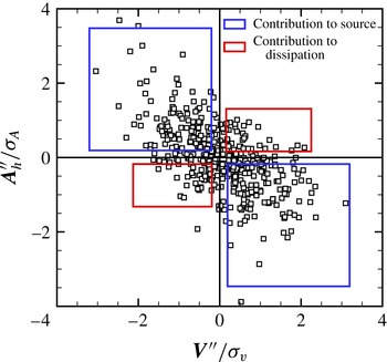
and velocity for all the particles. A key observation from this derivation is that particles with their fluctuating acceleration aligned with their fluctuating velocity contribute to the source of granular temperature. Particles with the fluctuating acceleration aligned in a direction opposite to that of the fluctuating velocity contribute to the dissipation in granular temperature. This can be easily visualized from the scatter plot shown in figure 3. For illustration, in this figure we show the scatter plot of fluctuating particle acceleration (from hydrodynamic forces) and fluctuating particle velocity obtained from the PR-DNS of flow past a freely-evolving suspension with solid volume fraction
 ${\it\phi}=0.2$
, mean-slip Reynolds number
 $\mathit{Re}_{m}=20$
and initial granular temperature corresponding to
 $\mathit{Re}_{T}=6$
(where
 $\mathit{Re}_{T}$
is defined by (6.1)). The symbols that lie in the first and the third quadrants denote the particles whose fluctuating acceleration is aligned with the fluctuating velocity. Hence, these particles contribute to the source in granular temperature.
Scatter plot showing the fluctuating particle acceleration arising from hydrodynamic forces versus the fluctuating particle velocity obtained from the PR-DNS of a freely-evolving suspension with a volume fraction of 0.1, mean-slip Reynolds number of 20 and Reynolds number based on initial granular temperature of 6. From the analysis on the extraction of source and dissipation from the PR-DNS, we can see that the symbols that lie in the first and the third quadrant contribute to source and the symbols that lie in the second and the fourth quadrant contribute to the dissipation.

The source term in the granular temperature equation plays an important role in sustaining a non-zero value for the granular temperature at steady state. In its absence the granular temperature in a homogeneous suspension would simply decay to zero, leading to an infinite Mach number in the particle phase. Not only is this problematic from a numerical standpoint for CFD simulations, but it is also unphysical over a wide range of mean-flow Reynolds number and volume fraction. So a good model for the fluctuating particle acceleration should result in an accurate prediction of acceleration–velocity covariance, which in turn results in the correct evolution of granular temperature. In § 7 we consider a stochastic model of the Langevin type, because the coefficients of such a model can be related to the source and dissipation of granular temperature using the fluctuation–dissipation theorem. We use PR-DNS of freely-evolving gas–solid suspensions at moderate Reynolds number to quantify the granular temperature and its source and dissipation at steady state. We now briefly discuss the numerical method used to perform the simulations.
3. Numerical method
In this study, PR-DNS of freely-evolving gas–solid suspensions are performed using the particle-resolved uncontaminated-fluid reconcilable immersed-boundary method (PUReIBM) that has been developed to simulate flow past fixed particle assemblies (Garg et al. Reference Garg, Tenneti, Mohd-Yusof, Subramaniam, Pannala, Syamlal and O’Brien2011) and freely-evolving suspensions (Tenneti et al. Reference Tenneti, Garg, Hrenya, Fox and Subramaniam2010). In PUReIBM, the entire physical domain is discretized using a uniform Cartesian grid and the governing equations of fluid flow are solved on all the grid points (including those lying inside the particles). The governing equations that are solved in the PUReIBM method are the continuity equation
 $$\begin{eqnarray}\boldsymbol{{\rm\nabla}}\boldsymbol{\cdot }\boldsymbol{u}=0,\end{eqnarray}$$
and the Navier–Stokes equations
 $$\begin{eqnarray}{\it\rho}_{f}\frac{\partial \boldsymbol{u}}{\partial t}+{\it\rho}_{f}\boldsymbol{{\rm\nabla}}\boldsymbol{\cdot }\left(\boldsymbol{u}\boldsymbol{u}\right)=-\boldsymbol{g}_{\mathit{IBM}}+{\it\mu}_{f}{\rm\nabla}^{2}\boldsymbol{u}+\boldsymbol{f}-{\it\rho}_{f}\boldsymbol{A}_{f}.\end{eqnarray}$$
Here
 $\boldsymbol{u}$
is the instantaneous velocity field and
 $\boldsymbol{g}_{\mathit{IBM}}$
is the pressure gradient. The third term on the right-hand side of (3.2) is the immersed boundary (IB) force
 $\boldsymbol{f}$
that accounts for the presence of solid particles by ensuring the no slip and no-penetration boundary conditions at the surface of the particles. The final term on the right-hand side of (3.2) is the force per unit volume due to acceleration
 $\boldsymbol{A}_{f}$
of the reference frame. The governing equations in PUReIBM are formulated in an accelerating frame of reference that moves with the mean velocity of the particles. This formulation enables the simulation of not only sedimenting suspensions, but also suspensions with arbitrary values of mean slip velocity, while maintaining average particle motion at rest in the accelerating frame motion. The full details of the formulation in an accelerating frame of reference are given in the work of Tenneti et al. (Reference Tenneti, Garg, Hrenya, Fox and Subramaniam2010).
As described earlier, the IB force
 $\boldsymbol{f}$
in (3.2) is used to impose the no slip and no-penetration conditions on the fluid velocity at the fluid–particle interface. Complete details of the computation of the IB force can be found in the work of Tenneti et al. (Reference Tenneti, Garg and Subramaniam2011). The surface of the spherical particle is represented by a discrete number of points, called boundary points, that are parametrized in spherical coordinates. Two additional sets of points, termed the exterior and interior points are generated by projecting the boundary points onto spheres of radii
 $r+{\rm\Delta}r$
and
 $r-{\rm\Delta}r$
respectively, with
 ${\rm\Delta}r$
chosen to be equal to the grid spacing. In PUReIBM, the IB force is computed at the interior points so that a desired velocity
 $\boldsymbol{u}^{(d,k)}$
is obtained at the
 $k$
th interior point. Following the direct forcing method proposed by Yusof (Reference Yusof1996) the IB force
 $\boldsymbol{f}^{(k)}$
at the
 $k$
th interior point is computed as:
 $$\begin{eqnarray}\boldsymbol{f}^{(k)}={\it\rho}_{f}\frac{\boldsymbol{u}^{(k,d)}-\boldsymbol{u}^{(k,n)}}{{\rm\Delta}t}+{\it\rho}_{f}\boldsymbol{S}^{(k,n)}+\boldsymbol{g}_{\mathit{IBM}}^{(k,n)}-{\it\mu}_{f}{\rm\nabla}^{2}\boldsymbol{u}^{(k,n)}+{\it\rho}^{(f)}\boldsymbol{A}_{f}.\end{eqnarray}$$
In the above expression,
 $\boldsymbol{S}^{(k,n)}$
is the convective term evaluated at the
 $k$
th interior point. When the expression for the IB force given in (3.3) is substituted in the discretized version of (3.2), the velocity at the
 $k$
th interior point is forced to the desired value
 $\boldsymbol{u}^{(k,d)}$
. Note that all the terms in the above equation are evaluated at the
 $k$
th interior point. The desired velocity
 $\boldsymbol{u}^{(k,d)}$
depends on the velocity of the particle. For instance, for a fixed particle the desired velocity at the interior point is equal in magnitude but opposite in direction of the fluid velocity at the corresponding exterior point so that the velocity at the boundary point is zero. The IB force so computed at all the interior points is interpolated to the neighbouring grid nodes that do not include those lying in the fluid phase to get
 $\boldsymbol{f}$
.
It has been shown by Tenneti et al. (Reference Tenneti, Garg and Subramaniam2011) that volume-averaged equations in a periodic domain can be reconciled with the ensemble-averaged equations of statistically homogeneous gas–solid suspensions. Hence the governing equations (3.1) and (3.2) are solved numerically in a cubic domain with periodic boundaries, since the primary goal is to simulate statistically-homogeneous suspensions. Similar to DNS of single-phase turbulence, it is simpler to solve for appropriately defined fluctuating variables. The velocity field is decomposed into a spatially uniform mean flow
 $\left\langle \boldsymbol{u}\right\rangle _{\mathscr{V}}\left(t\right)$
and a fluctuating velocity field
 $\boldsymbol{u}^{\prime }$
, i.e.
 $$\begin{eqnarray}\boldsymbol{u}\left(\boldsymbol{x},t\right)=\left\langle \boldsymbol{u}\right\rangle _{\mathscr{V}}\left(t\right)+\boldsymbol{u}^{\prime }\left(\boldsymbol{x},t\right)\!,\end{eqnarray}$$
where the volumetric mean velocity is obtained by averaging the velocity field over the entire computational domain. Similar decompositions are written for the convective term, the pressure gradient
 $\boldsymbol{g}_{IBM}$
and IB force. Substituting the above decompositions in (3.1) and (3.2), followed by averaging over the entire computational domain, yields the volume-averaged mass and momentum conservation equations (detailed equations are given by Tenneti et al. (Reference Tenneti, Garg and Subramaniam2011)). Evolution equations for the fluctuating variables are derived by subtracting the volume-averaged equations from their instantaneous counterparts. The resulting equations for the fluctuating variables are solved using a pseudo-spectral method, with the Crank–Nicolson scheme for the viscous terms and an Adams–Bashforth scheme for the convective terms. A fractional time-stepping method that is based on Kim and Moin’s approach (Kim & Moin Reference Kim and Moin1985) is used to advance the fluctuating velocity fields in time.
In freely-evolving gas–solid suspensions, the particles move under the influence of hydrodynamic and collisional forces. In PUReIBM, the particles are represented in a Lagrangian frame of reference. The position and translational velocity of the
 $i$
th particle at time
 $t$
are denoted
 $\boldsymbol{X}^{(i)}(t)$
and
 $\boldsymbol{V}^{(i)}(t)$
, respectively, and they evolve in time as:
 $$\begin{eqnarray}\displaystyle & \displaystyle \frac{\text{d}\boldsymbol{X}^{(i)}(t)}{\text{d}t}=\boldsymbol{V}^{(i)}(t), & \displaystyle\end{eqnarray}$$
 $$\begin{eqnarray}\displaystyle & \displaystyle m\frac{\text{d}\boldsymbol{V}^{(i)}(t)}{\text{d}t}=\boldsymbol{B}+\boldsymbol{F}_{h}^{(i)}(t)+\mathop{\sum }_{\substack{ j=1 \\ j\neq i}}^{N_{p}}\boldsymbol{F}_{ij}^{(c)}(t), & \displaystyle\end{eqnarray}$$
 $\boldsymbol{B}$
is any external body force,
 $\boldsymbol{F}_{h}^{(i)}$
is the hydrodynamic force (calculated from the velocity and pressure fields at the particle surface) and
 $\boldsymbol{F}_{ij}^{(c)}$
is the contact force on the
 $i$
th particle as a result of collision with
 $j$
th particle. Here
 $N_{p}$
is the total number of particles used in the simulation. Particle collisions are treated using a soft-sphere model originally proposed by Cundall & Strack (Reference Cundall and Strack1979). In the soft-sphere approach, particles are allowed to overlap during a collision, and the contact mechanics between the overlapping particles is modelled by a system of springs and dashpots in both normal and tangential directions. The spring causes the colliding particles to rebound, and the dashpot mimics the dissipation of kinetic energy due to inelastic collisions. The spring stiffness coefficients in the tangential and normal directions are
 $k_{t}$
and
 $k_{n}$
, respectively. Similarly, the dashpot damping coefficients in the tangential and normal directions are
 ${\it\eta}_{t}$
and
 ${\it\eta}_{n}$
, respectively. The spring stiffness and dashpot damping coefficients are related to the coefficient of restitution and the coefficient of friction (Garg et al.
Reference Garg, Galvin, Li and Pannala2010).
The particles considered in this study are assumed to be frictionless. This implies that the tangential component of the contact force is zero, and thus rotation of particles is not accounted for in this study. Therefore, only the normal component of the contact force
 $\boldsymbol{F}_{\boldsymbol{n}_{ij}}$
is considered at time
 $t$
and it is given by
 $$\begin{eqnarray}\boldsymbol{F}_{n_{ij}}=k_{n}{\it\delta}_{ij}\boldsymbol{n}_{ij}-\frac{m}{2}{\it\eta}_{n}\boldsymbol{V}_{n_{ij}},\end{eqnarray}$$
where
 ${\it\delta}_{ij}$
is the overlap between the particles computed using the relation
 $$\begin{eqnarray}{\it\delta}_{ij}=d_{p}-|\boldsymbol{X}^{(i)}-\boldsymbol{X}^{(j)}|,\end{eqnarray}$$
and
 $\boldsymbol{V}_{n_{ij}}$
is the relative velocity in the normal direction that is defined using
 $$\begin{eqnarray}\boldsymbol{V}_{n_{ij}}=[(\boldsymbol{V}^{(i)}-\boldsymbol{V}^{(j)})\boldsymbol{\cdot }\hat{\boldsymbol{r}}_{ij}]\hat{\boldsymbol{r}}_{ij}.\end{eqnarray}$$
The normal vector
 $\hat{\boldsymbol{r}}_{ij}$
is the unit vector along the line of contact pointing from particle
 $i$
to particle
 $j$
. The hydrodynamic and contact forces computed at each time step are then used to evolve the position and translational velocity of particles by (3.5) and (3.6), respectively.
The salient feature that distinguishes PUReIBM from other immersed-boundary method approaches is that the IB forcing is restricted to the grid points that lie inside the solid. Consequently the velocity and pressure fields in the fluid phase are a solution to the unmodified Navier–Stokes equations with the appropriate boundary conditions. The hydrodynamic force acting on the particles is computed directly from the stress tensor at the particle surface. Another consequence of the non-contamination of the fluid flow solution by the IB forcing is that the evolution equation of the volume-averaged fluid velocity exactly corresponds to that of the ensemble-averaged fluid-phase velocity. Therefore it is possible to reconcile the solution obtained from PR-DNS with any random field theory of multiphase flow.
4. Validation
The PUReIBM methodology has been validated in a comprehensive suite of test cases: (i) Stokes flow past simple cubic (SC) and face centred cubic (FCC) arrangements (ranging from dilute to close-packed limit) with the boundary-integral method of Zick & Homsy (Reference Zick and Homsy1982), (ii) Stokes flow past random arrays of monodisperse spheres with lattice Boltzmann (LB) simulations of van der Hoef et al. (Reference van der Hoef, Beetstra and Kuipers2005), (iii) moderate to high Reynolds numbers (
 $\mathit{Re}_{m}\leqslant 300$
) in SC and FCC arrangements with LB simulations of Hill et al. (Reference Hill, Koch and Ladd2001b
) and (iv) high Reynolds number flow past random arrays of monodisperse spheres with the ANSYS-FLUENT CFD package where body-fitted grids were used to resolve the flow around particles. It has also been extended to study passive scalar transport, and validated for heat transfer in flow past fixed particle assemblies of monodisperse spheres (Tenneti et al.
Reference Tenneti, Sun, Garg and Subramaniam2013).
In addition to the comprehensive validation of the PUReIBM method (Garg et al.
Reference Garg, Tenneti, Mohd-Yusof, Subramaniam, Pannala, Syamlal and O’Brien2011; Tenneti et al.
Reference Tenneti, Garg and Subramaniam2011), we present additional results here to validate the PUReIBM methodology in the case of a particle sedimenting under gravity in a quiescent fluid. The simulation is performed in a cubic periodic box, whose side is ten times the particle diameter. The sides of the cube form a Cartesian coordinate system with the axes labelled
 $x$
,
 $y$
and
 $z$
. The acceleration due to gravity is confined to the
 $x$
–
 $y$
plane and is directed at an angle
 ${\rm\pi}/16$
to the
 $x$
-axis, so that the particle does not interact with the wake of its nearest periodic images. The simulations are carried out for various Archimedes numbers
 $Ar$
defined as
 $$\begin{eqnarray}\mathit{Ar}=\frac{{\it\rho}_{f}({\it\rho}_{p}-{\it\rho}_{f})gd_{p}^{3}}{{\it\mu}_{f}^{2}}.\end{eqnarray}$$
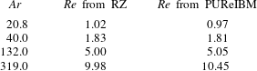
The sedimenting particle attains its terminal velocity when the hydrodynamic force acting on it balances its weight. For a given Archimedes number, the output of the simulation is a Reynolds number based on the terminal velocity and particle diameter. The terminal Reynolds number can be predicted using the Richardson–Zaki (RZ) correlation for the terminal velocity (Richardson & Zaki Reference Richardson and Zaki1954). The results presented in table 1 show that the terminal velocity obtained in PUReIBM simulations are in good agreement with that predicted by the RZ correlation. These results further establish the capability of PUReIBM to perform simulations of freely-evolving gas–solid suspensions. A summary of various applications of the PUReIBM PR-DNS strategy is given in Tenneti & Subramaniam (Reference Tenneti and Subramaniam2014). The simulation set-up that is used to perform PR-DNS of freely-evolving suspensions to quantify the steady-state source and dissipation of granular temperature, is discussed in the next section.
Comparison of the terminal Reynolds number obtained from PUReIBM simulations with that predicted by the RZ correlation for different Archimedes numbers.

5. Simulation set-up
The independent dimensionless parameters relevant to the study of freely-evolving gas–solid suspensions are the solid volume fraction
 ${\it\phi}$
, the solid-to-fluid density ratio
 ${\it\rho}_{p}/{\it\rho}_{f}$
and the Reynolds number based on the mean slip velocity
 $\mathit{Re}_{m}$
. The mean-slip Reynolds number is defined as
 $$\begin{eqnarray}\mathit{Re}_{m}=(1-{\it\phi})\frac{{\it\rho}_{f}\left|\left\langle \boldsymbol{W}\right\rangle \right|d_{p}}{{\it\mu}_{f}},\end{eqnarray}$$
where
 ${\it\mu}_{f}$
is the dynamic viscosity of the fluid phase. The mean slip velocity
 $\left\langle \boldsymbol{W}\right\rangle$
is defined as
 $\langle \boldsymbol{W}\rangle =\langle \boldsymbol{v}\rangle -\langle \boldsymbol{u}^{(f)}\rangle$
, and is the relative velocity between the solid-phase mean velocity and the fluid-phase mean velocity. Averaged quantities in these PR-DNS of statistically homogeneous flow are computed by first volume averaging the flow variable (e.g.
 $\langle \boldsymbol{u}^{(f)}\rangle$
) for one realization (corresponding to an initial particle configuration), and subsequently ensemble averaging over different particle configurations (corresponding to a specified average solid volume fraction, mean-slip Reynolds number and initial pair correlation function).
For a given triplet
 $\left({\it\phi},\mathit{Re}_{m},{\it\rho}_{p}/{\it\rho}_{f}\right)$
, the gas–solid suspension attains a steady granular temperature. The simulation set-up in the present study has been chosen to supply arbitrary values of
 $\left({\it\phi},\mathit{Re}_{m},{\it\rho}_{p}/{\it\rho}_{f}\right)$
as input, and keep them fixed during the course of the simulation. The task of maintaining a given
 $\mathit{Re}_{m}$
can be accomplished by specifying a mean pressure gradient that does not exactly balance the weight of the particles, but exerts the requisite body force to maintain the desired slip velocity between the particles and fluid. However, now both the mean particle velocity and the mean fluid velocity change in time because there is no steady solution in the laboratory frame to the mean momentum balance in each phase. Note that even though the mean phasic velocities are evolving in time, their difference – the mean slip velocity – attains a steady value.
The difficulty in simulating this flow set-up in the laboratory frame with periodic boundary conditions is that the continuous increase in fluid and particle velocities places unnecessary restrictions on the time step through the Courant condition. To circumvent this problem we use a different simulation set-up that performs the PR-DNS in an accelerating reference frame such that the particles have a zero mean velocity with respect to the computational grid. The advantage of this set-up is that the desired mean-slip Reynolds number is specified as an input parameter, and we are able to solve the problem with reasonable time steps that resolve the flow.
A homogeneous initial particle configuration is generated for the given solid volume fraction
 ${\it\phi}$
. The initial positions of the particles are obtained by equilibrating an ensemble of particles undergoing elastic collisions in the absence of interstitial fluid. The particles are advanced on a time step
 ${\rm\Delta}t_{\mathit{coll}}$
that is determined by the spring stiffness and the dashpot coefficients. The flow fields are updated on a time step
 ${\rm\Delta}t_{\mathit{fluid}}$
, which ensures that both the convective and viscous time scales are well resolved. At the start of a flow time step the forces acting on the particles are computed based on the flow fields obtained at the end of the previous flow time step. If
 ${\rm\Delta}t_{\mathit{coll}}$
is smaller than
 ${\rm\Delta}t_{\mathit{fluid}}$
the particles are stepped by
 ${\rm\Delta}t_{\mathit{coll}}$
until the end of the flow time step, otherwise both the particles and the fluid are stepped by
 ${\rm\Delta}t_{\mathit{coll}}$
. The simulation is continued until the granular temperature reaches a steady state.
The computational domain used is a cube with sides of length
 $L$
which is discretized using a regular Cartesian grid with
 $M$
grid cells in each direction so that
 ${\rm\Delta}x=L/M$
is the size of each grid cell. The spatial resolution is represented by the number of grid cells across the diameter of a particle, which is denoted
 $D_{m}=d_{p}/{\rm\Delta}x$
. For random arrangements of particles, the ratio
 $L/d_{p}$
is an independent parameter. The minimum box length is determined by the criterion that the spatial autocorrelation of flow statistics must decay to zero within the box. This is to prevent the periodicity of the numerical solution from leading to unphysical flow fields. The numerical parameter
 $L/d_{p}$
also determines the number of particles
 $N_{p}$
in the box such that for a given volume fraction
 ${\it\phi}_{}$
it is given by
 $$\begin{eqnarray}N_{p}=\left[\frac{6{\it\phi}}{{\rm\pi}}\left(\frac{L}{d_{p}}\right)^{3}\right],\end{eqnarray}$$
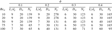
where the square brackets denote the nearest integer. The various numerical parameters used in the simulations are reported in table 2.
Numerical parameters (the ratio of the length of the box to the particle diameter
 $L/d$
, particle diameter in grid units
 $D_{m}$
, and number of particles
 $N_{p}$
) used in the simulations.
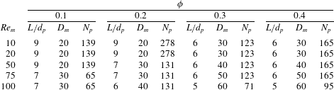
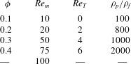
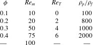
In the present study, PR-DNS of freely-evolving gas–solid suspensions are performed for solid volume fractions between 0.1 and 0.4 and for mean-slip Reynolds numbers between 10 and 100. The solid-to-fluid density ratio has been varied from 100 to 2000. Note that the lower limit of the density ratio corresponds to cork particles in air, while the upper limit is characteristic of glass beads suspended in air. The actual values of the physical parameters used in the simulations are provided in table 3. Simulations have been performed for each set of
 $\left({\it\phi},\mathit{Re}_{m},{\it\rho}_{p}/{\it\rho}_{f}\right)$
values, resulting in a total of 80 cases. For several cases, multiple independent simulations have been performed to ensure statistical convergence. Thus, more than 200 simulations are used to quantify the steady values of granular temperature, and the source and dissipation of granular temperature. These results are described in the subsequent sections.
Physical parameters (solid volume fraction, mean-slip Reynolds number, initial Reynolds number based on granular temperature and solid–fluid density ratio) used in PUReIBM simulations.
6. Quantification of steady-state source and dissipation of granular temperature
The simulation set-up described in the previous section has been used to perform PR-DNS of freely-evolving gas–solid suspensions initialized with different values of the granular temperature. When characterizing the effect of particle velocity fluctuations it is useful to define a Reynolds number based on the granular temperature
 $\mathit{Re}_{T}$
as:
 $$\begin{eqnarray}\mathit{Re}_{T}=\frac{{\it\rho}_{f}d_{p}\,T^{1/2}}{{\it\mu}_{f}}.\end{eqnarray}$$
Estimation of the granular temperature from PR-DNS is discussed in detail by Tenneti et al. (Reference Tenneti, Garg, Hrenya, Fox and Subramaniam2010). The temporal evolution of
 $T/\!\left|\left\langle \boldsymbol{W}\right\rangle \right|^{2}$
and
 $\mathit{Re}_{T}$
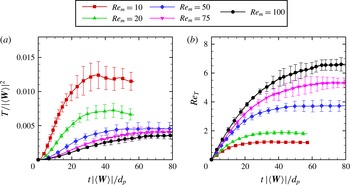
for a freely-evolving gas–solid suspension at a volume fraction of 0.1 and solid-to-fluid density ratio of 100, with different mean-slip Reynolds numbers is shown in figures 4(a) and 4(b), respectively. In these simulations all the particles start from rest and hence the initial
 $\mathit{Re}_{T}$
is zero. We observe that the granular temperature reaches a statistical steady state for all values of the mean-slip Reynolds number. In these simulations, a mean pressure gradient is applied to obtain the desired
 $\mathit{Re}_{m}$
, which results in a mean force
 $\left\langle \boldsymbol{F}\right\rangle$
acting on the suspension. The energy generated by the application of the mean pressure gradient,
 $\left\langle \boldsymbol{F}\right\rangle \boldsymbol{\cdot }\left\langle \boldsymbol{W}\right\rangle$
, is responsible for generation of velocity fluctuations in the fluid as well as in the particle phase. It has been shown by Mehrabadi et al. (Reference Mehrabadi, Tenneti, Garg and Subramaniam2015) that the fluid velocity fluctuations also attain a steady value.
(a) Temporal evolution of granular temperature normalized by the square of the magnitude of mean slip velocity for different mean-slip Reynolds number. The solid volume fraction is 0.1 and the solid to fluid density ratio of the suspension is 100. (b) Evolution of the Reynolds number based on granular temperature (
 $\mathit{Re}_{T}$
) for the cases shown in figure 4(a). Error bars are the 95 % confidence intervals obtained from five independent simulations.

From figure 4 we can also see that at a given solid-to-fluid density ratio and solid volume fraction, the normalized granular temperature decreases with increasing
 $\mathit{Re}_{m}$
(see figure 4
a, whereas
 $\mathit{Re}_{T}$
increases according to figure 4
b). This result implies that
 $T/\!\left|\left\langle \boldsymbol{W}\right\rangle \right|^{2}\sim 1/{\mathit{Re}_{m}}^{p}$
, such that
 $p<2$
. This result also implies that the granular temperature increases with mean slip velocity, and that is expected because particles pick up more energy from the fluid as
 $\mathit{Re}_{m}$
increases.
A pertinent question that needs to be answered is whether the steady granular temperature attained by the suspension for a given
 $\left({\it\phi},\mathit{Re}_{m},{\it\rho}_{p}/{\it\rho}_{f}\right)$
depends on the choice of the initial particle granular temperature. To answer this question, we selected a gas–solid suspension with
 ${\it\phi}=0.1$
,
 $\mathit{Re}_{m}=20,{\it\rho}_{p}/{\it\rho}_{f}=100$
, and initialized the particles with a Maxwellian velocity distribution corresponding to
 $\mathit{Re}_{T}=2$
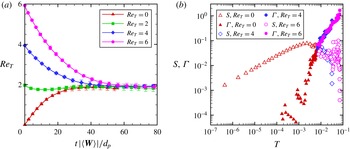
, 4, and 6. The temporal evolution of
 $\mathit{Re}_{T}$
is shown in figure 5(a). The evolution of
 $\mathit{Re}_{T}$
for a suspension initialized with a zero particle granular is also shown in the figure for reference. It is clear from the figure that the statistical steady state attained by the suspension is independent of the initial granular temperature. It is useful to examine the behaviour of source
 $S$
of (2.12) and dissipation
 ${\it\Gamma}$
of (2.13) with granular temperature for these suspensions to gain a better understanding of the flow physics. Figure 5(b) shows a phase-space plot
 $({\dot{T}},T)$
of (2.6) where the time derivative of temperature
 ${\dot{T}}$
is partitioned into source and dissipation terms. Figure 5(b) shows how all the gas–solid systems initialized with different granular temperatures arrive at the same stable steady state. The source and dissipation shown in this figure are computed from PR-DNS data using the estimators given in (B 1) and (B 2). In the suspension initialized with
 $\mathit{Re}_{T}=0$
, the particles pick up energy from the fluid and hence the source term (open triangles) is greater than dissipation (filled triangles) at initial time. Both source and dissipation grow from initially low values to their steady-state values. For the suspensions initialized with a granular temperature higher than the steady value, the particles have higher energy and thus they lose their energy to fluid. For these suspensions the dissipation (filled diamonds and filled circles) is initially greater than the source term (open diamonds and open circles).
(a) Temporal evolution of scaled granular temperature for suspensions initialized with different particle granular temperatures. The solid volume fraction is 0.1,
 $\mathit{Re}_{m}$
is 20 and
 ${\it\rho}_{p}/{\it\rho}_{f}$
is 100. The error bars represent the 95 % confidence intervals obtained from five independent realizations for each case. (b) Variation of source and dissipation with granular temperature for the suspensions shown in figure 5(a). The suspension initialized with
 $\mathit{Re}_{T}=2$
is not shown here. Filled symbols denote dissipation and open symbols denote the source.

Having established that the steady state attained by a gas–solid suspension is unique for a given
 $\left({\it\phi},\mathit{Re}_{m},{\it\rho}_{p}/{\it\rho}_{f}\right)$
, we now determine how the steady granular temperature
 $T_{SS}$
depends on these physical parameters. To the authors’ knowledge, this is the first report of the dependence of granular temperature on
 $\left({\it\phi},\mathit{Re}_{m},{\it\rho}_{p}/{\it\rho}_{f}\right)$
. Figure 6 shows the variation of
 $T_{SS}/\left|\left\langle \boldsymbol{W}\right\rangle \right|^{2}$
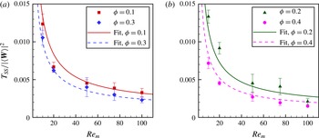
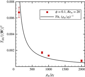
with solid volume fraction and mean-slip Reynolds number for a solid-to-fluid density ratio of 100. The steady scaled granular temperature decreases with both volume fraction and mean-flow Reynolds number. Figure 7 shows the behaviour of the steady scaled granular temperature with solid-to-fluid density ratio for a solid volume fraction of 0.2 and mean-flow Reynolds number of 20. As expected, the steady scaled granular temperature decreases with increasing inertia of the particles.
Variation of steady granular temperature with volume fraction and mean-flow Reynolds number for a density ratio of 100. Symbols are data obtained from PUReIBM PR-DNS and the solid lines indicate the fit given by (6.2). The error bars represent the 95 % confidence intervals obtained from five independent realizations for each case.

Variation of steady granular temperature with solid to fluid density ratio for a solid volume fraction of 0.1 and mean-flow Reynolds number 20. Symbols denote the data obtained from PUReIBM PR-DNS and the solid line indicates the function
 $\left({\it\rho}_{p}/{\it\rho}_{f}\right)^{-1}$
. The error bars represent the 95 % confidence intervals obtained from five independent realizations for each case.

It is interesting to note that the behaviour of the steady scaled granular temperature with
 $\mathit{Re}_{m}$
is similar to the behaviour of the scaled fluid kinetic energy with
 $\mathit{Re}_{m}$
reported by Mehrabadi et al. (Reference Mehrabadi, Tenneti, Garg and Subramaniam2015). Hence the functional dependence of the scaled
 $T_{SS}$
on
 $\mathit{Re}_{m}$
is similar to that proposed for the fluid kinetic energy (Mehrabadi et al.
Reference Mehrabadi, Tenneti, Garg and Subramaniam2015). As shown in figure 7,
 $\left({\it\rho}_{p}/{\it\rho}_{f}\right)^{-1}$
captures the dependence of
 $T_{SS}$
on the solid-to-fluid density ratio very well. Based on the data obtained from PUReIBM PR-DNS, the following functional form is proposed for the steady value of the scaled granular temperature:
 $$\begin{eqnarray}\displaystyle \frac{T_{SS}}{|\langle \boldsymbol{W}\rangle |^{2}} & = & \displaystyle \left\{[9.9(1-{\it\phi})^{1.23}\exp (-0.02(1-{\it\phi}){\mathit{Re}_{m}}^{0.28})]\left[1-\frac{1}{\exp ({\mathit{Re}_{m}}^{-0.8})}\right]\right.\nonumber\\ \displaystyle & & \displaystyle +\,\left.\frac{0.135(1-{\it\phi})}{\exp ({\mathit{Re}_{m}}^{-0.8})}\right\}({\it\rho}^{(p)}/{\it\rho}^{(f)})^{-1},\end{eqnarray}$$
which is valid in the range
 $0.1\leqslant {\it\phi}\leqslant 0.4$
,
 $10\leqslant \mathit{Re}_{m}\leqslant 100$
and
 $100\leqslant {\it\rho}_{p}/{\it\rho}_{f}\leqslant 2000$
.
6.1. Physical significance of the acceleration–velocity covariance as source and sink of granular temperature
Scatter plots in the
 $\boldsymbol{v}^{\prime \prime }{-}\boldsymbol{A}_{h}^{\prime \prime }$
phase space can be reconciled with the source and dissipation of granular temperature during the evolution of
 $T$
(Subramaniam et al.
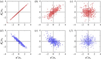
Reference Subramaniam, Mehrabadi, Horwitz and Mani2014). Figure 8 shows the fluctuating velocity–acceleration scatter plot from PR-DNS for the case with
 ${\it\phi}=0.1$
and
 $Re_{m}=20$
at initial time and at steady state for two different cases corresponding to particles initialized with
 $Re_{T}=0$
and
 $6$
. The points that lie in quadrants 1 and 3 contribute to the hydrodynamic source
 $S_{h}$
of
 $T$
whereas those in quadrants 2 and 4 contribute to the hydrodynamic dissipation
 ${\it\Gamma}_{h}$
(cf. (2.6)).
Scatter plot of
 $\boldsymbol{v}^{\prime \prime }{-}\boldsymbol{A}_{h}^{\prime \prime }$
that corresponds to the quantification of the hydrodynamic source and dissipation of granular temperature for the case with
 ${\it\phi}=0.1$
and
 $Re_{m}=20$
. (a–c) Corresponds to the case initialized with
 $Re_{T}=0$
, while (d–f) belongs to the case initialized with
 $Re_{T}=6$
. The data in (a,d), (b,e) and (c,f) are, respectively, extracted at early time, intermediate time and at steady state. In these plots, the horizontal axes are normalized by the standard deviation of particle velocity fluctuations, and the vertical axes are normalized by the standard deviation of fluctuating hydrodynamic accelerations.

Figure 8(a) shows that when the particles evolve from initially being at at rest, at early time all points in the
 $\boldsymbol{v}^{\prime \prime }{-}\boldsymbol{A}_{h}^{\prime \prime }$
phase space contribute solely to the hydrodynamic source of
 $T$
. As time progresses the particles gain energy. Therefore, some of the scatter points now contribute to the dissipation, although their major contribution is still to the source of
 $T$
, as demonstrated in figure 8(b). Once the suspension reaches steady state, the points in the
 $\boldsymbol{v}^{\prime \prime }{-}\boldsymbol{A}_{h}^{\prime \prime }$
plane are finally uniformly distributed, contributing equally to source and dissipation as shown in figure 8(c). On the other hand, when the particles are initialized with a velocity variance that is higher than the steady value of
 $T$
for those
 ${\it\phi}$
and
 $Re_{m}$
, the majority of points in the
 $\boldsymbol{v}^{\prime \prime }{-}\boldsymbol{A}_{h}^{\prime \prime }$
phase-space scatter plot contribute to the dissipation of
 $T$
, as seen in figure 8(d). As the simulation progresses, some of the points migrate to the source quadrants of the scatter plot as shown in figure 8(e). Finally, all the points are uniformly distributed in the
 $\boldsymbol{v}^{\prime \prime }{-}\boldsymbol{A}_{h}^{\prime \prime }$
phase space at steady state, as demonstrated in figure 8(f). These results give a clear physical picture of the role of source and dissipation arising from hydrodynamic contributions to the particle acceleration in determining the evolution of particle granular temperature.
At steady state, the source and dissipation are equal and hence (2.11) reads,
 ${\it\Gamma}_{SS}=S_{SS}$
. Here the subscript
 $SS$
denotes the values of source and dissipation at steady state. In order to non-dimensionalize the source, we need to define acceleration and velocity scales. For the acceleration scale, we use the acceleration generated due to the Stokes drag acting on a particle moving with a velocity of
 $(1-{\it\phi})\left\langle \boldsymbol{W}\right\rangle$
. Note that
 $(1-{\it\phi})\left\langle \boldsymbol{W}\right\rangle$
is the superficial velocity that is commonly used to non-dimensionalize the drag force in widely used drag correlations. Hence we use the superficial velocity here as a velocity scale. The steady source
 $S_{SS}$
is reported in the following non-dimensional form:
 $$\begin{eqnarray}S_{SS}^{\ast }=\frac{mS_{SS}}{3{\rm\pi}{\it\mu}_{f}d_{p}\left(1-{\it\phi}\right)^{2}\left|\left\langle \boldsymbol{W}\right\rangle \right|^{2}},\end{eqnarray}$$
where
 $m$
is the mass of the particle and
 ${\it\mu}_{f}$
is the dynamic viscosity of the fluid.
Behaviour of the non-dimensional steady source
 $S_{SS}^{\ast }$
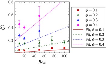
with volume fraction and Reynolds number for a solid-to-fluid density ratio of 100. Symbols indicate PUReIBM DNS data and solid lines indicate the fit given by (6.5). The error bars represent the 95 % confidence intervals obtained from five independent realizations for each case.

Figure 9 shows the behaviour of the normalized steady source with volume fraction and mean-flow Reynolds number for a solid to fluid density ratio of 100. The normalized source increases with both volume fraction and Reynolds number. This behaviour can be explained by employing a simple scaling analysis. Since the source of granular temperature is caused by the correlation of particle acceleration fluctuations and particle velocity fluctuations, the source scales as
 $S_{SS}\sim {\it\sigma}_{A}T_{SS}^{1/2}$
, where
 ${\it\sigma}_{A}$
is the standard deviation in the particle acceleration. This scaling implies that the normalized source scales as
 $$\begin{eqnarray}S_{SS}^{\ast }=\frac{mS_{SS}}{3{\rm\pi}{\it\mu}_{f}d_{p}\left(1-{\it\phi}\right)^{2}\left|\left\langle \boldsymbol{W}\right\rangle \right|^{2}}\sim \frac{{\it\sigma}_{A}}{\left|\left\langle \boldsymbol{A}\right\rangle \right|}\frac{F\left({\it\phi},\mathit{Re}_{m}\right)}{\left(1-{\it\phi}\right)}\left(\frac{T_{SS}}{\left|\left\langle \boldsymbol{W}\right\rangle \right|^{2}}\right)^{1/2},\end{eqnarray}$$
where
 $F\left({\it\phi}_{},\mathit{Re}_{m}\right)$
is the normalized mean drag per particle which increases with both solid volume fraction and mean-flow Reynolds number. Although the steady scaled granular temperature decreases with both solid volume fraction and Reynolds number, the strong dependence of the mean drag on
 ${\it\phi}$
determines the overall behaviour of the normalized source term. The dependence of the normalized source on the solid-to-fluid density ratio is determined by the dependence of steady granular temperature on
 ${\it\rho}_{p}/{\it\rho}_{f}$
. Indeed, PUReIBM DNS data indicate that
 $S_{SS}^{\ast }$
varies inversely with
 $({\it\rho}_{p}/{\it\rho}_{f})^{1/2}$
. Equation (6.4) implies that the dependence of
 $S_{SS}^{\ast }$
on
 ${\it\phi}$
and
 $\mathit{Re}_{m}$
should be similar to the dependence of the normalized drag on
 ${\it\phi}$
and
 $\mathit{Re}_{m}$
. Using the drag law proposed by Tenneti et al. (Reference Tenneti, Garg and Subramaniam2011), the following functional form is proposed as a fit to the PR-DNS data for the normalized steady source:
 $$\begin{eqnarray}S_{SS}^{\ast }\left({\it\phi},\mathit{Re}_{m},\frac{{\it\rho}_{p}}{{\it\rho}_{f}}\right)=\left(1+0.035\mathit{Re}_{m}\right)\frac{{\it\phi}}{\left(1-{\it\phi}\right)^{3}}\left(\frac{{\it\rho}_{p}}{{\it\rho}_{f}}\right)^{-1/2},\end{eqnarray}$$
which is valid in the range
 $0.1\leqslant {\it\phi}\leqslant 0.4$
,
 $10\leqslant \mathit{Re}_{m}\leqslant 100$
and
 $100\leqslant {\it\rho}_{p}/{\it\rho}_{f}\leqslant 2000$
. Clearly a better fit to the data shown in figure 9 is possible, but it might be harder to ascribe a physical interpretation to that functional form. Therefore, we have not attempted that here but further research in this direction could be pursued. The functional forms for steady temperature and source given by (6.2) and (6.5) are now used to develop a Lagrangian model for particle acceleration due to hydrodynamic forces that is described in the next section.
7. Lagrangian model for hydrodynamic acceleration of particles
As discussed earlier, the closure model for the conditional particle acceleration affects both the mean momentum and the particle granular temperature, as these are derived from the NDF equation (2.1). A closure at the one-particle distribution level automatically implies closure of the mean momentum and particle velocity second-moment equations. Furthermore, closures at the one-particle distribution level are guaranteed to satisfy realizability criteria, whereas special care is needed to ensure the same in the case of moment closures. These considerations motivate the development of models for the unclosed terms in the transport equation for the one-particle distribution function corresponding to gas–solid flow.
The model for the instantaneous particle acceleration can be deduced by considering the factors that contribute to the hydrodynamic forces acting on a particle. In a typical gas–solid flow system, the presence of numerous particles moving in different directions will lead to continuously changing hydrodynamic interactions between particles (i.e. fluctuations in the fluid velocity and pressure fields). We propose the following stochastic model for the increment in the particle velocity:
 $$\begin{eqnarray}\text{d}v_{i}^{}=-{\it\beta}\langle W_{i}\rangle \,\text{d}t-{\it\gamma}v_{i}^{\prime \prime }\,\text{d}t+B\,\text{d}\mathscr{W}_{i}.\end{eqnarray}$$
The above equation is an isotropic form of the generalized Langevin model (Haworth & Pope Reference Haworth and Pope1986). In the above equation
 $\text{d}v_{i}^{}$
is the increment in the particle velocity,
 $v_{i}^{\prime \prime }$
is the fluctuation in the particle velocity and
 $\text{d}\mathscr{W}_{i}$
is a Wiener process increment. Fluctuations in the particle velocity are defined about the mean particle velocity, i.e.
 $v_{j}^{^{\prime \prime }}=v_{j}-\langle v_{j}\rangle$
. The model coefficients
 ${\it\beta}$
,
 ${\it\gamma}$
and
 $B$
will be specified in § 7.2. The first term on the right-hand side of (7.1) represents the mean acceleration experienced by the solid phase in the suspension, and accounts for the effect of the mean slip velocity. This term is related to the normalized force
 $F$
as defined by Hill et al. (Reference Hill, Koch and Ladd2001b
) and Tenneti et al. (Reference Tenneti, Garg and Subramaniam2011) as follows:
 $$\begin{eqnarray}F=\frac{m{\it\beta}\left|\left\langle \boldsymbol{W}\right\rangle \right|}{3{\rm\pi}{\it\mu}_{f}D\left(1-{\it\phi}\right)\left|\left\langle \boldsymbol{W}\right\rangle \right|}.\end{eqnarray}$$
The coefficient
 ${\it\beta}$
can thus be inferred by computing
 $F$
using any of the drag laws developed for gas–solid suspensions (Hill et al.
Reference Hill, Koch and Ladd2001a
,Reference Hill, Koch and Ladd
b
; van der Hoef et al.
Reference van der Hoef, Beetstra and Kuipers2005; Beetstra et al.
Reference Beetstra, van der Hoef and Kuipers2007; Yin & Sundaresan Reference Yin and Sundaresan2009a
,Reference Yin and Sundaresan
b
; Holloway et al.
Reference Holloway, Yin and Sundaresan2010; Tenneti et al.
Reference Tenneti, Garg and Subramaniam2011). The second term accounts for the fluctuation in the particle velocity and the last term models the effect of the hydrodynamic interaction of the neighbouring particles. The coefficient
 ${\it\gamma}$
is the inverse of the Lagrangian particle velocity autocorrelation time. It quantifies how long a particle retains memory of its initial velocity. These coefficients are functions of volume fraction
 ${\it\phi}$
, mean-flow Reynolds number
 $\mathit{Re}_{m}$
and particle-to-fluid density ratio
 ${\it\rho}_{p}/{\it\rho}_{f}$
. It is interesting to note that in the different problems of dilute, turbulent particle-laden Couette (Goswami & Kumaran Reference Goswami and Kumaran2010a
,Reference Goswami and Kumaran
b
) and channel flows (Goswami & Kumaran Reference Goswami and Kumaran2011, Reference Goswami and Kumaran2010c
), Goswami & Kumaran found that the effect of fluid velocity fluctuations on particle acceleration can be described using a Langevin equation. The Langevin model for the particle acceleration we propose here is verified by computing the particle velocity autocorrelation function after the granular temperature reaches a steady state. Following a standard approach in PDF modelling of turbulent reacting flows (Pope Reference Pope1985, Reference Pope2000), this stochastic model based on the Langevin equation is developed for a statistically stationary problem with model coefficients that depend on moments of the PDF (e.g. mean velocity or second moments). The model is intended to be then applied to the non-stationary problem with local values of the temporally varying mean and second moments that appear in the model coefficients. This approach makes the assumption of local statistical stationarity.
7.1. Verification of the Langevin model for inertial particle acceleration
To verify the particle acceleration model, we consider the increment in the particle’s Lagrangian velocity fluctuation:
 $$\begin{eqnarray}\text{d}v_{i}^{\prime \prime }=v_{i}^{\prime \prime }(t+\text{d}t)-v_{t}^{\prime \prime }(t)=-{\it\gamma}v_{i}^{\prime \prime }\,\text{d}t+B\,\text{d}\mathscr{W}_{i}.\end{eqnarray}$$
As described earlier, the model coefficient
 ${\it\gamma}$
in the above equation is the inverse of the integral time scale of the particle’s velocity autocorrelation. The particle velocity autocorrelation function
 ${\it\rho}(s)$
is defined as follows:
 $$\begin{eqnarray}{\it\rho}(s)=\frac{\langle v_{i}^{\prime \prime }(t_{0})v_{i}^{\prime \prime }(t_{0}+s)\rangle }{\langle v_{k}^{\prime \prime }(t_{0})v_{k}^{\prime \prime }(t_{0})\rangle },\end{eqnarray}$$
where
 $s$
is the separation in time. The integral time scale for the autocorrelation function is defined as
 $T_{L}=\int _{0}^{\infty }{\it\rho}(s)\,\text{d}s$
. Using this definition, we computed the integral time scale from PR-DNS after the granular temperature reached a steady state. If a stochastic process obeys the Langevin equation with an integral time scale of
 $T_{L}$
, then its autocorrelation function should decay exponentially, i.e.
 ${\it\rho}(s)=\text{e}^{-s/T_{L}}$
. We extracted the autocorrelation function from PR-DNS and compared it with the exponential function predicted by the Langevin model. This comparison is shown in figure 10. Therefore, we conclude that for both density ratios considered, the evolution of the autocorrelation function obtained from PR-DNS matches with the exponential decay predicted by the Langevin model. It should be noted that the behaviour of PR-DNS data for the particle velocity autocorrelation will not match the exponential decay implied by the Langevin model at small separation times
 $s$
because the PR-DNS data is continuous and differentiable whereas the Langevin model is continuous but non-differentiable (Pope Reference Pope2000). This discrepancy at small separation times
 $s$
could be overcome by using a second-order Langevin model for the particle acceleration (Sawford Reference Sawford1991), and could be the subject of future studies. At any given volume fraction, mean-flow Reynolds number and solid-to-fluid density ratio, we need to specify the coefficients as a function of the granular temperature so that we can predict the evolution of the suspension using the Langevin model. The procedure to specify the model coefficients from PR-DNS is presented next.
Verification of the Langevin model. (a) Compares the particle velocity autocorrelation function extracted from PR-DNS of freely-evolving suspension (volume fraction of 0.2, mean-flow Reynolds number of 20 and solid-to-fluid density ratio of 10) with the exponential decay predicted by the Langevin model. (b) Is the same as (a) for a suspension with solid-to-fluid density of 100. Reproduced from Garzó et al. (Reference Garzó, Tenneti, Subramaniam and Hrenya2012) with permission.

7.2. Specification of the model coefficients
The objective of the particle acceleration model is to predict the evolution of the granular temperature correctly. In order to achieve this we have to match the source
 $S$
and dissipation
 ${\it\Gamma}$
in (2.11) with those predicted by the model given by (7.1). The evolution of the granular temperature
 $T^{\ast }$
predicted by the Langevin model is given by:
 $$\begin{eqnarray}\frac{\text{d}T^{\ast }}{\text{d}t}=-2{\it\gamma}T^{\ast }+B^{2}.\end{eqnarray}$$
Comparing (2.11) and (7.5), the model coefficients
 ${\it\gamma}$
and
 $B$
can be written as follows:
 $$\begin{eqnarray}\displaystyle & \displaystyle {\it\gamma}=\frac{{\it\Gamma}\left({\it\phi},\mathit{Re}_{m},{\it\rho}_{p}/{\it\rho}_{f}\right)}{2T}, & \displaystyle\end{eqnarray}$$
 $$\begin{eqnarray}\displaystyle & B^{2}=S\left({\it\phi},\mathit{Re}_{m},{\it\rho}_{p}/{\it\rho}_{f}\right). & \displaystyle\end{eqnarray}$$
 ${\it\gamma}$
and
 $B^{2}$
are also time-dependent functions of many parameters. It is desirable to find a scaling for the source (and dissipation) to deduce simple forms that characterize their dependence on these parameters. This motivates us to seek a self-similar description of the granular temperature evolution equation that enables us to obtain expressions for the time-dependent source and dissipation terms as self-similar departures from their steady values that are parametrized by
 ${\it\phi}$
,
 $\mathit{Re}_{m}$
and
 ${\it\rho}_{p}/{\it\rho}_{f}$
. We introduce the following scaling for the excess temperature
 ${\it\theta}$
, source and dissipation respectively:
 $$\begin{eqnarray}\displaystyle & \displaystyle {\it\theta}=\frac{T-T_{SS}}{T_{SS}}, & \displaystyle\end{eqnarray}$$
 $$\begin{eqnarray}\displaystyle & \displaystyle {\hat{S}}=\frac{S-S_{SS}}{S_{SS}}, & \displaystyle\end{eqnarray}$$
 $$\begin{eqnarray}\displaystyle & \displaystyle \hat{{\it\Gamma}}=\frac{{\it\Gamma}-{\it\Gamma}_{SS}}{{\it\Gamma}_{SS}}, & \displaystyle\end{eqnarray}$$
 ${\hat{S}}({\it\theta})$
and
 $\hat{{\it\Gamma}}({\it\theta})$
are solely dependent on the excess temperature
 ${\it\theta}$
. The model coefficients can now be cast in the following form:
 $$\begin{eqnarray}\displaystyle & \displaystyle {\it\gamma}=\frac{1}{2}\left(\frac{\hat{{\it\Gamma}}\left({\it\theta}\right)+1}{{\it\theta}+1}\right)\frac{S_{SS}\left({\it\phi},\mathit{Re}_{m},{\it\rho}_{p}/{\it\rho}_{f}\right)}{T_{SS}\left({\it\phi},\mathit{Re}_{m},{\it\rho}_{p}/{\it\rho}_{f}\right)}, & \displaystyle\end{eqnarray}$$
 $$\begin{eqnarray}\displaystyle & \displaystyle B^{2}=({\hat{S}}({\it\theta})+1)S_{SS}\left({\it\phi},\mathit{Re}_{m},{\it\rho}_{p}/{\it\rho}_{f}\right). & \displaystyle\end{eqnarray}$$
 ${\hat{S}}$
and
 $\hat{{\it\Gamma}}$
on the excess temperature. We propose the following functional forms to model the non-dimensional source and dissipation:
 $$\begin{eqnarray}\displaystyle & {\hat{S}}=\left\{\begin{array}{@{}ll@{}}1-\text{e}^{(A{\it\theta}+B{\it\theta}^{2}+C{\it\theta}^{3}+D{\it\theta}^{4})},\quad & {\it\theta}\leqslant 0,\\ E+\displaystyle \frac{1+F}{1+\text{e}^{(G+H{\it\theta})}},\quad & {\it\theta}>0,\end{array}\right. & \displaystyle\end{eqnarray}$$
 $$\begin{eqnarray}\displaystyle & \displaystyle \hat{{\it\Gamma}}=\left\{\begin{array}{@{}ll@{}}\displaystyle \frac{\text{e}^{{\it\theta}+1}-{\it\theta}-e}{e-2},\quad & {\it\theta}\leqslant 0,\\ 2{\it\theta},\quad & {\it\theta}>0,\end{array}\right. & \displaystyle\end{eqnarray}$$
 $A=9.296$
,
 $B=26.182$
,
 $C=33.863$
,
 $D=17.67$
,
 $E=-0.634$
,
 $F=0.599$
,
 $G=0.420$
and
 $H=2.969$
.
Scaling of source and dissipation with granular temperature in non-dimensional phase space (volume fraction of 0.1, mean-flow Reynolds number of 20 and solid-to-fluid density ratio of 100) with particles being initialized with
 $Re_{T}=0$
(▵), 4 (♢), and 6 (○). Hollow symbols denote the source, while filled symbols denote dissipation. The error bars represent the 95 % confidence intervals obtained from five independent realizations for each case. The solid lines are the curve fits for source and dissipation given by (7.13) and (7.14), respectively.

In order to complete the specification of the model coefficients we use the functional forms for the dependence of steady granular temperature and source on the solid volume fraction, mean-flow Reynolds number and the solid-to-fluid density ratio, which have been proposed in § 6.
8. Model assessment
In order to assess the performance of the proposed model, we implemented the particle acceleration model presented in the previous section in MFIX-DEM. In this code, the change in the velocity of the particles due to the hydrodynamic forces is given by (7.1). The change in velocity due to inter-particle collisions is modelled using the same soft-sphere collision model that was described in the PR-DNS numerical method. For a direct assessment of the performance of the model, the simulations are performed in the same periodic cubic domains that were used in the PR-DNS. Moreover, only a single cell is used so as to remove the effects of spatial discretization on the model assessment. Details about the numerical convergence of the implemented model with respect to time step and the number of particles are given in appendix C.
The first objective is to assess the impact of the particle acceleration model on the evolution of granular temperature. For this purpose, we selected a gas–solid suspension with
 $\mathit{Re}_{m}=10$
,
 ${\it\phi}=0.1$
, and
 ${\it\rho}_{p}/{\it\rho}_{f}=100$
, and initialized the particles with different initial granular temperatures. We performed these simulations with both the Lagrangian model for particle acceleration due to hydrodynamic forces that is based on simple extension of the mean drag law (see appendix A for details) and with the Langevin model proposed in this work. The evolution of granular temperature is shown in figure 12 (the results with the Lagrangian model based on simple extension of the mean drag law are denoted ‘without LM’ in the legend). We see that for different initial granular temperatures, the steady-state granular temperature obtained is the same. Moreover, the figure shows that, as expected from the analysis in appendix A, the granular temperature for the Lagrangian model based on simple extension of the mean drag law decays to zero as there is no source term in the evolution equation of the granular temperature. Only by using the stochastic Lagrangian model for hydrodynamic acceleration is a finite steady granular temperature obtained. Also, as a verification, the moment equation (2.11) was solved using Matlab and the comparison shows that the MFIX-DEM results are in accordance with the moment equation.
Evolution of granular temperature with different initial granular temperatures.

Next we study how well the steady state proposed in § 6 is attained by gas–solid suspensions that are simulated using the acceleration model. For this we performed MFIX-DEM simulations at different solid volume fractions and mean-slip Reynolds numbers at a density ratio of 100. Figure 13 shows that the model predicts the steady-state granular temperature values very close to the fit proposed in (6.2). The maximum error in MFIX-DEM simulation results is around 5 % from the correlation value which is reasonable. As the correlation is obtained from the PUReIBM data corresponding to a wide range of volume fractions and mean-slip Reynolds numbers, the model could be applied to various regions in a riser flow in continuum simulations to compute the local granular temperature based on the local (cell) mean-slip Reynolds number and local volume fraction. This in turn would lead to a better prediction of particle velocities which is essential for understanding the mean flow structure in riser flows.
Comparison of steady-state granular temperatures for various
 ${\it\phi}$
and
 $Re_{m}$
obtained from MFIX-DEM with the correlation proposed in (6.2).

9. Discussion
As noted earlier, the objective of this paper is to develop a Lagrangian particle acceleration model that reproduces the granular temperature evolution correctly. Such a Lagrangian particle acceleration model can be used in LE simulations of gas–solid flows. Although the advantage of the Langevin model is a closure of the conditional acceleration term in the NDF transport equation, assuming a Langevin form for the particle acceleration introduces certain closure assumptions, such as exponential decay of the Lagrangian velocity autocorrelation. Therefore, although the Langevin model is guaranteed to reproduce the steady granular temperature by construction, it will likely introduce modelling errors into higher-order statistics. It is useful to consider the regime of validity of the model developed in this paper that is based on PR-DNS. In the PR-DNS the particles are initially at rest and they eventually attain a steady granular temperature that is independent of the initial condition. We verified that even initializing the particles with a granular temperature higher than the steady value results in relaxation back to the steady value (see figure 5 a). The relatively low levels of steady granular temperature that are observed in the PR-DNS indicate that the flow is not dominated by collisions (Mehrabadi et al. Reference Mehrabadi, Tenneti, Garg and Subramaniam2015). Therefore, the model developed in this work is applicable in such situations. Visual observation of particles in fluidized bed risers (Cocco et al. Reference Cocco, Shaffer, Hays, Reddy Karri and Knowlton2010) indicate that such levels of granular temperature are indeed found even in inhomogeneous flows. However, in certain gas–solid flow applications it is possible that the presence of mean shear or the injection of particles with high velocity fluctuations could result in higher particle (and fluid) velocity fluctuations, and those might merit separate consideration.
The importance of the source of granular temperature arising from hydrodynamic interactions has important implications for the stability of gas–solid flow. Instabilities in gas–solid flow are closely linked to the appearance of local regions of low granular temperature associated with particle clustering, and the accurate representation of granular temperature evolution through the particle acceleration model is important. Specifically, most CFD-DEM or LES-DEM models currently use deterministic particle acceleration models that are based on a simple extension of average drag models applied with local estimates of the solid volume fraction and Reynolds number. The granular temperature equation implied by such models may not accurately capture the PR-DNS predictions described in this work. Finally, it should be noted that the PR-DNS results are themselves dependent on the choice of ensemble. In this work and in all other published homogeneous PR-DNS studies, the ensemble corresponds to holding the quantities
 $(N,{\it\phi},\mathit{Re}_{m})$
, viz. total number of particles, mean solid volume fraction and mean-slip Reynolds number, constant. The extent to which such an ensemble corresponds to experimental observations of locally homogeneous gas–solid flow ultimately determines the applicability of these findings.
10. Conclusions
Particle acceleration in statistically homogeneous gas–solid suspensions affects the evolution of the particle granular temperature. Accurate prediction of the evolution of the particle granular temperature in device-scale CFD simulations is important for capturing the physical phenomena of interest in such simulations. A Langevin equation is proposed to model the Lagrangian particle acceleration due to hydrodynamic forces in gas–solid suspensions at moderate Reynolds numbers. This acceleration model includes the effect of the presence of neighbour particles and particle velocity fluctuations, in addition to the steady drag force. The coefficients of the model are obtained at moderate Reynolds numbers by performing PR-DNS of freely-evolving gas–solid suspensions using the PUReIBM methodology.
A key finding that emerges from this work is that at steady state the Lagrangian particle velocity autocorrelation function decays exponentially, thus justifying the use of a Langevin-like model to describe the increment in particle velocity. The coefficients of the particle acceleration model are related to the source and dissipation of granular temperature using the fluctuation–dissipation theorem. Expressions to uniquely compute the source and sink of granular temperature from PR-DNS are derived.
PUReIBM simulations of freely-evolving suspensions are performed over a wide range of relevant fluid and particle properties We considered four values of volume fraction (
 ${\it\phi}_{}=0.1$
, 0.2, 0.3 and 0.4), five values of mean-flow Reynolds number (
 $\mathit{Re}_{m}=10$
, 20, 50, 75 and 100) and four values of solid-to-fluid density ratio (
 ${\it\rho}_{p}/{\it\rho}_{f}=100$
, 800, 1000 and 2000). These physical parameters result in gas–solid suspensions with a low steady particle granular temperature that are not dominated by particle collisions, which is characteristic of fluidized bed risers. By defining similarity variables as departures from the steady-state values, we reduce the model specification to determine the functional dependence of only three functions. We determined the functional dependence of the non-dimensional source and dissipation on the non-dimensional granular temperature. We developed the functional dependence of steady-state source and granular temperature on solid volume fraction, mean-slip Reynolds number and solid-to-fluid density ratio.
The stochastic acceleration model can be used in CFD-DEM simulations of gas–solid flow as well as in direct quadrature method of moments. The expressions for source and dissipation of granular temperature at moderate Reynolds numbers determined in this work can also be used in Eulerian two-fluid simulations and also in deriving kinetic theory closures for gas–solid flow (Garzó et al. Reference Garzó, Tenneti, Subramaniam and Hrenya2012).
Acknowledgements
This work was partially supported by a Department of Energy grant DE-FC26-07NT43098 through the National Energy Technology Laboratory and by a National Science Foundation grant CBET 1134500. The authors would like to thank R. Fox for useful suggestions related to the stochastic model for particle acceleration, K. Devendran for performing the MFIX-DEM simulations, and W. Fullmer for a careful reading of an early draft of the manuscript.
Appendix A. Lagrangian model for hydrodynamic acceleration of a particle from simple extension of average drag law
The trajectory of a solid particle in a gas–solid flow can be represented in Lagrangian coordinates
 $\{\boldsymbol{x}(t),\boldsymbol{v}(t)\}$
that evolve according to Newtonian dynamics as
 $$\begin{eqnarray}\displaystyle & \displaystyle \frac{\text{d}\boldsymbol{x}}{\text{d}t}=\boldsymbol{v}, & \displaystyle\end{eqnarray}$$
 $$\begin{eqnarray}\displaystyle & \displaystyle \frac{\text{d}\boldsymbol{v}}{\text{d}t}=\boldsymbol{A}_{h}+\boldsymbol{A}_{c}, & \displaystyle\end{eqnarray}$$
 $\boldsymbol{A}_{h}$
and
 $\boldsymbol{A}_{c}$
represent the acceleration due to hydrodynamic and collisional forces, respectively. The instantaneous acceleration due to hydrodynamic forces is often modelled by simple extension of the average drag on the particles in the suspension
 $\langle \boldsymbol{A}_{h}\rangle =-{\it\beta}(\langle \boldsymbol{v}\rangle -\langle \boldsymbol{u}^{(f)}\rangle )$
, where the angle brackets represent ensemble averages, and
 ${\it\beta}$
is the inverse momentum response time corresponding to the drag model that can depend on the mean-slip Reynolds number and solid volume fraction. Replacing the average particle velocity
 $\langle \boldsymbol{v}\rangle$
with the instantaneous particle velocity
 $\boldsymbol{v}$
yields the simple model for the instantaneous acceleration:
 $$\begin{eqnarray}\boldsymbol{A}_{h}={\it\beta}(\langle \boldsymbol{u}^{(f)}\rangle -\boldsymbol{v}).\end{eqnarray}$$
We now derive the particle velocity variance corresponding to this acceleration model for statistically homogeneous gas–solid flow. Substituting the model for hydrodynamic acceleration into (A 2) and averaging over the ensemble of particles results in the evolution of mean particle velocity as
 $$\begin{eqnarray}\frac{\text{d}\langle \boldsymbol{v}\rangle }{\text{d}t}=-{\it\beta}(\langle \boldsymbol{v}\rangle -\langle \boldsymbol{u}^{(f)}\rangle ).\end{eqnarray}$$
Note that in the above expression, the mean collisional acceleration is zero, i.e.
 $\langle \boldsymbol{v}\rangle$
due to the conservation of linear momentum between a pair of colliding particles. To derive an equation for the fluctuating velocity of the particle defined as
 $\boldsymbol{v}^{\prime \prime }=\boldsymbol{v}-\langle \boldsymbol{v}\rangle$
, one should subtract the above equation from the instantaneous velocity equation given by (A 2), which leads to the following expression:
 $$\begin{eqnarray}\frac{\text{d}\boldsymbol{v}^{\prime \prime }}{\text{d}t}=-{\it\beta}\boldsymbol{v}^{\prime \prime }+\boldsymbol{A}_{c}.\end{eqnarray}$$
The evolution equation of the granular temperature (trace of the particle velocity covariance) can be obtained by computing the dot product of the above expression by
 $\boldsymbol{v}^{\prime \prime }$
, and then averaging over the ensemble of particles, which results in:
 $$\begin{eqnarray}\frac{\text{d}T}{\text{d}t}=-\frac{2}{3}{\it\beta}\langle \boldsymbol{v}^{\prime \prime }\boldsymbol{\cdot }\boldsymbol{v}^{\prime \prime }\rangle +\frac{2}{3}\langle \boldsymbol{v}^{\prime \prime }\boldsymbol{\cdot }\boldsymbol{A}_{c}\rangle .\end{eqnarray}$$
The first term on the right-hand side of the above equation contains the hydrodynamic source and dissipation as described in § 2. Similarly, the second term on the right-hand side includes the collisional source and dissipation. Note that since particle collisions do not generate energy, they cannot contribute to the source of
 $T$
. For inelastic collisions where there is energy loss during collision, the collisional dissipation can be non-zero. However, for elastic collisions the conservation of energy necessitates that the collisional dissipation of
 $T$
be zero. In either case, this simple model for the hydrodynamic particle acceleration dictates that the granular temperature decays to zero from its initial value at all mean-slip Reynolds numbers, irrespective of the collision model.
Appendix B. Estimation of source and dissipation of granular temperature from PR-DNS
Equations (2.12) and (2.13) give the analytical expressions for source and dissipation of particle granular temperature. The following estimators can be used to compute the source and dissipation from PR-DNS of a statistically homogeneous gas–solid suspension:
 $$\begin{eqnarray}\displaystyle & \displaystyle S_{E}=-\frac{2}{3}\frac{1}{N_{p}}\mathop{\sum }_{n=1}^{N_{p}}{\it\zeta}_{-}^{(n)}{v_{i}^{\prime \prime }}^{(n)}{v_{i}^{\prime \prime }}^{(n)}, & \displaystyle\end{eqnarray}$$
 $$\begin{eqnarray}\displaystyle & \displaystyle {\it\Gamma}_{E}=\frac{2}{3}\frac{1}{N_{p}}\mathop{\sum }_{n=1}^{N_{p}}{\it\zeta}_{+}^{(n)}{v_{i}^{\prime \prime }}^{(n)}{v_{i}^{\prime \prime }}^{(n)}. & \displaystyle\end{eqnarray}$$
 $n$
th particle is denoted
 $A^{\prime \prime (n)}$
and the fluctuation in the velocity is denoted
 $v^{\prime \prime (n)}$
. In the above expressions for source and dissipation,
 ${\it\zeta}_{+}^{(n)}=({\it\zeta}_{}^{(n)}+|{\it\zeta}_{}^{(n)}|)/2$
and
 ${\it\zeta}_{-}^{(n)}=({\it\zeta}_{}^{(n)}-|{\it\zeta}_{}^{(n)}|)/2$
. From these equations also it is clear that the particles whose fluctuating acceleration is aligned with the fluctuating velocity contribute to the source in granular temperature.
Appendix C. Numerical convergence of the MFIX-DEM code used for model assessment
In numerical simulations of gas–solid systems, deterministic error in the solution arises due to the finite integration time-step size and the statistical error arises due to the limited availability of samples i.e. the number of particles in the system. In this section we establish the numerical convergence of the MFIX-DEM code with the stochastic acceleration model with respect to the integration time-step size
 ${\rm\Delta}t$
and number of particles
 $N_{p}$
. For integration of the model equation, a first order Euler–Maruyama method (Kloeden & Platen Reference Kloeden and Platen1992) is used. The root mean square (RMS) error is reported in these convergence studies. The RMS error is computed after the granular temperature reaches steady state as follows:
 $$\begin{eqnarray}{\it\varepsilon}=\sqrt{\frac{\displaystyle \mathop{\sum }_{t=t_{1}}^{t_{2}}(T_{Np,t}-T_{A,t})^{2}}{N_{t}}},\end{eqnarray}$$
where
 $T_{Np,t}$
is the granular temperature at time
 $t$
computed using
 $N_{p}$
particles averaged over multiple independent simulations,
 $T_{A,t}$
is the granular temperature obtained by numerically solving the moment equation (2.11) at the same time
 $t$
and
 $N_{t}$
is the number of data points over which the standard error is computed. For the convergence studies, 50 independent simulations were carried out. In the expression for the RMS error given above,
 $t_{1}$
is the time after which
 $|T_{A}(t)-T_{A,SS}|<{\it\epsilon}_{SS}$
to account for only the steady state. A value for the error tolerance at steady state
 ${\it\epsilon}_{SS}$
is chosen to be a lower value than the RMS error in (C 1) for the system with the highest number of particles considered in this study. Samples for averaging are chosen far apart in time so that the velocity autocorrelation decays to zero to ensure that the samples are not correlated.
Figure 14(a) shows the RMS error with varying integration time-step sizes. As one would expect for a stochastic ordinary differential equation solved using the first-order Euler–Maruyama method, the error increases as
 $\sqrt{{\rm\Delta}t}$
(Kloeden & Platen Reference Kloeden and Platen1992). To study convergence with respect to the number of particles, test cases with different number of particles (80, 190, 419, 644 and 1527) were considered. For all the cases, granular temperature was averaged over 50 independent simulations. With higher number of particles, the fluctuations, and hence the error in the estimated granular temperature, reduce. The steady-state granular temperature, averaged over multiple independent simulations, converged to an asymptotic value with the number of particles. Figure 14(b) shows that the error decreases approximately as
 $1/\sqrt{N_{p}}$
. These results demonstrate that the stochastic acceleration model proposed in this work results in a numerically convergent CFD-DEM code.
RMS error in the steady granular temperature with (a) varying integration time-step size, and (b) with varying number of particles.