1. Introduction
In a paper entitled ‘The Origin of Speech’ (1960), Charles Hockett claimed that “in a semantic communicative system, the ties between meaningful message-elements and their meanings can be arbitrary or nonarbitrary. In language the ties are arbitrary. The word ‘salt’ is not salty nor granular; dog is not ‘canine’; ‘whale’ is a small word for a large object; ‘microorganism’ is the reverse” (1960, p. 90). However, as acknowledged by Hockett himself, if arbitrariness provides limitless possibilities to linguistic communication in terms of what can be communicated about, it also “has the disadvantage of being arbitrary” (1960, p. 90). The lacking of an intrinsic connection between the phonological level and the semantic or conceptual level poses impediments, especially to lexical acquisition and processing: How can we effortlessly learn and use words when no hint to what they stand for is provided by their shape? And, why isn’t iconicity more widespread across languages? These and related questions are presently at the core of a growing number of studies that investigate iconicity and arbitrariness in language development and language processing (e.g., Lockwood & Dingemanse, Reference Lockwood and Dingemanse2015; Lupyan & Winter, Reference Lupyan and Winter2018; Perniss, Thompson, & Vigliocco, Reference Perniss, Thompson and Vigliocco2010).
Non-arbitrary mappings are generally defined as ‘iconic’ – an ‘icon’ being “a sign which stands for something merely because it resembles it” (Peirce, 1931–36, §3.362) – linguistic ‘iconicity’ being a sensory-perceived resemblance between properties of linguistic form and properties of meaning (Taub, Reference Taub2001). Although traditionally dismissed as a marginal phenomenon in structural accounts of language (Chomsky, Reference Chomsky1988; de Saussure, Reference de Saussure1916; Hockett, Reference Hockett1960), iconicity plays a central role in recently developed research programmes grounded on embodied theories of human cognition (Meteyard, Cuadrado, Bahrami, & Vigliocco, Reference Meteyard, Cuadrado, Bahrami and Vigliocco2012; Vigliocco, Perniss, & Vinson, Reference Vigliocco, Perniss and Vinson2014). Such programmes adopt a functional view of communication where arbitrariness and iconicity co-exist to facilitate learning and processing. Arbitrariness is assumed to allow for the efficient transmission of an unbounded array of concepts; iconicity is deemed instrumental in mapping language onto human experience as the content of linguistic communication. In particular, iconic mechanisms have been proposed to link lexical items to the cognitive representation/re-enactment of the sensorimotor experience associated with real-world referents, thus facilitating the acquisition and processing of lexical meaning (Perniss & Vigliocco, Reference Perniss and Vigliocco2014).
1.1. iconicity and onomatopoeia in languages
Iconicity is more than a marginal exception in linguistic systems (Dautriche, Mahowald, Gibson, & Piantadosi, Reference Dautriche, Mahowald, Gibson and Piantadosi2017; Dingemanse, Reference Dingemanse2012; Voeltz & Kilian-Hatz, Reference Voeltz and Kilian-Hatz2001), although the degree of iconicity varies across modalities (spoken and signed) and languages. Spoken languages show limited iconicity, possibly due to the reduced amount of experience that can be iconically represented in oral–aural modality. However, this is not to say that spoken languages (especially Indo-European languages) are iconically challenged, as iconicity is readily visible in the gestures speakers produce in interactional contexts and in their use of prosody (see Vigliocco et al., Reference Vigliocco, Perniss and Vinson2014, for a discussion).
In speech, a prominent form of iconicity is represented by onomatopoeia, i.e., lexical representations of acoustic events (e.g., bubble, crash, tweet, in English). Onomatopoeic words preserve in their form acoustic properties of the environmental sounds they copy. These iconic words tend to follow the phonotactic/phonological conventions of the language they belong to, hence, while a rooster in English-speaking countries would go cock-a-doodle-doo, a rooster in Italy would say chicchirichì. In addition to onomatopoeia, the amount of iconic material in lexica varies greatly (Berlin & O’Neill, Reference Berlin and O’Neill1981; Dingemanse, Reference Dingemanse2012; Jakobson & Waugh, Reference Jakobson and Waugh2002), with a number of languages outside the Indo-European family presenting recognizable sets of ‘ideophone’ or ‘mimetic’ words (see Perniss et al., Reference Perniss, Thompson and Vigliocco2010 for a description). Indo-European languages like English do not have such a recognizable set of iconic words besides onomatopoeia; they do, however, have other forms of iconicity embedded in the lexicon, such as indirect iconicity (Sidhu & Pexman, Reference Sidhu and Pexman2017): e.g., the link between specific phonemes (e.g., /i/) and semantic features (e.g., ‘small’). These types of indirect iconicity can be near universal: Blasi, Wichmann, Hammarström, Stadler, and Christiansen (Reference Blasi, Wichmann, Hammarström, Stadler and Christiansen2016) compared the forms of 100 basic terms across 4,298 languages and found, in addition to other patterns, that words for the concept ‘small’ tended to include the high-front vowel /i/.
There is evidence that onomatopoeia and more generally iconic words may be easier to learn (e.g., Kantartzis, Imai, & Kita, Reference Kantartzis, Imai and Kita2011; Laing, Reference Laing2014, Reference Laing2019; Lockwood, Hagoort, & Dingemanse, Reference Lockwood, Hagoort and Dingemanse2016; Nygaard, Cook, & Namy, Reference Nygaard, Cook and Namy2009). Evidence further suggests that onomatopoeic words are among the first words produced by babies. Laing (Reference Laing2014) showed that onomatopoeia made up the majority of early vocabulary for a German baby (< 12mo). Perry, Perlman, Winter, Massaro, and Lupyan (Reference Perry, Perlman, Winter, Massaro and Lupyan2018) showed that iconic words are used more often by 10- to 26-month-old infants, and then their production decreases. Onomatopoeic words are also common in caregivers’ language early on and then decrease (Vigliocco et al., Reference Vigliocco, Motamedi, Murgiano, Wonnacott, Marshall, Milán-Maillo and Perniss2019). In sign language (British Sign Language, BSL) it has been found that more iconic signs are learnt before less iconic ones (Thompson, Vinson, Woll, & Vigliocco, Reference Thompson, Vinson, Woll and Vigliocco2012).
With regard to word processing, there is far less behavioural evidence supporting any advantage for onomatopoeic and generally iconic words. Meteyard, Stoppard, Snudden, Cappa, and Vigliocco (Reference Meteyard, Stoppard, Snudden, Cappa and Vigliocco2015) showed that onomatopoeic words were better recognized as words than tightly matched arbitrary words by aphasic patients. While Peeters (Reference Peeters2016) failed to observe any difference in lexical decisions for onomatopoeic and arbitrary words in Dutch, Reference Sidhu, Vigliocco and PexmanSidhu, Vigliocco, and Pexman (this issue), found a significant advantage for onomatopoeia in a visual lexical decision task as well as in a task that explicitly engaged phonology. In sign languages, there are now studies spanning four different languages (BSL, American Sign Language (ASL), Dutch Sign Language (NGT), and German Sign Language (DGL) showing effects of iconicity on sign recognition using different paradigms (e.g., Grote & Linz, Reference Grote, Linz, Muller and Fisher2003; Ormel, Hermans, Knoors, & Verhoeven, Reference Ormel, Hermans, Knoors and Verhoeven2009; Thompson, Vinson, & Vigliocco, Reference Thompson, Vinson and Vigliocco2009; Thompson et al., Reference Thompson, Vinson, Woll and Vigliocco2012; Vinson, Thompson, Skinner, & Vigliocco, Reference Vinson, Thompson, Skinner and Vigliocco2015). Thus, we have limited results for onomatopoeia in different populations, tasks, and languages suggesting that any of these factors may affect whether facilitation is present.
1.2. electrophysiological evidence for a different status of onomatopoeia
Less than a handful of studies have considered the Event-Related Potentials (ERPs) elicited by iconic words (including onomatopoeia) so far, providing mixed results. Two studies reported difference between iconic and non-iconic words in early time-windows (Lockwood & Tuomainen, Reference Lockwood and Tuomainen2015; Peeters, Reference Peeters2016). In Lockwood and Tuomainen (Reference Lockwood and Tuomainen2015), Japanese speakers were asked to read sentences in which a plausible or implausible target-word was either iconic (a mimetic/ideophone) or an arbitrary word. They found that the P2 component (252–256 ms) was more positive for the iconic words. As P2 is normally associated with phonological processing and multisensory integration, they inferred that the larger P2 was triggered by the combination of (1) the phonological processing of salient features of Japanese iconic words (e.g., reduplication), and (2) multisensory integration between word form and sensory information associated with the mimetic words. In an auditory lexical decision task with Dutch speakers, Peeters (Reference Peeters2016) found that an early component (N2, 150–200 ms) showed decreased negativity for onomatopoeia vs. arbitrary words, suggesting early processing differences between onomatopoeia and other words. Finally, a study by Egashira, Choi, Motoi, Nishimura, and Watanuki (Reference Egashira, Choi, Motoi, Nishimura and Watanuki2015), where iconic words were auditorily presented to Japanese speakers, did not find any difference for early components.
Results are equally mixed when considering the N400 component. Peeters (Reference Peeters2016) found that onomatopoeic words elicited less negative N400 (350–550 ms) compared with arbitrary words, suggesting that iconicity may facilitate access to semantic information. Less negative ERP around 400 ms for iconic words was also found by Lockwood and Tuomainen (Reference Lockwood and Tuomainen2015) and Egashira et al. (Reference Egashira, Choi, Motoi, Nishimura and Watanuki2015). However, because of differences in temporal and spatial distribution, the authors did not consider this component as N400. Finally, all three experiments reported a difference for the Late Positive Complex (LPC), normally associated with postlexical processing and metalinguistic decisions between onomatopoeic and arbitrary words. Nevertheless, while Lockwood and Tuomainen (Reference Lockwood and Tuomainen2015) observed more positive LPC for iconic words between 400 and 800 ms, and Peeters (Reference Peeters2016) between 600 and 800 ms, Egashira et al. (Reference Egashira, Choi, Motoi, Nishimura and Watanuki2015) reported more negative early LPC (200–500 ms) and middle LPC (500–900 ms) for onomatopoeia vs. arbitrary words.
To sum up, the few available studies that have assessed neurophysiological differences between processing iconic and less iconic words have provided mixed results, which may have multiple causes. First, conflicting patterns may come about as a consequence of cross-linguistic differences, as, for example, Japanese mimetic words tend to have repeated moras, whereas this is not necessarily the case for Dutch onomatopoeia. Second, the results may be due to semantic differences between onomatopoeia and other iconic words used. Onomatopoeia refers to sound; however, iconicity is not limited to the acoustic dimension. We do not know whether this might matter. Finally, different studies used different tasks that engage semantic processing to different extents.
1.3. the present study
Here, we focus on onomatopoeia in English. We use a clearly semantic task and we provide a comparison between onomatopoeia and other, more arbitrary, words also related to sound. We employed a semantic association task where we asked participants to judge the relatedness between visually presented words (cues) and spoken target words (onomatopoeic and arbitrary). The semantic task was selected because we wanted to ensure that both phonological features and semantic information were processed, so that we can observe the full electrophysiological signature of onomatopoeia. In contrast to previous experiments where lexical and sublexical differences between onomatopoeic and control words were not carefully controlled, we compared onomatopoeic words with two groups of arbitrary words: arbitrary words from different semantic classes – matched on a large number of psycholinguistic dimensions, but crucially also a group of arbitrary words that, just like onomatopoeic words, are rich in sensory features and that refer to sound (e.g., words like music). We included this third group to ensure that any difference in electrophysiological responses to the onomatopoeic words cannot be accounted for in terms of semantic differences between these words and control words, given that in embodied accounts all words referring to sound should activate sensory features relating to sound (see, e.g., Kiefer, Sim, Herrnberger, Grothe, & Hoenig, Reference Kiefer, Sim, Herrnberger, Grothe and Hoenig2008). Moreover, in contrast to previous studies, we carefully matched onomatopoeic and arbitrary words for valence, as studies have found iconic words (especially mimetics in Japanese) to have more emotional associations than arbitrary words (Iwasaki, Vinson, & Vigliocco, Reference Iwasaki, Vinson and Vigliocco2007), and emotional valence has been shown to affect N2 and N400 amplitude (e.g., Kanske & Kotz, Reference Kanske and Kotz2007).
If onomatopoeic words involve direct mappings between phonological/phonetic features and semantic features (Vigliocco & Kita, Reference Vigliocco and Kita2006), or if they involve additional links from semantic to (multi)sensory areas (Kanero, Imai, Okuda, Okada, & Matsuda, Reference Kanero, Imai, Okuda, Okada and Matsuda2014), we should observe differences in the N400 component of the ERPs elicited by onomatopoeic vs. other words. Moreover, if any difference in the phonology of onomatopoeic and arbitrary words also have processing consequences, we should see differences in earlier time-windows, reflecting the sensory processing of the words. If onomatopoeic and arbitrary words differ in postlexical processing, we should see difference in LPC (600–900 ms).
2. Method
2.1. stimulus materials
Fifty target words were selected in each category (onomatopoeic, sound-related arbitrary; other arbitrary words). Stimuli were taken from materials used in previous studies investigating iconicity effects (Meteyard et al., Reference Meteyard, Stoppard, Snudden, Cappa and Vigliocco2015) and for which information about their semantic properties was available (Brysbaert, Warriner, & Kuperman, Reference Brysbaert, Warriner and Kuperman2014; Lynott et al., 2009, 2013; McRae et al., 2005; Vinson & Vigliocco, Reference Vinson and Vigliocco2008; see supplementary materials (available at http://doi.org/10.1017/langcog.2019.38), Table 16 for a full list of the stimuli). Across the three groups, words were matched for concreteness (Brysbaert et al., Reference Brysbaert, Warriner and Kuperman2014), number of syllables, number of phonemes, number of letters, and log transformed frequency, orthographic neighbourhood density and phonological neighbourhood density generated from the English Lexicon Project’s HAL corpus (Balota et al., Reference Balota, Yap, Hutchison, Cortese, Kessler, Loftis and Treiman2007). A one-way ANOVA confirmed that the three categories did not differ in any of these lexical features. For each word, we chose a related and an unrelated word to use as a cue (e.g., leash/sad for the target onomatopoeia bark; chord/envy for the target sound-related word melody; ride/history for the target other arbitrary word bike).
An online norming study with 20 monolingual native British speakers was performed to ensure that the difficulty of the task was matched across word categories. Each participant was presented with either a related or unrelated cue and then the target word, and was asked to judge the relatedness by pressing ‘yes/no’ buttons on the screen as fast and as accurately as possible. ANOVAs showed that RTs and accuracy did not differ significantly across word-type conditions. However, unrelated pairs were significantly more accurate (F(1,19) = 12.971, p = .002, ƞp2. = 0.406) and required longer response time (F(1,19) = 5.632, p = .028, ƞp2 = 0.229) than related pairs. Based on these results, we also replaced one target word, 5 cues, and removed one target word, leaving 147 target words in total. It is important to note here that we did not control for whether the association between cue and target was related to sound or not. In our final list of items, most of the onomatopoeic words were not related in sound to the cue words (42/49); however, for the sound-related arbitrary words, 21/49 were related in sound. We avoided using onomatopoeic words as cue words; however, some of the cue words are iconic, according to available iconicity norms.Footnote 1 A female native speaker of British English produced the target words at a normal rate, recorded in a soundproof booth. The stereophonic stimuli had sampling frequency of 44,100 Hz, and an intensity scale’s absolute peak normalized to 0.3 dB with Praat (v. 6.0.19.; Boersma, Reference Boersma2001) and duration between 450 and 900 ms.
2.2. participants
Thirty-one native English speakers (mean age = 25) were recruited through the UCL Psychology Subject Pool. All participants were right-handed (assessed using the Edinburgh Handedness Inventory), with normal or corrected-to-normal vision, normal hearing, and without neurological disorders. Data from seven participants were excluded due to technical problems and/or accuracy below 80%. Twenty-four participants were included in the analysis (female = 11).
2.3. procedure
Participants were seated 100 cm in front of a computer in a shielded booth. The experiment was programmed with Presentation® software (Version 18.0, <www.neurobs.com>), with auditory stimuli presented through Electroencephalogram (EEG)-compatible headphones. Written instructions explained to participants that they would first see a written word on the screen, then hear a word immediately afterwards, and their task was to judge whether the written word and the following spoken word were related in meaning. Participants were presented with 12 practice trials before the experiment. Hand of response was counterbalanced across participants.
Two lists of stimuli were counterbalanced across participants, each containing 147 target words and 49 fillers and correspondent cues (50% related and unrelated), so that no participant heard a target word twice. The stimuli were divided into six blocks, randomized within lists and across participants.
In each trial, a fixation cross was presented for 700 ms, and was then followed by the written cue presented for 700 ms. 1000 ms after the end of the cue, the audio target stimulus was presented. No response deadline was set. The next trial began after a 1000 ms inter-trial interval. Participants took breaks between blocks. The experimental procedure was approved by the UCL Division of Psychology and Language Science ethics committee.
2.4. EEG recording
A BioSemi Active Two system was used for EEG recording. 32 silver–silver chloride (Ag-AgCl) electrodes were applied following a 10-10 international system layout. Common reference included a CMS electrode serving as online reference and a DRL electrode serving as a ground electrode. There were four external electrodes in addition of the scalp sites: one below the left eye (VEOG) and one on the right canthus (HEOG) to measure vertical and horizontal eye-movement; two on the mastoids as reference in offline processing. To check for relative impedance differences, the electrode offsets were kept between ±25mV.
The continuous EEG was referenced offline to the average of two mastoids and downsampled to 256 Hz. Due to the stimulus-onset asynchrony (SOA) in the target stimuli, the EEG waveform was timelocked to the actual onset of the word in the audio-recording, not the onset of recording. To do that, we annotated the SOA in each stimulus with Praat (v. 6.0.29.; Boersma, Reference Boersma2001), and edited the eventlists of each participant by adding SOA to the onset of the auditory stimuli using EEGLAB (v.14.1.1; Delorme & Makeig, Reference Delorme and Makeig2004) and ERPLAB (v.7.0.0; Lopez-Calderon & Luck, Reference Lopez-Calderon and Luck2014). EEG waveform was epoched from –200 to 900ms, corrected using –200 to 0 ms as baseline and filtered with 0.1–100Hz band-pass filter. Independent component analysis (ICA) (Chaumon, Bishop, & Busch, Reference Chaumon, Bishop and Busch2015) and artefact rejection was further performed to remove noise from the data (Mean = 11.088%, SD = 13.733 across participants; rejection rate was similar across two relatedness levels and three word types). Based on previous literature (Egashira et al., Reference Egashira, Choi, Motoi, Nishimura and Watanuki2015; Lockwood & Dingemanse, Reference Lockwood and Dingemanse2015; Lockwood & Tuomainen, Reference Lockwood and Tuomainen2015; Peeters, Reference Peeters2016), we focused on N1 (100–200 ms), P2 (200–250 ms), N400 (300–500 ms), and LPC (600–900 ms) responses. The averaged ERP was calculated for those time intervals from 9 electrodes (F3, Fz, F4, C3, Cz, C4, P3, Pz, P4) (Luck, Vogel, & Shapiro, Reference Luck, Vogel and Shapiro1996). All of the components above are largest at midline (Fz, Cz, Pz). Adding the left- and right-side electrodes next to the electrodes above, provides a fair estimate of the scalp distribution on the anterior/posterior and laterality planes across the different conditions in our study. However, for completeness, we further carried out analyses including all electrodes (see supplementary materials).
2.5. data analysis
Linear mixed effect regression (LMER) analyses were performed for both behavioural and EEG data by participant and by item using the LME4 package (Bates, Maechler, Bolker, & Walker, Reference Bates, Maechler, Bolker and Walker2015) in R version 3.4.1 (R Studio Team, 2015). For both behavioural and EEG data, two analyses were performed. In the first, we considered iconicity as a categorical variable and we contrasted three word types (onomatopoeic, sound-related arbitrary, and other arbitrary words). In the second, we considered iconicity as a continuous variable using ratings of iconicity collected by Lu, Healy, Binney, and Vigliocco (unpublished observation). These ratings were obtained online in a survey in which 49 English speakers were asked to judge the iconicity of 320 words on a 1 (not iconic) to 7 (highly iconic) scale. Ratings were available for 47/49 onomatopoeic words and 33/49 sound-related words. Thus, this secondary analysis excluded the other arbitrary words.
2.5.1. Behavioural analysis
We used LMER to analyse response time (RT) data (ms) and Logistic LMER for accuracy (0/1). The independent variables included word type (onomatopoeia, control, sound-related), relatedness (related, unrelated), and relatedness*word type. Further, log frequency (Van Heuven, Mandera, Keuleers, & Brysbaert, Reference Van Heuven, Mandera, Keuleers and Brysbaert2014), age of acquisition (Kuperman, Stadthagen-Gonzalez, & Brysbaert, Reference Kuperman, Stadthagen-Gonzalez and Brysbaert2012), concreteness (Brysbaert et al., Reference Brysbaert, Warriner and Kuperman2014), and duration of stimulus were included as control variables. To capture by item and by participant variance, we included participant and word as random intercepts. All continuous variables were standardized. The significance of the critical interaction between relatedness and word type was established by comparing models with and without the interaction term using an ANOVA, which is a built-in function of R performing Wald chi-squared tests for LMER. Significant interactions were further analysed by comparing least square means using the emmeans package in R (Lenth, Reference Lenth2018).
The second analysis was conducted with the same process, with the exception that this analysis only contrasted onomatopoeic and sound-related arbitrary words (for which we had ratings of iconicity,) and included iconicity as a continuous variable, rather than as a categorical variable. Here, significance of the interaction iconicity*relatedness was directly computed by the model without the need to carry out a model comparison. We further included in the random structure iconicity, relatedness, and iconicity*relatedness as a random slope.
2.5.2. ERP analysis
In the first and second LMER analysis of ERP (µV), we added three control variables to the ones listed above for the behavioural analysis: the RT of the trial, the mean accuracy of the item, and the electrode site. The electrode sites were coded as two variables, one for left/right (left = –1, centre = 0, right = 1), and one for frontal/parietal (frontal = –1, centre = 0, parietal = 1) (Emmorey, Midgley, Kohen, Sehyr, & Holcomb, Reference Emmorey, Midgley, Kohen, Sehyr and Holcomb2017). All continuous variables were standardized. The significance of interactions was established as above. Only correct trials were analysed.
3. Results
3.1. behavioural results
3.1.1. RTs
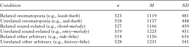
The main LMER analysis found a significant main effect of relatedness (ßunrelated = 0.07, p = < .001): judgement for related pairs was faster than for unrelated trials. There was also a significant main effect of duration (ß = 0.17, p < .001): longer auditory stimuli, not surprisingly, led to longer RTs. No other effects were significant. See Table 1 for descriptive statistics.
RT’s descriptive statistics (ms).

Similarly, the second analysis found a significant positive mean effect of duration (ß = 0.14, p < .001) on mean RT. But the relatedness effect was not significant. No other significant effect was found. See Tables 1 and 2 in the Supplementary Materials for full results.
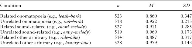
Accuracy’s descriptive statistics

3.1.2. Accuracy
In the first binary logistic regression, we found a significant main effect of relatedness (ßunrelated = 0.72, p < .001): participants were less accurate for related than unrelated pairs. No other significant effect was found. See Table 2 for descriptive statistics. The same negative effect of relatedness (ßunrelated = 0.77, p < .001) was also found in the second analysis, showing a consistent effect. No other main effect or interaction were significant. See Tables 3 and 4, supplementary materials, for full results.
3.2. EEG results
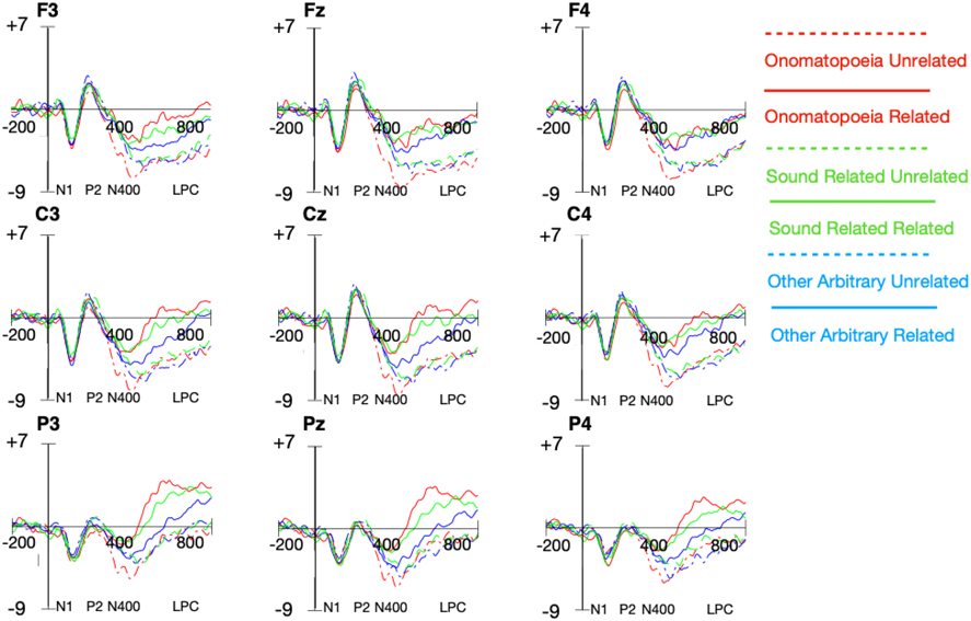
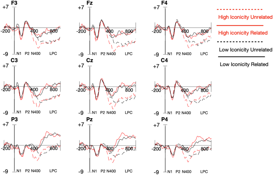
Figure 1 depicts the ERP responses for the nine electrodes analysed in the main analysis with condition as the predictor variable. Figure 2 shows the ERP response in the second analysis with iconicity as a predictor.
ERP plot of word type*relatedness in N1, P2, N400, and LPC. The plot was additionally filtered with a 30Hz low-pass filter for illustration.

ERP plot of iconicity*relatedness in N1, P2, N400, and LPC. The continuous variable iconicity was split into high and low iconicity categories for illustration only, each containing 30% highest and lowest iconicity words. The plot was additionally filtered with a 30Hz low-pass filter for illustration.

3.2.1. N1 (100–200 ms)
The first analysis suggested that unrelated items elicited more positive N1 (ßunrelated = 0.03, p < .001). Moreover, the comparison of the models with and without interaction terms was significant (p = .004). Follow-up analyses showed that the relatedness effect was significant for onomatopoeic (p < .001) as well as for other arbitrary words (p < .001), but not for sound-related words (p = .67). The negativity was more central-parietal distributed, as the frontal electrodes were less positive (ßfrontal = 0.04, p = .007). In the second analysis, we did not find the same effect of relatedness (ßunrelated = 0.04, p = .15) or interaction between iconicity and relatedness (ßunrelated:iconicity = 0.01, p = .56), but we found a significant effect of reaction time (ß = –0.03, p = .006). See full results and scalp distribution in Tables 5 to 7 and Figures 1 and 2, in the supplementary materials.
3.2.2. P2 (200–250 ms)
There was a significant relatedness effect in the first analysis of the P2 time-window: related items showed reduced positivity (ßunrelated = 0.02, p < .001). Duration also showed a significant effect (ß = –0.06, p = .006): longer words elicited less positive P2. There was no significant difference between models with and without the interaction term. The effect was mostly frontal, with frontal electrodes being more positive than central ones (ßfrontal = 0.04, p = .004), and parietal electrodes were less positive than central (ßparietal = –0.17, p < .001). P2 was strongest along the midline of the scalp, as both left-hemisphere electrodes (ßleft = –0.05, p = .001) and right-hemisphere electrodes (ßright = –0.042, p = .006) were less positive. The second analysis did not find any main or interaction effect involving relatedness or iconicity. With regard to control variables, P2 was less positive for words with a longer reaction time (ß = –0.02, p = .02) and duration (ß = –0.07, p = .03). The effect was more central-frontal distributed (ßparietal = –0.17, p < .001) compared with the frontal distribution in the initial analysis. But the effect was also strongest alone the midline, compared with both left hemisphere (ßleft = –0.06, p = .002) and right (ßright = –0.04, p = .02). See full results in Tables 8 and 9 and scalp distribution in Figures 3 and 4, in the supplementary materials.
3.2.3. N400 (300–500 ms)
There was a significant main effect of relatedness (ßunrelated = –0.06, p < .001) in the first analysis: unrelated pairs elicited a larger N400 than related pairs. Moreover, a models’ comparison showed a significant interaction (p < .001). The follow-up analysis showed that, for related pairs, the three word types were not significantly different. However, for unrelated pairs, onomatopoeic words were more negative than sound-related words (p = .01) and other arbitrary words (p = .05). There was no significant difference between the two arbitrary word groups (p = .70).
The N400 effect was mostly central, as both frontal (ßfrontal = 0.05, p = .001) and parietal (ßparietal = 0.08, p = .001) electrodes were less negative. The midline electrode was more negative than right hemisphere (ßright = 0.03, p = .02), but not the left hemisphere. This central-left distribution has been associated with auditory N400 (e.g., Hagoort & Brown, Reference Hagoort and Brown2000).
We found a clear N400 effect also in the second analysis, such that related items were significantly less negative (ßunrelated = –0.08, p = .001). There was also a significant interaction between relatedness and iconicity (ßunrelated:iconicity = –0.04, p = .03): N400 in unrelated trials was more negative for words with higher iconicity, thus confirming the results from the first analysis. With regard to the control variables, items with longer RT also elicited more negative N400 (ß = –0.04, p < .001). This effect was strongest in the central frontal electrodes compared with parietal (ßparietal = 0.09, p < .001). See full results in Tables 10 to 12, and scalp distribution in the supplementary materials, Figures 5 and 6.
3.2.4. LPC (600–900 ms)
The first analysis found a significant main effect of relatedness (ßunrelated = –0.15, p < .001): related pairs showed more positive LPC than unrelated. The models’ comparison showed a significant interaction (p = .02), but follow-up analysis did not find a significant difference between conditions in either related or unrelated trials. We also found that words with longer RT showed less positive LPC (ß = –0.10, p < .001). The positivity increased from frontal to parietal areas, central being more positive than frontal (ßfrontal = –0.10, p < .001), and parietal being more positive than central (ßparietal = 0.20, p < .001). The effect was strongest in the left hemisphere, as the left electrodes were more positive than the midline (ßleft = 0.04, p = .01), but midline and right electrodes were not significantly different.
The second analysis showed a significant main effect of relatedness (ßrelated = –0.17, p < .001), and a significant negative effect of RT (ß = –0.11, p < .001) in LPC. Frontal electrodes were less positive compared with central electrodes (ßfrontal = –0.11, p < .001), while parietal electrodes were more positive (ßparietal = 0.21, p < .001). The left hemisphere was more positive (ßleft = 0.04, p = .04). See full results in Tables 13 to 15, and scalp distribution in Figures 7 and 8, in the supplementary materials.
4. Discussion
Vocal iconicity has been argued to play a critical role during language evolution (e.g., Perlman, Dale, & Lupyan, Reference Perlman, Dale and Lupyan2015); it has been found to support language acquisition (e.g., Laing, Reference Laing2014), to render words more resistant after brain damage (Meteyard et al., Reference Meteyard, Stoppard, Snudden, Cappa and Vigliocco2015), and to facilitate processing also in healthy individuals (Reference Sidhu, Vigliocco and PexmanSidhu et al., this issue). It has also been shown that iconic words (onomatopoeic and mimetic words in Japanese) engage neural networks outside the typical language areas (to include right superior temporal sulcus (STS); Kanero et al., Reference Kanero, Imai, Okuda, Okada and Matsuda2014).
However, the current electro-physiological literature provides mixed results with respect to whether and when different brain signatures are found for iconic vs. arbitrary words. We have argued that this may be due in part to the use of typologically different languages that can be more or less rich in iconicity, differences in the class of iconic words being investigated, and, finally, differences in the tasks used that may not always fully engage semantic processing. Here we focused on onomatopoeia, the most direct and imitative form of iconicity (as it does not require any cross-modal mapping, which is typical instead of many cases of less direct iconicity as seen in mimetic words). Moreover, we focused on the semantic processing of these words using a task that explicitly required semantic processing (judging the semantic similarity between two words). The processing of onomatopoeic words was compared to the processing of more arbitrary words which in a critical condition also referred to sound (e.g., orchestra). Words in the three word classes were carefully matched for a number of psycholinguistic dimensions.
Across both behavioural and EEG data, not surprisingly, we found strong effects of relatedness with related pairs being processed faster and eliciting a reduced N400. We did not find differences between onomatopoeic and arbitrary words in RTs and accuracy. This result replicates what was found by Peeters (Reference Peeters2016) with onomatopoeia in Dutch in a lexical decision task. However, it should be noted that faster RTs (and more accurate responses) were reported in another study in English using onomatopoeia, also in a lexical decision task (Reference Sidhu, Vigliocco and PexmanSidhu et al., this issue). The reasons for this discrepancy are unclear as the languages are closely related, the three studies all focus on onomatopoeia, and whereas we used a semantic judgement task, the other two studies both used lexical decision (auditory presentation in Peeters, Reference Peeters2016, and visual presentation in Reference Sidhu, Vigliocco and PexmanSidhu et al., this issue).
Importantly, in our study we found electro-physiological differences in processing across the three word types in the N400 time-window (300–500 ms). More specifically, we found that the ERP elicited by correctly rejecting non-semantically related pairs was more negative for the onomatopoeic words than for both sound-related and other arbitrary words. The time-window and scalp distribution of the effect (maximal in centro-parietal electrodes) suggest that the effect is a genuine N400 (Kutas & Federmeire, Reference Kutas and Federmeier2011). The semantic processing of onomatopoeic words, thus, seems to differ from more arbitrary words, even if these words belong to the same semantic field (words referring to sound), in line with previous findings from Dutch (Peeters, Reference Peeters2016). We also found a relatedness effect for N1 and P2, with unrelated pairs eliciting more positive ERP in both time-windows, but only in the analysis with iconicity as a categorical variable and not in the analysis with iconicity as continuous variable. Similarly, there was a significant interaction in N1 between relatedness and iconicity, but only in the analysis with iconicity as a categorical variable (word type). It is unclear why we found these effects; however, as we observed them only in the analysis with iconicity coded as categorical (and not as a continuous variable), such effects could be driven by other (so far unknown) factors.
Finally, no effect was observed in the time-window for postlexical (LPC: 600–900 ms) processing driven by iconicity.
4.1. EEG signatures of iconicity
EEG studies investigating differences between onomatopoeic/mimetic words and arbitrary words, in principle, have the potential to identify differences in sensory, semantic, and postlexical processes and therefore provide a powerful tool for understanding how iconic words are processed. With regard to the sensory/phonological analysis of the words, we failed to observe consistent differences in early time-windows, in contrast to previous studies. Lockwood and Tuomainen (Reference Lockwood and Tuomainen2015) found differences between Japanese mimetic and arbitrary words in the peak of P2 (252–256 ms). Peeters (Reference Peeters2016) found differences in Dutch between onomatopoeic and arbitrary words in the N2 (150–200 ms) time-window (which overlapped with our N1 time-window). Lockwood and Tuomainen (Reference Lockwood and Tuomainen2015) explained the larger P2 for mimetic words as linked to phonological differences between mimetic and other words in terms of, especially, the reduplication of moras which is present in the mimetic but not in the other words considered in the study. Moreover, mimetic words are not restricted to auditory experience but can refer to all sorts of sensory experience, thus the P2 effect might also be linked to multimodal integration. In our study, we minimized any potential phonological difference between our onomatopoeic and control words, and no multimodal integration was required for the onomatopoeic words (as well as for the sound-related arbitrary words). More difficult is to account for the difference in results between our study and the study by Peeters (Reference Peeters2016). Not only was this study on a much closer language (Dutch), but also, just as in our study, he focused on onomatopoeia and presented auditory single words. Peeters observed more negativity in 150–200 ms for onomatopoeic than control words, which he attributes to the engagement of non-linguistic sound processing (in line with fMRI findings showing bilateral STS activations for mimetic words (Kanero et al., Reference Kanero, Imai, Okuda, Okada and Matsuda2014). However, this explanation does not take into account the fact that the fMRI findings refer to Japanese, where there are important phonology-related differences for mimetics. An important difference between Peeters (Reference Peeters2016) and our study is the task used. While Peeters used a lexical decision task, that may be argued to focus more on the form level; here we used a semantic decision task that forced participants to focus on semantics (and on the semantic relatedness between onomatopoeic and other words). This task was also a bit more difficult for our subjects, judging from their RTs (about twice as long as standard lexical decision RTs) and their error rates. One may speculate that lexical decision, by focusing more attention on word-form, may capture earlier correlates of iconicity (which indexes a transparent relation between word-form and meaning) than a task such as semantic decision, which instead focuses attention of meaning only.
Importantly, we found a clear difference between onomatopoeic and arbitrary words in the N400 window. More specifically, we found a difference between onomatopoeic and arbitrary words from different semantic classes, but also arbitrary words that, just like the onomatopoeic ones, evoke sound-related experiences (e.g., music). It has been shown in fMRI studies that sound-related (arbitrary) words activate networks involved in auditory perception (including posterior superior temporal gyrus/middle temoral gyrus; Kiefer et al., Reference Kiefer, Sim, Herrnberger, Grothe and Hoenig2008; Kiefer et al., Reference Kiefer, Trumpp, Herrnberger, Sim, Hoenig and Pulvermüller2012), indicating how, in general, words evoke associated sensory experience, in line with embodiment views of semantic representation (Barsalou, Reference Barsalou1999; Meteyard et al., Reference Meteyard, Cuadrado, Bahrami and Vigliocco2012). Onomatopoeic and sound-related arbitrary words should evoke similar sensory experience; however, special to onomatopoeic words is that such experience is part and parcel of the word-form. The larger N400 for onomatopoeic words was observed in the unrelated condition, which can be accounted for in terms of greater semantic activation for onomatopoeic words that then leads to increased dissimilarity with the cue. There was no complementary increase in positivity for the related condition. As most of our cue–target pairs in the onomatopoeic condition were not related on the basis of sound, whereas most of the pairs in the sound-related arbitrary word condition were, the lack of an effect for related pairs might be due to the fact that any enhancement of semantic activation for sound-related features (assumed to be greater for onomatopoeic words) is simply not relevant to the task as cue and target overlap in features other than sound (e.g., fingers–clap).
We did not observe any difference across word types in later time-window (600–900 ms, LPC), while, again we observed a strong effect of relatedness. As it is unclear whether the extent to which effects in this time-window are genuine or carry-over effects from the N400 time-window, and, moreover, there is no clear prediction for differences across word type in this time-window (which is considered to index postlexical decision processes), this result will not be discussed further.
4.2. proposed mechanisms for processing onomatopoeia
There are few accounts of how iconicity effects might come about in language processing (for a review, see Sidhu & Pexman, Reference Sidhu and Pexman2018). Many of these accounts cover not just onomatopoeia but the more general associations between specific phonemes and some general semantic features (e.g., the association of ‘i’ with smallness) and are based on associative mechanisms that can pick up such statistical correspondences. However, onomatopoeic words may be a special case. This is because they represent a unimodal type of iconicity (sounds in language mapping onto sounds in the world); they are extremely simple mappings (imitative) that do not require much learning; they appear to be universal across the world’s languages; and they feature heavily in the initial stages of language development.
Onomatopoeic words could be represented with mediated as well as direct links between word-form and semantic (sensorimotor) features. In standard connectionist architectures for spoken word recognition (e.g., McClelland & Elman, Reference McClelland and Elman1986), it is assumed that the link between phonological and semantic features is mediated via intermediate representations. It is argued that this mediation is necessary precisely to implement arbitrary relationships that cannot, otherwise, be learnt. However, onomatopoeia could have, in addition to mediated links, also direct connections between phonological/phonetic and semantic features: those that map in an imitative manner between the two levels. This proposal is consistent with the results of the present study: activation of semantic features is enhanced and this, in turn, renders a mismatch with an unrelated cue more salient (hence a larger N400). This account is also in line with the developmental evidence reviewed in the ‘Introduction’: direct mappings are easier to learn and therefore onomatopoeic words should be the first words being learnt (Laing, Reference Laing2014; Perry et al., Reference Perry, Perlman, Winter, Massaro and Lupyan2018; Thompson et al., Reference Thompson, Vinson, Woll and Vigliocco2012). According to this view, direct links would develop for onomatopoeic and not for other iconic words. Compatible with this is the finding by Reference Sidhu, Vigliocco and PexmanSidhu et al. (this issue) that facilitatory effects were found for onomatopoeic words, regardless of whether the task implicitly (lexical decision) or explicitly (phonological decision) recruited phonology, whereas facilitation was only found for other iconic words when the task explicitly recruited phonology.
A different mechanism that has been proposed in the literature for all iconic words (not just onomatopoeic words), is that their lexical representation encompasses both linguistic and non-linguistic sensory (sound-related in the case of onomatopoeia) features. This account has been put forward by Kanero et al. (Reference Kanero, Imai, Okuda, Okada and Matsuda2014) to account for bilateral activation of STS for mimetic but not arbitrary words. Our results can also be accounted for by this proposal. However, it is worth noting that a traditional divide between the processing of linguistic sounds in the left and the processing of non-linguistic sounds in the right hemisphere has been challenged (see, e.g., Schirmer, Fox, & Grandjean, Reference Schirmer, Fox and Grandjean2012).
4.3. conclusions
In the present paper, we have shown that making semantic judgements on onomatopoeic words vs. arbitrary words (including other words referring to sound) leads to processing differences as indexed by the N400. Crucially, by comparing the processing of onomatopoeia to a set of sound-related words, we could establish that any processing difference in this time-window for the onomatopoeic words cannot be accounted for in semantic terms only, but needs to take into account the special link between form and meaning that is present only in onomatopoeia.
Supplementary materials
For supplementary materials for this paper, please visit <http://doi.org/10.1017/langcog.2019.38>.