1. INTRODUCTION
Satellite-based Automatic Identification System (AIS) is providing a promising new aspect to maritime situational awareness, compared with traditional shore-based and vessel-based self-reporting systems. Satellite-based AIS can facilitate maritime traffic management and surveillance over a much longer range, and navigation and collision avoidance for vessels can be greatly enhanced with the assistance of satellite-based AIS. Since its introduction, many organisations have contributed to the development of relevant technologies, aiming to deploying a satellite constellation in order to accomplish a global coverage of vessels. It is estimated that a significant growth in AIS satellite constellations is due between 2012–2015 (Carson-Jackson, Reference Carson-Jackson2012). However, data collected by satellite-based AIS are often incomplete. Surface-based AIS reports and broadcasts have a range of around 35 miles. Satellite-based AIS has a much greater range, but may only receive portions of transmitted messages in a single orbit period, due to the limitations of its field of view and footprint. The loss rate of messages may also be high in regions of dense traffic. Therefore, data currently received by satellite-based AIS are essentially incomplete. How to make best use of this incomplete data to analyse vessels' behaviour from these data is an intriguing problem.
Determining the route of a single vessel of interest is important for surveillance, accident analysis and other purposes. Much work on this topic has been done using traditional shore-based and vessel-based AIS data. Peters and Hammond (Reference Peters and Hammond2011) determined the route of a vessel from two pieces of AIS messages using a probabilistic inference method. However, their proposed method constrains the vessel's maximum speed, making it only effective for long trips. In the process of generating random paths, the issue of computational efficiency may limit its application. Other problems for vessel tracking have also been studied. To reduce communication costs, a technique based on shared predictions between vessels and surrounding infrastructure is proposed to track the vessel with an accuracy guarantee (Redoutey et al., Reference Redoutey, Scotti, Jensen, Ray and Claramunt2008). This technique seems to assume that the surrounding stations can receive all reports broadcast by vessels, which, however, is not always true for satellite-based AIS. For multi-ship trajectory study in the context of collision avoidance, a method called “evolutionary sets of safe ship trajectories” has been developed (Szlapczynski, Reference Szlapczynski2011). This method can deal with two-ship and multi-ship encounter situations to help coordinate manoeuvres by analysing vessels' behaviour. In our work, situations involving multiple vessels are not considered. As for methods used for studying vessels' behaviour, there are also other strategies: the Bayesian network is used by Johansson (Reference Johansson and Falkman2007) and Mascaro (Reference Mascaro, Korb and Nicholson2010); a framework of adaptive kernel density estimation is proposed to perform the analysis of vessels' motion patterns in AIS data (Ristic, Reference Ristic, Scala, Morelande and Gordon2008) and a Gaussian mixture model is another strategy for statistical analysis of vessels' motion patterns in sea traffic (Laxhammar, Reference Laxhammar2008). More recently the latter two methods have been compared in detail by Laxhammar (Reference Laxhammar2009).
In this paper, by using a set of real incomplete AIS data received from the nano-satellite Tiantuo-1, designed by the National University of Defense Technology, we extracted the position (longitude and latitude), speed and course over ground (COG) information to perform vessel route inference in several situations. The Tiantuo-1 is a nano sized satellite orbiting in Low Earth Orbit (LEO). It carries an AIS receiver and collects messages transmitted by vessels at sea during its orbit. As its footprint has a limited coverage of vessels in each orbit period, collected data are essentially incomplete. However, with messages accumulated day by day, information on specific vessels in a region can be extracted. This is the raw data we will use in this paper and we set the time step to one day. The Maritime Mobile Service Identity (MMSI) identifies vessels and the dates when the messages are received are also recorded, taken from the temporal information in the AIS data.
The remainder of this paper is organised as follows: In Section 2, we establish the formulation of the problem and give the complete process of route inference for a single vessel. In Section 3, a real case study is presented and several situations are demonstrated to validate the proposed algorithm. A normalcy-checking algorithm is then detailed. In Section 4, we further discuss the results and the limitations of the algorithms. In Section 5, we conclude our work.
2. PROBLEM DESCRIPTION
The positions (longitude and latitude on a map) of a single vessel are denoted by a set of points Xi, (i=1,2,…,n_MMSI), where n_MMSI is the number of reports for the vessel identified by the MMSI code. For cases where no other information is available, the complexity of the vessel tracking problem would be to select one route from all possible
 $${\rm A}(n\_{\rm \smallcaps MMSI}) = n\_{\rm \smallcaps MMSI}!$$
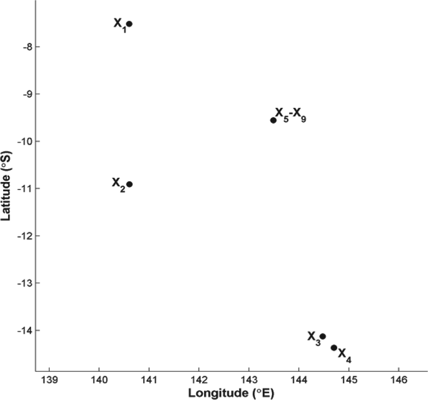
routes, each sequentially connecting all the n_MMSI position points without revisiting. However, as revisiting often occurs in real life, the primary model as formulated above is not sufficient for inference. In addition, taking a possible case as shown in Figure 1 for example, there could be coinciding positions reported on different time stamps, e.g. X5–X9, which in fact denotes being stationary, for example alongside or at anchor. This may be mistakenly explained as revisiting by the above model.
A set of position reports of a vessel scattered on the map, where X5–X9 coincide, which actually denotes remaining stationary in that position.

Due to limitations of the model established above, it is necessary to add other information to decrease the complexity. Of all the other information extracted from AIS messages, we then consider the time stamp pertinent to each message. This information can help determine the sequence in which a vessel passes by all its reported positions. Thus, we can easily distinguish between revisiting and remaining stationary. After adding the time information, the complexity of the problem expressed in Equation (1) is reduced directly. The result is shown in the left part of Figure 2.
Inference of a vessel's route using its position reports, the left with time stamp information added, and the right with speed and course over ground (COG) information added.
Further, the speed and COG information extracted from AIS messages are utilised to infer how the vessel travels past the reported positions in more detail. By investigating the magnitude of speed and its direction at each position, the skeleton of its route may be outlined. This is still coarse grained, as shown in the right part of Figure 2. Note that at X5–X9, the speed is zero, confirming that the vessel is staying there for 5 time units (5 days in this paper).
Next, the task of inference is to determine how to connect all the position points, satisfying all the constraints derived from the speed and COG information, i.e. to draw a route curve on which the velocity vector fits exactly the tangent at each reported position. In this paper, we present an inference strategy that can generate a feasible solution. The details are as follows:
At any position Xk, (k=1,2,…,  ${n}_{\underscore \rm \smallcaps MMSI^{-1}}$), the velocity vector is denoted by vk, the displacement vector connecting Xk and its successive position Xk+1 in the sequence by sk, and for convenience we scale sk to the same magnitude of vk,
 $${\bf s}_{\rm k} ' = |{\bf v}_{\rm k} |\times {\bf s}_{\rm k} /|{\bf s}_{\rm k} |$$
where |vk| and |sk| denote the magnitudes of corresponding vectors. In this paper, the time unit is a day, and the step size of inference is the distance that a vessel can cover in a day, which is
 $${\rm l}_{\rm k} = |{\bf v}_{\rm k} |\times {\rm t}$$
Two points should be noted. First, the speed decoded from raw AIS data has a unit of ‘knot’, where 1 kn=1·852 km/h. Here all the speeds are transformed to the unit of km/h. Correspondingly, t in Equation (3) equals to 24 h. Second, the accuracy of the step size is on the same level of that of the position information, as position reports are obtained on separate days.
When inferring the missing section between two successive positions Xk and Xk+1, we add a superscript index to the involved quantities for notation convenience, i.e. Xk(j), vk(j), sk(j), sk′(j), lk(j), (j=0,1,2,…). Then the direction, which is denoted by dk(j), from the current position to the next simulated position in one step of inference, is given by combining vk(j) and sk′(j). That is
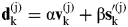 $${\bf d}_{\rm k} ^{({\rm j})} = {\rm \alpha} {\bf v}_{\rm k} ^{({\rm j})} + {\rm \beta} {\bf s}_{\rm k} '^{({\rm j})} $$
Here α and β are weight coefficients adjusting between vk(j) and sk′(j). Typically, we can set a constraint
 $${\rm \alpha} + {\rm \beta} = 1$$
for simplicity. So far, combining Equation (3), (4) and (5), we can get one new simulated position Xk(j+1) subsequent to Xk(j). Let
 $${\bf L}_{\rm k} ^{({\rm j})} = {\rm l}_{\rm k} ^{({\rm j})} \times {\bf d}_{\rm k} ^{({\rm j})} /|{\bf d}_{\rm k} ^{({\rm j})} |$$
and put the starting point of Lk(j) at Xk(j), then its end point denotes Xk(j+1), only to note that
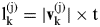 $${\rm l}_{\rm k} ^{({\rm j})} = |{\bf v}_{\rm k} ^{({\rm j})} | \times {\rm t}$$
In order to advance the iteration process to obtain a series of new simulated positions between Xk (assuming that Xk=Xk(0) initially) and Xk+1, we have to update two involved quantities at first, which are as follows:
 $$\eqalign{ & {\bf v}_{\rm k} ^{({\rm j} + 1)} = |{\bf v}_{\rm k} ^{({\rm j})} | \times {\bf d}_{\rm k} ^{({\rm j})} /|{\bf d}_{\rm k} ^{({\rm j})} | \cr & {\bf s}_{\rm k} ^{({\rm j} + 1)} = {\rm X}_{\rm k} ^{({\rm j} + 1)} \to {\rm X}_{{\rm k} + 1}} $$
Then the other quantities such as lk(j+1), sk′(j+1), dk(j+1), Lk(j+1) can be calculated accordingly. There are three points to be explained about Equation (8). First, in the initialization step, we set vk(0)=vk, sk(0)=Xk(0)→Xk+1 (i.e. Xk→Xk+1), where the superscript index starts from 0. Second, during each iteration between Xk and Xk+1, the magnitude of vk(j) never changes, while only its direction is being adjusted. This is because from the raw AIS data, we have no other complementary information to assist inferring its magnitude. Therefore, it is set to be constant until the algorithm converges to Xk+1. When the next loop of iterations beginning from Xk+1 is activated, it will be set as |vk+1|. Third, for the weight coefficients α and β, although we have constrained them in Equation (5), there is still some flexibility in assigning values. More intelligent strategies for assigning values for α and β can be used. However, for simplicity, we have used fixed values in this paper.
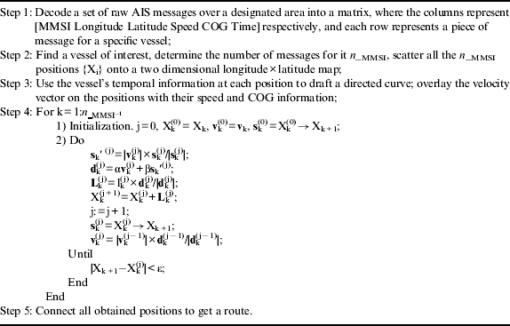
The process of detecting a vessel's route can now be summarised in Table 1.
Process of inferring intermediate positions of a specific vessel between reported positions, with the time step set to 1 day.
3. REAL CASE STUDY
In this section, we present a real case study with several different scenarios. Also, an algorithm that incorporates random deviations is given to expand the inferred route to a route band. This can validate the missing sections of obtained routes, and also detect anomaly behaviour for some scenarios. The region studied is a 50° Longitude×20° Latitude area to the north of Australia, as shown in Figure 3. The view in Figure 3 is produced by scattering the positions of all detected vessels over the period from 13 May 2012 to 7 October 2012 in this region. Note that there may be two categories of vessels in a region; one includes the local small vessels with or without AIS capability (see the congested dots along the coastal line), and the other includes the generally larger vessels sailing on the sea with AIS equipment (Hu et al., Reference Hu, Yong, Shi and Chen2010). In the subsequent research, we consider vessels whose AIS messages have been received by the satellite, no matter the category.
Scatter view of position information of all detected vessels in the region to the north of Australia, dating from 13 May 2012 to 7 October 2012.
3.1. Normalcy Validation
Even after finding intermediate positions between reported positions of a vessel on a possible route, it is still necessary to consider possible deviations. The quality and usage of AIS as a navigation tool needs a User Satisfaction Model to measure the degree of satisfaction and can be improved to some extent (Harati-Mokhtari et al., Reference Harati-Mokhtari, Brooks, Wall and Wang2007). This means that ignoring potential uncertainties in the data is not feasible. To account for inherent uncertainties, here we attempted to develop a route band in which the real route is most likely to be located. We further compare the behaviour of the vessel with that of surrounding vessels to validate its normalcy. If the normalcy checking is intensely violated, we can conclude that the vessel has taken part in illegal activities. In fact, from the perspective of a single vessel, it has to abide by traffic regulations or conventions at sea whatever its destination. Its velocity should be scheduled to some extent during the main section of its route, except for emergencies. From the overall regional perspective, sea routes follow generally predictable patterns and so cannot be randomly distributed. This can be seen from Figure 3. The route normalcy checking or validation is performed as follows.
3.2. Four Scenarios
In this subsection, we use the algorithm proposed in Section 2 to determine the routes of several different vessels, each representing a separate scenario. For the vessel demonstrated in Figure 1, its result is shown in Figure 4.
Route determination of a specific vessel (MMSI 503372000), utilising the method presented in Section 2. The left is a regional overall view with all detected surrounding vessels scattered for comparison. The right is the result of route determination.
In Figures 5–7, similar results are demonstrated for three other vessels, representing different scenarios.
The four results above are selected to demonstrate the applicability of the proposed algorithm to different scenarios. The first one in Figure 4 represents a scenario where the vessel is sailing onshore at first, then along a sealane, and lastly returns on another route. The second one in Figure 5 depicts a vessel loitering where there are no common vessel routes. This vessel may warrant examination, either for its own safety, or possible illegal activities. In Figure 6, the vessel is sailing mainly along a common route, yet it has changed its direction at some time. In Figure 7, there is a vessel heading for a destination from northwest at first, and then returning after some days. The algorithm proposed in this paper can deal well with all these scenarios. The number of AIS reports in each of these scenarios is less than 20.
Route determination of a specific vessel with MMSI 372636000.
Route determination of a specific vessel with MMSI 235073372.
Route determination of a specific vessel with MMSI 371707000.
3.3. Anomaly Detection
For the four scenarios, we further build up a passage or a band in which the routes we have determined can deviate, using a directly perceived technique given in Table 2. The results are demonstrated in Figure 8 respectively for each scenario. It can be seen that the routes (denoted in arrows) are all located within the band. For the first, third and fourth vessel, their bands fit the background traffic view on the whole. However, the second one demonstrates a closed “8”-shaped loitering behaviour. This process is judged visually by operators, and it may need some expert experience. However, this may assist in finding vessels needing help or in illegal activities.
Visual route bands of vessels in helping find anomaly behaviour. The second vessel (top right) seems to show anomalous behaviour.
Visual route normalcy checking process.

4. DISCUSSION
In the four scenarios, we used the proposed algorithm to infer the vessels' possible routes, and perform a normalcy analysis on them. Results show that the vessel in the second scenario (MMSI 372636000) seems to behave anomalously, while the other three vessels abide by corresponding background traffic patterns. The four scenarios were selected for particular reasons.
The first and third scenarios focus on vessels in coastal waters, the second focuses on a vessel in offshore waters, and the fourth focuses on a vessel making a round trip. These different scenarios represent typical behaviours of vessels, and the successful detection of their route patterns has validated the applicability of the algorithm presented in Table 1.
To alleviate the effect of uncertainties in the received AIS data, we have determined a route band in which the vessel's real route is most likely to be located. By comparing this band with the common routes formed by other vessels, we can determine the specific vessel's behaviour with more reliability.
The first, third and fourth vessels have travelled long distances, while the second one has been changing directions frequently in a small region. This behaviour can be interpreted from two aspects. On one hand, this vessel may need some help. On the other hand, it may be conducting illegal activities, such as illegal fishing. However, this should be verified by combining other information. For example, if it is fishing off-season for this region, more attention should be paid to this vessel because of its possible illegal activity.
However, there are still some points to be noted about the algorithm and the obtained results.
• Due to incompleteness of AIS data, route inference at turning corners (demonstrated by the background traffic view) is not very satisfactory, which can be seen from the right parts of Figures 4, 6 and 7, i.e. in the grid region at 142°–143° longitude×(−10°)–(−11°) latitude;
• In the fourth scenario, the vessel may be heading to a port and then returning. However, the supposed port is only denoted by the reported position which is nearest to it on the map, i.e. the one in the southeast corner of Figure 7. This is also due to data incompleteness;
• Error report screening is not considered in the algorithm. In fact, it is impossible to perform such a process here, for there is no supplementary information in the raw AIS data to assist. The reliability of the original data may be enhanced by technical design of the overall AIS system, which, however, is not considered in this paper;
• The analysis is ex post facto, not real time. With the development of AIS satellite constellations, when more satellites are deployed and more reports can be received, the algorithm could perform in real time, noting most of its limitations are due to data incompleteness;
• When determining the direction of a vessel, the information we use is the vessel's COG. A more complicated yet more reasonable consideration may involve both COG and true heading, where current flow effect can be well considered. For a sketchy inference, especially when data are incomplete, COG is sufficient;
• The judgement for anomaly behaviour needs some expert experience. The process and results shown in this paper only provide some clues.
Despite the limitations discussed above, in an early stage of data analysis of raw AIS reports received by satellite, especially when data are markedly incomplete, the method proposed in this paper can still give useful results for route determination and anomaly detection, as shown in the scenarios of Section 3.
5. CONCLUSION
In this paper, we have proposed an algorithm to infer the possible route of a vessel detected from incomplete satellite AIS data. The judgement of the vessel's anomalous behaviour has been made by comparing its route band with background traffic views visually, utilising expert experience. Analysing four typical scenarios in real case studies have validated the algorithm. From the obtained results, a vessel with possible anomalous behaviour has been identified and another three vessels are determined to be behaving normally. The limitations of the algorithm are also discussed in detail. Further work will be done to overcome these limitations, especially when the data are markedly incomplete.
ACKNOWLEDGMENTS
The authors would like to thank Mr. Lihu Chen and Yong Zhao for their kindness in acquisition of real data and message decoding.