



1 Introduction
Liquid curtains, i.e. vertical liquid sheets free-falling in a gaseous atmosphere, are of practical interest for many applications, amongst which are surface coating (Miyamoto & Katagiri Reference Miyamoto and Katagiri1997) and paper manufacturing (Soderberg & Alfredsson Reference Soderberg and Alfredsson1998). Their dynamics and stability, and more generally that of all liquid sheets, is a longstanding problem that has been the concern of numerous experimental and theoretical studies. In the late 1950s, Taylor (Reference Taylor1959a
) showed that an obstacle across a liquid sheet creates two types of capillary waves: varicose (or symmetric) waves, which induce thickness modulations and are dispersive; and sinuous (or antisymmetric) waves, which induce a displacement of the sheet mid-plane and are non-dispersive in the long-wavelength limit. He also determined the criterion for the steady recession of a free edge, that is, for the existence of a steady hole in the sheet (Taylor Reference Taylor1959b
): the edge of a liquid sheet with thickness
 $h$
, surface tension
 ${\it\sigma}$
and density
 ${\it\rho}$
recedes with a velocity
 $\sqrt{2{\it\sigma}/{\it\rho}h}$
, at which the capillary stresses balance the inertia of the liquid collected at the edge. When this receding velocity equals that of the flow perpendicular to the edge, the edge location is steady. Brown (Reference Brown1961) used this criterion to determine the stability to rupture of a steady curtain, in which the flow is accelerated by gravity and the sheet thins downstream. The most critical direction is the recession against the flow, in the upward vertical direction, for which the steadiness of the flow requires that the local Weber number of the sheet is equal to one, that is,
 $$\begin{eqnarray}\displaystyle \mathit{We}=\frac{{\it\rho}hw^{2}}{2{\it\sigma}}=1, & & \displaystyle\end{eqnarray}$$
where
 $w$
is the local velocity in the curtain. For
 $\mathit{We}\leqslant 1$
the flow is subcritical: any hole forming in the curtain expands in all directions. This has a particular consequence for a free-falling liquid curtain in which, by contrast with other sheet flows such as axisymmetric liquid sheets (see e.g. Taylor Reference Taylor1959a
; Clanet Reference Clanet2007; Villermaux, Pistre & Lhuissier Reference Villermaux, Pistre and Lhuissier2013),
 $\mathit{We}$
increases in the downstream direction due to the acceleration of the flow. A hole forming in an unperturbed curtain at a location where
 $\mathit{We}\leqslant 1$
therefore expands upstream until the whole of the curtain is disrupted. We will see below that this is not necessarily true for a perturbed curtain. Note also that the criterion (1.1), which holds for a straight and steady weightless edge, is modulated by the shape of the edge (Gordillo, Lhuissier & Villermaux Reference Gordillo, Lhuissier and Villermaux2014), its acceleration (Lhuissier & Villermaux Reference Lhuissier and Villermaux2011) and gravity (Roche et al.
Reference Roche, Le Grand, Brunet, Lebon and Limat2006).
This criterion on the criticality of the flow only concerns the fate of the curtain once a hole has formed, but not the actual stability of a curtain, which also depends on the occurrence of puncturing events. This is indeed a common observation (see e.g. Finnicum, Weinstein & Ruschak (Reference Finnicum, Weinstein and Ruschak1993) and Le Grand et al. (Reference Le Grand, Brunet, Lebon and Limat2006), or more evidently the direct observation of a static soap film) that a liquid curtain can be maintained at
 $\mathit{We}<1$
. In practical situations, these puncture events often result from boundary effects or defects that are present in the flow (Dombrowski & Fraser Reference Dombrowski and Fraser1954; Lhuissier & Villermaux Reference Lhuissier and Villermaux2013). For large-velocity liquid sheets, the puncture is also triggered by the flapping motion (Kelvin–Helmholtz like instability) due to the shear with the quiet gaseous atmosphere around the sheet (Squire Reference Squire1953; Dombrowski & Fraser Reference Dombrowski and Fraser1954). Several studies (Lin, Lian & Creighton Reference Lin, Lian and Creighton1990; De Luca & Costa Reference De Luca and Costa1997; Teng, Lin & Chen Reference Teng, Lin and Chen1997; Weinstein et al.
Reference Weinstein, Clarke, Moon and Simister1997) considered this mechanism in the context of free-falling liquid curtains. They recovered that, for a thin liquid sheet, the flapping instability only develops for a local Weber number of the sheet larger than one, when the velocity of the wave is smaller than that of the flow (Squire Reference Squire1953). This means that, for a free-falling liquid curtain, perturbations are expected to grow only over the downstream part of the curtain where they are advected by the flow (convective instability). An algebraic growth of perturbations due to the non-parallel structure of the flow has also been predicted (De Luca & Costa Reference De Luca and Costa1997), the role of which in the puncturing of a liquid curtain has not however been experimentally demonstrated.
To gain insight into the dynamics and puncturing mechanisms of the sheet, studying the response of a liquid sheet to an imposed perturbation has proved to be a useful method. Following Taylor (Reference Taylor1959a ), who used a single small air jet blowing against a liquid sheet to study the sinuous and varicose capillary wakes, numerous works considered the linear capillary response to different local perturbations: obstacle across the curtain (Lin & Roberts Reference Lin and Roberts1981), non-contact electrostatic periodic forcing (Clarke et al. Reference Clarke, Weinstein, Moon and Simister1997) or acoustic forcing in the presence of a gaseous atmosphere (Soderberg & Alfredsson Reference Soderberg and Alfredsson1998). Within this limit of linear capillary waves, Alleborn & Raszillier (Reference Alleborn and Raszillier2004) incorporated the influence of the viscous damping on local varicose perturbations. By contrast, finite-amplitude perturbations have received much less attention. They have only been considered numerically on the one-dimensional configuration of a liquid sheet perturbed by air blades by Mehring & Sirignano (Reference Mehring and Sirignano2003), who identified the ratio of the stagnation pressure of the air to that of the liquid as the relevant parameter for rupture. Besides these localized perturbations, let us note that global perturbations have been considered: static pressure applied on one side of a curtain (Finnicum et al. Reference Finnicum, Weinstein and Ruschak1993) or stabilization of the shear-induced flapping instability by an air co-flow (Tammisola et al. Reference Tammisola, Sasaki, Lundell, Matsubara and Söderberg2011). However, as far as we know, large-amplitude localized perturbations in a two-dimensional curtain, both varicose and sinuous, which can have either dramatic local effects or effects manifesting far downstream of the perturbation, have not been considered.
In the present study, we thus address the question of the response of a curtain to a local perturbation with finite amplitude. Inspired by Taylor’s (Reference Taylor1959a ) small air jet, we apply a controlled perturbation with either one pulsed air jet or two steady air jets blowing perpendicularly against the curtain. This lets us vary both the shape (symmetric or asymmetric), the strength and the time scale of the perturbation, and reveals a rich dynamics. Asymmetric pulsed perturbations either deform, fragment, puncture or inflate the curtain in bubbles, while steady symmetric perturbations allow for the steady opening of the curtain at a controllable distance from the perturbation.
The paper is organized as follows. Section 2 introduces the experimental set-up. Section 3 presents our observations of the various response regimes induced by pulsed asymmetric perturbations and of the steady hole that forms downstream of a steady symmetric perturbation. A model for this latter regime of symmetric perturbation is presented in § 4. It is compared to the experiments in § 5, and a conclusion is given in § 6.
2 Experimental set-up
The experimental set-up allows for the formation of a vertical steady liquid curtain on which a controlled localized perturbation can be applied. It is sketched in figure 1. The same Newtonian liquid was used for all the experiments: silicone oil (Dow Corning DC200) with density
 ${\it\rho}=957~\text{kg}~\text{m}^{-3}$
, kinematic viscosity
 ${\it\nu}=50~\text{mm}^{2}~\text{s}^{-1}$
and surface tension
 ${\it\sigma}=20.4~\text{mN}~\text{m}^{-1}$
. The oil is pumped at constant flow rate
 $Q$
, measured with a variable-area flowmeter, to a feeding chamber consisting of a hollow aluminium cylinder with horizontal axis. The curtain is formed by forcing the liquid throughout a 2 mm wide and 155 mm long rectangular slit cut on the upper part of the cylinder. At the slot exit, the liquid flows down, on both sides, over the cylinder outer surface that it wets entirely. For sufficiently large flow rate, the liquid forms a flat vertical curtain at the bottom of the cylinder – for low flow rates, the liquid detaches in drops or forms columns (Pritchard Reference Pritchard1986; Giorgiutti, Limat & Weisfreid Reference Giorgiutti, Limat and Weisfreid1995; Brunet, Flesselles & Limat Reference Brunet, Flesselles and Limat2007). To prevent the lateral shrinking of the curtain, the latter is guided on both sides by vertical wires to which it remains attached. The curtain is ended at its bottom by the surface of a shallow pool of the same liquid, into which it falls. From this pool, the liquid gently flows into a collecting tank, from where it is pumped back through the circuit, which gives a continuous operation of the system. This set-up provides a stable rectangular curtain, with a width
 $L=155$
mm and a height of
 $435$
mm, with a purely vertical perturbation-free flow. The dynamics of the applied perturbation was visualized with a high-speed camera (IDT N3).
A flat vertical liquid curtain is formed by letting silicone oil fall uniformly from the bottom of a horizontal aluminium cylinder. At a distance
 $z_{0}$
below the bottom of the cylinder, a localized perturbation with controlled amplitude is applied by blowing air perpendicularly against the curtain.

The vertical velocity
 $w(0)$
at the top of the curtain (i.e. at the bottom of the cylinder at
 $z=0$
) is only a few millimetres per second, that is to say, much smaller than the typical velocity downstream in the curtain, which is of the order of
 $1~\text{m}~\text{s}^{-1}$
. Moreover, neither surface tension nor viscosity significantly affects the base flow, since both the capillary length
 $\sqrt{{\it\sigma}/{\it\rho}g}\simeq 1.5~\text{mm}$
, over which a capillary slowdown is expected, and the visco-gravity length
 ${\it\nu}^{2/3}g^{-1/3}\simeq 0.6~\text{mm}$
, over which a viscous slowdown is expected (Brown Reference Brown1961), are much shorter than the distances
 $z>2~\text{cm}$
to the top of the curtain that are considered here (quantitatively, their combined influence on the velocity is always smaller than 4 %). In the absence of perturbations, the liquid in the curtain thus practically experiences a free-fall with velocity
 $$\begin{eqnarray}\displaystyle w=\sqrt{2gz}. & & \displaystyle\end{eqnarray}$$
The curtain is steady, and its thickness
 $h={\it\Gamma}/w$
is everywhere proportional to the flow rate per unit width
 ${\it\Gamma}=Q/L$
, which we obtain from the measurement of the global flow rate
 $Q$
. The unperturbed thickness thus decreases in the downstream direction, according to
 $$\begin{eqnarray}\displaystyle h=\frac{{\it\Gamma}}{\sqrt{2gz}}. & & \displaystyle\end{eqnarray}$$
In our experiments,
 ${\it\Gamma}$
ranges from typically 0.5 to
 $5~\text{cm}^{2}~\text{s}^{-1}$
, and the typical unperturbed thickness
 $h$
of the curtain is of the order of 10–
 $100~{\rm\mu}\text{m}$
. The local Weber number in the curtain thus increases with increasing distance
 $z$
to the slit according to
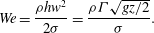 $$\begin{eqnarray}\displaystyle \mathit{We}=\frac{{\it\rho}hw^{2}}{2{\it\sigma}}=\frac{{\it\rho}{\it\Gamma}\sqrt{gz/2}}{{\it\sigma}}. & & \displaystyle\end{eqnarray}$$
Once a steady liquid curtain has formed, a local perturbation is applied at a distance
 $z_{0}$
below the top of the curtain, which we vary between typically 1 and 10 cm. The perturbation is achieved by blowing air from small pipes perpendicularly against the curtain. Two types of perturbations were applied: pulsed asymmetric perturbations, and steady symmetric perturbations. In the former case (see figure 2
a), only one pipe is used and the air flow is pulsated with a pulse duration
 $T$
. In the latter case (figure 2
b), two coaxial pipes are located symmetrically with respect to the curtain and each of them blows the same steady air flow. The size of the perturbation is directly set by the pipes’ inner radius
 $r_{a}=2.5~\text{mm}$
, since the pipes’ outlets are located close (5 mm) to the liquid curtain. We checked that from 2 to 6 mm the pipe–curtain distance does not affect the phenomena under study: the shape and strength of the perturbation are invariant over the considered range. The pipes radius, hence the size of the perturbation, was kept constant for all the experiments. By contrast, the amplitude of the perturbation, which is set by the flow rate
 $Q_{a}$
feeding each air jet, was systematically varied. The air flow is created by pressurizing air, with density
 ${\it\rho}_{a}=1.18~\text{kg}~\text{m}^{-3}$
and kinematic viscosity
 ${\it\eta}_{a}=1.85\times 10^{-5}~\text{Pa}~\text{s}$
, and regulating the flow in the jets with a pressure-reducing valve. The volume flow rate in each jet
 $Q_{a}$
is measured with a variable-area flowmeter located upstream of the pipes. It was varied between 30 and
 $140~\text{cm}^{3}~\text{s}^{-1}$
, which corresponds to typical air velocities
 $v_{a}=Q_{a}/{\rm\pi}r_{a}^{2}$
ranging from 1.5 to
 $7~\text{m}~\text{s}^{-1}$
and typical stagnation pressures
 ${\it\rho}_{a}v_{a}^{2}/2$
ranging from 1.5 to 30 Pa. For pulsed jets, a solenoid on–off valve controlled by a low-frequency generator with square signal was added to the circuit after the flowmeter. It allowed for the blowing on demand with a desired pulse duration and a strength set by the flow rate
 $Q_{a}$
, which was measured when the on–off valve is opened.
The advantage of this set-up is its ability to control the strength, the duration and to some extent the shape of the perturbation.
-
(1) When a single pipe blows (figure 2 a), the perturbation is asymmetric. The liquid is mainly deflected transversely and the mid-plane of the curtain is displaced.
-
(2) When the two facing pipes blow with the same strength (figure 2 b), the liquid is deflected only in the plane of the curtain, and the curtain thins symmetrically.
Two types of localized perturbation are applied to the curtain. (a) Asymmetric non-steady perturbation: a single pulsed air jet blows for a duration
 $T$
with a repetition rate
 $(2T)^{-1}$
. (b) Symmetric steady perturbation: two identical jets, facing each other on both sides of the curtain, blow continuously.

For the sake of generality, rather than using
 $Q_{a}$
, which depends strongly on the choice of the pipe radius, we will discuss all the experiments in terms of the mean air velocity in the jet, that is to say,
 $v_{a}=Q_{a}/{\rm\pi}r_{a}^{2}$
.
3 Observations
3.1 Pulsed asymmetric perturbations: various regimes of instabilities
When the curtain was subjected to a pulsed air jet from a single side, we observed different regimes of response depending on the flow parameters. The experiments were conducted as follows. We set the height of the perturbation to
 $z_{0}$
, which imposes the vertical velocity of the liquid on the jet axis
 $w_{0}=\sqrt{2gz_{0}}$
, and varied both the flow rate per unit width
 ${\it\Gamma}$
and the air velocity
 $v_{a}$
(when the on–off valve is opened). The air pulses had a duration
 $T$
ranging from 25 to 50 ms. For the sake of a clear identification of the different regimes, the pulses were repeated periodically with a frequency
 $(2T)^{-1}$
. However, the time between successive pulses was always much larger than the characteristic time of the flow advection over the jet size
 $2r_{a}/w_{0}$
, which varied between 3 and 8 ms over the range of
 $z_{0}$
we considered. Except for the largest air velocities (regime (vi) below), each pressure pulse was thus independent of the others and, without loss of generality, the response of the curtain can be considered as that to an isolated pressure pulse with duration
 $T$
. The induced deformation generally consists of both a local displacement of the sheet perpendicular to its plane and a local thinning of the sheet. For weak perturbations (
 $v_{a}$
typically smaller than
 $3.5~\text{m}~\text{s}^{-1}$
), the curtain response showed smooth wavy deformations. For stronger air blows, however, spectacular and potentially destructive dynamics were observed, which we present later.
For low flow rates, the upper part of the curtain, where the local Weber number
 $\mathit{We}={\it\rho}{\it\Gamma}\sqrt{2gz}/2{\it\sigma}$
is smaller than 1, is metastable. Providing the external perturbations are weak enough, it is possible to maintain a stable curtain for some time. However, when a localized perturbation with sufficient amplitude is applied in the upper part, the curtain punctures and the hole extends over the whole curtain, which results in the global disruption of the latter. Figure 3 shows the early stage of this disruption when the Weber number on the jet axis (
 $z=z_{0}$
) is
 $\mathit{We}_{0}=0.93$
. The hole propagates in all directions and eventually covers the whole curtain. This situation with a metastable unperturbed state is drastically sensitive to external noise and to the curtain downstream boundary conditions, since sinuous perturbations can propagate upstream, and we thus focused on stable unperturbed states.
Response to a pulsed asymmetric perturbation for a low liquid flow rate (
 ${\it\Gamma}=0.38~\text{cm}^{2}~\text{s}^{-1}$
,
 $z_{0}=5.5~\text{cm}$
,
 $T=50~\text{ms}$
and
 $v_{a}=5.91~\text{m}~\text{s}^{-1}$
). The images in the sequence are taken 4, 10, 16, 32 and 70 ms after the first one and their height represents
 $6.5~\text{cm}$
. A bulge is formed which inflates and eventually punctures. The resulting hole propagates both downstream and upstream (c–e) which causes the disruption of the entire curtain (f).

Response to the same asymmetric perturbation as in figure 3 for a larger flow rate (
 ${\it\Gamma}=1.27~\text{cm}^{2}~\text{s}^{-1}$
,
 $z_{0}=5.5~\text{cm}$
,
 $T=50~\text{ms}$
and
 $v_{a}=5.91~\text{m}~\text{s}^{-1}$
). The images in the sequence are taken 14, 20, 26, 32, 48 and 86 ms after the beginning of the air pulse, and their height represents
 $6.5~\text{cm}$
. A bulge is formed which also punctures but, by contrast with figure 3, the resulting hole is only intermittent. While it grows, the hole is advected downstream by the steady flow, and the curtain self-heals.

For larger flow rates (
 ${\it\Gamma}>2{\it\sigma}/{\it\rho}\sqrt{2gz_{0}}$
), the response to the perturbation always develops downstream of the jet. Figure 4 illustrates this point in the case when the jet punctures the curtain. By contrast with the situation in figure 3, the resulting hole is only intermittent: while the hole grows, it is advected downstream by the flow and the curtain self-heals. For these large flow rates, not only holes but also very different regimes of curtain response were observed, the limits of which depend not only on the jet velocity
 $v_{a}$
but also on the flow rate
 ${\it\Gamma}$
and position
 $z_{0}$
. All of these regimes can, for instance, be observed for a fixed flow
 ${\it\Gamma}=2~\text{cm}^{2}~\text{s}^{-1}$
in the middle of the range of interest. By progressively increasing
 $v_{a}$
from 0 to
 $8~\text{m}~\text{s}^{-1}$
, the following response regimes were observed.
Periodic ejection of droplets and bubbles observed for a repeated pulsed asymmetric perturbation with large amplitude (
 ${\it\Gamma}=2.01~\text{cm}^{2}~\text{s}^{-1}$
,
 $z_{0}=5.5~\text{cm}$
and
 $T=25~\text{ms}$
). (a) Air velocity
 $v_{a}=5.61~\text{m}~\text{s}^{-1}$
. The height of the images is
 $6.5~\text{cm}$
. The air blows form liquid filaments at the crest of high-amplitude waves that break up into droplets. (b) Air velocity
 $v_{a}=6.04~\text{m}~\text{s}^{-1}$
. The blows distort the curtain and inflate bubbles that eventually detach. (c) Superposition of successive images separated by 50 ms showing the bubbles’ ejection dynamics in the same conditions as in (b).

-
(i) A narrow wake downstream of the perturbation, similar to that observed downstream of any wetting obstacle inserted across a curtain (Taylor Reference Taylor1959a ; Lin & Roberts Reference Lin and Roberts1981).
-
(ii) High-amplitude sinuous waves that first bulge on the opposite side of the jet and eventually oscillate and dampen downstream, without puncturing or fragmenting the curtain.
-
(iii) The ejection of liquid filaments from the crests of the wave, which eventually fragment into droplets (see figure 5 a).
-
(iv) The ejection of bubbles, which detach from the curtain when the inflated bulges pinch off (see figures 5 b,c).
-
(v) Intermittent holes, which are formed by the puncturing of the bulges before a bubble detaches and are subsequently advected by the flow (see figure 4).
-
(vi) A single permanent hole, with a triangular edge pointing in the upstream direction, resulting from the connection of the intermittent holes. Close to the transition with the intermittent holes regimes, the edge position oscillates strongly, a few centimetres downstream of the jet. Obviously, in this regime, the pulses are not isolated from each other and their repetition rate becomes a relevant quantity.
Note that in the regimes (i)–(iv), including when droplets and bubbles are ejected, no hole forms in the curtain, even transiently. It must also be mentioned that both the droplet and bubble sizes (typically 1 and 5 mm, respectively) were highly reproducible.
Figure 6 presents the phase diagram of the curtain responses described above. It shows the boundaries, in terms of the dimensionless flow rate in the curtain
 ${\it\rho}{\it\Gamma}/{\it\rho}_{a}r_{a}\sqrt{2gz_{0}}$
and the dimensionless mean velocity in the jet
 $v_{a}/\sqrt{2gz_{0}}$
, between the different regimes (i)–(vi) for
 $z_{0}=5.5~\text{cm}$
and a pulse duration
 $T=25~\text{ms}$
. Below
 ${\it\Gamma}\simeq 0.5~\text{cm}^{2}~\text{s}^{-1}$
(that is to say,
 ${\it\rho}{\it\Gamma}/{\it\rho}_{a}r_{a}\sqrt{2gz_{0}}\simeq 15$
), which is close to the critical value
 $2{\it\sigma}/{\it\rho}\sqrt{2gz_{0}}\simeq 0.44~\text{cm}^{2}~\text{s}^{-1}$
, the curtain response is not reproducible. Above this flow rate, the response regimes (i)–(vi) are observed and, for a given location
 $z_{0}$
, all the thresholds in the perturbation strength between them increase with increasing curtain flow rate.
Providing a detailed modelling of these thresholds, which rely on several destabilization mechanisms (pinch-off and hole nucleation), is clearly beyond the scope of the present study. We however simply note that the transverse displacement of the curtain induced by the air jet (over the time
 $r_{a}/w_{0}$
it interacts with each portion of the curtain) is expected to be typically
 ${\it\rho}_{a}v_{a}^{2}r_{a}^{2}/{\it\rho}{\it\Gamma}w_{0}$
. This transverse displacement forms a significant bulge, from which a bubble, a drop or a hole may result, when it becomes of the order of
 $r_{a}$
, that is to say, when
 $v_{a}/w_{0}\sim \sqrt{{\it\rho}{\it\Gamma}/{\it\rho}_{a}r_{a}w_{0}}$
. This heuristic criterion of a ‘significant’ transverse displacement defines the threshold (dashed line) shown in figure 6. Somewhat surprisingly, although it ignores all the details of the mechanisms of the different regimes, this criterion reproduces the order of magnitude as well as the general trend of the threshold between regimes (v) and (vi), for the formation of a permanent hole.
Phase diagram of the different regimes of response to a pulsed asymmetric perturbation (
 $z_{0}=5.5$
cm,
 $T=25~\text{ms}$
) in terms of the dimensionless flow rate in the curtain
 ${\it\rho}{\it\Gamma}/{\it\rho}_{a}r_{a}\sqrt{2gz_{0}}$
and the dimensionless mean velocity in the air jet
 $v_{a}/\sqrt{2gz_{0}}$
. The lines show the delimitations between the different regimes. The dashed line shows the limit
 $y=\sqrt{x}$
, above which the transverse displacement of the curtain is expected to become larger than the size of the perturbation (see text).

3.2 Steady symmetric perturbations
We now turn to the curtain response to a symmetric perturbation: a local thinning imposed by two steady air jets facing each other on both sides of the curtain (figure 2 b). The jets locally squeeze the curtain and generate a smooth varicose perturbation with a controlled amplitude set by the air velocity (the jets actually also generate a tenuous sinuous wake, which can be observed under a raking lighting (see figure 12), but the latter does not affect the puncture of the curtain).
Figure 7 shows the typical curtain response. For a sufficiently strong air flow, the perturbation forms a steady hole at some distance downstream of the jets. The hole is bounded by a steady liquid edge receding against the flow. This free edge has the shape of an inverted V with a round top, and the hole extends downstream to the bottom of the curtain (see figure 7). This shape is similar to those obtained by inserting a non-wetting obstacle across a liquid curtain (Brown Reference Brown1961; Lin & Roberts Reference Lin and Roberts1981; Roche et al. Reference Roche, Le Grand, Brunet, Lebon and Limat2006), except that the upstream portion of the edge is round instead of being angular. This difference is of crucial importance. It results from the fact that, in the present case, the location of the edge is not prescribed by that of the obstacle, but is actually selected by the flow of the curtain and the strength of the perturbation: the steadiness and the symmetry of the flow, together with the absence of an obstacle that can impart momentum, impose the condition that, exactly downstream of the jets, the edge be locally horizontal.
Steady hole created in the liquid curtain downstream of a symmetric perturbation for increasing flow rates
 ${\it\Gamma}=2.01,~2.25,~2.48,~2.71,~2.94$
and
 $3.17~\text{cm}^{2}~\text{s}^{-1}$
from (a) to (f). Here
 $z_{0}=1.15~\text{cm}$
and
 $v_{a}=3.97~\text{m}~\text{s}^{-1}$
. The height of the images is
 $11.8~\text{cm}$
. The hole moves downstream (the distance
 $z_{e}$
–
 $z_{0}$
from the jets to the upstream edge of the hole increases) with increasing flow rates
 ${\it\Gamma}$
. The white disk in (a) shows the location and the size of the perturbation.

The distance
 $z_{e}-z_{0}$
from the hole upstream edge to the jets globally decreases with decreasing flow rates and increasing jet velocity. For large flow rates, this distance remains almost constant, fluctuating by a few per cent only due to the small irregularities of the flow. By contrast, within a narrow range of flow rate, when
 ${\it\Gamma}$
is just above the threshold for global rupture, the location of the free edge fluctuates greatly, sometimes erratically, sometimes with a periodic motion (with a typical frequency of a few hertz). During this motion, the free edge conserves a constant shape, with only slight variations in its aperture angle. Although the origin of these fluctuations is still open to question, they are reminiscent of those reported by Roche et al. (Reference Roche, Le Grand, Brunet, Lebon and Limat2006), who observed the oscillations of a free edge generated by a non-wetting obstacle inserted across a curtain at
 $\mathit{We}\simeq 0.7$
. Note also that the aperture angle of the free edge decreases with increasing flow rate, as expected for a free edge receding steadily in a unperturbed free-falling liquid curtain (Brown Reference Brown1961).
We also checked that no hysteresis was present in the process by alternately decreasing and increasing both the air flow rate and the curtain flow rate. Once a hole has formed, both methods were reversible, and yielded the same measurements. This total reversibility of the phenomenon is actually in agreement with direct observations showing that the location and the shape of the hole directly result from the thickness modulations generated by the jets. These modulations are clearly visible in figure 7, through the optical distortion of the background pattern positioned behind the curtain. These distortions are confined to a rather narrow wake downstream of the jets, the width of which slowly decreases with increasing flow rate. Figure 8 shows a close-up view of the distortions, from which the main features of the modulated thickness field can be deduced. As expected, the wake is symmetric with respect to the
 $z$
axis. In each horizontal cross-section downstream of the jets (A–A in figure 8), the thickness is reduced and essentially uniform over a large part of the wake around the axis. This central thinner part is bounded on both sides by ridges of greater thickness which connect to the unperturbed thickness field outside the wake. This thickness profile is confirmed by the shape of the film edge, which is almost horizontal over most of the wake width, highly curved at the ridges where the thickness changes significantly, and straight with a constant inclination outside the varicose wake.
Figure 9 shows the variation of the hole location
 $z_{e}$
with the mean air jet velocity
 $v_{a}$
and the curtain flow rate
 ${\it\Gamma}$
for different vertical locations of the jets:
 $z_{0}=2.05$
cm (a),
 $z_{0}=4.6$
cm (b) and
 $z_{0}=9.1$
cm (c). To the best of our knowledge, this is the first time that it has been shown that a local perturbation on a curtain induces the formation of a steady free edge further downstream in a reproducible fashion and at a controllable distance from the perturbation. This is however clearly reminiscent of air jet-induced dewetting used for cleaning and drying substrates (Berendsen, Zeegers & Darhuber Reference Berendsen, Zeegers and Darhuber2013).
Details of the symmetrical wake and the steady hole from figure 7(c). (a) The optical distortion of the black and white stripes in the background highlights the thickness modulations in the wake. (b) Typical thickness profile upstream (A–A) and downstream (B–B) of the hole inferred from the optical distortion. In A–A, the wake consists of a thinner sheet portion with almost uniform thickness, bordered by two ridges.

Location
 $z_{e}$
of the upstream edge of the hole versus the curtain flow rate
 ${\it\Gamma}$
, for different jet velocities
 $v_{a}$
(indicated in the legend) and different locations of the perturbation indicated by the dashed lines: (a)
 $z_{0}=2.05~\text{cm}$
, (b)
 $z_{0}=4.6~\text{cm}$
and (c)
 $z_{0}=9.1~\text{cm}$
.

4 Model for a steady symmetric perturbation
We now present a model for the steady thinning and opening of the liquid curtain in the wake of the perturbation in the case of facing jets. In the experiments, the thinning results from both the motion imparted by the air jets and the acceleration imparted by gravity. However, these contributions are independent of each other and other situations might occur where gravity is irrelevant. For the sake of clarity, we will thus focus in this section on the sole contribution of the air blows, while the contribution of gravity will be readily incorporated in § 5.
(a) Radial pressure profile (solid line) and radial shear profile (dashed line), (4.1) and (4.2) respectively, due to the air blow at the curtain surface. (b) Schematics of the influence of the pressure and shear on the curtain in the present case when the jets diameter is much larger than the sheet thickness.

4.1 Stresses between the jets
We therefore consider for now a flat liquid sheet with uniform thickness
 $h_{0}$
and vertical velocity
 $w_{0}\boldsymbol{e}_{\boldsymbol{z}}$
that is perturbed by two air jets, symmetric with respect to the sheet mid-plane and blowing perpendicularly against the sheet. These jets create an initial perturbation of typical size
 $r_{0}$
, which evolves downstream in the form of a stationary wake, while it is advected by the main flow (see figures 7 and 8). The perturbation of the liquid sheet actually results from two concomitant forces at the air/liquid interface, at the point where the air jets impact the sheet perpendicularly, that is to say (see figure 10):
-
(1) the stagnation pressure due to the deflection of the air parallel to the plane of the sheet, which builds up on the jets axis;
-
(2) the shear stress, due to the tangential air flow resulting from the jets’ deflection, which is largest immediately around the jets axis.
As we will discuss below, both forces are important in experiments, and need to be considered. We model the air pressure by the following radial profile centred on the jet axis:
 $$\begin{eqnarray}\displaystyle p=p_{0}\exp \!\left(-\frac{x^{2}+(z{-}z_{0})^{2}}{r_{0}^{2}}\right). & & \displaystyle\end{eqnarray}$$
Here
 $p_{0}$
and
 $r_{0}$
respectively represent the stagnation pressure on the jet axis and the typical size of the pressure profile, which can be readily related to the velocity profile of the air jets, that is to say, to
 $v_{a}$
and
 $r_{a}$
(see appendix A). This choice for the profile is dictated by two considerations. First, it is physically relevant both on the axis, where the pressure profile is known to be locally parabolic (Schlichting Reference Schlichting1979), and over larger radii, where the pressure vanishes. As we will see, this permits one to quantitatively consider the dynamics of thinning in the high- and low-Reynolds-numbers limits, respectively. Second, this simple profile can be quantitatively connected to the air jet velocity profiles (see appendix A) and permits analytical calculations that reveal the mechanism and the limits of the model. Following the classical analysis for the boundary layer development around the axis of a fluid jet impacting perpendicularly on a solid surface (Schlichting Reference Schlichting1979), the shear stress
 ${\it\tau}\boldsymbol{e}_{\boldsymbol{r}}$
at the air/liquid interface (the liquid velocity being negligible with respect to the air velocity) can be expressed as
 $$\begin{eqnarray}\displaystyle & & \displaystyle \frac{{\it\tau}}{-r_{0}\partial _{r}p}\simeq 1.312\left(\frac{{\it\eta}_{a}^{2}}{2{\it\rho}_{a}p_{0}r_{0}^{2}}\right)^{1/4}\equiv \frac{{\it\tau}_{0}}{p_{0}}.\end{eqnarray}$$
Here
 ${\it\rho}_{a}$
and
 ${\it\eta}_{a}$
respectively stand for the density and the dynamic viscosity of air, and
 $r$
is the radial coordinate centred on the jets axis. Note that (4.2) is strictly valid close to the jets axis only, over a typical size
 $r_{0}$
. For simplicity, we assume in the following that it is also valid further from the axis, although the precise shape of the shear profile there is of little importance, since the evolution of the perturbation and the formation of the hole are dictated by the conditions close to the axis.
The size
 $2r_{0}\sim 5~\text{mm}$
of the perturbation is much larger than the thickness
 $h_{0}\sim 50{-}500~{\rm\mu}\text{m}$
, and the pressure is thus essentially uniform across the sheet. Moreover, the time scale
 $h_{0}^{2}/4{\it\nu}\sim 1~\text{ms}$
for the diffusion of momentum across the liquid is much smaller than the typical time scale
 $\mathscr{T}\sim 10~\text{ms}$
of the sheet dynamics. The shear stress at the air/liquid interface therefore also readily transmits to the whole thickness. This has two important consequences. First, the liquid velocity is essentially uniform across the thickness, which means that the dynamics is accurately described by a slender slope model that only considers the local thickness
 $h$
and the average velocity
 $\{u,w\}$
across the sheet. Second, anticipating (4.5), the resultant of the air pressure and that of the air shear on a sheet portion respectively can be expressed as
 $-h\partial _{r}p\boldsymbol{e}_{\boldsymbol{r}}$
and
 $2{\it\tau}\boldsymbol{e}_{\boldsymbol{r}}$
. Since, from (4.2),
 ${\it\tau}\propto -\partial _{r}p$
, this means that, as long as the thickness is uniform, the contribution of the shear stress is everywhere proportional to that of the pressure. We thus define the effective pressure
 $$\begin{eqnarray}\displaystyle P_{0}=p_{0}+\frac{2r_{0}{\it\tau}_{0}}{h_{0}}, & & \displaystyle\end{eqnarray}$$
which accounts for both contributions. The ratio
 $h_{0}p_{0}/2r_{0}{\it\tau}_{0}\sim ({\it\rho}_{a}p_{0}/{\it\eta}_{a}^{2}r_{0}^{2})^{1/4}h_{0}$
of the two terms shows that, not surprisingly, the contribution of the shear is larger for thin sheets than for thicker ones.
Last, we make use of the observation that the lateral velocity
 $u\boldsymbol{e}_{\boldsymbol{x}}$
induced by the perturbation is much smaller than the vertical velocity of the unperturbed flow
 $w_{0}\boldsymbol{e}_{\boldsymbol{z}}$
that advects the perturbation. That is, the wake is elongated and varies only slowly along
 $\boldsymbol{e}_{\boldsymbol{z}}$
. We thus introduce the small parameter
 ${\it\varepsilon}\sim u/w_{0}$
, which we will define precisely further down, and describe the wake as a one-dimensional perturbation evolving along
 $\boldsymbol{e}_{\boldsymbol{x}}$
only, while it is advected along
 $\boldsymbol{e}_{\boldsymbol{z}}$
. In the frame of reference of a sheet portion moving at
 $w_{0}\boldsymbol{e}_{\boldsymbol{z}}$
, the (effective) air pressure now has the form of a pressure pulse,
 $$\begin{eqnarray}\displaystyle P=P_{0}\exp \!\left(-\frac{x^{2}+(w_{0}t)^{2}}{r_{0}^{2}}\right), & & \displaystyle\end{eqnarray}$$
where
 $t=\int _{z_{0}}^{z}\text{d}z/w_{0}$
stands for the time since a portion of the sheet has passed at the height of the jets. The velocity
 $u$
and thickness
 $h$
then satisfy
 $$\begin{eqnarray}\displaystyle & \displaystyle \partial _{t}u+u\partial _{x}u=\frac{4{\it\nu}\partial _{x}(h\partial _{x}u)}{h}-\frac{\partial _{x}p}{{\it\rho}}+\frac{2{\it\tau}\boldsymbol{e}_{\boldsymbol{r}}\boldsymbol{\cdot }\boldsymbol{e}_{\boldsymbol{x}}}{{\it\rho}h}, & \displaystyle\end{eqnarray}$$
 $$\begin{eqnarray}\displaystyle & \displaystyle \partial _{t}h+\partial _{x}(uh)=0, & \displaystyle\end{eqnarray}$$
which can be derived from the general two-dimensional equation given in appendix B by keeping the dominant terms for
 $u/w\sim {\it\varepsilon}\ll 1$
and
 $x\sim r_{0}\sim {\it\varepsilon}z$
and subsequently substituting
 $\text{d}z=w_{0}\,\text{d}t$
. Note that, in deriving (4.5), we set the pressure in the sheet equal to the pressure
 $p$
in the air, that is, we neglected the Laplace pressure arising from the curvature of the air/liquid interface, as we will justify below.
4.2 Impulsive acceleration between the jets
A crucial consequence of
 $u\ll w$
is that, for a portion of liquid flowing across the pressure field imposed by the air jets, the time
 $r_{0}/w_{0}$
during which the pressure is applied is much shorter than the typical time
 $r_{0}/u$
over which the perturbation evolves. We therefore consider, from now, the relevant limit case in which the perturbation is given by an impulsive pressure pulse. This implies that, immediately after the pulse, the sheet is still undeformed (
 $h=h_{0}$
), but it has acquired a velocity
 $$\begin{eqnarray}\displaystyle u(x,0)=\int _{-\infty }^{\infty }\frac{-\partial _{x}p+(2{\it\tau}/h_{0})\boldsymbol{e}_{\boldsymbol{r}}\boldsymbol{\cdot }\boldsymbol{e}_{\boldsymbol{x}}}{{\it\rho}}\,\text{d}t, & & \displaystyle\end{eqnarray}$$
as follows from neglecting both the advective term
 $u\partial _{x}u\sim {\it\varepsilon}\partial _{t}u$
and the viscous term
 $4{\it\nu}\partial _{x}(h\partial _{x}u)/h\sim {\it\varepsilon}({\it\nu}/ur_{0})\partial _{t}u$
in (4.5) and neglecting
 $\partial _{x}(uh)\sim {\it\varepsilon}\partial _{t}h$
in (4.6).
Moreover, since in this impulsive limit the air shear and the air pressure apply on a curtain with uniform thickness, the velocity can be directly expressed in terms of the effective pressure
 $P_{0}$
defined in (4.3), that is
 $$\begin{eqnarray}\displaystyle u(x,0)=2\sqrt{{\rm\pi}}\frac{P_{0}}{{\it\rho}w_{0}}\frac{x}{r_{0}}\exp \!\left(-\frac{x^{2}}{r_{0}^{2}}\right). & & \displaystyle\end{eqnarray}$$
This point is crucial, as it implies that the same model can be used to describe the wake for all cases: when the pressure is dominant, when the shear is dominant, or when both terms are of comparable magnitude. Only the expression and the magnitude for
 $u$
are changed, but not the shape of the wake.
From (4.8), one readily sees that the typical ratio
 $u/w$
, which we assumed to be small, is actually set by the parameter
 $$\begin{eqnarray}\displaystyle {\it\varepsilon}\equiv \frac{P_{0}}{{\it\rho}w_{0}^{2}}. & & \displaystyle\end{eqnarray}$$
This parameter has two influences that cannot be decoupled in the present configuration, i.e. that of a sheet flowing between stationary air jets. As already mentioned, it sets both the relative time span of the pressure pulse, and the typical angle of the wake
 ${\sim}u/w_{0}$
. Therefore, a small value of
 ${\it\varepsilon}$
justifies both the assumption of our one-dimensional model and that of the limit case of an impulsive pressure pulse. Last, it is also important to realize that the vertical velocity is essentially not influenced by the air pressure. Indeed, in the case of an impulsive pressure pulse, one has
 $w(x,0)=-\!\int _{-\infty }^{\infty }P_{z}\,\text{d}t/{\it\rho}=0$
, while the corrections for a finite
 ${\it\varepsilon}$
are of the order of
 ${\it\varepsilon}^{2}$
only (at the first order, the vertical deceleration upstream of
 $z_{0}$
is exactly balanced by the acceleration downstream). For a free-falling liquid curtain, the vertical velocity
 $w$
thus only varies because of the acceleration imparted by gravity, but remains
 $x$
-independent, which will be used for modelling the wake downstream.
4.3 Modulated thickness wake
After (i.e. downstream of) this impulsive acceleration, the forcing of the jets vanishes and the dynamics of the sheet depends at the first order on inertia and viscous dissipation, as one can see by setting
 $p=0$
and
 ${\it\tau}=0$
in (4.5). By making use of the characteristic velocity
 $P_{0}/{\it\rho}w_{0}$
and the size scale
 $r_{0}$
of (4.8), together with the inertial time scale
 $r_{0}/u$
, which is formed by the ratio of the former to the latter, namely
 $$\begin{eqnarray}\displaystyle \mathscr{U}=\frac{P_{0}}{{\it\rho}w_{0}},\quad \mathscr{X}=r_{0},\quad \mathscr{T}=\frac{{\it\rho}r_{0}w_{0}}{P_{0}}, & & \displaystyle\end{eqnarray}$$
equations (4.5) and (4.6) can be written in dimensionless form as
 $$\begin{eqnarray}\displaystyle & \displaystyle \partial _{t}u+u\partial _{x}u=\frac{1}{h}\partial _{x}\!\left(\frac{h\partial _{x}u}{\mathit{Re}}\right), & \displaystyle\end{eqnarray}$$
 $$\begin{eqnarray}\displaystyle & \displaystyle \partial _{t}h+\partial _{x}(uh)=0, & \displaystyle\end{eqnarray}$$
where we have introduced the Reynolds number
 $$\begin{eqnarray}\displaystyle \mathit{Re}=\frac{r_{0}P_{0}}{4{\it\nu}{\it\rho}w_{0}}. & & \displaystyle\end{eqnarray}$$
This Reynolds number, which ranges from 0.35 to 2.3 in the experiments, depends on the thickness only through the air shear at the interface. It is otherwise set by the size
 $r_{0}$
of the perturbation. Therefore, in the case of a pressure-dominated motion, the whole dynamics is independent of the initial thickness
 $h_{0}$
. This dynamics deforms the air/liquid interface and one may also expect a dependence on
 $h_{0}$
due to surface tension, as in the case studied by Taylor (Reference Taylor1959a
). However, in our experiments the Laplace pressure is of the order of
 ${\it\sigma}h_{0}/r_{0}^{2}$
, that is, less than one-tenth of the air effective pressure
 $P_{0}$
. Surface tension is thus negligible at the impact of the air jets.
Thickness evolution in the wake for a curtain with parallel flow (
 $w=w_{0}$
). (a) Thickness profiles at
 $t/\mathscr{T}=0.1,0.2,0.4$
and 0.6 for the purely inertial limit (
 $\mathit{Re}\gg 1$
). (b) Thickness profiles at
 $t/\mathscr{T}=0.05,0.2,0.8$
and 3.2 for the viscous limit (
 $\mathit{Re}\ll 1$
) plotted for a Reynolds number of
 $\mathit{Re}=0.5$
. (c) Evolution of the thickness on the centreline for the inertial solution (4.16) (red) and for the viscous solution (4.23) with
 $\mathit{Re}=0.1,0.3,$
and 0.9 (black).

In the scales of (4.10a-c ), the velocity after the pulse is simply
 $$\begin{eqnarray}\displaystyle u(x,0)=2\sqrt{{\rm\pi}}x\,\text{e}^{-x^{2}}. & & \displaystyle\end{eqnarray}$$
4.3.1 Inertial thinning
It is instructive first to consider the case of a high Reynolds number. In this case the sheet portions simply propagate (along
 $\boldsymbol{e}_{\boldsymbol{x}}$
) with a constant velocity, which is given by their initial position
 $x$
. Defining respectively
 $X(x,t)=x+u(x,0)t$
and
 $H(x,t)$
as the Lagrangian coordinate and thickness of the film portions, mass conservation yields
 $$\begin{eqnarray}\displaystyle H=\frac{h_{0}}{\partial _{x}X}=\frac{h_{0}}{1+\partial _{x}u(x,0)t}. & & \displaystyle\end{eqnarray}$$
This corresponds to the thickness profiles shown in figure 11(a). As time increases, a central thinner portion, bordered by thicker ridges propagating outwards at a constant velocity, develops. Its thickness, which at
 $x=0$
where
 $u=0$
is equal to the Eulerian thickness, evolves as
 $$\begin{eqnarray}\displaystyle h(0,t)=\frac{h_{0}}{1+2\sqrt{{\rm\pi}}t}. & & \displaystyle\end{eqnarray}$$
Therefore, in the absence of viscosity, the impulsive acceleration generates a wake in which the sheet thins down to zero over an infinite distance.
It is also worthwhile to look further from the vertical of the jets (
 $z$
axis). As it propagates outwards, the initial velocity wave deforms until it develops a shock (assuming an infinite Reynolds number). This shock forms when the inflection point of the curve, which also propagates at a constant velocity, straightens down to adopt an infinite negative slope (see figure 11
a). This occurs at the time and distance from the axis given by
 $$\begin{eqnarray}\displaystyle & \displaystyle t_{c}=\frac{\text{e}^{3/2}}{4\sqrt{{\rm\pi}}}\simeq 0.63, & \displaystyle\end{eqnarray}$$
 $$\begin{eqnarray}\displaystyle & \displaystyle x_{c}=\left(\frac{3}{2}\right)^{3/2}\simeq 1.84, & \displaystyle\end{eqnarray}$$
above which (4.16) is a priori no longer valid, since viscosity has necessarily come into play at some point before the singularity occurs.
However, before invoking viscosity, it is crucial to realize the following point: the viscous term in (4.11) identically vanishes on the axis (at
 $x=0$
). This means that the thinning dynamics on the axis, which ultimately determines whether or not the curtain will puncture, will be the last portion of the wake where viscous effects will modify the thickness profile (4.15) (the first one being the location of the singularity at the edges of the wake). It is therefore likely that the result of (4.16) will be almost unchanged until the Reynolds number becomes fairly close to one.
Illustration of the evolution of the local Weber number in the jets wake. (a) A thin rod (white arrow) is inserted across the liquid curtain close to the varicose wake (not visible here) generated by the main perturbation (the air jets are pointed out by the white disk, and the height of the image represents
 $16.1~\text{cm}$
). The deflection in the steady sinuous wake of the rod reveals the thickness modulations in the main wake. (b) The local orientation
 ${\it\theta}$
of the rod wake is a measurement of the local Weber number
 $\mathit{We}=1/\sin ^{2}{\it\theta}$
. The horizontal portion of the wavefront (red dashed arrow), on the wake axis, thus reveals that the flow is critical there (
 $\mathit{We}=1$
), that is, at a short distance upstream of the steady edge of the hole.

4.3.2 Viscous thinning
It is also possible to describe the dynamics for the opposite limit of a small Reynolds number (i.e.
 ${\it\varepsilon}\ll \mathit{Re}\ll 1$
). In that case, (4.8) remains valid while (4.11) simplifies to the diffusion equation
 $$\begin{eqnarray}\displaystyle \partial _{t}u=\frac{1}{h}\partial _{x}\left(\frac{h\partial _{x}u}{\mathit{Re}}\right)\simeq \frac{\partial _{xx}u}{\mathit{Re}}, & & \displaystyle\end{eqnarray}$$
since
 $h\simeq 1$
. This equation has an exact well-known solution (see e.g. Fourier Reference Fourier1822, p. 470) that matches the initial condition
 $u(x,0)$
from (4.14), that is,
 $$\begin{eqnarray}\displaystyle u(x,t)=2\sqrt{{\rm\pi}}\frac{x}{(1+4t/\mathit{Re})^{3/2}}\exp \!\left(-\frac{x^{2}}{1+4t/\mathit{Re}}\right), & & \displaystyle\end{eqnarray}$$
which yields the velocity gradient on the axis,
 $$\begin{eqnarray}\displaystyle \partial _{x}u(0,t)=2\sqrt{{\rm\pi}}\frac{1}{(1+4t/\mathit{Re})^{3/2}}. & & \displaystyle\end{eqnarray}$$
Within the same approximation as in (4.19), mass conservation becomes (the approximation being actually exact on the axis)
 $$\begin{eqnarray}\displaystyle \partial _{t}h=-\partial _{x}(hu)\simeq -h\partial _{x}u, & & \displaystyle\end{eqnarray}$$
which together with (4.21) gives the dimensionless thickness on the
 $z$
axis,
 $$\begin{eqnarray}\displaystyle \frac{h(0,t)}{h_{0}}=\exp \!\left[-\sqrt{{\rm\pi}}\mathit{Re}\left(1-\frac{1}{\sqrt{1+4t/\mathit{Re}}}\right)\right]. & & \displaystyle\end{eqnarray}$$
Note that not only the thickness on the axis, but also the whole thickness field,
 $$\begin{eqnarray}\displaystyle \frac{h(x,t)}{h_{0}}=\exp \!\left[-\sqrt{{\rm\pi}}\mathit{Re}\left(\text{e}^{-x^{2}}-\frac{\text{e}^{-x^{2}/(1+4t/\mathit{Re})}}{\sqrt{1+4t/\mathit{Re}}}\right)\right], & & \displaystyle\end{eqnarray}$$
is known, which is shown in figure 11(b). Interestingly, (4.23) shows that, in the absence of a restoring force and in contrast with the inertial case, the relative thickness downstream of the jets converges to a finite value
 $$\begin{eqnarray}\displaystyle \frac{h}{h_{0}}\rightarrow \text{e}^{-\sqrt{{\rm\pi}}\mathit{Re}} & & \displaystyle\end{eqnarray}$$
after a typical time
 $$\begin{eqnarray}\displaystyle t\sim \frac{\mathit{Re}}{4}, & & \displaystyle\end{eqnarray}$$
as illustrated in figure 11(c).
5 Connection with experiments
The previous model considered an unperturbed flow with uniform velocity (i.e.
 $w=\text{cte}$
). It is readily connected to the case of a gravity-driven liquid curtain, for which the velocity
 $w$
and the unperturbed thickness
 $h_{0}$
now depend on the height according to (2.1) and (2.2).
Indeed, as we have already mentioned, the vertical velocity
 $w$
is not affected at first order by the air blows, the contribution of which is simply to delay any sheet portion passing between them: the air jets first slow the flow down (while it is still upstream) and then accelerate it back (downstream of the pipe). Second, the stretching imposed by gravity along
 $\boldsymbol{e}_{\boldsymbol{z}}$
and that induced by the blows along
 $\boldsymbol{e}_{\boldsymbol{x}}$
are perpendicular to each other. This means that, at first order, both effects will contribute to the thinning of the sheet multiplicatively: hence one can use (4.16) and (4.23) for
 $h/h_{0}$
directly with the free-fall velocity and thickness from (2.1) and (2.2), that is,
 $$\begin{eqnarray}\displaystyle h=\frac{{\it\Gamma}}{w}\times \frac{h}{h_{0}}\bigg|_{w=w_{0}}. & & \displaystyle\end{eqnarray}$$
To determine the puncture of the curtain in the wake of the air jets, we now need to express the criterion for the existence of a steady hole. Since we discuss the cases when a hole is observed, we can disregard the nucleation of the hole itself (that is, the possibility of a metastable but steady subsonic flow) to consider only the condition for a steady free edge in the sheet. The opening of the hole is most favourable (the hole opens faster) on the axis of the wake, where the sheet is thinner. As we have already mentioned, the limiting direction is that of the edge portion propagating vertically, against the flow. Following Taylor (Reference Taylor1959b
) and Culick (Reference Culick1960), and considering the weight
 ${\it\rho}g{\rm\pi}d^{2}/4$
of the rim at the edge, where
 $d\simeq 1~\text{mm}$
stands for the rim diameter, the momentum conservation at the edge (where it is perpendicular to both the main velocity
 $w\boldsymbol{e}_{\boldsymbol{z}}$
and gravity) imposes the condition that
 $$\begin{eqnarray}\displaystyle {\it\rho}hw^{2}+{\it\rho}g{\rm\pi}d^{2}/4=2{\it\sigma}, & & \displaystyle\end{eqnarray}$$
that is to say, a condition on the sole local Weber number of the flow,
 $$\begin{eqnarray}\displaystyle \mathit{We}=\frac{{\it\rho}hw^{2}}{2{\it\sigma}}=\mathit{We}_{c}\equiv 1-\frac{{\rm\pi}{\it\rho}gd^{2}}{8{\it\sigma}}\simeq 0.8. & & \displaystyle\end{eqnarray}$$
This value is consistent with the typical values of 0.7 observed in previous experiments by Roche et al. (Reference Roche, Le Grand, Brunet, Lebon and Limat2006). Making use of (2.1) and (2.2), this criterion can also be expressed as
 $$\begin{eqnarray}\displaystyle \frac{{\it\rho}{\it\Gamma}}{{\it\sigma}}\sqrt{\frac{gz}{2}}\frac{h}{h_{0}}\bigg|_{w=w_{0}}=\mathit{We}_{c}. & & \displaystyle\end{eqnarray}$$
If we now consider the inertial thinning (4.16), we obtain in physical units
 $$\begin{eqnarray}\displaystyle \frac{{\it\rho}{\it\Gamma}}{{\it\sigma}}\sqrt{\frac{gz}{2}}\frac{1}{1+2\sqrt{{\rm\pi}}t/\mathscr{T}}=\mathit{We}_{c}, & & \displaystyle\end{eqnarray}$$
where the time
 $t$
since the film portion has passed between the jets, expressed in terms of the distance
 $z$
, is
 $$\begin{eqnarray}\displaystyle t=\int _{z_{0}}^{z}\frac{1}{w}\,\text{d}z=\sqrt{\frac{2z}{g}}-\sqrt{\frac{2z_{0}}{g}}. & & \displaystyle\end{eqnarray}$$
Hence the criterion in terms of the location
 $z_{e}$
of the edge is
 $$\begin{eqnarray}\displaystyle \mathit{We}_{0}\sqrt{\frac{z_{e}}{z_{0}}}=\mathit{We}_{c}\left[1+2\sqrt{{\rm\pi}}\frac{P_{0}}{{\it\rho}gr_{0}}\left(\sqrt{\frac{z_{e}}{z_{0}}}-1\right)\right], & & \displaystyle\end{eqnarray}$$
where
 $\mathit{We}_{0}={\it\rho}{\it\Gamma}\sqrt{2gz_{0}}/2{\it\sigma}$
is the non-perturbed Weber number at the location of the jets, from which
 $z_{e}$
can be readily expressed as
 $$\begin{eqnarray}\displaystyle \frac{z_{e}}{z_{0}}=\left(\frac{{\it\alpha}-1}{{\it\alpha}-\mathit{We}_{0}/\mathit{We}_{c}}\right)^{2},\quad \text{with }{\it\alpha}=2\sqrt{{\rm\pi}}\frac{P_{0}}{{\it\rho}gr_{0}}. & & \displaystyle\end{eqnarray}$$
Let us note that, since
 ${\it\alpha}>0$
, a stable hole can exist downstream of the perturbation if and only if
 ${\it\alpha}>(1+\mathit{We}_{0}/\mathit{We}_{c})/2>1$
. Otherwise, the whole of the wake is supersonic, hence unconditionally stable. Interestingly, in this limit, the local Weber number on the axis tends towards a finite value. This is because at long times the thinning (due to both gravity and the air blows) exactly compensates the gravitational acceleration of the flow, which results in a constant momentum
 ${\it\rho}hw^{2}$
. Furthermore, note that, in the case of inertial thinning, one always has
 $\partial _{z}\mathit{We}\leqslant 0$
along the axis of the wake. This means that if a hole forms (
 $\mathit{We}<\mathit{We}_{0}$
), the edge will reach a stable location, in contrast with the usual case of an unperturbed free-falling liquid curtain (for which
 $\partial _{z}\mathit{We}\geqslant 0$
), where a hole is either advected by the flow or disrupts the whole curtain.
This scenario is supported by direct observations reported in figure 12, which qualitatively but unambiguously illustrate the spatial evolution of the local Weber number
 $\mathit{We}$
in the wake of the jets. It relies on the observation of the sinuous wake generated by a thin and wetted rod inserted across the curtain that plays the role of a probe. The local angle of the rod sinuous wake with respect to the vertical
 ${\it\theta}$
relates to the local Weber number according to
 $\mathit{We}=1/\sin ^{2}{\it\theta}$
(Brown Reference Brown1961). By adequately positioning the rod, one can visualize the variation of
 $\mathit{We}$
in the wake of the jets. The horizontal portion of the rod wake (shown by a red dashed arrow in figure 12
b) thus reveals the location where
 $\mathit{We}=1$
. By moving the rod and probing different locations in the jets wake, we could check that, by contrast with the usual trend in the absence of perturbation given by (2.3), the Weber number indeed decreases with increasing distances to the jets
 $(z-z_{0})$
. This confirms why the edge location is stable (
 $\partial _{z}\mathit{We}<0$
). We could also check that no steady wave could propagate close to the hole upstream edge: when the rod is slightly displaced downstream from its position in figure 12, the path of its sinuous wake abruptly jumps downstream to the hole edge. This shows that
 $\mathit{We}$
is everywhere smaller than 1 down to the hole edge (see figure 12
b), in agreement with our assumption of
 $\mathit{We}\simeq 0.8$
at the edge.
For the sake of completeness, let us remark that the criterion
 $\mathit{We}=\mathit{We}_{c}$
in (5.4) can also be used together with (4.23) to obtain a closed relation for the edge location in the case of a viscosity-limited thinning (
 $\mathit{Re}\ll 1$
), i.e.
 $$\begin{eqnarray}\displaystyle \mathit{We}_{0}\sqrt{\frac{z_{e}}{z_{0}}}=\mathit{We}_{c}\exp \!\left[\sqrt{{\rm\pi}}\mathit{Re}\left(1-\frac{1}{\sqrt{1+{\displaystyle \frac{4{\it\alpha}}{\mathit{Re}}}\left(\sqrt{{\displaystyle \frac{z_{e}}{z_{0}}}}-1\right)}}\right)\right], & & \displaystyle\end{eqnarray}$$
which, by contrast with the inertial case, cannot be reduced to an explicit expression for
 $z_{e}$
.
Comparison between the theoretical model for an inviscid curtain (
 $\mathit{Re}=\infty$
) and the experiments. The prediction for the location of the stationary free edge
 $z_{e}/z_{0}$
is plotted against the actual value (the black line is the prediction). The blue circles show the experiments for which the assumptions of the model apply (large Reynolds number
 $\mathit{Re}>0.5$
and narrow wakes
 ${\it\varepsilon}=P_{0}/{\it\rho}w_{0}^{2}>0.1$
), while the red squares show all the other experiments.

Returning to (5.8), i.e. in the situation when viscosity is negligible, the model yields a quantitative prediction for the location of the hole. Figure 13 compares the theoretical prediction for an infinite Reynolds number (black line) to all the experiments (disks), for which
 $2.05~\text{cm}<z_{0}<9.1~\text{cm}$
,
 $0.67~\text{cm}^{2}~\text{s}^{-1}<{\it\Gamma}<4.48~\text{cm}^{2}~\text{s}^{-1}$
and
 $1.84~\text{m}~\text{s}^{-1}<v_{a}<6.14~\text{m}~\text{s}^{-1}$
. All the experimental trends are captured at least qualitatively by the model: the threshold value for the jets velocity, the decrease of
 $z_{e}/z_{0}$
with increasing jets velocity and decreasing flow rates, and the stability of the hole location. However, not surprisingly, the quantitative agreement is good only for those data in blue (circles), for which both the Reynolds numbers are sufficiently large (
 $\mathit{Re}>0.5$
) and the wakes are sufficiently narrow (
 ${\it\varepsilon}=P_{0}/{\it\rho}w_{0}^{2}>0.1$
), that is to say, those data which are consistent with the assumptions of the model. This agreement is free of any adjustable parameter.
6 Conclusion
A free-falling liquid curtain subjected to a localized perturbation, generated by small air jets blowing perpendicularly against the curtain, reveals a rich dynamics as well as a reproducible way to generate a free edge at a fixed location.
Consistently with the well-known metastability of subsonic liquid sheets (local Weber number
 $\mathit{We}<1$
), significant perturbations without disruption of the whole curtain can only be applied on the downstream part of the curtain (
 $z_{0}\geqslant 2{\it\sigma}^{2}/{\it\rho}^{2}{\it\Gamma}^{2}g$
).
When a single pulsed air jet is used, the perturbation, hence the response, is asymmetric with respect to the curtain mid-plane. In this case, the response consists of both a local thinning and a local transverse displacement of the curtain. For increasing velocity of the air jet, different regimes of response are observed: from a simple bulging to the puncture of the curtain, with intermediate regimes for which some liquid is ejected in the form of droplets or a bubble due to the inflation and pinch-off of a bulge. These regimes resulting in reversible (holes) or irreversible (droplets and bubbles) topological changes in the curtain occur only for the largest air velocities (
 $v_{a}\gtrsim 5~\text{m}~\text{s}^{-1}$
).
When two mirror air jets blow steadily against both sides of the curtain, the perturbation and the response are symmetric: the film thickness is affected but not its mid-plane displacement. For moderate air velocities (small stagnation pressure of the air compared to that of the liquid in the curtain), a steady elongated wake terminated by a steady hole forms downstream of the perturbation. The wake results from both the pressure field and the viscous shear applied by the air jets at the interfaces (the shear having more influence for the thinnest curtains). It essentially consists in a modulation of the curtain thickness with a thinned part on the wake axis surrounded by thicker ridges on its edges, at the junction with the unperturbed part of the curtain. This thinning contributes to reducing the vertical momentum of the curtain
 ${\it\rho}hw^{2}$
, hence the local Weber number, on the wake axis, by contrast with the gravitational acceleration of the liquid (which tends to increase the momentum). In the limit of an inviscid curtain, and provided the perturbation is strong enough (
 ${\it\alpha}>(1+\mathit{We}_{0}/\mathit{We}_{c})/2>1$
), the influence of the thinning is the strongest, and the wake is expected to contain a subsonic region (
 $\mathit{We}<1$
) at some distance downstream of the perturbation. This is confirmed by direct observations of the flow regime in the wake, based on the angle of steady sinuous waves generated by an obstacle. A steady hole forms in this region because it is not only subsonic (
 $\mathit{We}<1$
) but, by contrast with an unperturbed curtain, also has a local Weber number decreasing in the direction of the flow (
 $\partial _{z}\mathit{We}<0$
), as required by the stability condition for the location of a free edge in a liquid sheet. For a given curtain flow rate, the location of the hole depends on the location as well as on the amplitude (air velocity) of the perturbation. This could certainly offer an efficient anhysteretic method for achieving a controlled opening of a liquid curtain.
The slender-slope model we presented can describe large-amplitude thickness modulations. It was however amenable to an analytical treatment only for an inviscid and elongated wake that is not affected by surface tension (relevant for large-scale deformations). This allows us to account for our experiments with narrow wakes having sufficiently large Reynolds numbers. Extending the present results to wide wakes and wakes for which viscosity and surface tension are also important is certainly useful for practical situations. This will probably require a numerical resolution of the equations, which is beyond the scope of the present study.
As a concluding remark, let us mention that other kinds of non-contact perturbations can be expected to result in non-trivial wakes and hole dynamics. This would be the case, for instance, for perturbations involving surface tension gradients (Emile & Emile Reference Emile and Emile2013), since a locally smaller surface tension, on the one hand, tends to decrease the receding velocity of a hole but, on the other hand, drives a local thinning of the curtain which tends to increase the receding velocity.
Acknowledgements
M. Baudoin and H. Caps are gratefully acknowledged for scientific discussions and experimental support. We thank an anonymous referee for suggesting the heuristic scaling in the case of an asymmetric perturbation. J. P. Lecomte (Dow Corning, Seneffe, Belgium) is acknowledged for providing the silicone oil. P.B.’s successive stays in Liège were funded by the CNRS (PEPS 2008–233), the French–Belgian exchange programme Tournesol (EGIDE Project 10877TL) and the University of Liège. S.D. thanks FNRS for financial support.
Appendix A. Air pressure profile
In the experiments, the air jets were formed by injecting air through two cylindrical nozzles with inner radius
 $r_{a}=2.5~\text{mm}$
. The nozzles were located typically at one radius from the sheet. The flow rates in the two nozzles were adjusted to obtain a symmetric wake and the total flow rate
 $2Q_{a}$
in the two nozzles was measured with a calibrated flowmeter. The Reynolds number
 ${\it\rho}_{a}Q_{a}/r_{a}{\it\eta}_{a}$
was between 900 and 3000, that is, laminar or weakly turbulent. We therefore assume here that the air flow profile in the nozzle is a Poiseuille profile for the calculation of the stagnation pressure
 $p_{0}$
and of the size
 $r_{0}$
of the pressure pulse on the sheet. The maximal velocity on the nozzle axis is
 $2Q_{a}/{\rm\pi}r_{a}^{2}$
and the stagnation pressure is then
 $$\begin{eqnarray}p_{0}=\frac{2{\it\rho}_{a}Q_{a}^{2}}{{\rm\pi}r_{a}^{4}}.\end{eqnarray}$$
The size
 $r_{0}$
of the Gaussian profile
 $p(r)$
is then set by the requirement that the resultant
 $2{\rm\pi}\!\int _{0}^{\infty }\!p(r)\,\text{d}r=2{\it\rho}_{a}Q_{a}^{2}r_{0}^{2}/{\rm\pi}r_{a}^{4}$
of the pressure over the profile equals the total axial momentum
 $4{\it\rho}_{a}Q_{a}^{2}/3{\rm\pi}r_{a}^{2}$
in each jet (which vanishes on impact). This gives
 $$\begin{eqnarray}\displaystyle r_{0}=\sqrt{{\textstyle \frac{2}{3}}}r_{a}. & & \displaystyle\end{eqnarray}$$
Appendix B. Two-dimensional equations of the sheet flow
In the general case where the stationary wake is not narrow, i.e.
 $u\sim w$
, and the Laplace pressure is not negligible, (4.5) and (4.6) become (in the reference frame of the slot)
 $$\begin{eqnarray}\displaystyle & \displaystyle uu_{x}+wu_{z}=\frac{{\it\nu}}{h}\{[h(4u_{x}+2w_{z})]_{x}+[h(u_{z}+w_{x})]_{z}\}-\frac{p_{x}-{\it\sigma}{\it\kappa}_{x}}{{\it\rho}}+\frac{2{\bf\tau}\boldsymbol{\cdot }\boldsymbol{e}_{\boldsymbol{x}}}{{\it\rho}h}, & \displaystyle\end{eqnarray}$$
 $$\begin{eqnarray}\displaystyle & \displaystyle uw_{x}+ww_{z}=\frac{{\it\nu}}{h}\{[h(u_{z}+w_{x})]_{x}+[h(2u_{x}+4w_{z})]_{z}\}-\frac{p_{z}-{\it\sigma}{\it\kappa}_{z}}{{\it\rho}}+\frac{2{\bf\tau}\boldsymbol{\cdot }\boldsymbol{e}_{\boldsymbol{z}}}{{\it\rho}h}+g, & \displaystyle\end{eqnarray}$$
 $$\begin{eqnarray}\displaystyle & \displaystyle (uh)_{x}+(wh)_{z}=0, & \displaystyle\end{eqnarray}$$
where it has been accounted for the fact that the pressure is uniform across the liquid sheet, i.e. along
 $\boldsymbol{e}_{\boldsymbol{y}}$
(see Trouton Reference Trouton1906), and
 ${\it\kappa}$
stands for the curvature of the interface.



