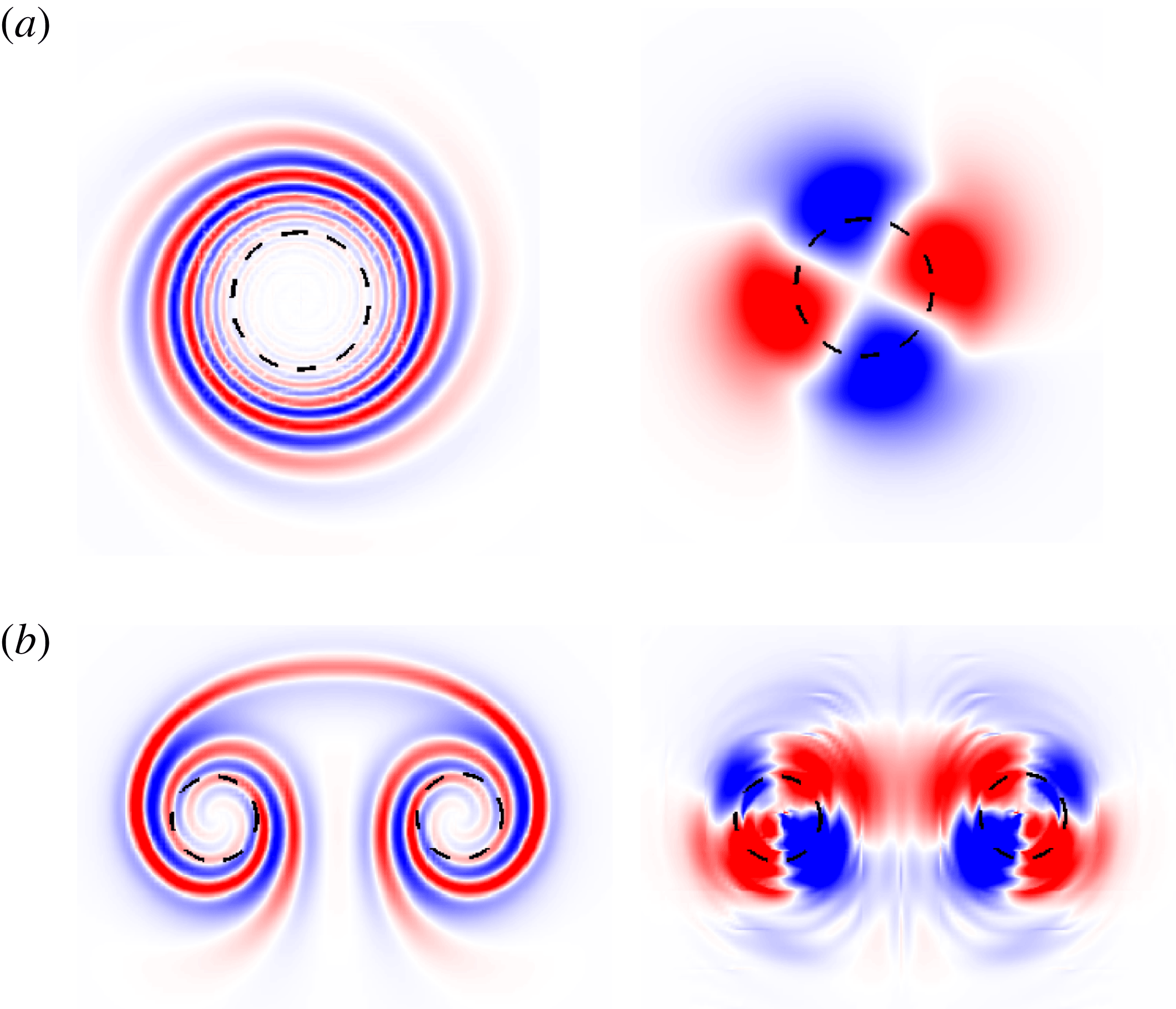
1 Introduction
From giant cyclones to small-scale structures in turbulence, vortices are present in almost all natural flows. They play a crucial role in the transport of mass, momentum and energy in flow processes. Perhaps this is why Küchemann (Reference Küchemann1965) observed that ‘vortices are the sinews and muscles of fluid motion’. As such, vortices have been extensively studied for their role in flow transition and turbulence. For a detailed examination of different types of vortical flows, the interested reader is referred to Lugt (Reference Lugt1983), Saffman (Reference Saffman1992) and Green (Reference Green1995).
The mathematical analysis of vortex systems can be traced back as early as 1880. Kelvin (Reference Kelvin1880) investigated wave motions in a column of uniform vorticity surrounded by irrotational flow (popularly referred to as the Rankine vortex model). These so-called Kelvin waves were the starting point for several later works on the dynamics of the Rankine vortex as well as other vortical flows. One such topic is the stability of vortex columns. A general perturbation to a Rankine vortex can be represented as a linear combination of the various Kelvin waves. If the perturbation is small, the nonlinear term in the flow equations can be dropped. Within the linear framework, the evolution of each wave component occurs independently from the rest. Therefore the stability of a vortex column can be determined by analysing the stability of each wave component separately. For an inviscid vortex, the waves are neutrally stable. In the presence of viscosity, the waves decay exponentially in time. For other vortex models (for example, the Lamb–Oseen vortex), additional waves can exist (Fabre, Sipp & Jacquin Reference Fabre, Sipp and Jacquin2006). Still, all waves decay exponentially under the action of viscosity. Thus, any infinitesimal perturbation to an isolated vortex will eventually decay in time.
Linear stability analysis (LSA) is useful for studying the asymptotic response of a fluid system to infinitesimal perturbations. In the long term, the least stable – or most unstable – mode is expected to dominate the flow evolution. However, many flow processes occur on a finite time scale. LSA fails to capture such transient processes that might contribute to the growth of perturbation energy (
 $E$
). The transient growth of perturbation energy is attributed to non-normality of the linearized Navier–Stokes operator (Farrell Reference Farrell1988; Trefethen et al.
Reference Trefethen, Trefethen, Reddy and Driscoll1993). As a consequence of non-normality, the eigenmodes associated with the operator are non-orthogonal. Therefore, it is possible to combine different eigenmodes and form an initial perturbation for which the rate of change of perturbation energy (
 $\text{d}E/\text{d}t$
) with time is positive, despite all the eigenmodes being linearly stable. For unstable systems, eigenmodes can be suitably combined to give a higher growth rate of perturbation energy than the most unstable eigenmode. During the transient phase (of stable/unstable flows), the perturbation may become strong enough for secondary instabilities to occur. The subsequent flow evolution will then be different from that of the linearized system. An example of such behaviour is plane Couette flow (PCF). LSA predicts that PCF is stable for all Reynolds numbers (
 $Re$
). However, experiments show that turbulence can be produced and sustained in PCF for
 $Re$
as low as
 ${\sim}300$
(Barkley Reference Barkley2016). The transient growth of perturbation energy might fill in the gap between experimental observation and results of LSA.
The inability of LSA to describe flow evolution during the transient phase motivates us to take an alternative perspective on stability of flow systems. The new approach is based on seeking a perturbation that maximizes the perturbation energy over a given horizon time (
 $T$
). We note that this approach introduces
 $T$
as a stability parameter. The perturbation satisfying the maximization criterion is referred to as the optimal perturbation and the corresponding energy gain at
 $t=T$
is the optimal gain. The shape of the optimal perturbation and the value of the optimal gain depend on
 $T$
. A recent article by Schmid & Brandt (Reference Schmid and Brandt2014) provides an overview of the various tools and techniques that have been developed to compute optimal gain and perturbations in flow systems.
The optimal perturbation for an isolated vortex has been studied mainly within the linear framework (Antkowiak & Brancher Reference Antkowiak and Brancher2004, Reference Antkowiak and Brancher2007; Pradeep & Hussain Reference Pradeep and Hussain2006; Mao & Sherwin Reference Mao and Sherwin2011, Reference Mao and Sherwin2012). Antkowiak & Brancher (Reference Antkowiak and Brancher2004) carried out optimal perturbation analysis for two-dimensional (2D) and three-dimensional (3D) perturbations with azimuthal wavenumber
 $m=1$
. They observed that the linear optimal perturbation consists of vorticity filaments in a spiral arrangement near the outer periphery of the vortex core. The energy growth mechanism was attributed to a combination of the Orr mechanism (Orr Reference Orr1907) and vortex induction. During the Orr mechanism the spiral filaments that are inclined against the base flow are uncoiled, resulting in the growth of perturbation energy. This uncoiling, in turn, was found to promote vortex induction along the vortex axis. Furthermore, they reported that the linear optimal gain for small axial wavenumbers (
 $k\rightarrow 0$
) is significantly higher than for large wavenumbers. For
 $k=0$
, the linear optimal gain was found to increase linearly with
 $T$
. Pradeep & Hussain (Reference Pradeep and Hussain2006) investigated 3D linear optimal perturbation for various
 $(m,k)$
combinations and identified the corresponding physical mechanism behind the energy growth. They reported that the axisymmetric mode (
 $m=0$
) results in the largest growth of perturbation energy in the full computational domain. The
 $m=1$
(bending) mode, on the other hand, causes the largest perturbation to the vortex core. They speculated that the bending wave might be responsible for core transition to turbulence. Antkowiak & Brancher (Reference Antkowiak and Brancher2007) observed that a perturbation consisting of a stack of azimuthal velocity streaks leads to an amplification of perturbation energy in columnar vortices. The velocity stack evolves to form vortex rings around the core of the vortex. Based on this observation, they surmised that a similar mechanism might be at play in the development of vortex rings around a columnar vortex when it is submerged in a turbulent background.
In the present work, we investigate nonlinear optimal perturbation of an isolated Lamb–Oseen vortex. The only work in this direction is by Bisanti (Reference Bisanti2013). Bisanti’s analysis was restricted to
 $m=2$
perturbations, and the value of nonlinear optimal gain obtained in the work was found to be lower than the linear optimal gain. We do not place any restriction on
 $m$
in our work. Our results show that the interaction between different azimuthal components can result in higher optimal gain than the linear optimal gain. Bisanti (Reference Bisanti2013) reported that, if the initial energy of the perturbation is large, the
 $m=2$
nonlinear optimal perturbation triggers a subcritical bifurcation to a quasi-steady rotating tripolar perturbation. The existence of quasi-steady non-axisymmetric vortex states has been established in several earlier works (e.g. Rossi, Lingevitch & Bernoff Reference Rossi, Lingevitch and Bernoff1997; Le Dizes Reference Le Dizes2000). We have studied the long-term nonlinear evolution of the linear and nonlinear optimal perturbations. Dipolar, tripolar and quadrupolar vortex states that retain their shape for several rotation periods are observed in our simulations. This suggests that optimal perturbation serves as a good initial condition to realize quasi-steady non-axisymmetric vortex states. Our work also brings out the significance of the critical layer in the evolution of non-axisymmetric vortices.
One of the major motivations for studying vortex dynamics is its application in the analysis of aircraft wakes. The vorticity sheet generated over the wings of an aircraft roll up downstream to form a pair of counter-rotating vortices. These wake vortices are quite resilient to surrounding turbulence and remain in the atmosphere for many rotation periods of the vortex. If an aircraft encounters wake vortices, there is a possibility of loss of control. Such a scenario would be catastrophic during take-off or landing, as the aircraft may not have sufficient altitude to recover. To avoid this situation, regulations have been imposed to set a minimum distance between two aircraft. This allows time for the wake vortices to decay naturally or to be convected away. Owing to the continuing increase in demand for air transport, such regulations have led to the saturation of aircraft operations in many major airports. There is an urgent need to find a solution to the saturation problem. One possibility would be to develop strategies for alleviation of wake vortices. In this regard, optimal perturbation in double-vortex systems may provide a lead. It is expected that the optimal perturbation will hasten the transition to turbulence in wake vortices, thereby rendering the wake benign for vortex encounter. Compared with the single-vortex system, the double-vortex system has been considerably less explored. The stability of a vortex pair was investigated in earlier works (e.g. Crow Reference Crow1970; Tsai & Widnall Reference Tsai and Widnall1976; Pierrehumbert Reference Pierrehumbert1980). In two dimensions, Brion, Sipp & Jacquin (Reference Brion, Sipp and Jacquin2014) showed the existence of several unstable modes for a vortex pair. Recently, Jugier (Reference Jugier2016) pursued this flow and investigated linear optimal perturbation for a pair of counter-rotating vortices. He found that a transient mechanism can lead to higher energy gain than the most unstable mode. In the present work we investigate linear and nonlinear optimal perturbations in a counter-rotating vortex pair. The vortex pair is obtained by superimposing the velocity fields for two Lamb–Oseen vortices of opposite circulation placed at a certain distance from each other, and letting the resultant flow evolve for some time. The flow evolution stage is important as the superimposed flow is not an exact solution of the Navier–Stokes equations. Such a technique has been used in earlier numerical works on double-vortex systems (Brion Reference Brion2009; Jugier Reference Jugier2016). Our results show that the mechanism of transient energy growth in a counter-rotating vortex pair is similar to that of an isolated vortex. This reinforces the relevance of studying an isolated vortex to the analysis of vortex-pair dynamics. However, unlike an isolated vortex, nonlinear transient processes do not lead to a quasi-steady dynamics for the vortex pair. Instead, the flow switches to an unstable evolution beyond a certain time. In this situation, optimal perturbation (linear/nonlinear) can be used to hasten the rate of flow destabilization.
The paper has been organized as follows. First, § 2 describes the governing equations and the optimization strategy. Next, results from optimal analysis for an isolated Lamb–Oseen vortex are presented in § 3. Results for a counter-rotating vortex pair are presented in § 4. We conclude the paper in § 5.
2 Problem formulation
2.1 Governing equations
The flow is governed by the incompressible Navier–Stokes equations
 $$\begin{eqnarray}\displaystyle \unicode[STIX]{x1D735}\boldsymbol{\cdot }\boldsymbol{u} & = & \displaystyle 0,\end{eqnarray}$$
 $$\begin{eqnarray}\displaystyle \frac{\unicode[STIX]{x2202}\boldsymbol{u}}{\unicode[STIX]{x2202}t}+(\boldsymbol{u}\boldsymbol{\cdot }\unicode[STIX]{x1D735})\boldsymbol{u} & = & \displaystyle -\unicode[STIX]{x1D735}p+\frac{1}{Re}\unicode[STIX]{x1D6FB}^{2}\boldsymbol{u},\end{eqnarray}$$
where
 $\boldsymbol{u}$
,
 $p$
and
 $Re$
are the velocity, pressure and Reynolds number, respectively. Equations (2.1) and (2.2) are accompanied by initial and boundary conditions for the flow variables. The flow (represented by
 $\boldsymbol{q}=(\boldsymbol{u},p)$
) is written as the sum of base flow (
 $\boldsymbol{Q}=(\boldsymbol{U},P)$
) and perturbation (
 $\boldsymbol{q}^{\prime }=(\boldsymbol{u}^{\prime },p^{\prime })$
),
 $$\begin{eqnarray}\displaystyle \boldsymbol{q}=\boldsymbol{Q}+\boldsymbol{q}^{\prime }. & & \displaystyle\end{eqnarray}$$
The decomposition (2.3) is generally useful when the base state evolves on a time scale that is much slower than the evolution of the perturbation. More often than not, the steady solution of (2.1) and (2.2) is selected as the base flow. Substituting (2.3) into (2.1) and (2.2) and subtracting from it the equations for the base state, we get the equations governing the evolution of the perturbation:
 $$\begin{eqnarray}\displaystyle \unicode[STIX]{x1D735}\boldsymbol{\cdot }\boldsymbol{u}^{\prime } & = & \displaystyle 0,\end{eqnarray}$$
 $$\begin{eqnarray}\displaystyle \frac{\unicode[STIX]{x2202}\boldsymbol{u}^{\prime }}{\unicode[STIX]{x2202}t}+(\boldsymbol{U}\boldsymbol{\cdot }\unicode[STIX]{x1D735})\boldsymbol{u}^{\prime }+(\boldsymbol{u}^{\prime }\boldsymbol{\cdot }\unicode[STIX]{x1D735})\boldsymbol{U}+(\boldsymbol{u}^{\prime }\boldsymbol{\cdot }\unicode[STIX]{x1D735})\boldsymbol{u}^{\prime } & = & \displaystyle -\unicode[STIX]{x1D735}p^{\prime }+\frac{1}{Re}\unicode[STIX]{x1D6FB}^{2}\boldsymbol{u}^{\prime }.\end{eqnarray}$$
Equations (2.4) and (2.5) are accompanied by initial conditions for the perturbation (
 $\boldsymbol{q}_{t=0}^{\prime }$
) and homogeneous boundary conditions. In the linear framework, the nonlinear term
 $(\boldsymbol{u}^{\prime }\boldsymbol{\cdot }\unicode[STIX]{x1D735})\boldsymbol{u}^{\prime }$
is dropped from (2.5).
2.2 Optimization
We seek an initial perturbation (
 $\boldsymbol{q}_{0}^{\prime }$
) that maximizes the gain of perturbation kinetic energy over a given horizon time
 $T$
. The kinetic energy associated with the perturbation at any time instant is taken as
 $$\begin{eqnarray}\displaystyle E(t)=\int _{\unicode[STIX]{x1D6FA}}\boldsymbol{u}^{\prime }(t)\boldsymbol{\cdot }\boldsymbol{u}^{\prime }(t)\,\text{d}\unicode[STIX]{x1D6FA}, & & \displaystyle\end{eqnarray}$$
where
 $\unicode[STIX]{x1D6FA}$
is the computational domain. The energy gain with respect to the initial perturbation is
 $$\begin{eqnarray}\displaystyle G(\boldsymbol{q}_{0}^{\prime },t)=E(t)/E(0), & & \displaystyle\end{eqnarray}$$
where
 $E(0)$
is the energy of the perturbation at
 $t=0$
. Therefore, the optimal perturbation maximizes the value of
 $G$
at
 $T$
. We use the method of Lagrange multipliers to solve the optimization problem. The Lagrangian functional,
 ${\mathcal{L}}$
, is defined as
 $$\begin{eqnarray}\displaystyle {\mathcal{L}}(\boldsymbol{q}^{\prime },\boldsymbol{q}^{+},\boldsymbol{q}_{0}^{\prime },\boldsymbol{q}_{0}^{+},\unicode[STIX]{x1D706})=G(\boldsymbol{q}_{0}^{\prime };T)-\langle \boldsymbol{q}^{+},\boldsymbol{F}(\boldsymbol{q}^{\prime })\rangle -\unicode[STIX]{x1D706}(E_{0}-E(0)), & & \displaystyle\end{eqnarray}$$
where
 $\boldsymbol{F}(\boldsymbol{q}^{\prime })=0$
represents the equation system (2.4) and (2.5) (or the linearized version of it for linear optimization),
 $\boldsymbol{q}^{+}$
and
 $\unicode[STIX]{x1D706}$
are the Lagrange multipliers and
 $\langle \cdot ,\cdot \rangle$
denotes the inner product of two vectors,
 $$\begin{eqnarray}\displaystyle \langle \boldsymbol{a},\boldsymbol{b}\rangle =\int _{T}\int _{\unicode[STIX]{x1D6FA}}\boldsymbol{a}\boldsymbol{\cdot }\boldsymbol{b}\,\text{d}\unicode[STIX]{x1D6FA}\,\text{d}t. & & \displaystyle\end{eqnarray}$$
Here,
 $\boldsymbol{F}$
is usually referred to as the Navier–Stokes operator. The boundary conditions accompanying equations (2.4) and (2.5) are implicit in the definition of
 ${\mathcal{L}}$
. The parameter
 $E_{0}$
constrains the kinetic energy of the perturbation at
 $t=0$
to a fixed value (equal to
 $E_{0}$
) via the last term on the right-hand side of (2.8). The constraint is set using a geometric update technique described later in this section. The optimization procedure, therefore, yields optimal perturbation/gain corresponding to a given value of
 $E_{0}$
. Within the linear framework, the optimal gain is independent of the initial energy of the perturbation. Nonlinear optimal gain/perturbation, on the other hand, depends on the value of
 $E_{0}$
.
For optimality, the gradient of
 ${\mathcal{L}}$
with respect to all the variables should be zero. Setting to zero the gradient of
 ${\mathcal{L}}$
with respect to
(ii)
 $\boldsymbol{q}^{\prime }$
, gives the adjoint equations (2.10)$$\begin{eqnarray}\displaystyle \unicode[STIX]{x1D735}\boldsymbol{\cdot }\boldsymbol{u}^{+}=0, & & \displaystyle\end{eqnarray}$$
(2.11)$$\begin{eqnarray}\displaystyle & & \displaystyle \frac{\unicode[STIX]{x2202}\boldsymbol{u}^{+}}{\unicode[STIX]{x2202}t}+(\boldsymbol{U}\boldsymbol{\cdot }\unicode[STIX]{x1D735})\boldsymbol{u}^{+}+(\boldsymbol{u}^{\prime }\boldsymbol{\cdot }\unicode[STIX]{x1D735})\boldsymbol{u}^{+}\nonumber\\ \displaystyle & & \displaystyle \qquad =\boldsymbol{u}^{+}\boldsymbol{\cdot }(\unicode[STIX]{x1D735}\boldsymbol{U})^{\text{T}}+\boldsymbol{u}^{+}\boldsymbol{\cdot }(\unicode[STIX]{x1D735}\boldsymbol{u}^{\prime })^{\text{T}}-\unicode[STIX]{x1D735}p^{+}-\frac{1}{Re}\unicode[STIX]{x1D6FB}^{2}\boldsymbol{u}^{+};\end{eqnarray}$$
(iii)
$\boldsymbol{q}_{0}^{+}$
, gives the compatibility equation (2.12)$$\begin{eqnarray}\displaystyle \boldsymbol{u}^{+}(T)=2\frac{\boldsymbol{u}^{\prime }(T)}{E_{0}}; & & \displaystyle\end{eqnarray}$$
(iv)
$\boldsymbol{q}_{0}^{\prime }$
, gives the optimality equation (2.13)$$\begin{eqnarray}\displaystyle \unicode[STIX]{x1D735}_{\boldsymbol{q}_{0}^{\prime }}{\mathcal{L}}=\boldsymbol{u}^{+}(0)-2\frac{E_{T}}{E_{0}^{2}}\boldsymbol{u}^{\prime }(0). & & \displaystyle\end{eqnarray}$$


For a detailed derivation of (2.10)–(2.13) the interested reader is referred to Farrell (Reference Farrell1988), Corbett & Bottaro (Reference Corbett and Bottaro2000), Zuccher, Bottaro & Luchini (Reference Zuccher, Bottaro and Luchini2006), Cherubini et al. (Reference Cherubini, De Palma, Robinet and Bottaro2011), Cherubini & De Palma (Reference Cherubini and De Palma2013), Schmid & Brandt (Reference Schmid and Brandt2014) and Kerswell (Reference Kerswell2018).
An iterative procedure is employed to arrive at the optimal initial condition. Each iteration loop consists of the following four steps:
(1) equations (2.4) and (2.5) (also referred to as direct equations) are marched forwards in time from
$t=0$
to
$T$
;(2) equation (2.12) is used to compute the adjoint field at
$T$
;(3) equations (2.10) and (2.10) are solved backwards in time from
$t=T$
to
$t=0$
;(4) equation (2.13) along with the geometric update technique proposed by Douglas, Amari & Kung (Reference Douglas, Amari and Kung2000) are used to set the next guess for
$\boldsymbol{q}_{0}^{\prime }$
.


The geometric update technique sets the initial energy of the perturbation. First, the component of
 $\unicode[STIX]{x1D735}_{\boldsymbol{q}_{0}^{\prime }}{\mathcal{L}}$
that is normal to
 $\boldsymbol{q}_{0}^{\prime }$
is scaled as per the initial energy constraint,
 $$\begin{eqnarray}\displaystyle \boldsymbol{N}^{\,j}=E(0)^{1/2}\frac{\unicode[STIX]{x1D735}_{\boldsymbol{q}_{0}^{\prime }}{\mathcal{L}}_{\bot }}{\Vert \unicode[STIX]{x1D6FB}_{\boldsymbol{q}_{0}^{\prime }}{\mathcal{L}}_{\bot }\Vert }, & & \displaystyle\end{eqnarray}$$
where
 $j$
is the iteration number and
 $\bot$
denotes the normal component. The initial perturbation for step 1 of the next iteration is then given by
 $$\begin{eqnarray}\displaystyle \boldsymbol{q}_{0}^{\prime \,j+1}=\boldsymbol{q}_{0}^{\prime \,j}\cos (\unicode[STIX]{x1D6FC})+\boldsymbol{N}^{\,j}\sin (\unicode[STIX]{x1D6FC}). & & \displaystyle\end{eqnarray}$$
In (2.15),
 $\unicode[STIX]{x1D6FC}$
is the step length and its starting value is unity. A simplified line search is implemented to choose the right value of
 $\unicode[STIX]{x1D6FC}$
. If at the end of step 1 the energy gain has a higher value than the previous iteration, then
 $\unicode[STIX]{x1D6FC}$
is not changed. If the gain is lower than the previous gain,
 $\unicode[STIX]{x1D6FC}$
is reduced successively by a factor of 2 until the energy gain has a higher value compared to the last iteration. For the first iteration loop, the initial perturbation for step 1 is random white noise. In linear optimization the terms
 $(\boldsymbol{u}^{\prime }\boldsymbol{\cdot }\unicode[STIX]{x1D735})\boldsymbol{u}^{+}$
and
 $\boldsymbol{u}^{+}\boldsymbol{\cdot }(\unicode[STIX]{x1D735}\boldsymbol{u}^{\prime })^{\text{T}}$
are not present in (2.10).
The computations have been carried out using Nek5000 (Fischer, Lottes & Kerkemeier Reference Fischer, Lottes and Kerkemeier2008), which is an open-source spectral element solver for incompressible and weakly compressible flows. For the single-vortex system, a circular computational domain is used. For the double-vortex system, computations are carried out in a rectangular domain. The computational domain is divided into a large number of spectral elements. Each spectral element is further discretized using Gauss–Lobatto–Legendre (GLL) points. Near the vortex core region, the spatial resolution of the mesh is kept high in order to capture the flow gradients accurately. The resolution decreases towards the boundary of the computational domain. Convergence studies have been carried out to establish the adequacy of the extent of the computational domain and mesh resolution. The effect of the size of the computational domain for an isolated vortex is discussed in § 3.2.2.
2.3 Linear stability analysis of Lamb–Oseen vortex
The flow state is written in normal-mode representation,
 $$\begin{eqnarray}\displaystyle \boldsymbol{q}^{\prime }(r,\unicode[STIX]{x1D703},t)=\hat{\boldsymbol{q}}(r)\text{e}^{\text{i}m\unicode[STIX]{x1D703}}\text{e}^{\unicode[STIX]{x1D706}t}, & & \displaystyle\end{eqnarray}$$
where
 $m$
is the azimuthal wavenumber, and
 $\hat{\boldsymbol{q}}$
and
 $\unicode[STIX]{x1D706}$
are complex quantities. Substituting (2.16) in the linearized version of (2.4) and (2.5), we get a generalized eigenvalue problem:
 $$\begin{eqnarray}\displaystyle \unicode[STIX]{x1D63C}\hat{\boldsymbol{q}}=\unicode[STIX]{x1D706}\unicode[STIX]{x1D63D}\hat{\boldsymbol{q}}. & & \displaystyle\end{eqnarray}$$
The real and imaginary parts of
 $\unicode[STIX]{x1D706}$
correspond to the growth rate and frequency of the eigenmode, respectively. In the discrete version of the problem,
 $\unicode[STIX]{x1D63C}$
and
 $\unicode[STIX]{x1D63D}$
are non-symmetric matrices. A shift-inverse transformation is used to compute the eigenmodes and eigenvalues.
3 Isolated vortex
3.1 Base flow
The base flow for carrying out the optimal analysis is a Lamb–Oseen vortex. Its velocity distribution in the cylindrical coordinate system is given by
 $$\begin{eqnarray}\displaystyle u_{r}=0,\quad u_{\unicode[STIX]{x1D703}}=\frac{\unicode[STIX]{x1D6E4}}{2\unicode[STIX]{x03C0}r}(1-\text{e}^{-r^{2}/a^{2}}), & & \displaystyle\end{eqnarray}$$
where
 $u_{r}$
and
 $u_{\unicode[STIX]{x1D703}}$
are the radial and azimuthal components of velocity,
 $\unicode[STIX]{x1D6E4}$
is the circulation associated with the Lamb–Oseen vortex,
 $a$
is the vortex dispersion radius and
 $r$
is the distance from the origin. The vortex strength (
 $\unicode[STIX]{x1D6E4}$
) is related to vorticity (
 $\unicode[STIX]{x1D714}$
) by
 $$\begin{eqnarray}\displaystyle \unicode[STIX]{x1D6E4}=\int _{\unicode[STIX]{x1D734}}\unicode[STIX]{x1D714}\,\text{d}\unicode[STIX]{x1D734}. & & \displaystyle\end{eqnarray}$$
In (3.2), the integration is carried out over the entire computational domain. The vortex dispersion radius (
 $a$
) is given by
 $$\begin{eqnarray}\displaystyle a=\sqrt{\frac{\displaystyle \int _{\unicode[STIX]{x1D734}}r^{2}\unicode[STIX]{x1D714}\,\text{d}\unicode[STIX]{x1D734}}{\unicode[STIX]{x1D6E4}}}. & & \displaystyle\end{eqnarray}$$
The Lamb–Oseen vortex is assumed to be frozen in time. The length and velocity scales have been rendered non-dimensional using
 $a$
and
 $\unicode[STIX]{x1D6E4}/2\unicode[STIX]{x03C0}a$
, respectively. The Reynolds number (
 $Re=\unicode[STIX]{x1D6E4}/2\unicode[STIX]{x03C0}\unicode[STIX]{x1D708}$
) for all simulations is
 $Re=5000$
. Bernoff & Lingevitch (Reference Bernoff and Lingevitch1994) analysed the relaxation of a perturbed Gaussian vortex and found that the perturbations evolve on an
 $Re^{1/3}$
time scale. For
 $Re=5000$
, the time scale for evolution of the perturbation is several orders lower than that for viscous dissipation (
 $\unicode[STIX]{x1D70F}_{\unicode[STIX]{x1D708}}=2\unicode[STIX]{x03C0}a^{2}/\unicode[STIX]{x1D708}$
). It is, therefore, reasonable to assume that the base flow is steady during perturbation evolution. This is confirmed in appendix A where optimization results obtained for
 $T=4.8$
using an evolving base flow are found to be nearly the same as those obtained using the frozen base-flow approach. For very large horizon times the frozen base-flow approach is inadequate and serves as an approximation. Compared to an evolving base flow, the frozen base-flow approach has significant advantages in terms of computational memory and time.
3.2 Linear analysis
3.2.1 Optimal gain and perturbation
Optimal perturbation for an isolated vortex has been studied mostly in three dimensions and almost exclusively within the linear framework (Antkowiak & Brancher Reference Antkowiak and Brancher2004, Reference Antkowiak and Brancher2007; Pradeep & Hussain Reference Pradeep and Hussain2006). Antkowiak & Brancher (Reference Antkowiak and Brancher2004) investigated linear optimal perturbation (LO-P) for azimuthal wavenumber
 $m=1$
. In the present study, we extend the 2D optimization work of Antkowiak & Brancher (Reference Antkowiak and Brancher2004) by considering additional wavenumbers.
The general perturbed state of a Lamb–Oseen vortex is amenable to Fourier decomposition in the azimuthal direction:
 $$\begin{eqnarray}\displaystyle \boldsymbol{q}^{\prime }(r,\unicode[STIX]{x1D703},t)=\mathop{\sum }_{m\in \mathbb{Z}}\boldsymbol{q}_{m}(r,t)\text{e}^{\text{i}m\unicode[STIX]{x1D703}}+\text{c.c.} & & \displaystyle\end{eqnarray}$$
Here
 $(r,\unicode[STIX]{x1D703})$
represents a spatial location with respect to the centre of the cylindrical coordinate system,
 $m$
is the azimuthal wavenumber, that takes non-negative integer (
 $\mathbb{Z}$
) values, and c.c. denotes the complex conjugate. In the linear framework, different azimuthal components evolve independently from one another. Therefore, we carry out linear optimization for different wavenumbers
 $m$
separately. Linear optimal gain (LO-G) for a given horizon time
 $T$
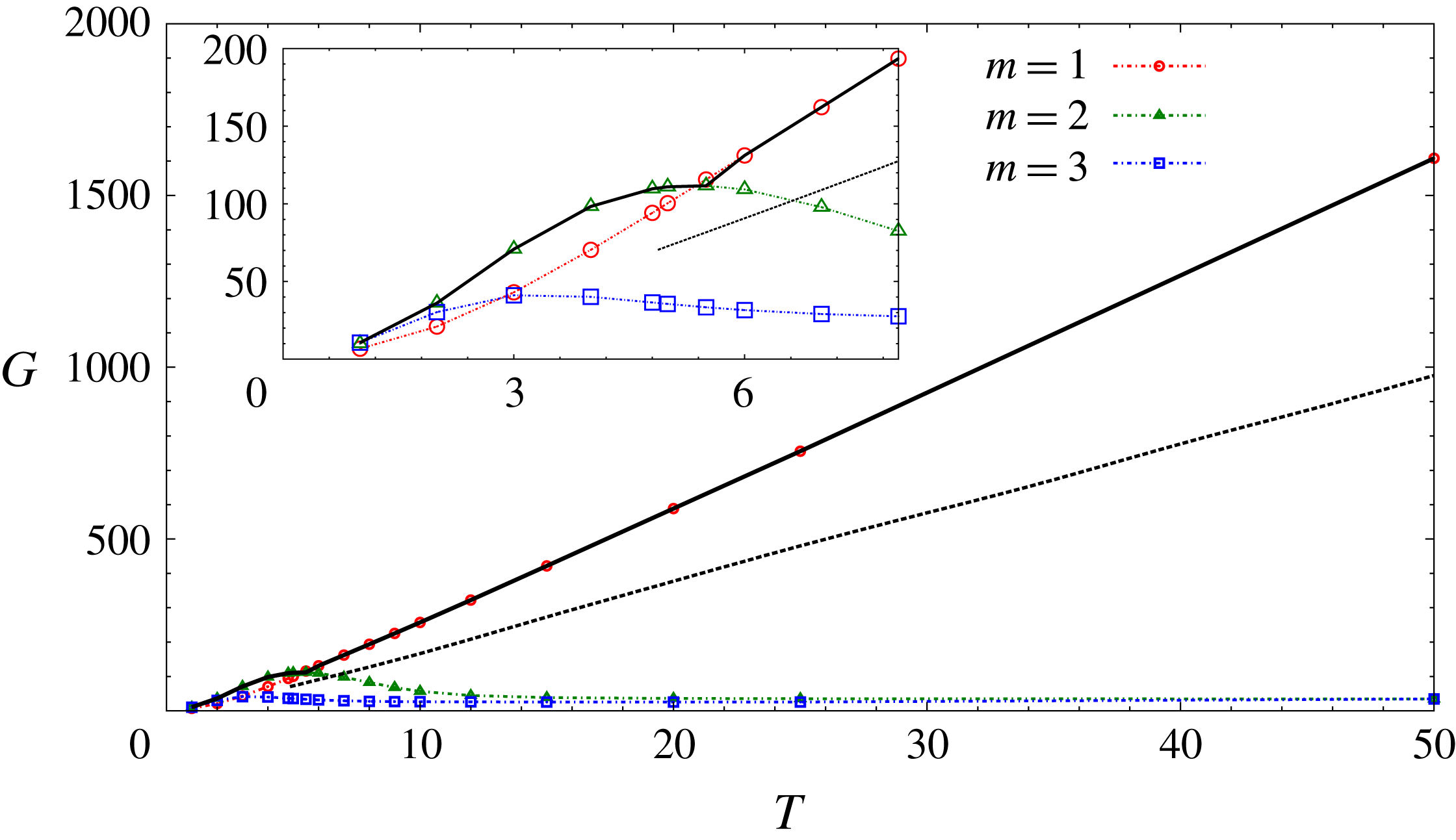
is the largest gain of all azimuthal wavenumbers. Figure 1 shows the variation of largest gain with
 $T$
for various
 $m$
. The horizon time has been rendered non-dimensional by the rotation period of the base flow (
 $\unicode[STIX]{x1D70F}=4\unicode[STIX]{x03C0}^{2}a^{2}/\unicode[STIX]{x1D6E4}$
). The LO-G curve, shown as a thick solid line in figure 1, is the envelope of the different
 $m$
gain curves. It is observed that LO-G increases with
 $T$
up to the largest horizon time that has been studied. For
 $T<5.5$
, the optimal perturbation has azimuthal wavenumber
 $m>1$
. For
 $T\geqslant 5.5$
, LO-P corresponds to
 $m=1$
. A kink is observed in the LO-G curve at
 $T=5.5$
that marks the shift of LO-P from
 $m=2$
to 1 (see the inset of figure 1). For
 $T\geqslant 5.5$
the optimal gain increases linearly with
 $T$
. This is consistent with the
 $Re=1000$
result of Antkowiak & Brancher (Reference Antkowiak and Brancher2004). The gain curve reported by them is shown by a dashed line in figure 1. The slope of the LO-G curve for
 $Re=5000$
is higher than that for
 $Re=1000$
. Accordingly, as
 $T$
increases, the difference between LO-G for the two Reynolds numbers grows.
Results for
 $Re=5000$
isolated vortex: variation of the largest energy gain with the horizon time for
 $m=1$
, 2 and 3. The linear optimal gain curve is the envelope of the gain curves for different
 $m$
and is shown by a thick solid line. Inset is a magnified view of the part of the gain curve where the linear optimal perturbation switches from
 $m>1$
to
 $m=1$
. The variation of the 2D linear optimal gain for
 $Re=1000$
and
 $m=1$
reported by Antkowiak & Brancher (Reference Antkowiak and Brancher2004) is shown by a dashed line.

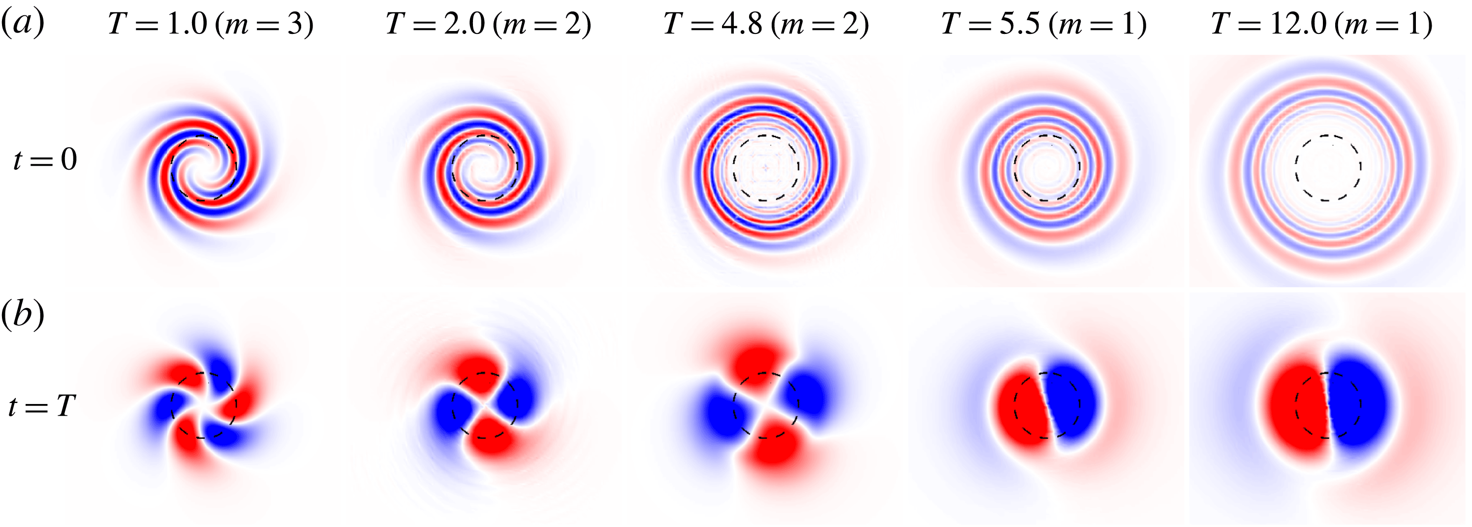
Results for
 $Re=5000$
isolated vortex: (a) vorticity field of the linear optimal perturbation for varying horizon time; (b) the corresponding vorticity field at the horizon time
 $t=T$
.
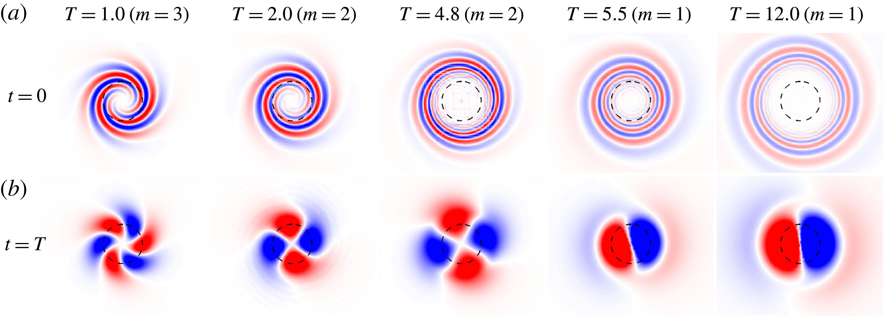
The vorticity field associated with LO-P for different horizon times is shown in figure 2(a). In figure 2(b), the corresponding evolved vorticity field at
 $t=T$
is shown. LO-P consists of vorticity filaments in spiral arrangement. Energy growth for such flow structures is attributed to the Orr mechanism (Orr Reference Orr1907). The Orr mechanism is typical of plane shear flows. Its relevance in rotational flows has been demonstrated by Antkowiak & Brancher (Reference Antkowiak and Brancher2004) and Pradeep & Hussain (Reference Pradeep and Hussain2006). As
 $T$
increases, the vortex filaments move away from the vortex centre. During the flow evolution, the vorticity filaments uncoil. For large
 $T$
, a dipolar perturbation appears in and around the core region of the vortex. This can be observed in the last column of figure 2. The effect of the dipolar structure is to shift the vortex core from its unperturbed location. For lower horizon times (
 $T<5.5$
), the optimal perturbation leads to a quadrupolar (
 $m=2$
) or a hexapolar (
 $m=3$
) structure, which does not induce any shift in the position of the vortex core.
3.2.2 Long-term linear evolution of the linear optimal perturbation
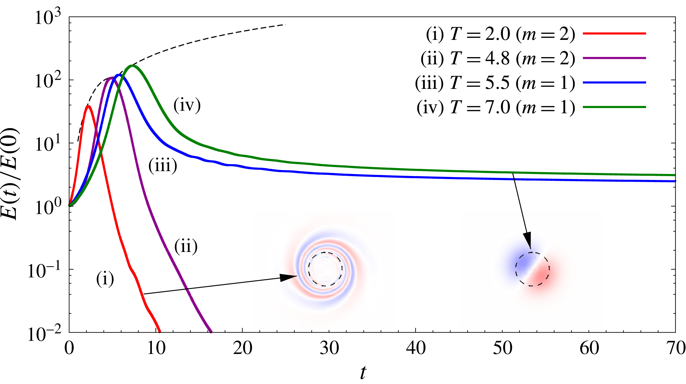
Results for
 $Re=5000$
isolated vortex: evolution of the energy gain with time for computations initiated with the linear optimal perturbation corresponding to different horizon times. The azimuthal wavenumber of linear optimal perturbation is written inside parentheses in the legend. The evolution of perturbation is governed by the linearized version of equation system (2.4) and (2.5). The variation of the linear optimal gain with
 $T$
is shown using a dashed line. The long-term perturbation vorticity field for the computations initiated with the
 $T=2.0$
and 7.0 linear optimal perturbations are shown as insets. The time instants from which the two fields are taken are marked by arrows.

Direct time integration of the linearized version of (2.4), (2.5) is carried out using LO-P for various
 $T$
as the initial condition. The time evolution of the energy gain is shown in figure 3. In each case, the gain reaches a peak value and then decreases rapidly. The peak gain corresponding to each
 $T$
is nearly the same as LO-G for the same
 $T$
. For
 $T<5.5$
, the gain continues to decrease rapidly even at large times. The long-term perturbation field consists of vorticity filaments similar to those of the initial perturbation but in an opposite spiral arrangement (inset of figure 3; cf. figure 2). For
 $T\geqslant 5.5$
the rapid decay of perturbation energy seems to arrest after some time. Subsequently the energy decays very slowly and the perturbation has a dipolar structure (see inset of figure 3).
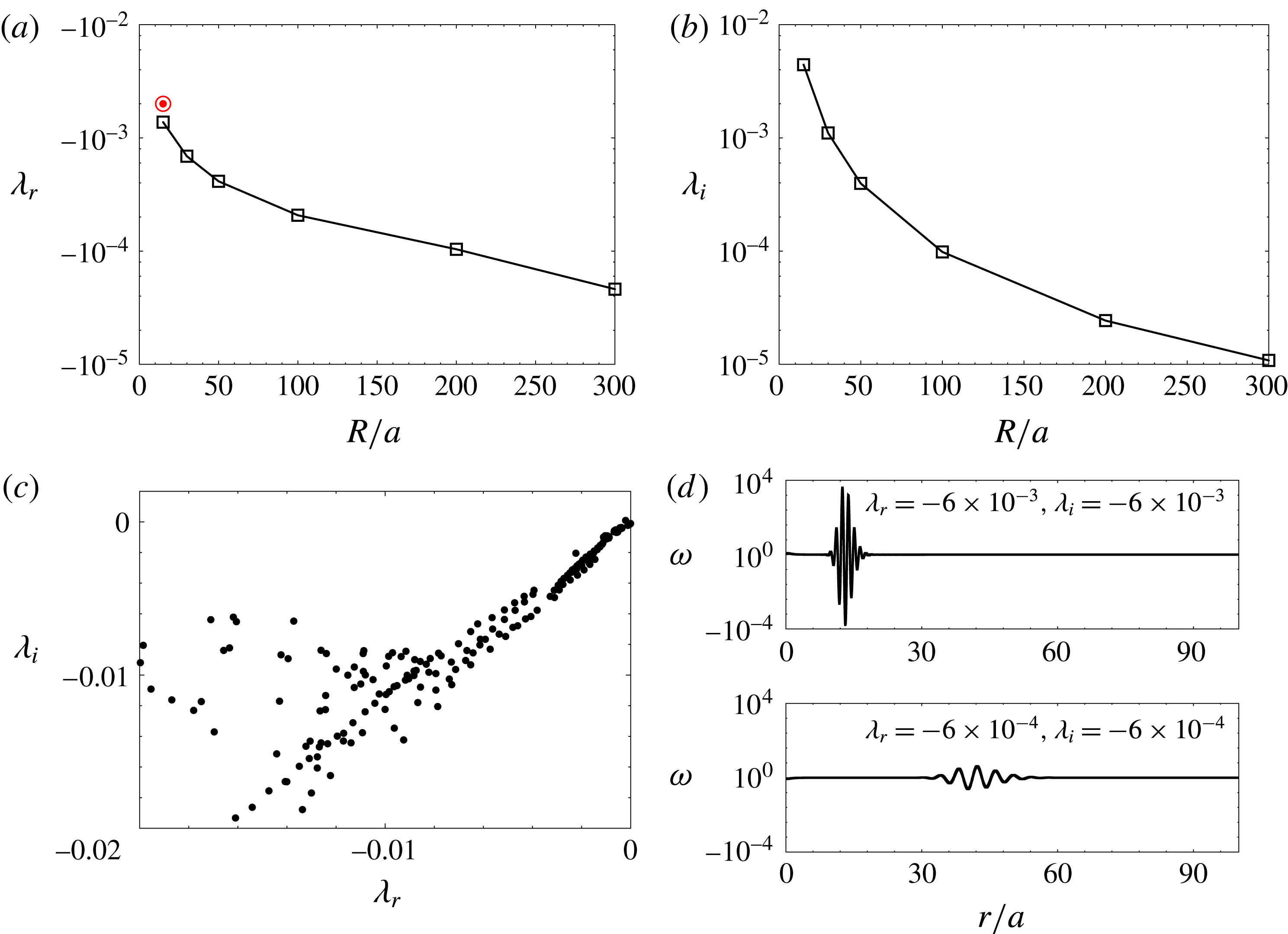
LSA results for
 $Re=5000$
of an isolated Lamb–Oseen vortex: variation of the non-dimensional (a) growth rate and (b) frequency of the displacement mode with the size of the computational domain. The results have been rendered non-dimensional with respect to the rotation time of the vortex
 $\unicode[STIX]{x1D70F}$
. The growth rate of the perturbation calculated using the energy decay rate at large time for
 $T=7.0$
in figure 3 is shown by a bull’s eye symbol. (c) Part of the continuous spectrum for
 $m=1$
. (d) Vorticity distributions for eigenmodes from the continuous spectrum corresponding to two eigenvalues. Here
 $r$
denotes the radial distance from the origin of the cylindrical coordinate system.

LO-P for a given horizon time can be written as a linear combination of the eigenmodes of the linearized Navier–Stokes operator (Pradeep & Hussain Reference Pradeep and Hussain2006). Owing to the non-orthogonality of the eigenmodes, transient growth of perturbation energy is possible in vortex systems (Antkowiak & Brancher Reference Antkowiak and Brancher2004; Pradeep & Hussain Reference Pradeep and Hussain2006). However, in the long term, the most unstable or the least stable mode is expected to dominate the flow evolution. Fabre et al. (Reference Fabre, Sipp and Jacquin2006, hereafter FSJ 2006) carried out LSA of a Lamb–Oseen vortex and found that all the eigenmodes, other than the 2D displacement mode (
 $m=1$
), have negative growth rate. The 2D displacement mode is neutrally stable and its effect on the base flow is to shift the location of the vortex centre. It is observed that the long-term perturbation field for
 $T\geqslant 5.5$
in figure 3 is very similar to the 2D displacement mode. This implies that the 2D displacement mode contributes to the LO-P for
 $T\geqslant 5.5$
. As the 2D displacement mode has zero growth rate, the perturbation energy at large time is expected not to vary with time. We, however, observe that the perturbation energy decays slowly at large time. The reason for this is the finiteness of the computational domain used for the present work. To elucidate this, we present the variation of the growth rate (
 $\unicode[STIX]{x1D706}_{r}$
) and the frequency (
 $\unicode[STIX]{x1D706}_{i}$
) of the 2D displacement mode obtained via LSA (§ 2.3) with the radius of the computational domain (
 $R$
) in figures 4(a) and 4(b), respectively. It can be observed that both
 $\unicode[STIX]{x1D706}_{r}$
and
 $\unicode[STIX]{x1D706}_{i}$
are close to, but not equal to, zero. Both quantities seem to approach zero as
 $R\rightarrow \infty$
. Owing to the negative growth rate of the 2D displacement mode in the finite domain, the perturbation decays long term for
 $T\geqslant 5.5$
. This is confirmed by noting that the decay rate derived from the energy evolution curve for
 $T\geqslant 5.5$
at large time (shown by the bull’s eye symbol in figure 4
a) is close to the growth rate of the 2D displacement mode obtained via LSA. The difference between the two values is because of the presence of other modes, albeit with lower magnitude than the 2D displacement mode. If the linearized simulations are carried on further, the difference is expected to become smaller.
Effect of the size of the computational domain on the value of optimal gain for
 $T=4.8$
and 7.0 (
 $R$
is the radius of the computational domain). The nonlinear gains are for
 $E(0)=0.01$
.
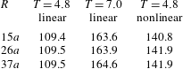
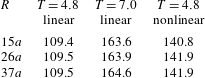
A question that arises in view of the sensitivity of LSA results to the extent of the computational domain is: Does the size of the domain affect the value of the LO-G? Our computations show that, beyond a certain radial extent, LO-G is unaffected. Table 1 lists the values of LO-G for
 $T=4.8$
and 7.0 for different values of domain radius
 $R$
. The suitable size of the computational domain for optimal analysis depends on the horizon time
 $T$
. This is because the vortex filaments of the LO-P move away from the vortex centre as
 $T$
increases. In the present case
 $R=15a$
appears to be adequate to carry out linear optimization at least up to
 $T=7$
.
Figure 1 shows that LO-G increases monotonically with
 $T$
. Therefore, a Lamb–Oseen vortex can support transient growth up to very large horizon times, despite being linearly stable. The reason is understood to be the existence of a continuous spectrum for the Lamb–Oseen vortex. Mao & Sherwin (Reference Mao and Sherwin2011, Reference Mao and Sherwin2012) found that, in addition to the discrete spectrum, two continuous spectra exist for the Batchelor vortex. The tangential and radial velocity distributions of a Batchelor vortex are similar to those of a Lamb–Oseen vortex. However, unlike a Lamb–Oseen vortex, which is a 2D model, a Batchelor vortex is characterized by a Gaussian distribution of axial velocity. As for the Batchelor vortex, a continuous spectrum exists for a Lamb–Oseen vortex as well. Figure 4(c) shows a part of the continuous spectrum of a Lamb–Oseen vortex for
 $m=1$
. The computations have been carried out in a domain of radial length
 $R=100a$
. It is observed that the modes from the continuous spectrum can have a very low decay rate. The lower the decay rate, the further the mode is located from the vortex core (figure 4
d). The discrete modes are generally located near the vortex centre (FSJ 2006). We recall that, with increasing
 $T$
, LO-P moves away from the vortex centre. Therefore, LO-P at large
 $T$
is constituted of modes from the continuous spectrum that have a low decay rate. Consequently, the continuous spectrum and the 2D displacement mode combine to exhibit transient growth of perturbation energy up to very large values of horizon time.
We end this section on linear analysis with a short note on the applicability of finite-domain simulations. In practical scenarios, an isolated vortex does not exist. In most situations, a vortex belongs to part of a multi-vortex system, for example, trailing vortices in the wake of an aircraft. The effect of surrounding vortices in such situations can be emulated by using appropriate boundary conditions, albeit in a finite domain. We would like to point out that in practice it is impossible to carry out infinite-domain computations.
3.3 Nonlinear analysis
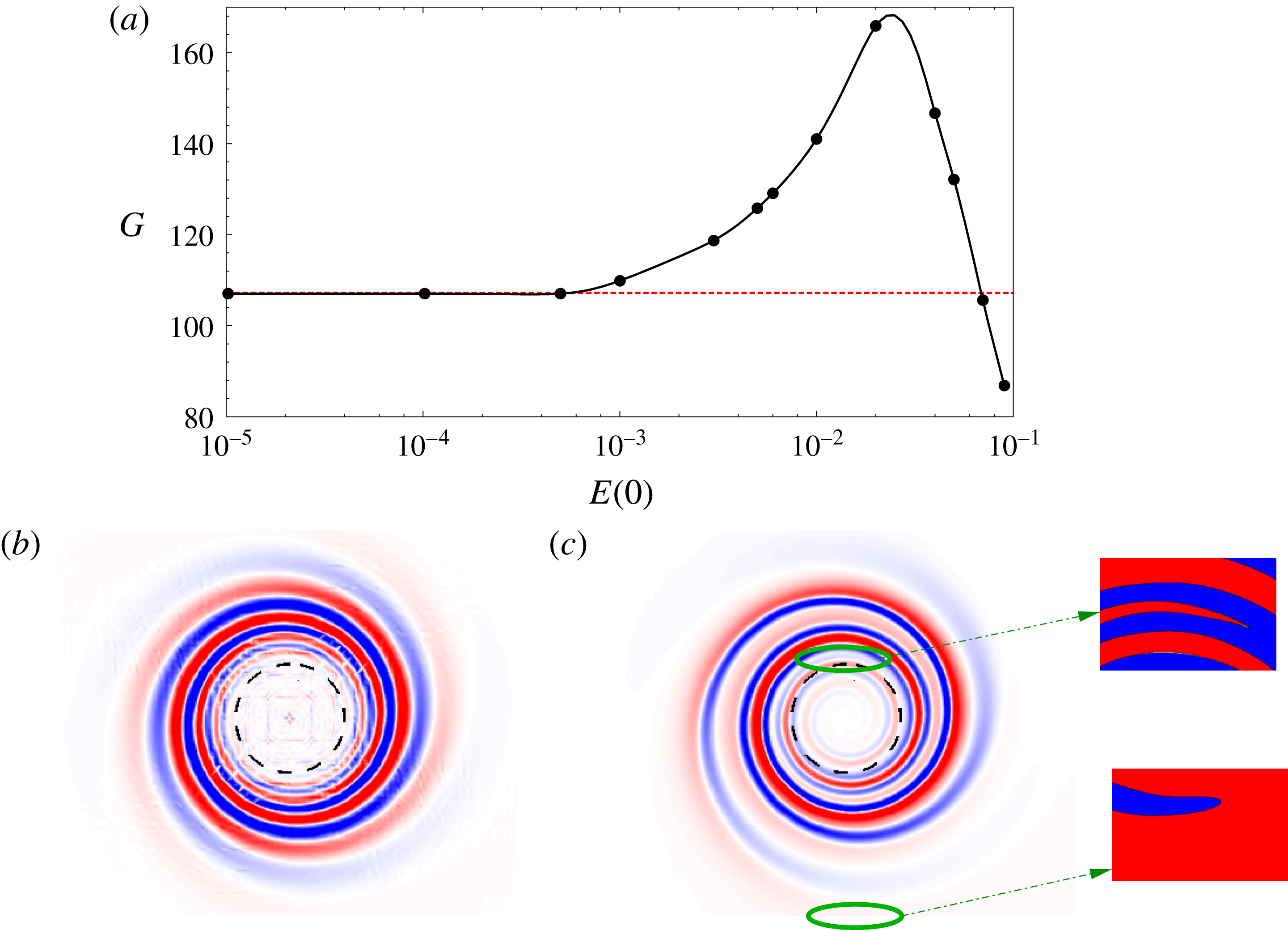
Results for
 $Re=5000$
isolated vortex: (a) variation of the nonlinear optimal gain for
 $T=4.8$
with initial energy of the perturbation. The azimuthal velocity field associated with nonlinear optimal perturbation (at
 $t=0$
) for
 $E(0)=10^{-4}$
and
 $E(0)=3\times 10^{-3}$
is shown in (b) and (c), respectively. A magnified view of the two spiral dislocations in the nonlinear optimal perturbation is provided. A synthetic two-colour scheme has been used in the magnified view to display the dislocations clearly. In (a) the value of the linear optimal gain is indicated by a dashed line.

Recent works on nonlinear optimization of flows (like boundary layer flow, PCF) have shown that, for the same horizon time, nonlinear optimal perturbation (NLO-P) can result in higher gain than LO-P (Cherubini et al.
Reference Cherubini, De Palma, Robinet and Bottaro2011; Cherubini & De Palma Reference Cherubini and De Palma2013; Kerswell Reference Kerswell2018). We extend nonlinear optimization to the Lamb–Oseen vortex. Nonlinear optimization is carried out by retaining the nonlinear terms in the direct-adjoint iterative process (§ 2.2). The adjoint equations require the input of the direct perturbation field. Hence, the time history of the direct flow is saved at each iteration of the optimization process. This increases the computational cost significantly when compared with linear optimization. Unlike for LO-G, nonlinear optimal gain (NLO-G) depends on the initial energy of the perturbation (
 $E(0)$
). Therefore, the nonlinear framework presents a richer parameter space than the linear framework. For each horizon time, computations are carried out for varying values of
 $E(0)$
. The general variation of NLO-G with
 $E(0)$
is found to be similar for different horizon times
 $T$
. We have selected
 $T=4.8$
to present a detailed analysis. Unless stated otherwise, the results for nonlinear optimization of the isolated vortex are for
 $T=4.8$
.
3.3.1 Optimal gain
Figure 5(a) provides the variation of NLO-G with
 $E(0)$
for
 $T=4.8$
. The corresponding LO-G is shown using a dashed line in the same panel. For low values of the initial energy (
 $E(0)\leqslant 5\times 10^{-4}$
), NLO-G is nearly the same as LO-G. Beyond
 $E(0)=5\times 10^{-4}$
, NLO-G departs from the linear value. At first, NLO-G increases with
 $E(0)$
and reaches a peak value for
 $E(0)=0.03$
. The NLO-G value for
 $E(0)=0.03$
is
 ${\sim}50\,\%$
higher than LO-G. With further increase in
 $E(0)$
, NLO-G decreases monotonically;
 $G$
becomes lower than LO-G for
 $E(0)\geqslant 0.07$
. Therefore, there exists a range of
 $E(0)$
for which NLO-P yields higher gain than the LO-P.
Table 1 demonstrates the effect of the size of the computational domain on the value of NLO-G. Similarly to LO-G, the NLO-G for
 $T\leqslant 7.0$
is unaffected by expansion of the domain beyond
 $15a$
.
Cherubini & De Palma (Reference Cherubini and De Palma2013) investigated NLO-P for PCF and reported a similar variation of NLO-G with
 $E(0)$
as in figure 5(a). Unlike in the present work they considered 3D perturbations in their analysis. We note that the base state for both flows is 2D and linearly stable. In both flows, there exists a threshold value of
 $E(0)$
below which NLO-G remains nearly the same as LO-G; above the threshold value, NLO-G shows significant departure from LO-G. However, unlike PCF, where NLO-G remains higher than LO-G for
 $E(0)$
greater than the threshold, NLO-G for a 2D Lamb–Oseen vortex becomes lower than the LO-G for large values of
 $E(0)$
. The explanation may be that in PCF, for large values of
 $E(0)$
, the flow field at the horizon time becomes turbulent. With the restriction of 2D perturbation for Lamb–Oseen vortex, there is no possibility of flow transition even with large
 $E(0)$
, and any initial perturbation must eventually decay as suggested by the result of LSA.
3.3.2 Optimal perturbation
Figures 5(b) and 5(c) give the vorticity fields associated with NLO-P for
 $E(0)=10^{-4}$
and
 $3\times 10^{-3}$
, respectively. We recall that the LO-P for
 $T=4.8$
has azimuthal wavenumber of
 $m=2$
(figure 1). The shape of NLO-P for
 $E(0)=10^{-4}$
is very similar to that of the
 $m=2$
linear optimal. Thus, for low
 $E(0)$
, both NLO-G as well as the shape of NLO-P are similar to those obtained via linear analysis. This is so because the contribution of the nonlinear terms to the evolution of the perturbation becomes smaller as
 $E(0)$
tends to zero. Beyond the threshold energy (
 $E(0)>5\times 10^{-4}$
), two major differences are observed with respect to the LO-P. First, the vorticity filaments far from the vortex core appear less diffused. Second, two spiral dislocations are observed. A spiral dislocation is identified by the merger of two vorticity filaments of the same sign. In figure 5(c), the locations of the two spiral dislocations is shown by solid ellipses. The dislocations are situated at distances of
 ${\sim}1.1a$
and
 ${\sim}3.6a$
from the vortex centre. A magnified view of the two dislocations using a synthetic two-colour scale is provided in figure 5(c). In the first dislocation (
 $r\sim 1.1a$
), two negative vorticity filaments, which are separated by a positive vorticity filament, merge. In the second dislocation (
 $r\sim 3.6a$
), two positive vorticity filaments merge. The general shape of NLO-P for
 $E(0)>5\times 10^{-4}$
is similar.
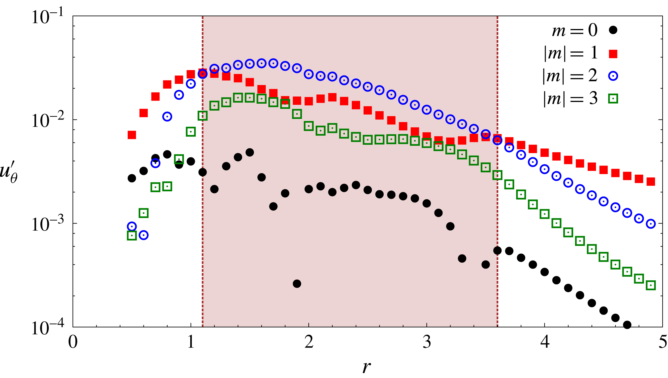
Results for
 $Re=5000$
isolated vortex: Fourier decomposition of the azimuthal component of the
 $T=4.8$
,
 $E(0)=3\times 10^{-3}$
nonlinear optimal perturbation (
 $t=0$
) velocity field at various radial locations. Here
 $m$
is the azimuthal wavenumber. The shaded part corresponds to the radial segment between the two spiral dislocations in the nonlinear optimal perturbation shown in figure 5(c).

Figure 6 shows the relative contribution of different azimuthal wavenumbers to the
 $E(0)=3\times 10^{-3}$
NLO-P as a function of distance from the vortex centre. The contributions of
 $|m|\geqslant 4$
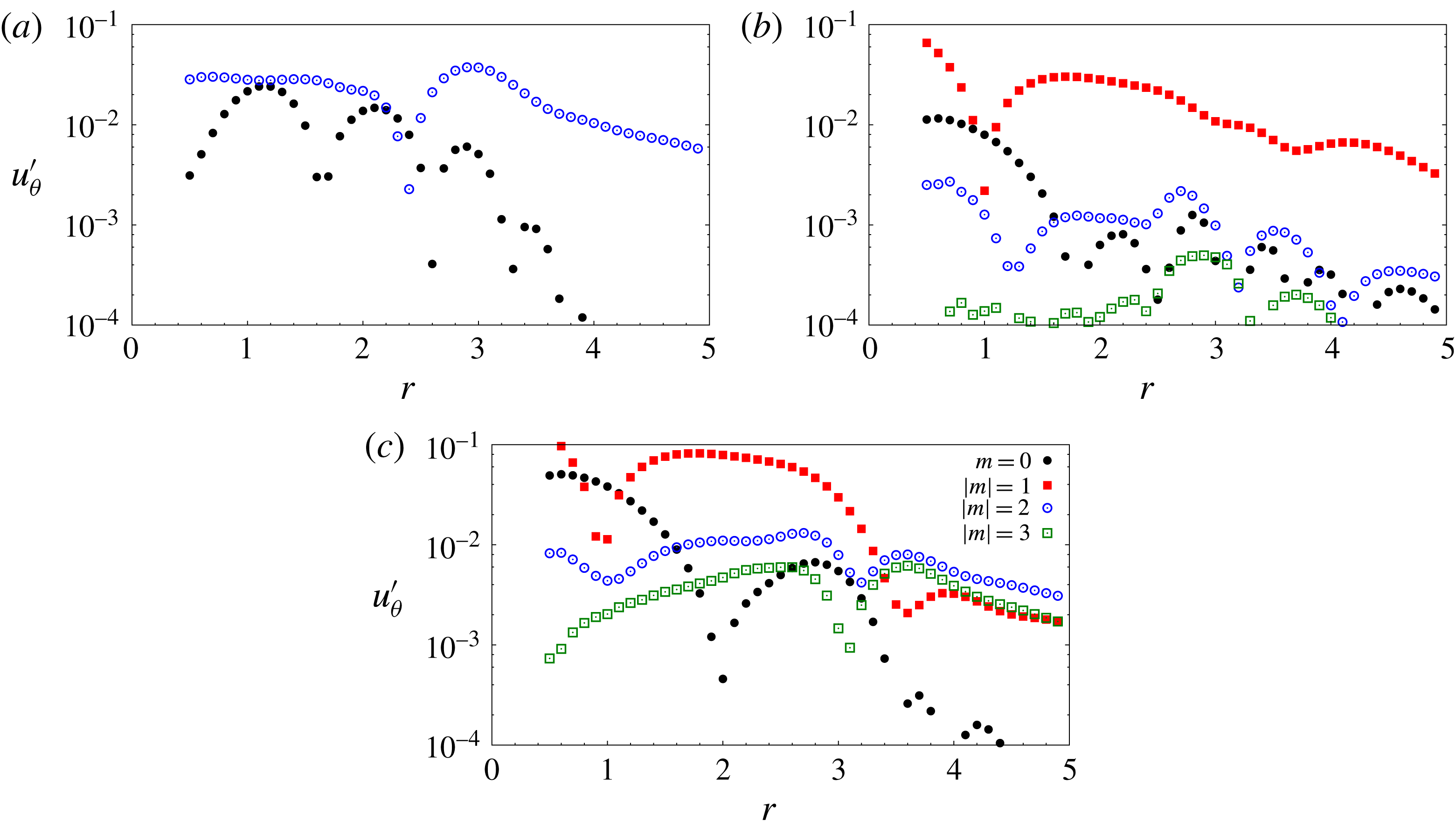
are relatively small and hence are not included in figure 6. The data have been generated by using Fourier decomposition of the azimuthal component of the perturbation velocity for several radial locations. Unlike LO-P, NLO-P has contributions from different azimuthal wavenumbers. At any given radial location, the azimuthal mean of the velocity is non-zero, as indicated by the presence of
 $m=0$
component. Among the non-zero wavenumbers, the most significant contribution to NLO-P is from
 $m=1$
and
 $2$
. The shaded region in figure 6 corresponds to the radial location between the two spiral dislocations in NLO-P (figure 5
c). It is observed that in the shaded part
 $m=2$
is the most dominant component, whereas outside the shaded part the most dominant wavenumber is
 $m=1$
. It appears that spiral dislocation is the consequence of the switch in the dominant wavenumber within the NLO-P.
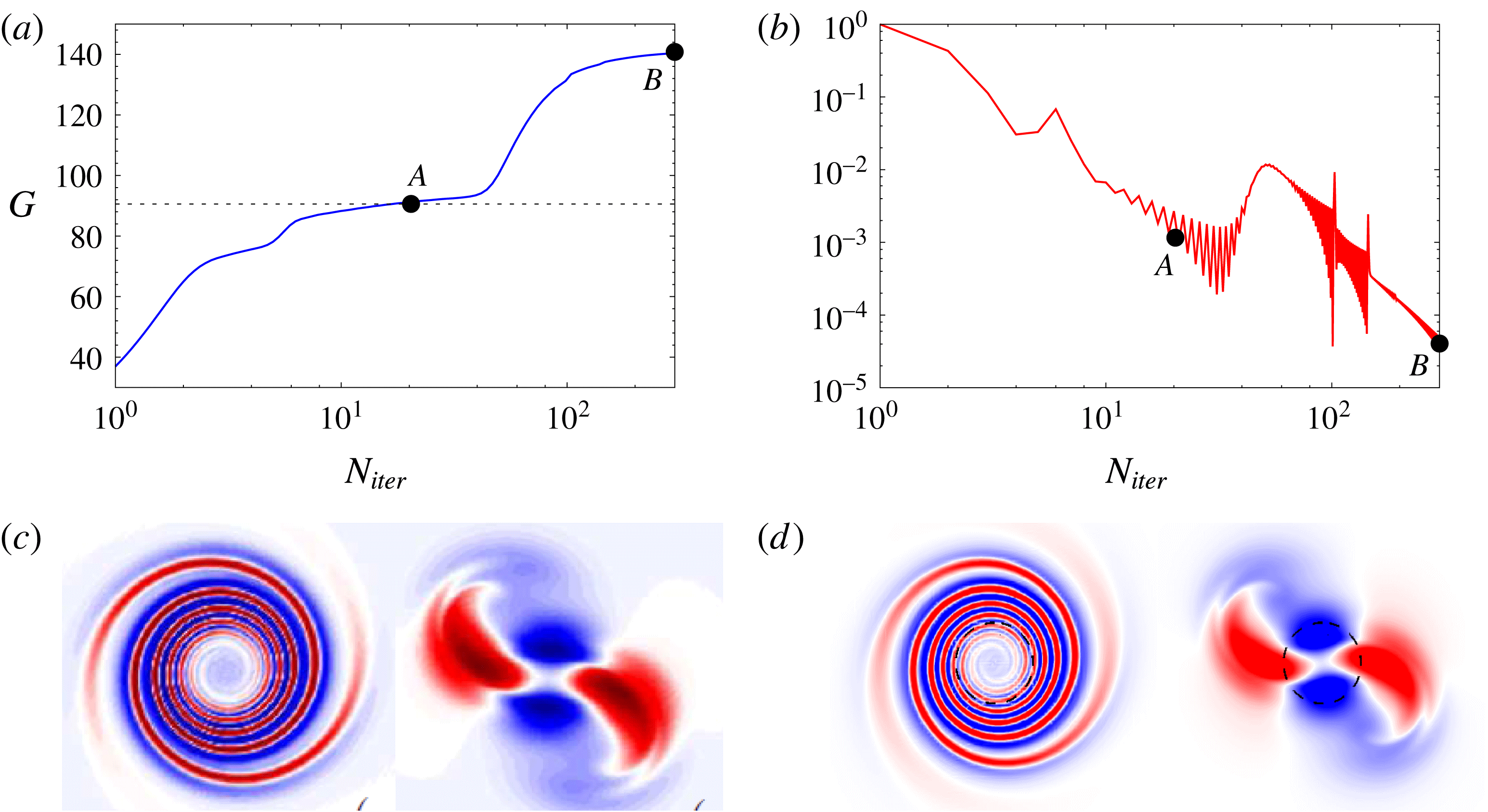
Results for
 $Re=5000$
isolated vortex: variation of (a) the nonlinear optimal gain and (b) the increment in gain with iteration number during the optimization process for
 $T=4.8$
and
 $E(0)=0.01$
. The suboptimal and optimal states are labelled
 $A$
and
 $B$
, respectively. The optimal gain reported by Bisanti (Reference Bisanti2013) is indicated by a dashed line in (a). (c) Vorticity field for the
 $m=2$
optimal perturbation and its evolved state at
 $t=T$
as reported by Bisanti (Reference Bisanti2013). (d) Vorticity field for suboptimal perturbation and its evolved state at
 $t=T$
as obtained in the present work.

Recently, Bisanti (Reference Bisanti2013) investigated NLO-P for a 2D Lamb–Oseen vortex. The work was restricted to
 $m=2$
perturbations. For
 $T=4.8$
and
 $E(0)=0.01$
Bisanti (Reference Bisanti2013) found the value of NLO-G to be lower than LO-G. Our computations show that for the same parameters NLO-G is higher than LO-G (figure 5
a). Figure 7(a) shows the variation of energy gain with iteration number during the optimization process for
 $T=4.8$
and
 $E(0)=0.01$
. It is observed that, close to the value of the optimal gain reported by Bisanti (Reference Bisanti2013), the variation of gain seems to plateau (point
 $A$
); the increment in the value of optimal gain with each iteration (
 $J$
) is
 $O\sim 10^{-3}$
and it decreases near point
 $A$
(see figure 7
b). We refer to point
 $A$
as a suboptimal state. Figure 7(c) shows the vorticity field corresponding to the optimal perturbation and its evolved state at
 $t=T$
as reported by Bisanti (Reference Bisanti2013). Figure 7(d) gives the same field for the suboptimal state obtained in the present work. The fields are very similar; therefore the suboptimal state corresponds to the
 $m=2$
optimal state reported by Bisanti (Reference Bisanti2013). If the iterations are continued further,
 $J$
starts to increase again. The value of gain increases with
 $N_{iter}$
and a converged state (point
 $B$
) is reached with higher energy gain. Beyond point
 $B$
, the energy gain does not change significantly with
 $N_{iter}$
up to
 $N_{iter}\sim 500$
, which is when we terminate the nonlinear optimization process. The value of
 $J$
in the converged state is
 $O\sim 10^{-5}$
. As shown in figure 6, NLO-P for
 $T=4.8$
and
 $E(0)=0.01$
has, in addition to
 $m=2$
, significant contributions from other azimuthal wavenumbers. The difference between the optimal gain reported by Bisanti (Reference Bisanti2013) and NLO-G of the present work is therefore attributed to nonlinear interactions between different azimuthal components. We would like to mention here that, in nonlinear optimization with the direct-adjoint technique, it is not possible to completely ascertain if point
 $B$
is the global optimum. We carried out
 $T=4.8$
,
 $E(0)=0.01$
nonlinear optimization with different initial guesses, for example, random perturbation, linear/nonlinear optimal perturbation for different
 $T$
. In each case the converged solution corresponds to point
 $B$
. It is, therefore, likely that point
 $B$
is the global optimum, and that there is no jump in energy gain beyond point
 $B$
in figure 7(a).
3.3.3 Effect of the horizon time
Results for
 $Re=5000$
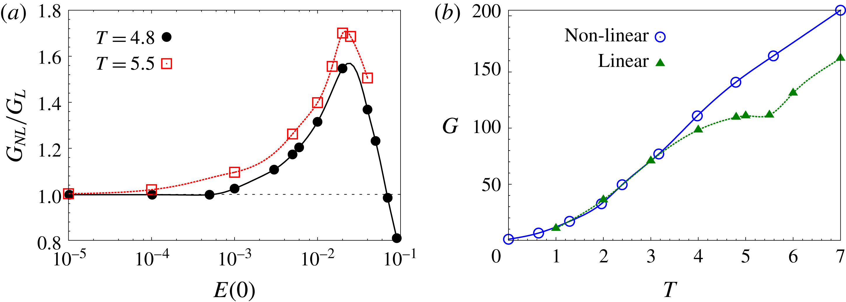
isolated vortex: variation of (a) the ratio between the nonlinear optimal gain and the LO-G with initial energy of the perturbation for
 $T=4.8$
and 5.5, and (b) linear and
 $E(0)=0.01$
nonlinear optimal gain with horizon time.

Figure 8(a) displays the effect of
 $T$
on NLO-G. For a given initial energy of the perturbation, NLO-G increases with
 $T$
. The peak optimal gain for different
 $T$
occurs for nearly the same value of
 $E(0)$
. It is observed that the threshold energy below which the NLO-G and the LO-G are nearly the same decreases with increasing
 $T$
. The threshold energies for
 $T=4.8$
and
 $5.5$
are
 $10^{-3}$
and
 $10^{-4}$
, respectively. Figure 8(b) shows the variation of NLO-G for
 $E(0)=10^{-2}$
with horizon time. For
 $T\leqslant 3.0$
, the linear and nonlinear optimal gains are nearly the same. This implies that the threshold energy for
 $T\leqslant 3.0$
is higher than
 $10^{-2}$
. For
 $T>3.0$
, the threshold energy is lower than
 $10^{-2}$
and the linear and nonlinear optimal gains are different. The difference between LO-G and NLO-G increases with
 $T$
up to
 $T=7.0$
. The threshold energy decreases with increasing
 $T$
.
3.3.4 Long-term nonlinear evolution of linear and nonlinear optimal perturbation: appearance of a quasi-steady non-axisymmetric vortex
Rossi et al. (Reference Rossi, Lingevitch and Bernoff1997) carried out numerical simulations to investigate the evolution of non-axisymmetric perturbations to a 2D Lamb–Oseen vortex. They observed that, for weak non-axisymmetric perturbation, the vortex relaxes towards an axisymmetric state. If, however, the perturbation is strong enough, a quasi-steady non-axisymmetric vortex state can be reached. A quasi-steady vortex, as defined by Rossi et al. (Reference Rossi, Lingevitch and Bernoff1997), is one that maintains approximately the same relative distribution of vorticity over several rotation periods of the vortex and diffuses on a slow time scale. The results presented in the previous sections show that linear and nonlinear optimal perturbations can result in a large energy gain at the horizon time. Furthermore, the evolved perturbation field at the horizon time is non-axisymmetric. Therefore, it is plausible that, as the perturbation relaxes from its high energy state, the vortex might exhibit quasi-steady non-axisymmetric behaviour. To explore this, we carry out direct time integration of the equations (2.4) and (2.5) governing the nonlinear evolution of the perturbations. The computations are initiated with optimal perturbations, linear and nonlinear, for various
 $T$
.
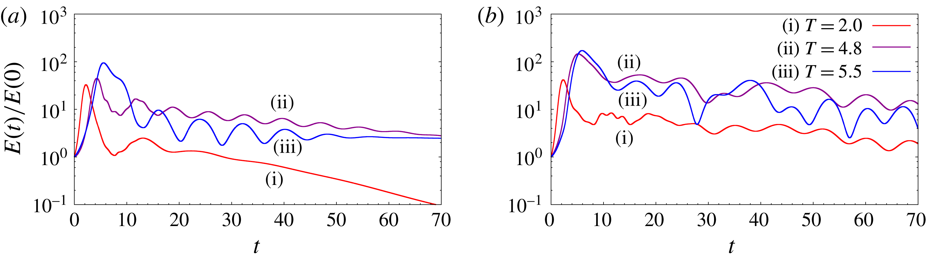
Results for
 $Re=5000$
isolated vortex: evolution of energy gain with time for computations initiated with (a) linear optimal perturbation and (b)
 $E(0)=0.01$
nonlinear optimal perturbation, for different horizon times. The evolution of perturbation is governed by equation system (2.4) and (2.5).

First, we present results from computations initiated with LO-P. The initial perturbation energy for all of the computations is
 $E(0)=10^{-2}$
. Figure 9(a) shows the temporal evolution of the perturbation energy for
 $T=2.0$
, 4.8 and 5.5 LO-P. The perturbation energy (
 $E$
) has been normalized by
 $E(0)$
. Initially,
 $E$
grows in time and its evolution is very similar to that obtained via linear simulation (figure 3). It attains a peak value near the horizon time. The peak value of
 $E$
obtained from the nonlinear computation is lower than that of the linear computation. The differences between the peak linear and nonlinear perturbation energies for
 $T=2.0$
, 4.8 and 5.5 are 14 %, 58 % and 21 %, respectively. After reaching the peak,
 $E$
decreases for some time and then exhibits fluctuations. For
 $T=2$
, the fluctuations decay rapidly and thereafter
 $E$
decreases monotonically with time. However, for
 $T=4.8$
and 5.5, the energy fluctuations persist for a long time (more than 40 rotation periods of the vortex) and are quasi-periodic. Two time scales can be identified for
 $T=4.8$
and 5.5. The slow time scale corresponds to the decrease in the mean value of perturbation energy per cycle of energy fluctuation. The fast time scale corresponds to the time period of energy fluctuation. Figures 10(a) and 11(a) show the variation of energy on the fast time scale for
 $T=4.8$
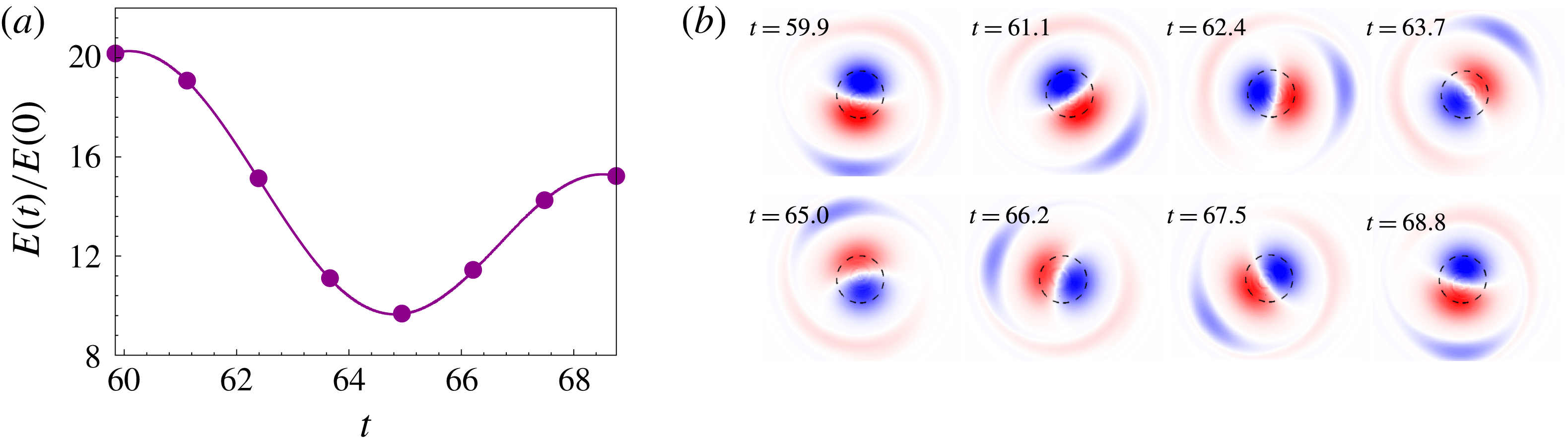
and 5.5, respectively. The fast time scale is attributed to energy exchange between the base flow and perturbation. During one half of the cycle, the perturbation draws energy from the base flow; and in the other half, the perturbation returns energy to the base flow. The periodic fluctuation of perturbation energy is associated with the quasi-steady non-axisymmetric vortex state (discussed in the next paragraph). Since viscous effects in the quasi-steady state take place on the slow time scale (Rossi et al.
Reference Rossi, Lingevitch and Bernoff1997), we attribute the decrease in mean energy per cycle of energy fluctuation to viscosity.
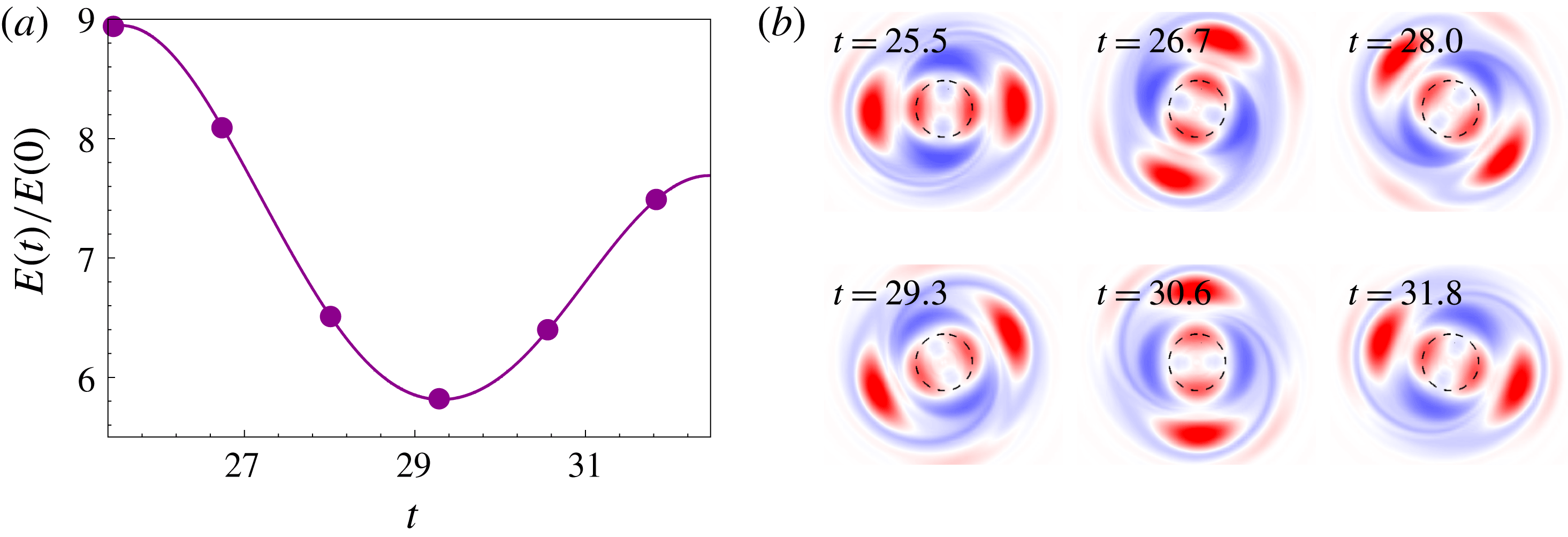
Results for
 $Re=5000$
isolated vortex: (a) variation of the energy gain during one rotation period of the quasi-steady non-axisymmetric state for computations initiated with the
 $T=4.8$
LO-P; (b) the perturbation vorticity field at various time instants marked by solid circles in the gain curve.

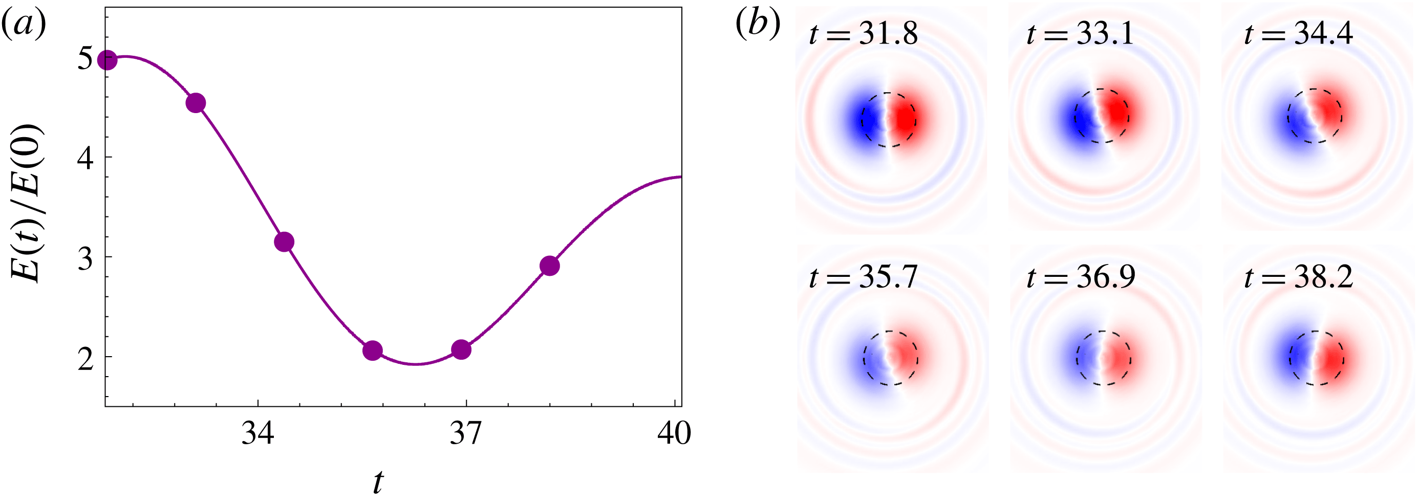
Results for
 $Re=5000$
isolated vortex: (a) variation of the energy gain during one rotation period of the quasi-steady non-axisymmetric state for computations initiated with the
 $T=5.5$
LO-P; (b) the perturbation vorticity field at various time instants marked by solid circles in the gain curve.

Results for
 $Re=5000$
isolated vortex: Fourier decomposition of the azimuthal component of perturbation velocity in the azimuthal direction at a time instant in the quasi-steady non-axisymmetric state for computations initiated with (a) the
 $T=4.8$
LO-P, (b) the
 $T=5.5$
LO-P, and (c) the
 $T=4.8$
,
 $E(0)=0.01$
NLO-P. The time instants are
 $t=25.5$
, 31.8 and 59.9, respectively.

Results for
 $Re=5000$
isolated vortex: variation of the contribution of different azimuthal components of perturbation velocity in the azimuthal direction with time, for nonlinear simulation initiated with
 $T=4.8$
LO-P and
 $E(0)=0.01$
. The key is the same as in figure 12.

Results for
 $Re=5000$
isolated vortex: (a,c,e) displacement of the vortex centre with time for computations initiated with the LO-P for (a,b)
 $T=2.0$
, (c,d)
 $T=4.8$
and (e,f
)
 $T=5.5$
; (b,d,f) corresponding trajectory of the vortex centre in the
 $X{-}Y$
plane.

Figure 10(b) shows the perturbation vorticity field at different time instants over a cycle of energy fluctuation for
 $T=4.8$
. The perturbation has non-axisymmetric structure; at least six regions of concentrated vorticity can be identified in figure 10(b). A Fourier decomposition of the perturbation field in the azimuthal direction shows that only the
 $m=0$
(axisymmetric) and
 $m=2$
components are significant (figure 12
a). We recall that in the linear framework the evolutions of different azimuthal components occur independently from one another. Hence, during linearized evolution of
 $T=4.8$
LO-P, the perturbation flow at any time instant is
 $m=2$
. Nonlinear effects, on the other hand, may allow transfer of energy between different azimuthal components. To monitor the transfer of energy from the
 $m=2$
component to other components during nonlinear evolution of
 $T=4.8$
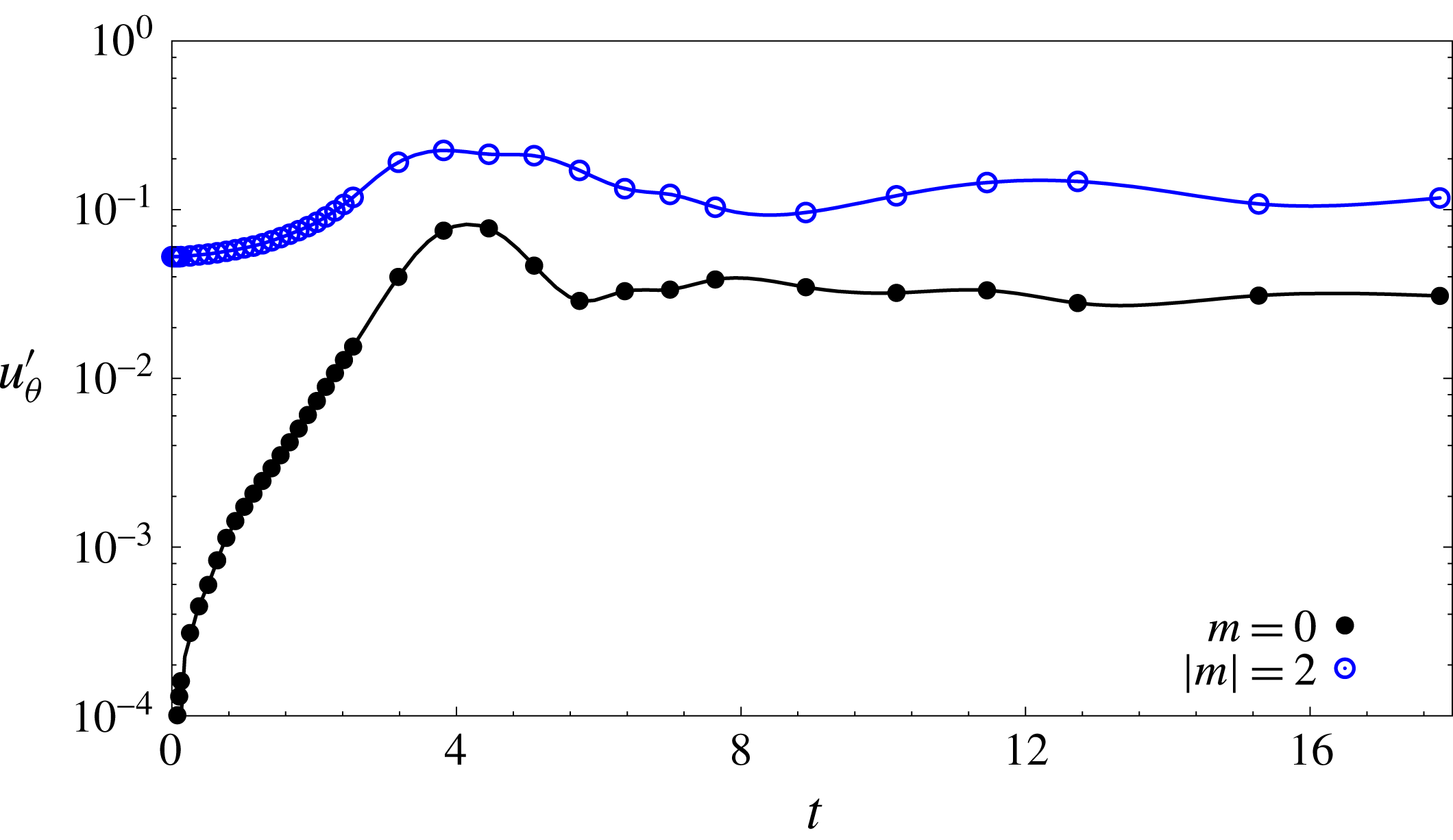
LO-P, we plot the time evolution of the relative contribution of different azimuthal components to the perturbation flow. The plots are shown in figure 13. It is observed that, as the flow evolves with time, the axisymmetric component in the flow becomes comparable to the
 $m=2$
component beyond
 $t\sim 2$
. The contribution of other azimuthal components remains relatively small during the flow evolution (and are not shown in figure 13). The perturbation field (figure 10
b) rotates in time and the relative orientation of the vorticity patches remains the same during rotation. The rotation period of the perturbation is equal to the time period of energy fluctuation. As the mean energy decreases on a slow time scale, the non-axisymmetric perturbation remains in the flow for several rotation periods. Such a perturbation state, based on the definition used by Rossi et al. (Reference Rossi, Lingevitch and Bernoff1997), corresponds to a quasi-steady non-axisymmetric perturbation. Figure 11(b) shows the perturbation vorticity field during a cycle of energy fluctuation for the
 $T=5.5$
case: a quasi-steady non-axisymmetric state exists for this case as well. The perturbation field is dominated by the
 $m=1$
component (figure 12
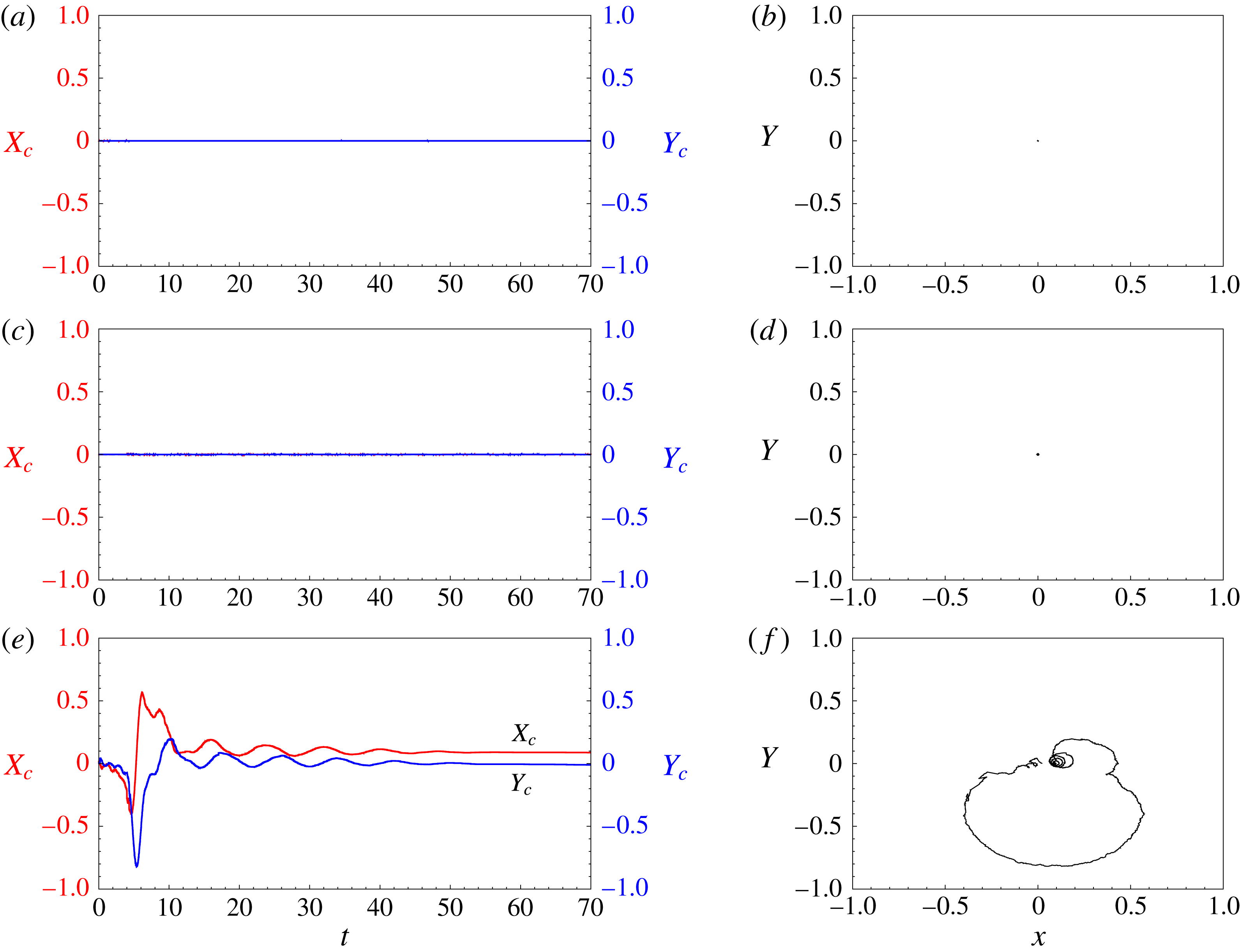
b). Near the vortex centre the perturbation has dipolar structure. The dipole does not rotate completely about the vortex; instead it exhibits small rotational oscillations about the vortex centre. The oscillation manifests in the movement of the vortex core. This can be observed in figure 14(e,f), which shows the time history of the location of the vortex centre. The location of the vortex centre is the barycentre of vorticity for the total flow, that is, base flow added with perturbation. Figure 14(a,c,e) shows the displacement of the vortex centre along the
 $X$
- and
 $Y$
-axes, and the right column shows the trajectory of the vortex centre. The
 $X$
- and
 $Y$
-axes are oriented along the horizontal and vertical directions with the origin at the centre of the unperturbed vortex. Unlike in the
 $T=5.5$
case, the vortex centre does not move significantly for the
 $T=2.0$
and 4.8 cases (figure 14
a–d).
Results for
 $Re=5000$
isolated vortex: (a) displacement of the vortex centre with time for computations initiated with the
 $T=4.8$
,
 $E(0)=0.01$
nonlinear optimal perturbation; (b) trajectory of the vortex centre in the vortex plane.

Results for
 $Re=5000$
isolated vortex: (a) variation of the energy gain during one rotation period of the quasi-steady non-axisymmetric state for computations initiated with the
 $T=4.8$
,
 $E(0)=0.01$
nonlinear optimal perturbation; (b) the perturbation vorticity fields at the time instants marked by solid circles in the gain curve.

Next we present results from computations initiated with the
 $E(0)=0.01$
NLO-P. Figure 9(b) gives the evolution of the perturbation energy for
 $T=2.0$
, 4.8 and 5.5. Similarly to the LO-P, initially the energy increases and then fluctuates with time. However, the energy fluctuation in the case of the NLO-P persists for a longer time than that of the LO-P. For example, for
 $T=4.8$
the energy fluctuations are observed up to
 $t=68$
for the LO-P, while for the
 $E(0)=0.01$
NLO-P fluctuations persist up to
 $t=160$
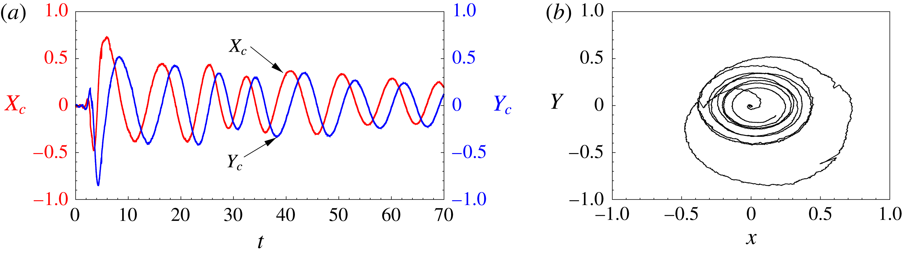
. Figure 15(a) shows the time history of the location of the vortex centre along the
 $X$
- and
 $Y$
-axes with time for the
 $T=4.8$
NLO-P. It can be observed that the displacement of the vortex centre in the two directions is more accentuated than the situation where the simulations are initiated with the LO-P. The vortex centre follows a spiral trajectory about its original unperturbed location (figure 15
b). Figure 16(b) provides the perturbation vorticity field at various time instants in a cycle of energy fluctuation. Close to the vortex core, the perturbation has a dipolar structure and is dominated by the
 $m=1$
component. Far from the centre, other non-zero wavenumbers become significant as well (figure 12
c). Outside the vortex core region, two vorticity patches can be identified. The strength of the positive vorticity patch is lower than that of the negative one and of the dipole present close to the vortex centre, as is evident from figure 16(b). Thus the perturbation field can be considered as a tripole consisting of a dipole and negative satellite vortex. The tripole rotates around the vortex centre and has a rotation period equal to the time period of energy fluctuation. Interestingly, the angular speed of the vorticity patch that is present outside the vortex core is close to the azimuthal velocity of the base flow at that location. This condition corresponds to the criterion of existence of critical layers in shear flows. In a critical layer, the nonlinear terms and/or the viscosity of the flow are significant and allow one to deal with singularities of an otherwise inviscid description of the flow. Habermann (Reference Habermann1972) gave a criterion to distinguish between nonlinear and linear critical layers. As per the criterion, a critical layer is nonlinear if
 $\unicode[STIX]{x1D716}^{3/2}Re\gg 1$
;
 $\unicode[STIX]{x1D716}$
is a measure of the perturbation amplitude and
 $Re$
is the Reynolds number. If
 $\unicode[STIX]{x1D716}^{3/2}Re\ll 1$
, the critical layer is of the viscous type. For
 $\unicode[STIX]{x1D716}^{3/2}Re\sim 1$
, both nonlinear and viscous effects are significant in the critical layer. We use the Habermann criterion to identify the nature of the critical layer in figure 16. The tripolar perturbation structure is observed after the perturbation reaches its peak energy. Therefore, it is reasonable to assume that
 $\unicode[STIX]{x1D716}\sim O(100)$
. Consequently,
 $\unicode[STIX]{x1D716}^{3/2}Re\sim O(10^{5})$
: the critical layer observed in figure 16 is nonlinear. We suspect that the long-term persistence of the energy fluctuation might be attributed to the role of the nonlinear critical layer. This, however, has not been investigated further as part of the present work.
4 Vortex pair
Our principal objective for investigating optimal perturbation of an isolated vortex is its possible application in hastening the decay of aircraft trailing vortices. In general, a trailing vortex system consists of a pair of counter-rotating vortices (in some situations there can be additional vortices). It has been shown in earlier studies that a vortex can experience significant modification to its shape under the strain field of its counter-rotating pair. A question that then arises is: Can the optimization results for isolated vortex be extended to counter-rotating vortex air? We explore the answer to this question by carrying out linear and nonlinear optimization of a vortex pair.
4.1 Base flow
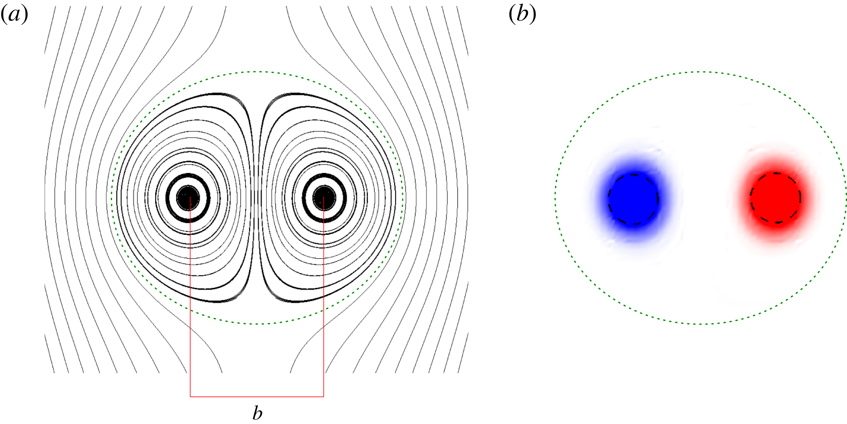
Results for
 $Re=1000$
vortex pair: (a) streamlines and (b) vorticity field for the base flow. The Kelvin oval is indicated using dotted lines in the two panels. The vortex separation is denoted by
 $b$
. The approximate boundary of the two vortex core regions is indicated by a dashed circle in (b). The radius of the circle is equal to the vortex dispersion radius calculated using (3.3).

The base flow is a pair of equal-strength, counter-rotating vortices. The base flow is created by initializing the flow with a pair of counter-rotating Lamb–Oseen vortices and letting it evolve for some time. Since the Lamb–Oseen vortex pair is not a solution of the Navier–Stokes equations, this evolution allows the flow to adjust. During this transient period, the shape of the vortices changes from axisymmetric to elliptic. The flow then evolves on a diffusive time scale. This approach has been used in earlier works on counter-rotating vortex pairs (Sipp, Jacquin & Cossu Reference Sipp, Jacquin and Cossu2000; Brion Reference Brion2009). Owing to its symmetry, we consider only one side of the flow for characterizing the vortex pair. Let the half-domain on the side of the anticlockwise-rotating vortex (positive vorticity) be denoted by
 $\unicode[STIX]{x1D6FA}^{+}$
. The location of the vortex centre, with respect to any origin, is given by
 $$\begin{eqnarray}\displaystyle \boldsymbol{r}_{\boldsymbol{c}}=\frac{\displaystyle \int _{\unicode[STIX]{x1D734}^{+}}\boldsymbol{r}\unicode[STIX]{x1D714}\,\text{d}\unicode[STIX]{x1D734}}{\unicode[STIX]{x1D6E4}}, & & \displaystyle\end{eqnarray}$$
where
 $\boldsymbol{r}$
is the position vector with reference to the same origin. The circulation (
 $\unicode[STIX]{x1D6E4}$
) and vortex dispersion radius (
 $a$
) are given by (3.2) and (3.3), respectively, where the domain of integration is
 $\unicode[STIX]{x1D6FA}^{+}$
. Because of self-induction, the vortex pair translates at a speed equal to
 $\unicode[STIX]{x1D6E4}/2\unicode[STIX]{x03C0}b$
, where
 $b$
is the distance between the two vortex centres. The simulations have been carried out in a frame of reference that moves with the vortex pair. Uniform velocity of magnitude
 $\unicode[STIX]{x1D6E4}/2\unicode[STIX]{x03C0}b$
is specified at the inlet boundary and a stress-free condition is imposed on the outflow and side boundaries. As for the isolated vortex, the base flow for the analysis of the vortex pair is assumed to be frozen. The ratio between the vortex dispersion radius and the separation between vortex centres is
 $a/b\sim 0.18$
. The length and velocity scales have been rendered non-dimensionalized using
 $b$
and
 $\unicode[STIX]{x1D6E4}/2\unicode[STIX]{x03C0}$
. The Reynolds number for all vortex-pair simulations is
 $Re=(\unicode[STIX]{x1D6E4}/2\unicode[STIX]{x03C0}\unicode[STIX]{x1D708})=1000$
. Figure 17 shows the streamlines and the vorticity field for the base flow. Two flow regions can be identified in figure 17. In the first region, the streamlines are closed. In the second region, the flow has an open trajectory. The two flow regions are separated by a limiting streamline referred to as the Kelvin oval.
4.2 Linear optimization
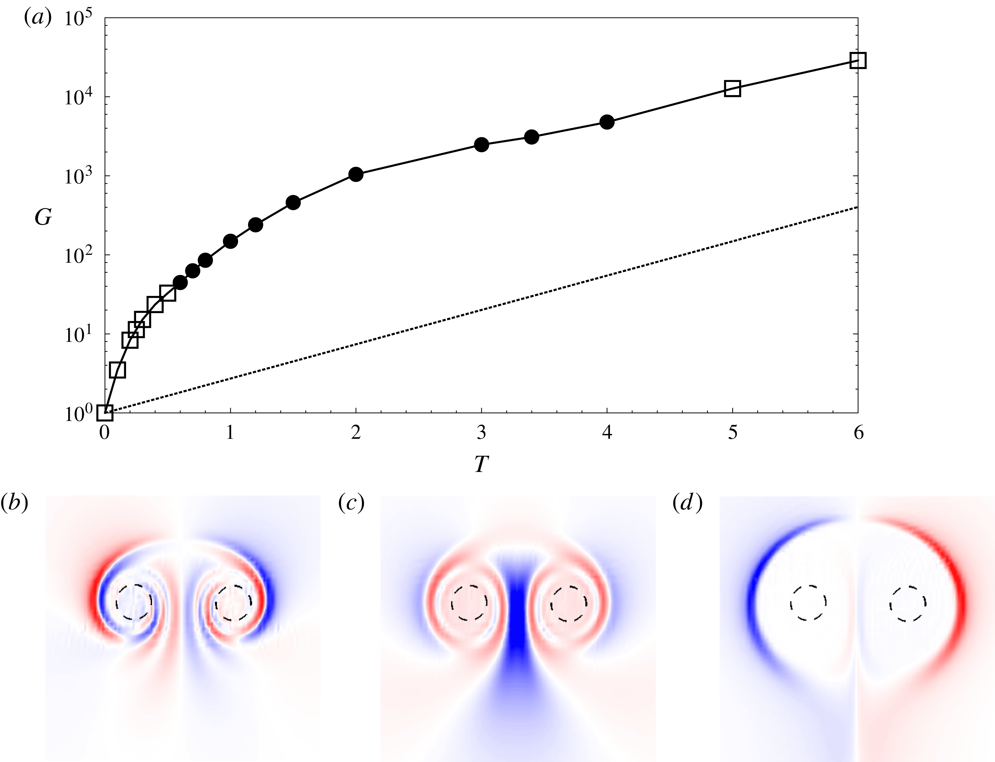
Results for
 $Re=1000$
vortex pair: (a) variation of the linear optimal gain with horizon time. The gain obtained using the most unstable mode as the initial perturbation is indicated by a dotted line. The bottom row shows the velocity component parallel to the centreline for the LO-P corresponding to (b)
 $T=0.5$
, (c)
 $T=1.0$
and (d)
 $T=5.0$
. The solid circles (respectively hollow squares) in (a) correspond to data points for which the LO-P is symmetric (respectively antisymmetric).

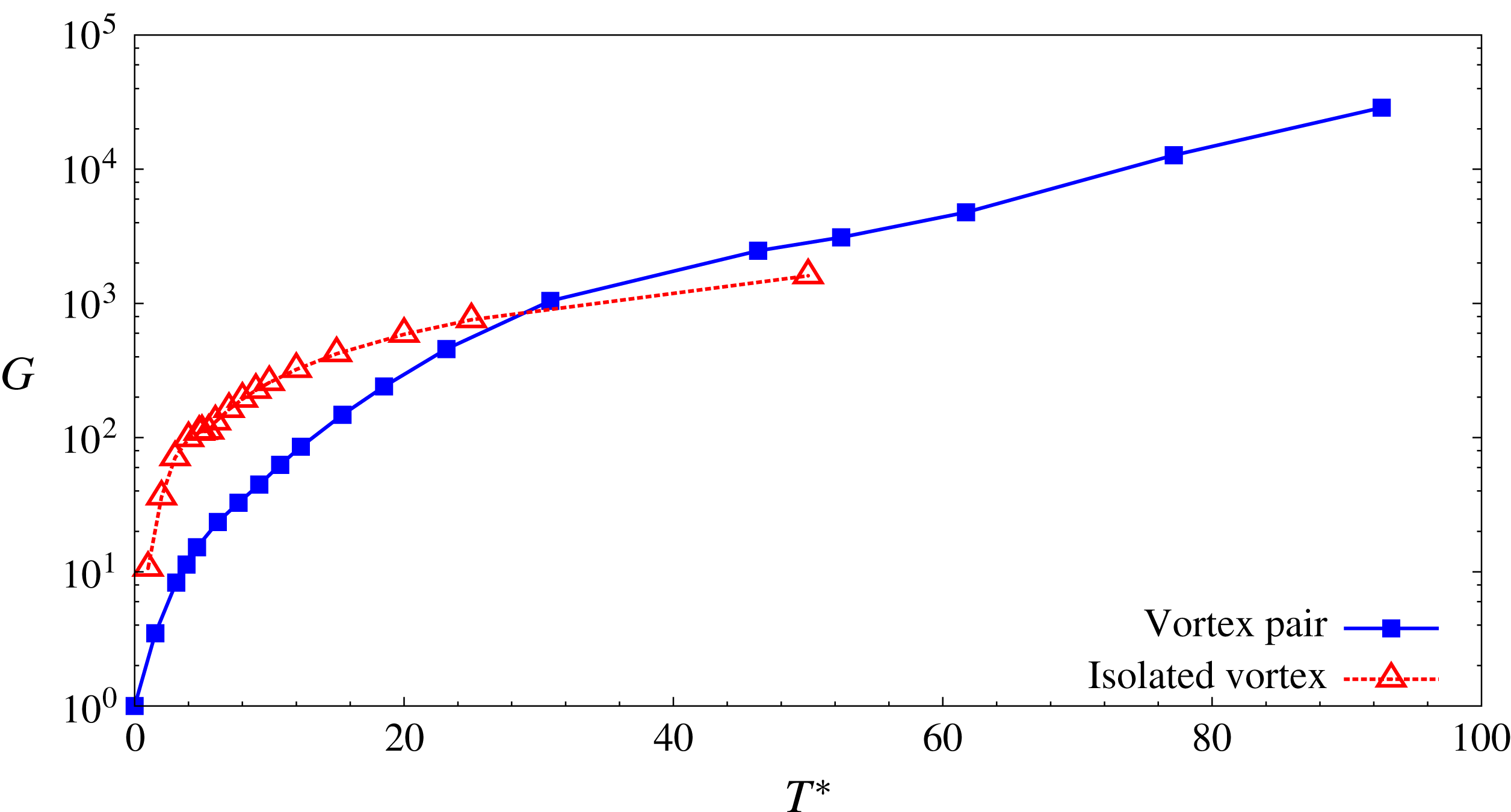
Results for
 $Re=1000$
vortex pair: variation of the LO-G with horizon time rendered non-dimensional by the rotation period of the vortex. Also shown is the LO-G curve for an isolated vortex for
 $Re=5000$
.

Unlike the single-vortex system, a pair of 2D counter-rotating vortices is linearly unstable (Brion et al.
Reference Brion, Sipp and Jacquin2014). In the long term, the most unstable mode will dominate the perturbation evolution. However, before the exponential behaviour sets in, transient (algebraic) growth of perturbation energy may occur due to the non-normality of the linearized Navier–Stokes operator. Therefore, it is possible that for some initial perturbations the energy gain at a given horizon time is higher than the gain obtained using the most unstable mode as the initial perturbation (see appendix B). For the optimization process, as the computations are carried out in the moving reference frame, homogeneous Dirichlet boundary conditions are specified at the inlet and a stress-free condition is applied at the outflow and side boundaries for the direct equations. For the adjoint equations, a homogeneous Dirichlet boundary condition is applied on the outlet and stress-free conditions on the inlet and sidewalls. Figure 18(a) shows the variation of the LO-G with horizon time (
 $T$
) on log–linear axes. Time is rendered non-dimensional using the time taken by a system of two line vortices of strength
 $\pm \unicode[STIX]{x1D6E4}$
to translate a distance equal to
 $b$
under self-induction (
 $\unicode[STIX]{x1D70F}_{b}=2\unicode[STIX]{x03C0}b^{2}/\unicode[STIX]{x1D6E4}$
). Also indicated by a dotted line is the energy gain corresponding to the most unstable mode. It can be observed that the difference between the two gains increases with
 $T$
up to
 $T=4.0$
. For
 $T>4.0$
, LO-G increases exponentially with
 $T$
according to the growth rate of the most unstable mode; the exponential growth appears as a linear curve on log–linear axes. Therefore, the maximum duration for which transient processes contribute to the linear optimal gain is
 $4\unicode[STIX]{x1D70F}_{b}$
.
Any perturbation to a vortex pair can be split into symmetric and antisymmetric components. The velocity field for the (anti)symmetric component is (anti)symmetric about the centreline. Within the linear framework, the two components evolve independently from each other. Therefore, the LO-P can be either symmetric or antisymmetric. A common approach adopted for optimization of a counter-rotating vortex pair is to use half of the computational domain and to prescribe a symmetry or antisymmetry boundary condition on the centreline. In this approach, symmetric and antisymmetric LO-P are obtained separately. We have used a different approach where computations are carried out for the full computational domain. This is because of the unavailability of an antisymmetry boundary condition in Nek5000. LO-P obtained using the full domain approach is the one that has higher energy gain between symmetric and antisymmetric LO-P. For
 $T<0.6$
and
 $T>4.0$
LO-P is antisymmetric, whereas for
 $0.6\leqslant T\leqslant 4.0$
the LO-P is symmetric. Figure 18(b–d) gives the velocity component normal to the centreline for the LO-P corresponding to three horizon times. With increasing
 $T$
, LO-P moves away from the vortex centre. For large
 $T$
, LO-P is primarily located on the Kelvin oval and along the centreline.
We now compare LO-G for an isolated vortex and vortex pair. To do so, we chart the variation of the LO-G with
 $T^{\ast }$
on log–linear axes where
 $T^{\ast }$
is the horizon time rendered non-dimensional by the rotation time of a vortex (
 $T^{\ast }=T\unicode[STIX]{x1D70F}_{b}/\unicode[STIX]{x1D70F}$
and
 $\unicode[STIX]{x1D70F}=4\unicode[STIX]{x03C0}^{2}a^{2}/\unicode[STIX]{x1D6E4}$
) in figure 19. The LO-G curve for the isolated vortex presented earlier (see § 3.2) is included in figure 19. Since, for a vortex pair,
 $G$
increases exponentially with
 $T$
for large
 $T$
(figure 18
a), the same variation is observed in the
 $G$
–
 $T^{\ast }$
curve for large
 $T^{\ast }$
. In figure 19, the exponential behaviour for the vortex pair sets in for
 $T^{\ast }\gtrsim 60$
. For
 $T^{\ast }\lesssim 60$
, the variation of
 $G$
with
 $T^{\ast }$
for the vortex pair is qualitatively similar to that of an isolated vortex. Furthermore, for a given
 $T^{\ast }$
, the linear evolutions of the LO-P for the two systems are also similar. We consider linear flow evolution for
 $T^{\ast }=2.5$
LO-P to demonstrate this. The initial perturbation is antisymmetric about the centreline. Figure 20 shows the shape of LO-P and its evolved state at
 $T^{\ast }$
. The LO-P for both isolated and vortex-pair systems consist of vorticity filaments in a spiral arrangement around the vortex core. The evolved perturbation state at
 $T^{\ast }$
has a quadrupolar structure near the vortex centre. Therefore, it appears that the mechanism for the largest gain in perturbation energy for a vortex pair is the same as that of an isolated vortex. In other words, the interaction between the two vortices of the vortex pair has no significant effect on the physical processes that yield the largest energy gain. The same inference is made with flow evolution of symmetric LO-P.
4.3 Nonlinear optimization
Perturbation vorticity field for (a)
 $Re=5000$
isolated vortex and (b)
 $Re=1000$
vortex pair. The left column shows the field corresponding to
 $T^{\ast }\sim 2.5$
LO-P and the right column shows its evolved state at
 $t=T^{\ast }$
.

Results for
 $Re=1000$
vortex pair: variation of (a) the nonlinear optimal gain with the initial energy of the perturbation for different horizon times,
 $T=0.3$
(○),
 $T=0.5$
(●),
 $T=0.6$
(▵),
 $T=0.8$
(▫),
 $T=1.0$
(▿),
 $T=1.2$
(▪) and
 $T=2.0$
(▴); and (b) the horizon time for
 $E(0)=0.05$
.

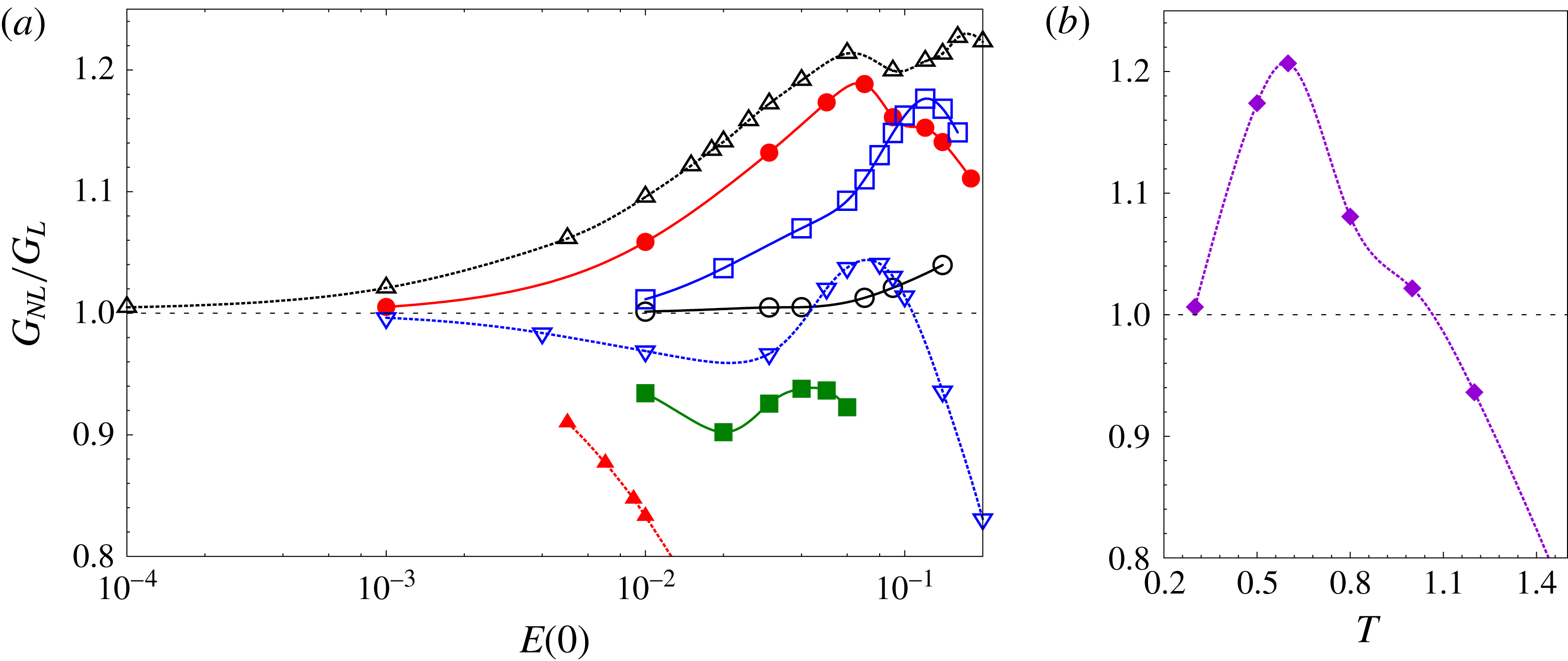
Figure 21 shows the variation of the NLO-G with initial energy of the perturbation (
 $E(0)$
) for various horizon times. NLO-G has been normalized using the LO-G. As for the isolated vortex, there exists a threshold value of
 $E(0)$
below which NLO-G is nearly the same as the LO-G. Above this threshold, the optimal gain is different from the LO-G. With increasing
 $T$
, the threshold
 $E(0)$
decreases. The peak difference between the nonlinear and linear optimal gains increases with horizon time up to
 $T=0.6$
(figure 21
b). For
 $T=0.6$
, the NLO-G is higher than the LO-G for the largest range of
 $E(0)$
. For
 $T>1.0$
, the NLO-G is lower than the LO-G for all the values of
 $E(0)$
that were considered in this work.
Results for
 $Re=1000$
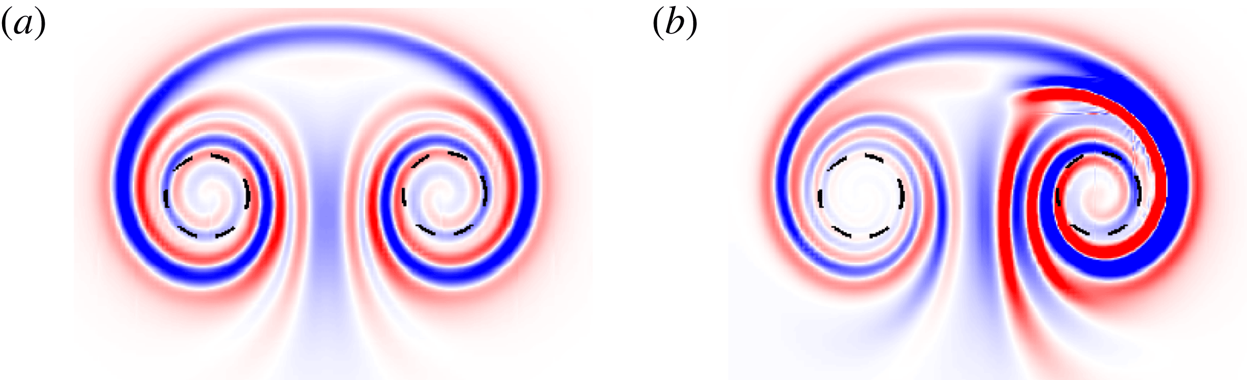
vortex pair: perturbation vorticity field of the
 $T=0.6$
nonlinear optimal perturbation for (a)
 $E(0)=10^{-4}$
and (b)
 $E(0)=0.02$
.

Next we discuss the shape of the NLO-P for a vortex pair. Figure 22 shows the vorticity field of the
 $T=0.6$
nonlinear optimal perturbation for
 $E(0)=10^{-4}$
and
 $E(0)=2\times 10^{-2}$
. The threshold energy for
 $T=0.6$
is
 $E(0)=6\times 10^{-4}$
. Below the threshold energy, the nonlinear and linear optimal perturbations have identical shape. Above the threshold energy, the nonlinear optimal perturbation has an asymmetric structure: the perturbation is stronger in the positive vortex than in the negative vortex.
4.4 Long-term nonlinear evolution of the optimal perturbation
Results for
 $Re=1000$
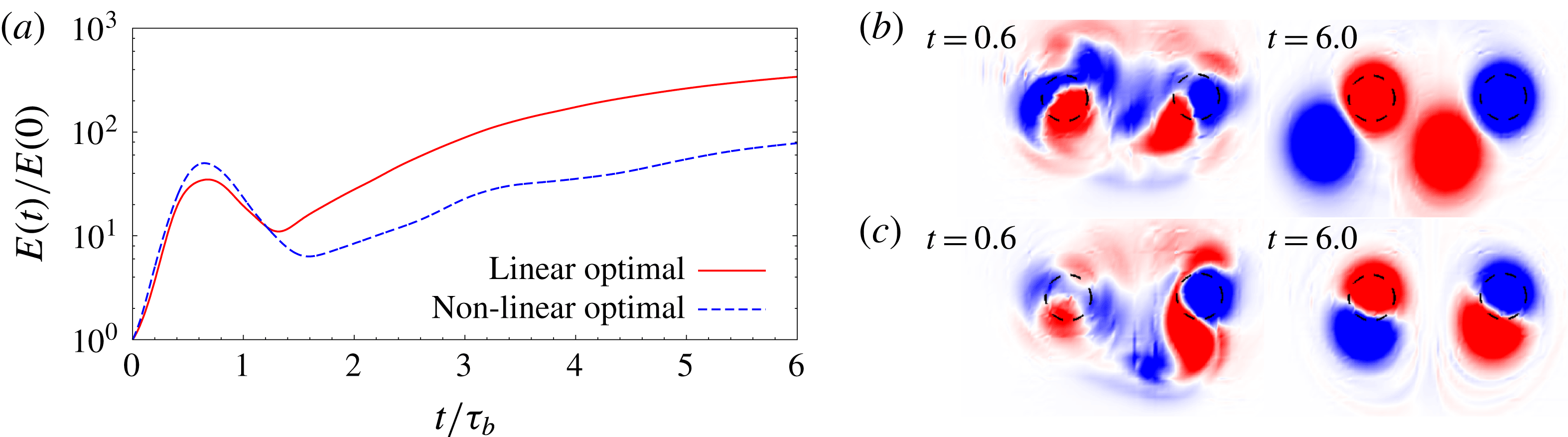
vortex pair: (a) time evolution of the energy gain for computations initiated with the LO-P and the
 $E(0)=0.02$
nonlinear optimal perturbation. (b) Perturbation vorticity field at
 $t=0.6$
and
 $t=6.0$
for the computation initiated with the LO-P. (c) Perturbation vorticity field at
 $t=0.6$
and
 $t=6.0$
for the computation initiated with the
 $E(0)=0.02$
nonlinear optimal perturbation.

Figure 23 gives the time history of the energy gain for computations initiated with the LO-P and the
 $E(0)=0.02$
NLO-P for
 $T=0.6$
. The initial energy of the LO-P is also set to
 $E(0)=0.02$
. Initially, the perturbation energy increases because of the transient processes. The peak gain reached during the transient phase for NLO-P is higher than that reached by the LO-P. In the long term, the LO-P results in higher energy gain than the NLO-P. The perturbation vorticity field at two time instants during the flow evolution are shown in figure 23(b,c). For the LO-P, the flow field at
 $t=T$
is nearly symmetric; whereas for the nonlinear optimal, the flow field is asymmetric. At large times (
 $t=6$
), the perturbation has a dipolar structure near the vortex core. The vortex dipoles provoke a displacement of the vortex cores in the left and downwards direction.
5 Conclusions
Results have been presented for the optimal perturbation of single- and double-vortex systems. The optimal perturbation corresponds to the initial condition that results in largest gain of perturbation energy for a given horizon time
 $T$
. A direct-adjoint approach is employed to compute the optimal perturbations and corresponding gains. Both linear and nonlinear optimizations have been performed.
The single-vortex system is modelled as an isolated 2D Lamb–Oseen vortex. The Reynolds number based on the vortex circulation is
 $Re=5000$
. Linear analysis showed that the optimal perturbation for low horizon time
 $T$
is of azimuthal wavenumber
 $m\geqslant 2$
. For large
 $T$
, the linear optimal perturbation (LO-P) is of
 $m=1$
. In general, LO-P consists of vorticity filaments in a spiral arrangement. With increasing horizon time
 $T$
, the vorticity filaments move away from the vortex centre. For low values of the initial perturbation energy (
 $E(0)$
), linear and nonlinear optimal analyses yield the same result. However, beyond a threshold value of
 $E(0)$
, the nonlinear optimal perturbation (NLO-P) and the corresponding gain are different from those obtained via linear computation. Fourier decomposition of the NLO-P beyond the threshold energy shows contributions from multiple azimuthal wavenumbers. The interaction between different wavenumbers results in higher optimal gain than that of the linear optimal for a range of
 $E(0)$
.
Long-term nonlinear evolution of linear and nonlinear optimal perturbations is studied. It is observed that, after the transient energy growth, the perturbation relaxes towards a quasi-steady non-axisymmetric state. The shape of the perturbation in the quasi-steady state depends on the structure of the optimal perturbation. For example, for the
 $T=4.8$
linear optimal perturbation, the quasi-steady state consists of six vorticity patches; while for the
 $T=4.8$
NLO-P, the quasi-steady state has a tripolar structure. In the tripolar structure, a satellite vortex rotates around a vortex dipole. The appearance of the satellite vortex is attributed to a nonlinear critical layer effect. The optimal perturbations, linear and nonlinear, are a good initial condition to obtain non-axisymmetric vortices.
The two-vortex system has been modelled as a pair of equal-strength counter-rotating vortices. Such a flow configuration is relevant for the study of vortex dynamics in the wake of an aircraft. A counter-rotating vortex pair is a linearly unstable flow system (Brion et al.
Reference Brion, Sipp and Jacquin2014). However, it supports transient growth of perturbation energy that may lead to significantly higher energy gain than that reached by the most unstable mode. For small and large horizon times
 $T$
, the LO-P of a vortex pair is antisymmetric about the centreline; whereas for moderate
 $T$
, the LO-P is symmetric. It is observed that for 2D perturbations, the mechanism of transient growth in a vortex pair is similar to that of an isolated vortex. Adding a counter-rotating vortex in the vicinity of the first vortex does not have a significant effect on the shape of the optimal perturbation within the first vortex. Similarly to the isolated vortex, a threshold value of
 $E(0)$
exists beyond which the nonlinear optimal gain is higher than the linear optimal gain. In this situation the NLO-P is asymmetric about the centreline.
Acknowledgements
We are grateful to Dr M. Farano, DMMM, Politecnico di Bari, Italy, for his help in developing the numerical optimization tool. We would also like to thank Professor P. Brancher, IMFT, Toulouse, for his support and sharing Luigi Bisanti’s experience on nonlinear optimization. This work has been supported by the French Ministry of Civil Aviation (DGAC) under the PHYWAKE (Physics of Wake Vortices) research programme. We thank the anonymous referees for their valuable feedback and insightful suggestions.
Appendix A. Validation of the frozen base-flow approach
In this appendix, the validity of the frozen base-flow approach for linear and nonlinear optimization processes is demonstrated. We select
 $T=4.8$
and compute the nonlinear and linear optimal gains with frozen as well as diffusing base flow. Table 2 lists the values of the optimal gain obtained via the two approaches. It can be observed that the difference between the two approaches is less than 0.5 %. The slightly lower value of optimal gain obtained using diffusing base flow is attributed to reduction of vortex strength under the action of viscosity.
Linear and nonlinear
 $E_{0}=10^{-2}$
optimal gains
 $G(T)$
obtained for a Lamb–Oseen vortex at
 $Re=5000$
, with
 $T=4.8$
using a frozen base flow and a diffusing base flow.

Appendix B. Vortex pair: contribution of most unstable mode to LO-P
Value of
 $C_{mum}$
(defined by (B 1)) calculated for LO-P corresponding to various horizon times.

A pair of counter-rotating planar vortices is a linearly unstable flow system (Brion et al. Reference Brion, Sipp and Jacquin2014). The long-time response of the linearized system will be governed by the most unstable mode. However, owing to the non-normal nature of the linearized operator, the most unstable mode alone cannot be representative of short-time transient flow processes. To confirm this, we calculate the following ratio for LO-P computed for various horizon times:
 $$\begin{eqnarray}\displaystyle C_{mum}(T)=\frac{(\boldsymbol{u}_{\boldsymbol{o}\boldsymbol{p}\boldsymbol{t}}(\boldsymbol{T}),\boldsymbol{u}_{\boldsymbol{m}}^{+})}{(\boldsymbol{u}_{\boldsymbol{m}},\boldsymbol{u}_{\boldsymbol{m}}^{+})}. & & \displaystyle\end{eqnarray}$$
In (B 1), the numerator on the right-hand side is the scalar product between the velocity field corresponding to linear optimal perturbation (
 $\boldsymbol{u}_{\boldsymbol{o}\boldsymbol{p}\boldsymbol{t}}$
), and the adjoint of the most unstable mode of the vortex-pair system (
 $\boldsymbol{u}_{\boldsymbol{m}}^{+}$
). The denominator on the right-hand side of (B 1) is the scalar product between the most unstable mode (
 $\boldsymbol{u}_{\boldsymbol{m}}$
) and
 $\boldsymbol{u}_{\boldsymbol{m}}^{+}$
. In the calculation of the scalar product, only spatial integration is carried out (unlike the inner product defined in (2.9), where the integration is carried out in both space and time), and all the vectors are normalized with respect to their norm. The ratio
 $C_{mum}$
is a measure of the contribution of the most unstable mode (
 $mum$
) to LO-P. This follows from the bi-orthogonality relation between the eigenmodes of the direct and adjoint systems. Table 3 shows the value of
 $C_{mum}$
calculated for LO-P corresponding to various horizon times. For large
 $T$
,
 $C_{mum}$
is relatively high. This suggests a large contribution of the most unstable mode in long-time LO-P. On the other hand, for low
 $T$
, the contribution of the most unstable mode to LO-P is low, as evidenced by the relatively small value of
 $C_{mum}$
.