2 Modulated nearly monochromatic beams

As in KA, the present analysis assumes an unbounded, incompressible, uniformly stratified Boussinesq fluid with (constant) buoyancy frequency $N$ . Here, we also include the effect of background rotation, which is physically important in geophysical settings due to the Earth’s rotation and, moreover, brings out the pivotal role of potential vorticity (PV) in inducing streaming. With $1/N$ as time scale and $L_{\ast }=\unicode[STIX]{x1D706}_{\ast }/2\unicode[STIX]{x03C0}$ (where $\unicode[STIX]{x1D706}_{\ast }$ is the packet carrier wavelength) as length scale, the non-dimensional governing equations for the velocity field $\boldsymbol{u}$ , the reduced density $\unicode[STIX]{x1D70C}$ and pressure  $p$  are

Here, $\text{D}/\text{D}t\equiv \left.\unicode[STIX]{x2202}/\unicode[STIX]{x2202}t\right.+\boldsymbol{u}\boldsymbol{\cdot }\boldsymbol{\unicode[STIX]{x1D6FB}}$ is the material derivative, $\boldsymbol{j}$ is a vertical unit vector pointing upwards, $\boldsymbol{f}=f\boldsymbol{j}$ , where $f$ is the local Coriolis parameter normalized with $N$ , and $\unicode[STIX]{x1D708}=\unicode[STIX]{x1D708}_{\ast }/NL_{\ast }^{2}$ is the inverse Reynolds number, where $\unicode[STIX]{x1D708}_{\ast }$ denotes the kinematic viscosity.

Under the assumed flow conditions, it follows from (2.1) that

where

denotes the (non-dimensional) PV. According to (2.2), $q$ is a materially conserved quantity in the absence of dissipation ( $\unicode[STIX]{x1D708}=0$ ). Furthermore, in the linear limit, gravity–inertia internal waves are entirely decoupled from the vortical mode of motion that carries all the flow PV (e.g. Müller Reference Müller1995). For weakly nonlinear internal wavepackets in a viscous fluid, however, as argued below, the nonlinear dissipative term on the right-hand side of (2.2) is capable of producing mean PV, which translates into streaming.

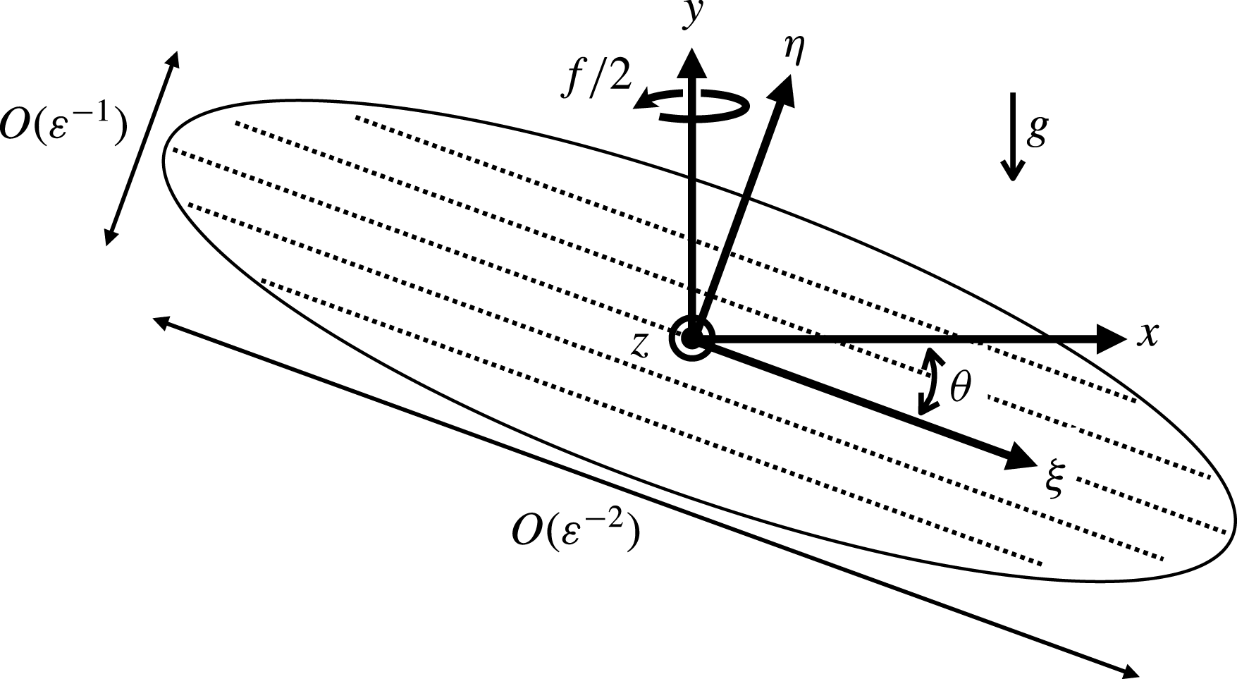
The governing equations (2.1) for $\unicode[STIX]{x1D708}=0$ support time-harmonic plane waves in the form of beams (Tabaei & Akylas Reference Tabaei and Akylas2003). These states feature a general profile in the cross-beam ( $\unicode[STIX]{x1D702}$ -) direction, and are uniform in the along-beam ( $\unicode[STIX]{x1D709}$ -) and the transverse horizontal ( $z$ -) direction (figure 1). Specifically, the beam velocity components $\boldsymbol{u}=(u,v,w)$ in the coordinate system $(\unicode[STIX]{x1D709},\unicode[STIX]{x1D702},z)$ are given by

where $A(\unicode[STIX]{x1D702})$ is a general profile, and the frequency $\unicode[STIX]{x1D714}$ is tied to the beam inclination $\unicode[STIX]{x1D703}$ to the horizontal, via the dispersion relation

Figure 1.

Schematic of modulated nearly monochromatic beam of carrier frequency $\unicode[STIX]{x1D714}$ and inclination $\unicode[STIX]{x1D703}$ to the horizontal, in keeping with (2.5). The coordinate system $(\unicode[STIX]{x1D709},\unicode[STIX]{x1D702},z)$ is defined by the along-beam, cross-beam and transverse directions, respectively. Dotted lines indicate lines of constant phase of the sinusoidal carrier, which is modulated by a three-dimensional slowly varying envelope. Measured in terms of the carrier wavelength (normalized to $2\unicode[STIX]{x03C0}$ ), the envelope scale is $O(\unicode[STIX]{x1D700}^{-2})$ along the $\unicode[STIX]{x1D709}$ - and $O(\unicode[STIX]{x1D700}^{-1})$ along the $\unicode[STIX]{x1D702}$ - and $z$ -directions.

Starting from the inviscid uniform state (2.4) (for $f=0$ ), KA developed an asymptotic model for the propagation of a weakly nonlinear, slightly viscous beam with long-scale variations in $\unicode[STIX]{x1D709}$ and $z$ relative to the beam width. This analysis assumed a general beam profile $A(\unicode[STIX]{x1D702})$ with $O(1)$ width in $\unicode[STIX]{x1D702}$ . By contrast, the focus here is on beams whose profile comprises a sinusoidal carrier, $A(\unicode[STIX]{x1D702})\propto \exp (\text{i}\unicode[STIX]{x1D702})$ , modulated by a three-dimensional slowly varying envelope (figure 1); such disturbances will be referred to as modulated nearly monochromatic beams (MNMB).

Several earlier analyses of wave–mean-flow interaction (e.g. Grimshaw Reference Grimshaw1979; Bühler & McIntyre Reference Bühler and McIntyre1998; Grisouard & Bühler Reference Grisouard and Bühler2012) used the generalized Lagrangian-mean (GLM) formalism (Andrews & McIntyre Reference Andrews and McIntyre1978). Instead, we shall work directly with (2.1) and the associated PV equation (2.2), employing weakly nonlinear multiple-scale expansions. In setting up the present model, the first step is to specify the envelope scales. To this end, we define $\unicode[STIX]{x1D700}\ll 1$ as the ratio of the carrier wavelength to the transverse beam length scale; thus, the transverse envelope variable is

Then, we balance the transverse dispersion with the along-beam dispersion and the viscous decay of the beam. As in KA, this is achieved by employing the following stretched along-beam coordinate, slow time and scaled inverse Reynolds number

where $\unicode[STIX]{x1D6FD}=O(1)$ . Finally, in regard to the cross-beam ( $\unicode[STIX]{x1D702}$ -) envelope scale, we expect cross-beam modulations to affect only the beam–mean-flow coupling, as uniform beams are exact nonlinear solutions of (2.1) (for $\unicode[STIX]{x1D708}=0$ ) irrespective of the profile $A(\unicode[STIX]{x1D702})$ in (2.4). Also, according to KA, a beam of $\unicode[STIX]{x1D702}=O(1)$ width and the same modulations as (2.6) and (2.7) induces a mean flow that extends over $\unicode[STIX]{x1D702}=O(1/\unicode[STIX]{x1D700})$ . This suggests taking

as cross-beam envelope variable, to ensure optimal coupling of a MNMB with its induced mean flow; moreover, as will be verified later (2.17), this choice avoids the inner–outer mean-flow analysis of KA.

To complete the scalings of our model, it remains to specify the beam amplitude, which controls nonlinearity, and the relative magnitude of the induced mean flow. Our interest centres on the ‘distinguished limit’ where the effects of nonlinearity formally have equal weight and act on the same slow time $T=\unicode[STIX]{x1D700}^{2}t$ as dispersion and dissipation. More specifically, suppose the beam peak amplitude is $O(\unicode[STIX]{x1D6FC})$ , with $\unicode[STIX]{x1D6FC}\ll 1$ to be related to $\unicode[STIX]{x1D700}$ ,

where $\unicode[STIX]{x1D719}=\unicode[STIX]{x1D702}-\unicode[STIX]{x1D714}t$ and $U,V,W,R$ and $P$ are functions of $\boldsymbol{X}=(X,Y,Z)$ and $T$ . Then, from (2.1a,b ) and the $\unicode[STIX]{x1D702}$ - and $z$ -components of (2.1c ), to leading order,

Looking next at the $\unicode[STIX]{x1D709}$ -component of (2.1c ), by virtue of (2.5) and (2.10), the leading-order terms cancel out as expected, and the slow-time evolution term $\unicode[STIX]{x1D700}^{2}\unicode[STIX]{x1D6FC}U_{T}\exp (\text{i}\unicode[STIX]{x1D719})$ is as important as the leading-order mean-flow interaction term $\text{i}\unicode[STIX]{x1D6FC}\overline{v}U\exp (\text{i}\unicode[STIX]{x1D719})$ if the cross-beam ( $\unicode[STIX]{x1D702}$ -) mean flow $\overline{v}(\boldsymbol{X},T)=O(\unicode[STIX]{x1D700}^{2})$ . Furthermore, from the mean-flow analysis of KA which employed the same scalings $\boldsymbol{X}$ and $T$ , we expect the along-beam ( $\unicode[STIX]{x1D709}$ -) and transverse ( $z$ -) mean flows to be comparable to $\overline{v}$ : $\overline{u}(\boldsymbol{X},T)\sim \overline{w}(\boldsymbol{X},T)=O(\unicode[STIX]{x1D700}^{2})$ . As a result, according to (2.3), the induced mean PV, $\overline{q}(\boldsymbol{X},T)=f+O(\unicode[STIX]{x1D700}^{3})$ , so the slow-time evolution term $\unicode[STIX]{x1D700}^{2}\overline{q}_{T}$ on the left-hand side of the PV equation (2.2) is $O(\unicode[STIX]{x1D700}^{5})$ . Turning next to the production of mean PV on the right-hand side of (2.2), by making use of (2.9) and (2.10) this term is found to be $O(\unicode[STIX]{x1D708}\unicode[STIX]{x1D6FC}^{2}\unicode[STIX]{x1D700})$ , that is $O(\unicode[STIX]{x1D6FC}^{2}\unicode[STIX]{x1D700}^{3})$ in view of (2.7); hence, the time rate of change of $\overline{q}$ is compatible with the production of $\overline{q}$ when the amplitude parameter $\unicode[STIX]{x1D6FC}=\unicode[STIX]{x1D700}$ .

The above qualitative discussion suggests the following expansions

where all primary-harmonic and mean-flow amplitudes are functions of $\boldsymbol{X}$ and $T$ . Inserting these expansions into (2.1), we first focus on terms that contribute to the primary harmonic, correct to $O(\unicode[STIX]{x1D700}^{3})$ . Similar to the approach leading to (2.10), we use (2.1a,b ) and the $\unicode[STIX]{x1D702}$ - and $z$ -components of (2.1c ) to solve for $V,W,R$ and $P$ in terms of $U$ . Combining these results with the $\unicode[STIX]{x1D709}$ -component of (2.1c ) then yields the following evolution equation for $U$

where

In (2.12), the feedback of the wave-induced mean flow onto the wave beam itself is communicated via the action of the cross-beam ( $\unicode[STIX]{x1D702}$ -) mean flow $\overline{V}$ , to be determined below. Additionally, as expected for a MNMB, the wave envelope $U$ does not feel the effect of cross-beam ( $Y$ -) modulations except through the nonlinear mean-flow feedback.

Turning next to the mean-flow terms, according to (2.1b ), $\overline{U}\sin \unicode[STIX]{x1D703}-\overline{V}\cos \unicode[STIX]{x1D703}=O(\unicode[STIX]{x1D700})$ ; thus, the mean flow is purely horizontal to leading order. Furthermore, from (2.1a,c ), to leading order, $\overline{W}_{Z}=-\overline{V}_{Y},\overline{R}_{Z}=-f\cot \unicode[STIX]{x1D703}\,\overline{V}_{Y},\overline{P}_{Z}=f\csc \unicode[STIX]{x1D703}\,\overline{V}$ ; the latter two relations are expressions of the vorticity equation (the ‘thermal wind’ equation) and geostrophic balance, respectively. It remains to derive an evolution equation for $\overline{V}$ . To this end, while it is possible to proceed directly from (2.1), we instead find it more instructive to appeal to the PV equation (2.2). Specifically, upon substituting expansions (2.11) into (2.2) and (2.3) and collecting primary-harmonic and mean terms, it follows that

where

and $Q=-\text{i}\unicode[STIX]{x1D6FD}f\sin 2\unicode[STIX]{x1D703}\,U/2\unicode[STIX]{x1D714}^{2}+O(\unicode[STIX]{x1D700})$ . The first term on the right-hand side of (2.14) represents the constant planetary vorticity and, as it plays no role in PV evolution, has been separated from the rest of the mean PV, which is governed by

This brings out the vital role of dissipation combined with nonlinearity, the latter being brought about by the presence of transverse ( $z$ -) variations, in producing mean PV. Finally, inserting (2.15) in (2.16) and using $\overline{W}_{Z}=-\overline{V}_{Y}+O(\unicode[STIX]{x1D700})$ , we find

where $\unicode[STIX]{x1D6FF}=2\sin ^{2}\unicode[STIX]{x1D703}/\unicode[STIX]{x1D714}$ . Together, (2.12) and (2.17) form a closed system of evolution equations for $U$ and $\overline{V}$ that govern the interaction between a weakly nonlinear MNMB and its induced mean flow. These equations remain valid in the absence of background rotation ( $f=0$ ) even though the scalings introduced earlier assuming $f=O(1)$ need to be slightly modified in the limit $f\ll 1$ (Fan Reference Fan2017).

Equation (2.17) reveals two distinct mean-flow generation mechanisms, associated with: (i) the inviscid, purely modulation-induced term on the left-hand side; and (ii) the viscous driving term appearing on the right-hand side. In the absence of dissipation ( $\tilde{\unicode[STIX]{x1D6FD}}=0$ ), when only (i) is present, (2.17) reduces to a Poisson equation for $\overline{V}$ so the mean-flow dynamics is ‘slaved’ to the beam evolution governed by (2.12). Allowing for dissipation and assuming the beam has reached a quasisteady state (in the presence of external forcing, for instance), (ii) can trigger resonant mean-flow growth (linear in $T$ ), i.e. streaming. In either scenario, transverse ( $Z$ -) modulations are essential, as they produce the non-uniform Reynolds stresses responsible for mean-flow generation. In terms of PV, according to (2.2) and (2.15), the modulation-induced mean flow arises from the material conservation of PV under inviscid flow conditions; streaming, on the other hand, results from the irreversible production of mean PV described by (2.16), as pointed out by McIntyre & Norton (Reference McIntyre and Norton1990).

3 Inviscid stability analysis

According to the interaction equations (2.12) and (2.17), the effect of the induced mean flow is to refract the MNMB. This three-dimensional nonlinear refraction occurs on the same time scale as the envelope propagation, dispersion and viscous damping, so potentially could have significant impact on the beam profile. To address this issue, we first examine the possibility of purely modulation-induced instability of a uniform beam in the inviscid limit ( $\tilde{\unicode[STIX]{x1D6FD}}=0$ ). The role of streaming is discussed in § 4.

For $\tilde{\unicode[STIX]{x1D6FD}}=0$ , equations (2.12) and (2.17) admit solutions in the form $U=U_{B}(Y)$ , $\overline{V}=0$ , which correspond to uniform nearly monochromatic beams with general, locally confined envelope $U_{B}(Y)$ . To examine the linear stability of these states to infinitesimal along-beam and transverse modulations, we introduce perturbations in the form of normal modes,

where $k$ and $m$ are given real wavenumbers and $\unicode[STIX]{x1D70E}$ is an undetermined, possibly complex frequency. Substituting (3.1) into (2.12) and (2.17) (with $\tilde{\unicode[STIX]{x1D6FD}}=0$ ), linearizing with respect to the perturbations and eliminating $\hat{u} _{\pm }$ , we obtain the following eigenvalue problem

with $\unicode[STIX]{x1D6EC}=2\unicode[STIX]{x1D6FE}\unicode[STIX]{x1D6FF}m^{4}/\{(\unicode[STIX]{x1D70E}-c_{g}k)^{2}-\unicode[STIX]{x1D6FE}^{2}m^{4}\}$ as eigenvalue parameter. Upon multiplying (3.2) with $\hat{v}^{\ast }$ , integrating from $-\infty$ to $+\infty$ and making use of (3.3), it follows that

This shows that $\unicode[STIX]{x1D6EC}$ is real and positive for any given $U_{B}(Y)$ . Hence, because $c_{g}$ is real and $\unicode[STIX]{x1D6FE}\unicode[STIX]{x1D6FF}$ is real and positive, $\unicode[STIX]{x1D70E}=c_{g}k\pm m^{2}(\unicode[STIX]{x1D6FE}^{2}+2\unicode[STIX]{x1D6FE}\unicode[STIX]{x1D6FF}/\unicode[STIX]{x1D6EC})^{1/2}$ is purely real, and uniform nearly monochromatic beams are stable in the inviscid limit irrespective of the envelope profile $U_{B}(Y)$ . The inviscid stability analysis can be extended to uniform beams involving multiple collinear carrier wavevectors, in which case stability is no longer guaranteed; purely standing beams, in particular, are always unstable (Fan Reference Fan2017).

4 Effects of streaming

We now assess the effects of streaming, when $\tilde{\unicode[STIX]{x1D6FD}}\neq 0$ , on the evolution of MNMB. Specifically, equations (2.12) and (2.17) are solved numerically assuming a quiescent fluid initially and that waves are generated for $T>0$ , $X>0$ from a locally confined source at $X=0$ , which effectively specifies the envelope profile $U$ there. This model mimics the experimental set-up of Bordes (Reference Bordes2012) and Bordes et al. (Reference Bordes, Venaille, Joubaud, Odier and Dauxois2012), where a mechanical wave generator with sinusoidal vertical profile (carrier wavelength $\unicode[STIX]{x1D706}_{\ast }=3.8$  cm) and limited vertical ( $=3\unicode[STIX]{x1D706}_{\ast }$ ) and transverse ( $=3.7\unicode[STIX]{x1D706}_{\ast }$ ) extent, was placed at one end of a non-rotating ( $f=0$ ) stratified tank ( $N=0.85~\text{rad}~\text{s}^{-1}$ , $\unicode[STIX]{x1D708}_{\ast }=0.9\times 10^{-6}~\text{m}^{2}~\text{s}^{-1}$ ). In non-dimensional variables ( $\unicode[STIX]{x1D706}_{\ast }/2\unicode[STIX]{x03C0}=$ length scale, $1/N=$ time scale), normalizing the transverse width of this wavemaker to $Z=1$ sets $\unicode[STIX]{x1D700}=0.043$ and the viscous parameter $\unicode[STIX]{x1D6FD}=15.6$ according to (2.6) and (2.7); furthermore, the forcing effect of the wavemaker is accounted for by the boundary condition at $X=0$ : $U=A_{0}[\tanh (5(Z+0.5))-\tanh (5(Z-0.5))]\times [\tanh (15(Y+0.4))-\tanh (15(Y-0.4))]/4$ , where $A_{0}$ controls the peak forcing amplitude. The resulting initial–boundary-value problem is solved using pseudo-spectral discretization in $Y\in [-3.4,3.4]$ and $Z\in [-5.4,5.4]$ with $256\times 256$ Fourier modes, third-order upwind finite differencing in $X\in [0,0.14]$ with 500 grid points, and fourth-order Runge–Kutta time stepping with $\unicode[STIX]{x0394}T=2.5\times 10^{-4}$ .

Bordes et al. (Reference Bordes, Venaille, Joubaud, Odier and Dauxois2012) report detailed experimental results for the (dimensionless) driving frequency $\unicode[STIX]{x1D714}=0.26$ ( $\unicode[STIX]{x1D703}\approx 15^{\circ }$ ). The theoretical predictions of KA are in good agreement with these observations despite the fact that the thin-beam assumption (beam width $\ll$ transverse extent) made in KA, which leads to an inner–outer mean-flow structure in the cross-beam ( $\unicode[STIX]{x1D702}$ -) direction, is not met experimentally. The present model, by comparison, treats the beam response as a MNMB (with 3 carrier lengths) and reproduces the results of Bordes et al. (Reference Bordes, Venaille, Joubaud, Odier and Dauxois2012) more accurately, particularly in regard to the observed mean flow which is confined close to the beam in the cross-beam ( $\unicode[STIX]{x1D702}$ -) direction, consistent with the scaling (2.8) (Fan Reference Fan2017).

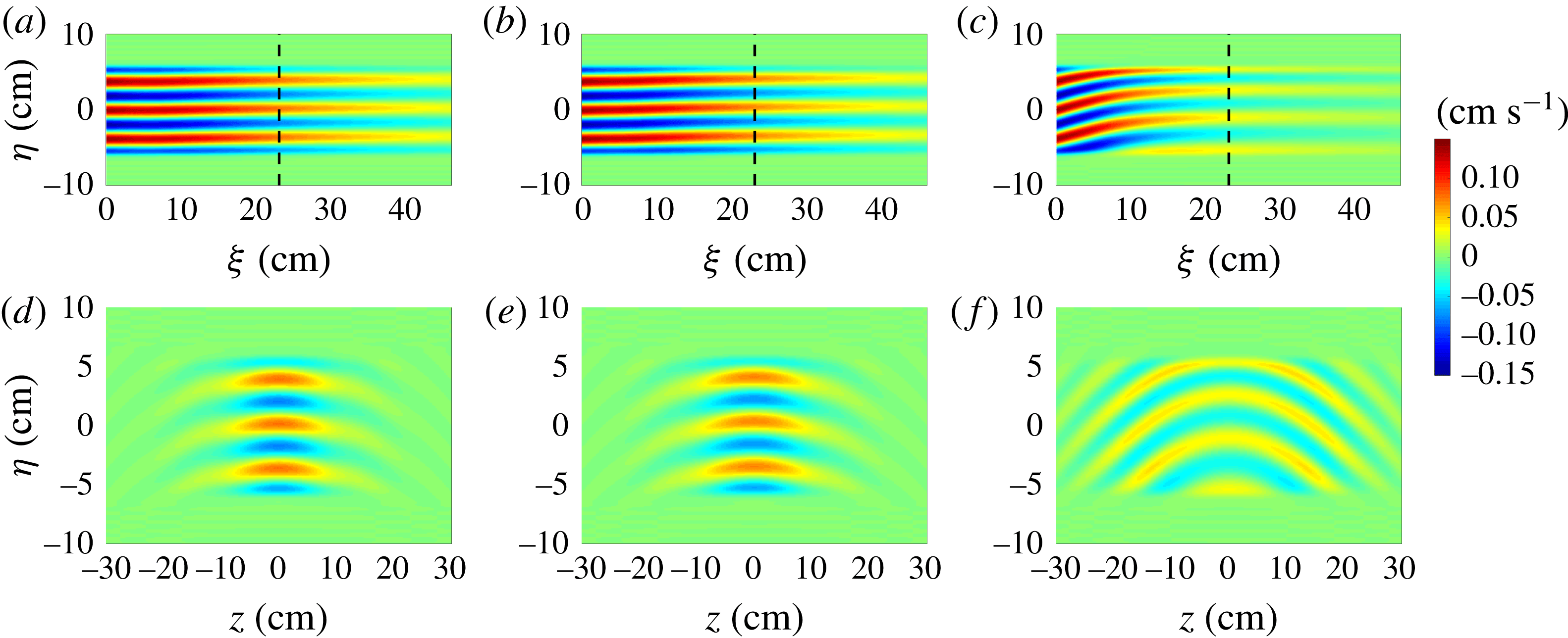
Rather than elaborating on the comparison with Bordes et al. (Reference Bordes, Venaille, Joubaud, Odier and Dauxois2012), we shall focus on $\unicode[STIX]{x1D714}=0.47$ ( $\unicode[STIX]{x1D703}\approx 28^{\circ }$ ) in the light of experimental evidence at this driving frequency (Bordes Reference Bordes2012) that the induced mean flow can have a marked impact on the beam response. Figure 2 shows the horizontal ( $x$ -) velocity of the computed MNMB (including the carrier) for $\unicode[STIX]{x1D714}=0.47$ and $f=0$ at $T=1$ (corresponding to 640 s) according to: (a,d) the linear solution; (b,e) the nonlinear solution ignoring the right-hand side of (2.17) which drives streaming; and (c,f) the nonlinear solution using the full equation (2.17). Here we chose $A_{0}=3.7$ in order to obtain beam velocities comparable to the experimental values, and the plots are in dimensional variables to ease comparison with Bordes (Reference Bordes2012). From figure 2(a,b,d,e), it is clear that the inviscid mean flow has practically no effect on the beam evolution, consistent with the conclusion reached in § 3 that uniform nearly monochromatic beams are stable in the inviscid limit. By contrast, streaming not only bends the beam crests (figure 2 c), but also causes the beam profile to broaden significantly in the transverse ( $z$ -) direction (figure 2 f). To explain this broadening, we note that, because of transverse variations in the beam profile, $\overline{V}$ also varies in the $Z$ -direction. Therefore, $\text{i}\overline{V}U$ , which appears to only act as a refraction term in (2.12), also enhances $Z$ -variations in the beam envelope $U$ and thereby amplifies transverse dispersion. Furthermore, figure 2(a–c) reveals that streaming is also responsible for accelerating the beam decay in the along-beam ( $\unicode[STIX]{x1D709}$ -) direction. This can be understood with the help of the conservation law $E_{T}+c_{g}E_{X}+\tilde{\unicode[STIX]{x1D6FD}}E=0$ , which follows from (2.12) and (2.17) for $E=\int _{-\infty }^{\infty }\left|U\right|^{2}\text{d}Z$ ; thus $E=E_{0}(Y)\text{exp}(-\tilde{\unicode[STIX]{x1D6FD}}X/c_{g})$ for $0\leqslant X<c_{g}T$ and $E=0$ for $X>c_{g}T$ , where $E_{0}=E(X=0)$ is fixed by the wavemaker boundary condition. Remarkably, the evolution of $E$ is oblivious to the beam–mean-flow interaction, so the transverse broadening caused by streaming is compensated by a faster along-beam amplitude decay than that due to viscous damping alone. As an accuracy check, the conservation law for $E$ was satisfied in our simulations with less than $0.2\,\%$ relative error.

Figure 2.

Horizontal ( $x$ -) velocity of computed MNMB (including the carrier) for driving frequency $\unicode[STIX]{x1D714}=0.47$ ( $\unicode[STIX]{x1D703}\approx 28^{\circ }$ ) and no rotation $f=0$ , at $T=1$ (640 s). (a,d) Linear response; (b,e) nonlinear response ignoring the streaming term on the right-hand side of (2.17); and (c,f) nonlinear response using the full equation (2.17). The location of the wavemaker is at $\unicode[STIX]{x1D709}=0$ . Vertical slices (a–c) are taken at $z=0$ , while beam cross-section slices (d–f) are taken at $\unicode[STIX]{x1D709}=23~\text{cm}$ (dotted lines in the a–c).

The streaming effects noted above – cross-beam refraction, transverse broadening and increased along-beam decay of the beam profile – are supported by figure 4.6 of Bordes (Reference Bordes2012), which compares the observed beam response for $\unicode[STIX]{x1D714}=0.47$ at an early time (65 s), prior to significant mean-flow accumulation, with that at a much later stage (1000 s) when streaming is in full effect. Furthermore, according to our model, streaming causes the beam cross-section to develop two maxima far from the wave generator (figure 2 f), also in agreement with figure 4.6 of Bordes (Reference Bordes2012). In spite of this favourable qualitative agreement though, quantitative comparison is not feasible, as the model, from early times, overpredicts (by roughly a factor of two) the streaming induced by a beam of comparable strength to that in the experiment. Given the satisfactory quantitative agreement between theory and experiment for $\unicode[STIX]{x1D714}=0.26$ (Fan Reference Fan2017), we suspect that the discrepancy for $\unicode[STIX]{x1D714}=0.47$ is due to finite-amplitude effects, not captured by our weakly nonlinear model, in the mean-flow evolution. This explanation is bolstered by the stronger beam response and the qualitatively different evolution of the integrated mean vertical vorticity observed experimentally for $\unicode[STIX]{x1D714}=0.47$ in comparison with $\unicode[STIX]{x1D714}=0.26$ (figure 4.4a in Bordes (Reference Bordes2012), reproduced as figure 4a in Bordes et al. (Reference Bordes, Venaille, Joubaud, Odier and Dauxois2012)).

5 MNMB versus round wavepackets

MNMB are characterized by relatively weak modulations in the along-beam ( $\unicode[STIX]{x1D709}$ -) direction, which is also the direction of group velocity (figure 1). As a result, according to (2.12), the propagation of the wave envelope with the group velocity $c_{g}$ takes place on the same slow time $T=\unicode[STIX]{x1D700}^{2}t$ as transverse dispersion, viscous dissipation and refraction by the induced mean flow; moreover, the inviscid, modulation-induced mean flow and the viscous streaming, which evolve on $T$ as well in keeping with (2.17), take part on an equal footing in the wave–mean-flow interaction. For wavepackets with general three-dimensional modulations, however, this distinguished limit cannot be realized, and streaming plays a less prominent role in the interaction dynamics. Here, we illustrate this fundamental difference between MNMB and general wavepackets for the case of a ‘round’ three-dimensional wavepacket whose envelope is modulated isotropically.

Shrira (Reference Shrira1981) discussed the propagation of a round three-dimensional internal wavepacket in an inviscid ( $\unicode[STIX]{x1D708}=0$ ) non-rotating ( $f=0$ ) fluid and derived two coupled evolution equations, analogous to (2.12) and (2.17), for the wave–mean-flow interaction. Specifically, replacing $X=\unicode[STIX]{x1D700}^{2}\unicode[STIX]{x1D709}$ with $\tilde{X}=\unicode[STIX]{x1D700}\unicode[STIX]{x1D709}$ in keeping with the isotropic modulation, the wavepacket envelope propagates along $\tilde{X}$ with the group velocity for $\tilde{T}=\unicode[STIX]{x1D700}t=O(1)$ , while the effects of dispersion and refraction due to the induced mean flow come into play on the slower time scale $T=\unicode[STIX]{x1D700}^{2}t$ as in (2.12). Furthermore, similar to (2.17) for $\tilde{\unicode[STIX]{x1D6FD}}=0$ , the mean flow, which again is driven by transverse ( $Z$ -) modulations, satisfies a Poisson equation, and a uniform wavetrain generally experiences modulation instability as a result of its interaction with this inviscid mean flow. The question of interest here is whether, in the presence of viscous dissipation, streaming can partake in the envelope dynamics at the same level as the inviscid mean flow, as was found for a MNMB.

To clarify this issue, we examine the evolution of mean PV for a round wavepacket in the presence of weak dissipation ( $\unicode[STIX]{x1D708}\ll 1$ ). Employing the envelope variables $\tilde{X},Y,Z$ and $\tilde{T}$ appropriate here, expansions (2.11) still hold, and the leading-order expressions for the primary-harmonic and mean-flow amplitudes obtained earlier remain valid, save for $V=\text{i}U_{\tilde{X}}-f\cos \unicode[STIX]{x1D703}\,U_{Z}/\unicode[STIX]{x1D714}$ , $\overline{W}_{Z}=-\cot \unicode[STIX]{x1D703}\,\overline{V}_{\tilde{X}}-\overline{V}_{Y}$ and $\overline{R}_{Z}=f\overline{V}_{\tilde{X}}-f\cot \unicode[STIX]{x1D703}\,\overline{V}_{Y}$ . Taking into account these modifications, from the definition of PV (2.3) it follows that the mean PV can be expanded as in (2.14), $\overline{q}=f+\unicode[STIX]{x1D700}^{3}\overline{Q}+\cdots \,$ , where

Here $(\hat{X},{\hat{Y}})=\unicode[STIX]{x1D700}(x,y)$ are rotated envelope coordinates relative to $(\tilde{X},Y)=\unicode[STIX]{x1D700}(\unicode[STIX]{x1D709},\unicode[STIX]{x1D702})$ (figure 1). Furthermore, according to the PV equation (2.2), the primary-harmonic amplitude of $q$ is given by $-\text{i}\unicode[STIX]{x1D708}\unicode[STIX]{x1D700}f\sin 2\unicode[STIX]{x1D703}\,U/2\unicode[STIX]{x1D714}^{2}+\cdots \,$ , and the production of mean PV is governed by

Thus, combining (5.2) with (5.1),

This is the round-wavepacket counterpart of the mean-flow equation (2.17) for a MNMB. While the two mean-flow generation mechanisms identified earlier are still present in (5.3), here it is required that $\unicode[STIX]{x1D708}=O(\unicode[STIX]{x1D700})$ instead of $\unicode[STIX]{x1D708}=O(\unicode[STIX]{x1D700}^{2})$ , in order for the viscous driving term responsible for streaming to be at the same level as the inviscid mean-flow term. For such stronger dissipation, however, the envelope propagation is dominated by damping, which occurs on an $O(1/\unicode[STIX]{x1D708})=O(1/\unicode[STIX]{x1D700})$ time scale, while dispersion and refraction act on the longer $O(1/\unicode[STIX]{x1D700}^{2})$ time scale; as a result, a round wavepacket would be essentially damped before any mean-flow effects come into play. On the other hand, in the case that $\unicode[STIX]{x1D708}=O(\unicode[STIX]{x1D700}^{2})$ as assumed for a MNMB (viz., (2.7)), it follows from (5.3) that the mean flow induced by a round packet is of inviscid origin to leading order and satisfies a Poisson equation, which for $f=0$ reduces to that derived by Shrira (Reference Shrira1981). Therefore, the feedback of streaming onto the evolution of a round wavepacket is weak, and similar conclusions in regard to the role of streaming in the wave–mean-flow interaction apply to internal wavepackets with other types of three-dimensional modulation (Tabaei & Akylas Reference Tabaei and Akylas2007).

6 Concluding remarks

We have studied the coupled nonlinear interaction of gravity–inertia internal wavepackets with their induced mean flow in a slightly viscous fluid. In the presence of three-dimensional modulations, the induced mean flow comprises: (i) an inviscid, purely modulation-induced mean flow; and (ii) streaming. In earlier analyses, these two distinct types of mean flow have been discussed separately: (i) in connection with the modulation instability of internal wavepackets, ignoring dissipation (Shrira Reference Shrira1981; Tabaei & Akylas Reference Tabaei and Akylas2007); and (ii) in the transport of potential vorticity by dissipating waves, ignoring the feedback of streaming on the waves (McIntyre & Norton Reference McIntyre and Norton1990). Allowing for full wave–mean-flow coupling and viscous dissipation, the present study has pointed out that MNMB are exceptional, as both (i) and (ii) partake in the wave evolution at the same order, although depending on the particular flow conditions it is still possible for one of these two mean-flow effects to prevail. Specifically, for MNMB, modulation instability does not arise, but streaming can cause cross-beam bending, transverse broadening and increased along-beam decay of the beam profile, in qualitative agreement with the laboratory experiments of Bordes (Reference Bordes2012). In contrast, the mean flow of inviscid origin may play a significant role for steep beams of general profile in a high-Reynolds-number environment, such as those associated with the ocean internal tide, which can experience modulation instability (Kataoka & Akylas Reference Kataoka and Akylas2013, Reference Kataoka and Akylas2016).