1 Introduction
The study of membrane aerofoils is motivated by the recent growing interest in the application of this kind of wing to micro-air vehicles (MAVs), with designs inspired by biological models. Flexible wings have been introduced in MAVs in the form of flexible membranes that passively change shape in the same way that bats’ membrane wings work (Ifju et al. Reference Ifju, Jenkins, Ettinger, Lian, Shyy and Waszak2002; Waszak, Jenkins & Ifju Reference Waszak, Jenkins and Ifju2001; Shyy, Ifju & Viieru Reference Shyy, Ifju and Viieru2005). Results indicate that these kinds of vehicles can take advantage of the improvements that membrane wings have over traditional rigid wings, such as weight reduction, better lift characteristics, delay of stall and diminution of the effect of atmospheric turbulence and gusts on aerodynamic loads and flight stability (Jaworski & Gordnier Reference Jaworski and Gordnier2012).
For membrane wings the motion of the flow is directly affected by the change of the surface shape over time, and therefore the aerodynamic properties and performance of the wing are directly dependent on those changes. The fluid–structure coupled behaviour of membrane aerofoils is often studied by separating the steady or mean features from dynamic effects. The mean membrane deformation and the surrounding mean flow allow the main performance characteristics to be described. However, the dynamic behaviour of the system is the distinctive aspect of membrane wings that makes them adaptable and efficient in flight conditions where rigid wings would already experience stall. This adaptability and dependency between flow and membrane shape is also responsible for the complexity of the problem when it comes to explaining and understanding the physical mechanisms that drive flow and membrane movement and their effect on the aerodynamic characteristics.
In their pioneering research, Galvao et al. (Reference Galvao, Israeli, Song, Tian, Bishop, Swartz and Breuer2006) observed that a more flexible membrane wing produced more lift for the angles of attack (
 $AoA$
s) between
 $5^{\circ }$
and
 $50^{\circ }$
but also more drag than a stiffer wing. The authors attributed the higher drag of the more flexible wing to two factors: its higher camber and the higher membrane fluctuations. They identified the existence of well-defined standing wave patterns for the membrane vibrations for specific combinations of flow speed and incidence that would result in resonance of the system, where the vortex shedding frequency coincides with natural harmonic frequencies of the membrane. In different conditions, and in particular in the case of angles of attack below
 $20^{\circ }$
, the membrane vibrations showed considerably less well-defined nodal and maximum regions.
Different standing wave vibration modes for membrane aerofoils at different Reynolds numbers and angles of attack were also found in the experimental work of Rojratsirikul, Wang & Gursul (Reference Rojratsirikul, Wang and Gursul2009) and Rojratsirikul, Wang & Gursul (Reference Rojratsirikul, Wang and Gursul2010). They pointed out that, for angles of attack of
 $20^{\circ }$
and higher, the membrane vibration converged to a second mode of oscillation. They suggested that this might be due to the coupling of the membrane oscillations with the vortex shedding in the wake. From a comparison with a cambered rigid membrane they concluded that the first and second mode membrane oscillations, found in their case at
 $Re=53\,100$
, excite the shear layer and promote the roll-up of vortices. This decreases the distance from the detached shear layer to the membrane surface and they suggest that this could also reduce the drag and delay the stall. Similar conclusions have been made for low-aspect-ratio finite wings. Rojratsirikul et al. (Reference Rojratsirikul, Genc, Wang and Gursul2011) argued that the strongest membrane fluctuations appeared at the largest velocities studied when the shear layer is closest to the membrane surface. At
 $AoA\approx 10^{\circ }$
a combination of second and third modes in the span and the chordwise directions was found, while a second mode always dominated the membrane fluctuation at higher incidences close to stall, as in the case of their two-dimensional (2D) aerofoils. This behaviour was also observed for aerofoils with different support geometries for the membrane in Arbós-Torrent, Ganapathisubramani & Palacios (Reference Arbós-Torrent, Ganapathisubramani and Palacios2013). Although the geometry of the membrane supports influences the vibration mode at low angles of attack, a second mode is also observed in stall and poststall conditions regardless of the different support shapes. The effect of the membrane support geometry in the vibrations at low angles of attack was also investigated in Serrano-Galiano & Sandberg (Reference Serrano-Galiano and Sandberg2016).
The computational work of Gordnier (Reference Gordnier2009) compared the unsteady response of a rigid cambered and a flexible aerofoil at
 $Re=2500$
and
 $AoA=20^{\circ }$
, for which condition they found a substantial difference in lift coefficient between both aerofoils. They concluded that the oscillations of the membrane excite the shear layer separation at the leading edge, causing it to roll up and form a series of more coherent vortices that convect closer to the aerofoil surface, in agreement with the experimental conclusions from Rojratsirikul et al. (Reference Rojratsirikul, Wang and Gursul2009). These changes in the flow field are argued to be the cause of the changes in averaged pressure distribution, and therefore in lift force. The comparison of results from simulations of flat and cambered rigid plates and a membrane wing (all with aspect ratio equal to two) in Gordnier & Attar (Reference Gordnier and Attar2014) showed that the improvement in lift is mainly due to the introduction of camber to the wing. At high incidence (
 $AoA=23^{\circ }$
) the interaction between the flexible membrane and the separating shear layer helps to reduce the separated flow region and delay stall compared to the rigid cambered wing. However, the dynamic fluid–structure interaction in the membrane wing appears to be disadvantageous for
 $AoA<15^{\circ }$
, where a strong decay in aerodynamic efficiency was found compared to the rigid cambered wing. A predominant second chordwise vibration mode was found for the membrane oscillations for the three angles of attack simulated (
 $10^{\circ }<AoA<23^{\circ }$
) with increasing characteristic frequency for increasing incidence. The role of the leading-edge separation bubble and shear layer over the membrane surface with respect to flow stability was studied in Serrano-Galiano & Sandberg (Reference Serrano-Galiano and Sandberg2015). Initial perturbations in spanwise velocity in the form of white noise were imposed over the solutions of the 2D DNS results for a membrane aerofoil at
 $AoA=8^{\circ }$
and
 $Re=10\,000$
, showing that the recirculation bubble close to the leading edge acts as an amplifier of the flow perturbations.
More recently, the investigation of Bleischwitz, de Kat & Ganapathisubramani (Reference Bleischwitz, de Kat and Ganapathisubramani2015) on low-aspect-ratio membrane wings showed that the membrane fluctuations along the chord have high amplitude in a hysteresis zone for
 $-5^{\circ }\leqslant AoA\leqslant 5^{\circ }$
due to lack of tension, and for
 $AoA$
at stall and poststall due to strong pressure fluctuations. These vibrations have low mode number and low dominant frequencies, in agreement with the previous computational work. For angles of attack between
 $5^{\circ }$
and stall the fluctuations of the membrane reduce due to flow-induced tension in the membrane, leading to higher mode number and higher frequencies. In an additional set of experiments to test ground effects on membrane wings with an aspect ratio of two (Bleischwitz, de Kat & Ganapathisubramani (Reference Bleischwitz, de Kat and Ganapathisubramani2016) and Bleischwitz, de Kat & Ganapathisubramani (Reference Bleischwitz, de Kat and Ganapathisubramani2017)), the authors suggest that, in free conditions (no ground effect) and for
 $10^{\circ }\leqslant AoA\leqslant 15^{\circ }$
, fluctuations in lift are caused by membrane tension and boundary layer perturbations with higher frequency. Below
 $AoA=5^{\circ }$
there were no significant fluctuations due to attached flow without any large-scale vortex shedding. In this study a POD modal analysis was also performed, showing that membrane modes at
 $AoA=15^{\circ }$
present mainly chordwise fluctuations with four maxima along the chord.
In summary, previous investigations show that at high angles of attack the membrane vibrations show a predominant second mode in the chordwise direction, with the wing aspect ratio determining the degree to which they are influenced by spanwise vibration. The streamwise second mode of the membrane vibrations seems to be strongly related to vortex shedding over the membrane surface. This coupling has been observed to be beneficial for the aerodynamic properties, in particular in delaying stall. However, for smaller angles of attack the membrane and flow vibrations have been found to be more disordered. In that range, fluctuations have been found to generally decrease in amplitude, with higher dominant frequencies such that clear modes of vibration are often difficult to distinguish. In addition, the structural fluctuations in these cases have been found to be detrimental for the aerodynamics compared with rigid cambered wings. This aspect of the fluid–structure coupling mechanism of membrane wings has been studied in less detail, with no clear conclusions yet.
Since membrane wings are expected to be used in a broad range of flight conditions it is important to also understand their behaviour at low angles of attack and the reason for their lower efficiency in that range. Therefore the study presented here focuses on the analysis of mechanisms of the fluid–structure coupling in that regime. In § 2 the governing equations and numerical set-up for the simulation of a membrane aerofoil at
 $Re=10\,000$
and angle of attack of
 $8^{\circ }$
are presented. The dynamic behaviour is studied in detail in §§ 3 and 4 through spectral analysis and the decomposition of the pressure field into upstream- and downstream-propagating components. The aerodynamic effects of the fluid–structure coupling are analysed in § 5. In § 6, the similarities in flow–membrane coupling between 2D and three-dimensional (3D) flow simulations will also be assessed. The development of 3D flows over the same 2D membrane geometry will be investigated and the fluid–structure interaction characteristics will be compared to the 2D flow cases in order to confirm whether the dominant features have a 2D basis.
2 Governing equation and numerical set-up
2.1 Flow solver
The fluid under consideration is assumed to be Newtonian, compressible and calorically perfect. An in-house DNS code solves the compressible Navier–Stokes equations, together with the equation of state for an ideal gas, non-dimensionalised with the flow quantities in the free stream (subscript
 $\infty$
) and the length of the membrane in the membrane aerofoil
 $(L_{m})$
. The resulting dimensionless parameters for the flow are the Reynolds
 $(Re=\unicode[STIX]{x1D70C}_{\infty }u_{\infty }L_{m}/\unicode[STIX]{x1D707}_{\infty })$
, Mach
 $(M=u_{\infty }/\sqrt{\unicode[STIX]{x1D6FE}RT_{\infty }})$
and Prandtl
 $(Pr=\unicode[STIX]{x1D707}_{\infty }c_{p}/k_{\infty })$
numbers. Here
 $\unicode[STIX]{x1D70C}$
denotes the fluid density,
 $\boldsymbol{u}=(u_{1},u_{2},u_{3})$
is the velocity vector,
 $T$
is the flow temperature,
 $\unicode[STIX]{x1D707}$
is the dynamic viscosity,
 $\unicode[STIX]{x1D705}$
is the thermal conductivity,
 $R$
is the ideal gas constant and
 $\unicode[STIX]{x1D6FE}$
the ratio of specific heats. The Prandtl number is assumed to be constant at
 $Pr=0.72$
and
 $\unicode[STIX]{x1D6FE}=1.4$
. The viscosity
 $\unicode[STIX]{x1D707}$
is computed using Sutherland’s law (White Reference White1991), setting the ratio of the Sutherland constant over free-stream temperature to 0.36867. For the simulations carried out for this work the Reynolds number was set to
 $Re=10\,000$
and the Mach number to
 $M=0.2$
.
The compressible Navier–Stokes equations are solved using a five-point stencil, fourth-order standard central difference scheme for the spatial discretisation in the streamwise (
 $x$
) and the wall-normal (
 $y$
) directions. The spanwise direction (
 $z$
) is assumed to be periodic and a discrete Fourier transformation is used to discretise the equations. For the temporal discretisation a five-step, fourth-order Runge–Kutta scheme is used. This numerical solver has been extensively used and validated for different flow configurations and further details about the numerical method can be found in Sandberg (Reference Sandberg2015).
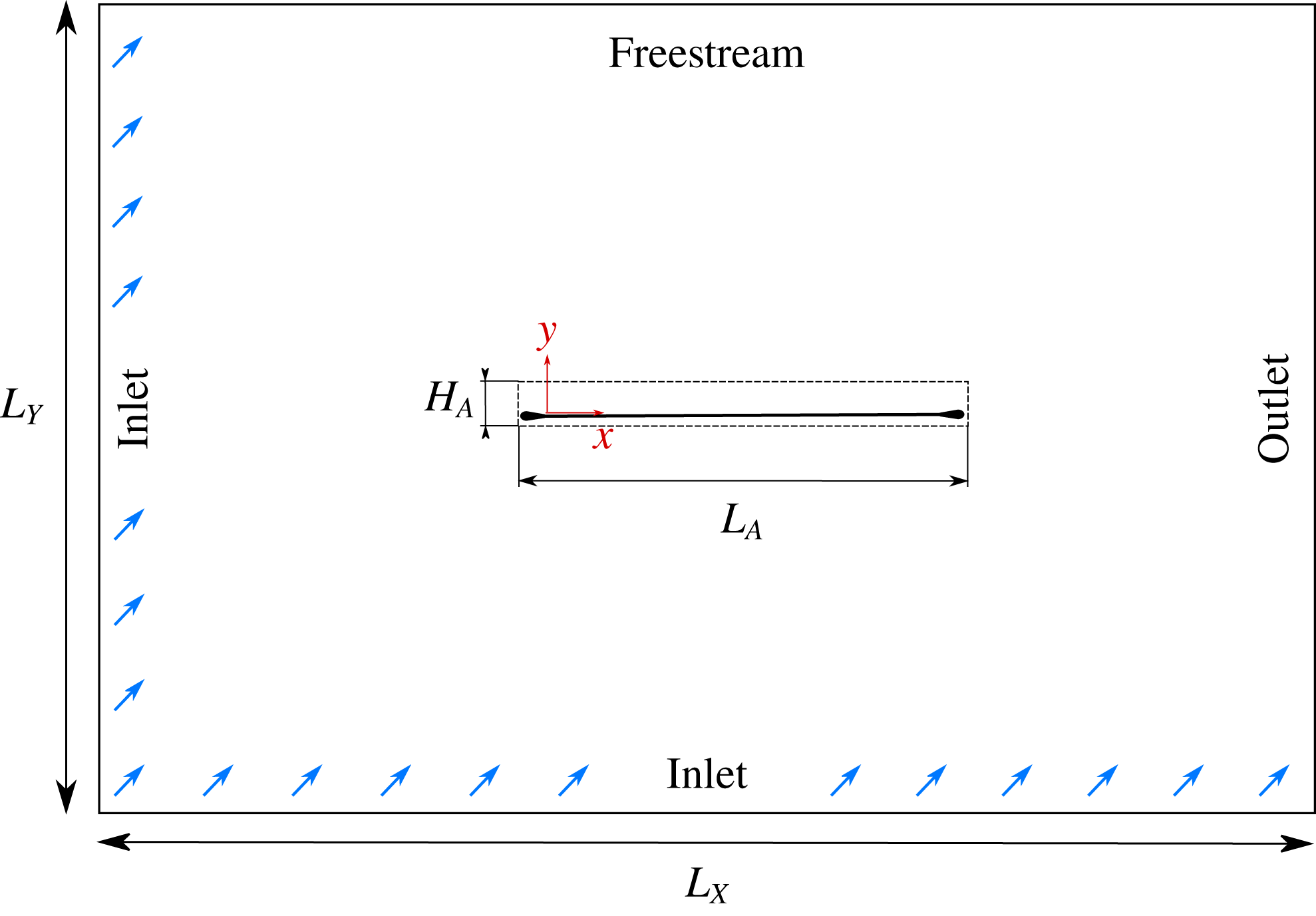
The discretised fluid equations are solved in an Eulerian Cartesian grid of dimensions
 $L_{X}=61$
by
 $L_{Y}=60.1$
, with a refined central area where the membrane is located, as shown in figure 1. The lower and left boundaries are treated as inlets and an integral characteristic boundary condition for a uniform unity velocity deflected by 8 degrees is applied. At the free-stream upper boundary a non-reflecting characteristic boundary condition was used and at the right outlet edge a zonal characteristic boundary condition is applied (Sandberg & Sandham Reference Sandberg and Sandham2006). At the aerofoil surface the non-slip isothermal boundary condition is applied via an immersed boundary technique described in § 2.3. The number of in-plane computational grid points used for the flow solver was
 $(N_{x},N_{y})=(1103\,783)$
. The length of the fine-grid region,
 $L_{A}$
, is set to the chord length (
 $L_{m}$
) plus the length of the supports and the height is
 $H_{A}=0.1$
, covering the maximum height expected for the deflected membrane. In this finer area the points are distributed equidistantly in the wall-normal direction with resolution
 $\unicode[STIX]{x0394}y=2.5\times 10^{-4}$
, estimated to include at least six Eulerian grid points over the membrane thickness to ensure accuracy of the interpolation between fluid and structure grids. In the streamwise direction the grid is stretched towards the midpoint of the membrane, with a minimum spacing around the leading and trailing edges of
 $\unicode[STIX]{x0394}x=5\times 10^{-4}$
, which assures a minimum ratio of
 $1:4$
Langrangian to Eulerian points necessary for interpolation. The distribution of points away from this region is stretched towards the boundaries of the domain by means of a fifth-order polynomial function. The grid resolution and domain size were established by an iterative process until the results were proven to be grid-independent (see details in Serrano-Galiano & Sandberg Reference Serrano-Galiano and Sandberg2015). The suitability of the grid resolution is also confirmed by a posteriori calculation of the wall units with the statistical data from the 3D simulation. With the resolution in the streamwise and the wall-normal direction specified above, the corresponding resolution in wall units at the location of maximum mean skin friction coefficient (
 $\overline{C_{f}}=0.017$
at
 $x=0.573$
, data given in § 6.2, figure 18
c) are
 $\unicode[STIX]{x0394}x^{+}=3.80$
and
 $\unicode[STIX]{x0394}y^{+}=0.23$
. These values are comparable to those of the DNS simulation of a turbulent flow around an aerofoil from Jones, Sandberg & Sandham (Reference Jones, Sandberg and Sandham2008). The suitability of the spanwise domain size will be further discussed in the context of two-point correlations in § 6 of this paper.
Sketch of the computational domain. The dashed line rectangle delimits the Eulerian fine-grid region. Blue arrows at the inlet boundaries symbolise the incoming flow deflected 8 degrees with respect to the horizontal (
 $x$
) axis.

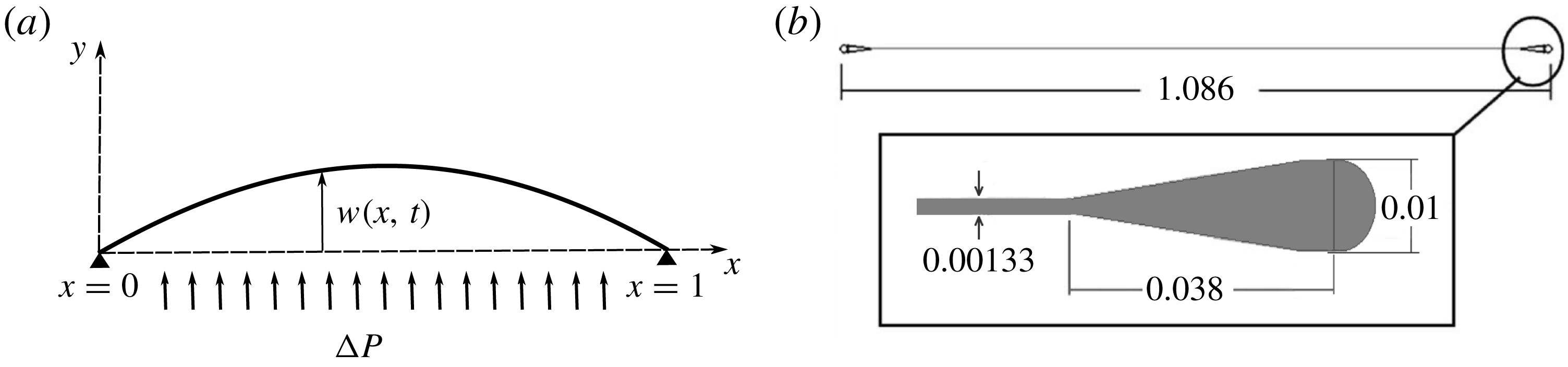
(a) Sketch of the membrane configuration, pinned at both ends. (b) Sketch of the membrane aerofoil with aerodynamic shaped mounts based on the set-up from Rojratsirikul et al. (Reference Rojratsirikul, Wang and Gursul2009). The length of the undisturbed elastic sheet is taken as the reference length.

2.2 Structural solver
The aerofoil configuration simulated here is based on the model from Rojratsirikul et al. (Reference Rojratsirikul, Wang and Gursul2009), composed of a latex sheet mounted onto two rigid aerodynamically shaped mounts at the leading and trailing edges. The characteristic length used for non-dimensionalisation of the problem is the actual length of the latex sheet, resulting in a total chord length of the aerofoil, including mounts, of
 $1.086$
non-dimensional units. The membrane length,
 $L_{m}$
is then one non-dimensional unit and the non-dimensional thickness is chosen as
 $h=1.33\times 10^{-3}$
.
The membrane is considered as a one-dimensional continuum solid having larger length than thickness, whose restoring forces arise from the in-plane tensile forces. The membrane is assumed to have no resistance to shear and bending, to have a straight line equilibrium configuration and to be subject to pressure forces normal to its surface. The membrane is fixed at both ends as shown in figure 2. The governing equation is obtained from the balance of forces applied to an element of elastic string and applying the condition of fixed ends as proposed in Carrier (Reference Carrier1945). In particular, the formulation of the structural model for the membrane used in this study is based on that from Gordnier (Reference Gordnier2009). The equation in non-dimensional form for the vertical dimensionless deflection
 $w(x,t)$
in this case is
 $$\begin{eqnarray}\unicode[STIX]{x1D70C}_{s}h\frac{\unicode[STIX]{x2202}^{2}w}{\unicode[STIX]{x2202}t^{2}}-T_{s}\frac{\unicode[STIX]{x2202}^{2}w}{\unicode[STIX]{x2202}x^{2}}\left[1+\left(\frac{\unicode[STIX]{x2202}w}{\unicode[STIX]{x2202}x}\right)^{2}\right]^{-3/2}=\unicode[STIX]{x0394}p,\end{eqnarray}$$
with the boundary conditions
 $w(x=0,t)=0$
and
 $w(x=1,t)=0$
. The membrane material is assumed to be linearly elastic and the membrane tension
 $T_{s}$
can be written in terms of the membrane strain
 $\unicode[STIX]{x1D6FF}_{s}$
and prestrain
 $\unicode[STIX]{x1D6FF}_{s0}$
as
 $$\begin{eqnarray}T_{s}=E_{s}h\left(\unicode[STIX]{x1D6FF}_{s0}+\unicode[STIX]{x1D6FF}_{s}\right),\quad \text{where }\unicode[STIX]{x1D6FF}_{s}=L-1,\;L=\int _{0}^{1}\sqrt{1+\left(\frac{\unicode[STIX]{x2202}w}{\unicode[STIX]{x2202}x}\right)^{2}}\,\text{d}x.\end{eqnarray}$$
In the 3D simulations the membrane is extruded in the spanwise direction, not allowing spanwise deformations, i.e. assuming a material with infinite stiffness in the
 $z$
-direction. The membrane material density,
 $\unicode[STIX]{x1D70C}_{s}$
, and modulus of elasticity,
 $E_{s}$
, as well as the membrane thickness,
 $h$
, are assumed to be constant and uniform along the longitudinal (
 $x$
) direction. The pressure force term
 $\unicode[STIX]{x0394}p$
is defined as the difference of pressure between the upper and lower surface of the membrane immersed in the flow. This term is responsible for coupling the flow behaviour and the membrane response. The structural equation and structural variables were non-dimensionalised with the flow free-stream velocity and density and the membrane length. The resulting dimensionless structural parameters are
 $\unicode[STIX]{x1D70C}_{s}h$
,
 $E_{s}h$
,
 $\unicode[STIX]{x1D6FF}_{s0}$
. For the simulations carried out for this work these non-dimensional parameters were set as
 $\unicode[STIX]{x1D70C}_{s}h=0.583$
,
 $E_{s}h=50$
and
 $\unicode[STIX]{x1D6FF}_{s0}=0$
, based on previous experimental (Rojratsirikul et al.
Reference Rojratsirikul, Wang and Gursul2009) and computational (Gordnier Reference Gordnier2009) studies.
In the structural solver the governing equation (2.1), involving a second derivative in time, is rewritten as a system of two equations with only first derivatives in time. The first and second spatial derivatives are evaluated by means of a fourth-order accurate compact finite difference scheme. The resulting system of equations discretised in space is advanced in time using the same fourth-order Runge–Kutta method as used for the flow. The boundary conditions impose zero displacement and velocity for the first and last point of the membrane, attached to the rigid leading and trailing edge respectively. The one-dimensional Lagrangian grid for the structural solver includes 100 equispaced points along the membrane length, which allows the membrane dynamic response to be resolved with a minimum wavelength of 2 % of the chord.
2.3 Fluid–structure coupling
In the coupled fluid–structure computational set-up the fluid solver is used to determine the state variables of the flow around a membrane aerofoil, in particular the flow velocity and difference of pressure between the lower and upper surfaces. Once the difference of pressure is known, it is introduced as
 $\unicode[STIX]{x0394}p$
in the one-dimensional structural equation (2.1) that is solved to determine the displacement,
 $w$
, and lateral velocity of the membrane. The new position of the mid-line of the membrane with respect to its original location is
 $w$
and the new shape of the aerofoil is then recomputed around it by adding the corresponding constant semithickness. Once the deformed geometry is determined it is imposed as a non-slip boundary condition into the flow field and the process starts again calculating the new
 $\unicode[STIX]{x0394}p$
and the new deflection that it induces, and so on for each new time step of the simulation. Some previous studies solved the fluid and structure equations separately and then coupled them through a subiteration process (Smith & Shyy Reference Smith and Shyy1997; Lian et al.
Reference Lian, Shyy, Ifju and Verron2002; Gordnier Reference Gordnier2009). The approach used here is to solve both systems of partial differential equations simultaneously each time step with information exchanged between them at the end of each full time step of the simulation. Based on Courant number requirements for stability of explicit time advancement methods, the time step used for the direct numerical simulations is between one and two orders of magnitude smaller than the time step required for the structure (Serrano-Galiano Reference Serrano-Galiano2016). Therefore the time lag between the pressure term and structural deflection is negligible and no subiterations are needed.
The method applied here to impose the geometry and boundary conditions of the solid body immersed in the flow is the boundary data immersion method (BDIM) of Weymouth & Yue (Reference Weymouth and Yue2011) adapted for compressible flows by Schlanderer, Weymouth & Sandberg (Reference Schlanderer, Weymouth and Sandberg2017). This immersed boundary formulation combines the governing equations from the fluid and solid domains and the interface conditions analytically, resulting in a set of meta-equations valid in the full domain. The resulting equations from the BDIM are applied after the numerical time integration and no modifications of the individual solver algorithms are needed. The validity of this method to accurately simulate the hydrodynamic and acoustic field around immersed steady and moving bodies has been shown in Schlanderer & Sandberg (Reference Schlanderer and Sandberg2014) and Schlanderer et al. (Reference Schlanderer, Weymouth and Sandberg2017). Validations of the coupled fluid–structure computational set-up for simulating a membrane aerofoil in steady and unsteady conditions and comparison of results with reference studies can be found in Serrano-Galiano & Sandberg (Reference Serrano-Galiano and Sandberg2015) and Serrano-Galiano (Reference Serrano-Galiano2016). Grid-dependence studies can also be found in the last reference, showing no variation of lift coefficient and mean deflection and variation of only
 $0.08\,\%$
in pressure coefficient for a grid refined by
 $36.6\,\%$
in the wall-normal direction.
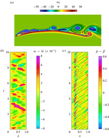
(a) Instantaneous spanwise vorticity field (
 $\unicode[STIX]{x1D714}_{z}$
). (b,c)
 $x$
-
 $t$
-diagrams of fluctuations of the membrane deflection (
 $w-\overline{w}$
) (b) and the pressure on the upper surface (
 $p-\overline{p}$
) (c).

3 Dynamics of membrane aerofoils
We begin the analysis by considering purely 2D cases. The static effect of the pressure distribution around the membrane aerofoil is the mean camber induced in the membrane. The mean pressure distribution is characterised by a laminar separation bubble with reattachment and later separation of the boundary layer in the aft section of the aerofoil. Additionally, fluctuations in pressure cause fluctuations of the membrane around its mean position and vice versa. The content of the following sections focuses on the analysis of the pressure and deflection fluctuations and the relation between them; details about the system mean behaviour can be found in Serrano-Galiano (Reference Serrano-Galiano2016).
The instantaneous pressure field around the aerofoil is characterised by vortices shed from the leading edge (LE) recirculation region that are convected over the upper surface of the membrane, as can be observed in the instantaneous spanwise vorticity fields in figure 3(a). The vortices cause regions of instantaneous low pressure simultaneously at various locations along the chord, coinciding with the streamwise location of the vortices. Figure 3(c) illustrates the time history of the upper surface pressure fluctuations,
 $p-\overline{p}$
, along the chord for a time interval of ten non-dimensional time units, where the influence of the different vortex shedding characteristics can be seen. The vortex shedding is not completely regular and shows different time scales, corresponding to different phenomena such as detached vortices that stay close to the surface, vortices that are lifted further from the surface, vortices convecting with different speeds, and occasional vortex merging near the trailing edge (TE). A dominant pattern of downstream-travelling pressure waves is observed as diagonal stripes of low pressure values. Additionally, some pressure fluctuations travelling from the trailing to the leading edge are observed with a lower frequency. Pressure differences between the upper and lower surfaces (i.e. the forcing term of the membrane equation) are almost entirely due to upper surface pressure fluctuations since the pressure on the lower surface does not show significant variation along the chord. For this reason, from now on, the investigation on pressure dynamics will focus only on the upper surface pressure behaviour.
The fluctuations around the mean displacement for the membrane are plotted along the chord in the
 $x$
-
 $t$
-diagrams in figure 3(b). The membrane fluctuations are dominated by downstream- and upstream-travelling waves. Despite the underlying combination of vibration modes, standing waves are visible at some points in time, sometimes close to a third and sometimes close to a second mode.
The pressure fluctuations act as an excitation source that drives the membrane movement. To get a deeper understanding of the membrane behaviour it is useful to think briefly about the solution of the homogeneous linearised model equation of a one-dimensional membrane with both ends fixed. The general solution of the free vibration problem can be written as a superposition of all particular solutions as (see Graff (Reference Graff1975) for the full mathematical development)
 $$\begin{eqnarray}\displaystyle w(x,t) & = & \displaystyle \mathop{\sum }_{n=1}^{\infty }A_{n}\cos (\unicode[STIX]{x1D705}_{n}x-{\unicode[STIX]{x1D714}_{r}}_{n}t)-A_{n}\cos (\unicode[STIX]{x1D705}_{n}x+{\unicode[STIX]{x1D714}_{r}}_{n}t)\nonumber\\ \displaystyle & & \displaystyle +\,B_{n}\sin (\unicode[STIX]{x1D705}_{n}x+{\unicode[STIX]{x1D714}_{r}}_{n}t)+B_{n}\sin (\unicode[STIX]{x1D705}_{n}x-{\unicode[STIX]{x1D714}_{r}}_{n}t)\nonumber\\ \displaystyle & = & \displaystyle \mathop{\sum }_{n=1}^{\infty }(2A_{n}\sin ({\unicode[STIX]{x1D714}_{r}}_{n}t)+2B_{n}\cos ({\unicode[STIX]{x1D714}_{r}}_{n}t))\sin (\unicode[STIX]{x1D705}_{n}x).\end{eqnarray}$$
The first part of this equality shows that the motion of the system is governed by propagating waves in the positive (argument (
 $\unicode[STIX]{x1D705}_{n}x-{\unicode[STIX]{x1D714}_{r}}_{n}t$
)) and negative
 $x$
-direction (argument (
 $\unicode[STIX]{x1D705}_{n}x+{\unicode[STIX]{x1D714}_{r}}_{n}t$
)) with wavenumber
 $\unicode[STIX]{x1D705}_{n}=2\unicode[STIX]{x03C0}/\unicode[STIX]{x1D706}_{n}$
, radial frequency
 ${\unicode[STIX]{x1D714}_{r}}_{n}=2\unicode[STIX]{x03C0}f_{n}$
, wavelength
 $\unicode[STIX]{x1D706}_{n}$
and frequency
 $f_{n}$
. When the boundary condition of both ends being fixed is imposed the wavenumber and frequency of each particular solution must fulfil the relation
 $$\begin{eqnarray}{\unicode[STIX]{x1D714}_{r}}_{n}=c_{ph}\unicode[STIX]{x1D705}_{n},\quad c_{ph}=\sqrt{T_{s}/(\unicode[STIX]{x1D70C}_{s}h)}.\end{eqnarray}$$
The second part of the equality represents a pure standing wave pattern, where the spatial and temporal variations of the membrane displacement are independent, and with points of maximum and zero amplitude fixed in space for each value of
 $n$
. The natural frequencies of the linear system are denoted
 ${\unicode[STIX]{x1D714}_{r}}_{n}$
and the corresponding normal modes take the form of
 $\sin (\unicode[STIX]{x1D705}_{n}x)$
. The existence of such waves can only occur due to the interaction of two waves of the same type, amplitude and frequency, travelling in opposite directions with phase velocity
 $c_{ph}$
and the appropriate phase difference.
When the elastic membrane moves under an external forcing and nonlinearity is taken into account, the movement of the system will be the result of a more complex interference of the enforced travelling waves and their reflections from the boundaries, unless the forcing frequency coincides with some of the natural frequencies of the system, causing some resonance reinforcing specific modes. Natural frequencies for the membrane are included in Serrano-Galiano (Reference Serrano-Galiano2016), where it is shown how the lowest domain frequencies lie in between the first two natural frequencies computed with and without an added mass correction. At higher frequencies the differences between the observed and predicted frequencies are larger. Despite the additional complexity of the membrane vibration not strictly following the normal mode solution (3.1), in our case the wave nature of the solution is still maintained. Therefore Fourier transformation for the analysis in the frequency and wavenumber space is carried out in the following sections as a way to break down the flow–structure coupled problem in the search for further understanding.
3.1 Wavenumber–frequency spectrum
A double Fourier transform was applied to the discrete pressure and deflection signals in time and space, to map the functions into both frequency and wavenumber space through the mathematical expression
 $$\begin{eqnarray}{\mathcal{F}}(p(x,t))(\unicode[STIX]{x1D706},f)=\frac{1}{N}\frac{1}{M}\mathop{\sum }_{t=0}^{N-1}\mathop{\sum }_{x=0}^{M-1}p(x,t)\text{e}^{-\text{i}2\unicode[STIX]{x03C0}ft}\text{e}^{-\text{i}(2\unicode[STIX]{x03C0}/\unicode[STIX]{x1D706})x}.\end{eqnarray}$$
To compute the wavenumber–frequency spectra the data along a line over the aerofoil surface was extracted and stored as a time–space matrix containing physical values at 100
 $x$
-locations along the chord and for 318 non-dimensional time units (60 000 equispaced data samples) divided into 14 segments for averaging. Then a Fourier transform in time was applied to the time signal at each point using segmentation and Hanning windowing, and, for each frequency, the signal along the points in the aerofoil surface was complex-Fourier-transformed in space, also with windowing but with no segmentation due to the shorter length of the signal in space. The results of the double transformation are shown in figure 4 as 2D plots that depict the amplitude as a function of the non-dimensional frequency, or Strouhal number (
 $St=fL_{m}/u_{\infty }=\unicode[STIX]{x1D714}_{r}/2\unicode[STIX]{x03C0}$
), on the
 $y$
-axis and the inverse of the non-dimensional wavelength (
 $1/\unicode[STIX]{x1D706}=\unicode[STIX]{x1D705}/2\unicode[STIX]{x03C0}$
) on the
 $x$
-axis, similarly to the wavenumber–frequency diagrams introduced by Bremner & Wilby (Reference Bremner and Wilby2002). Note that when the wavenumber is mentioned in this section, it should be taken as
 $\unicode[STIX]{x1D705}/2\unicode[STIX]{x03C0}$
. It must also be pointed out that in figure 4 positive wavenumbers and positive frequencies indicate downstream-propagating waves, and the negative wavenumber sector contains the upstream-propagating waves; i.e. for a more intuitive perception, the original spectrum containing positive and negative frequencies and wavenumbers, consistent with the formulation in expression (3.1), is mirrored with respect to the
 $St=0$
axis and just the positive frequency sector is plotted, which contains all the information. Lines with constant slope can then be interpreted as constant phase velocity lines, with
 $c_{ph}=f/(1/\unicode[STIX]{x1D706})=f\unicode[STIX]{x1D706}$
.
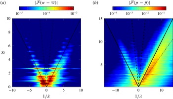
Wavenumber–frequency spectra of (a) membrane fluctuations around its mean position (
 $w$
), and (b) pressure (
 $p$
) fluctuations along the upper surface of the membrane. Lines corresponding to free-stream propagation velocity (——),
 $70\,\%$
of the free-stream propagation velocity (
 $\cdots \cdots$
) and sound propagation velocity (- -) are included as reference.

Figure 4(a) shows two almost symmetric branches in the wavenumber–frequency spectrum of the membrane oscillations, which indicates a similar amount of waves travelling upstream and downstream through the membrane, corresponding to the motion induced by the flow and the reflections of the waves from the supports. The highest-amplitude peaks are almost aligned with a line indicating a phase speed of approximately one (the solid black line in the plot), i.e. equal to the free-stream velocity. The highest concentration of energy appears at frequencies below 2, particularly for
 $St\approx 0.53$
and
 $0.9$
, corresponding to the first and second structural modes. The amplitudes of the coefficients decay as the frequency increases. An indication of a third mode can be distinguished at
 $St\approx 1.56$
and also a low-amplitude fifth mode seems to appear at
 $St\approx 2.7$
. The corresponding wavenumbers to these amplitude peaks coincide approximately with the wavenumbers expected for the normal modes of the linear model. Only when the peaks of positive and negative wavenumber for a given frequency are perfectly symmetric would there be a standing wave pattern.
In the wavenumber–frequency spectrum of pressure fluctuations (figure 4
b) the symmetry between branches corresponding to upstream- and downstream-propagating waves is lost. The downstream branch is larger and wider, corresponding to a broader range of pressure waves for the different time and space scales present in the flow. This branch shows a slope of approximately
 $0.8$
, which indicates a phase speed of approximately
 $0.8u_{\infty }$
, corresponding to the convection speed expected for hydrodynamic pressure fluctuations. The most energetic frequency is found to be
 $St\approx 2.7$
. Significant energy content is also found for
 $St\approx 1.56$
and
 $1.3$
. Additionally, the frequency that seems to indicate a second structural mode,
 $St\approx 0.9$
, is a dominant frequency in the surface pressure spectrum. The upstream branch is limited to lower frequencies and wavenumbers, showing discrete peaks almost symmetric to those on the upstream branch at approximately the same frequencies as in the deflection fluctuations. The slope of the upstream branch is approximately
 $-1$
, which would correspond to
 $c_{ph}\approx -u_{\infty }$
. It is unusual to find pressure fluctuations travelling upstream with a phase speed in the hydrodynamic range; they would rather be expected to propagate with a phase speed in the acoustic waves range, marked with black dashed lines in the plot. In fact, a small upstream branch with lower amplitude corresponding to pressure waves travelling upstream with phase speed aligned with the acoustic wave propagation speed (dashed lines in the plot) can also be distinguished.
These results suggest that the membrane redistributes the energy into specific frequencies of the coupled system. It is excited by the flow pressure fluctuations over a wide range of frequencies, but it responds by transferring this vibration energy into just a few discrete low frequencies. The clear presence of unexpected ‘slow’ upstream-travelling pressure waves on the upper surface of the aerofoil can most likely be attributed to the fluid–structure interaction, and this will be investigated in detail in the next sections.
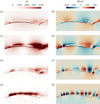
Contours of the amplitude (a,c,e,g) and real part (b,d,f,h) of the Fourier transform coefficients of the pressure field corresponding to the non-dimensional frequency (a,b)
 $St=0.52$
, (c,d)
 $St=0.9$
, (e,f)
 $St=1.56$
and (g,h)
 $St=2.7$
.

3.2 Fourier-transformed pressure field
To get a deeper insight into the flow phenomena that occur periodically at the dominant frequencies observed in § 3.1, the full pressure field was Fourier-transformed in time. This gives an overview of the pressure fluctuations around the aerofoil, not only limited to the surface. The amplitude (computed as the square root of the product of the complex pressure modes with their complex conjugates) and the real part of the Fourier-transformed pressure is shown in figure 5 for four of the dominant frequencies found in the pressure and deflection spectra, i.e.
 $St=0.52,0.9,1.56$
and
 $2.7$
. In this case the time signals used for the Fourier transformation were reduced in length compared to those used for the spectra on the surface, as the range of frequencies of interest is smaller. The pressure time signals corresponding to
 $21.2$
time units (1600 equispaced data samples) were divided into three segments for averaging.
Figure 5(a,b) corresponds to the dimensionless frequency
 $St=0.52$
, which is the frequency of the membrane first mode of oscillation. In this figure, the amplitude of the Fourier-transformed pressure shows high values close to the membrane surface. This indicates that the membrane movement induces long-period pressure fluctuations mainly close to the surface, and the pressure waves in the streamwise direction seem to have a wavelength of approximately one chord, as indicated by the contours of the real part of the Fourier coefficients.
At
 $St=0.9$
, high amplitude is observed at two locations in the Fourier-transformed pressure field in figure 5(c,d). The two locations where the high amplitudes appear correspond to the locations where vortices detach from the recirculation bubble and to the location of separation and vortex merging in the proximity of the trailing edge. Therefore, the phenomena observed at this frequency seem to correspond to a coupling between the membrane second mode of vibration and the shedding of faster vortices from the LE, combined with vortex slowdown and merging around the TE.
At
 $St=1.56$
the highest amplitude is observed in the wake, but very close to the TE (see figure 5
e,f). This is also the frequency that shows the highest energy content in the spectrum computed for a monitor point in the wake. There are no significant levels near the membrane surface, except at the location of reattachment. Also the real part of the Fourier coefficients seems to indicate that the pressure waves emerge in the vicinity of the TE, therefore the phenomena at this frequency seem to be related to the wake shedding.
Contours of the amplitude of the Fourier coefficients at
 $St=2.7$
, the dominant frequency for the vortex shedding from the leading edge, are shown in figure 5(g,h). The real part has the form of pressure waves originating from near the location of the reattachment point for the mean flow separation bubble, which is the origin of the shed vortices. This pattern also indicates a smaller wavelength compared to the previous frequencies. High amplitudes of the Fourier transform of the pressure can be seen approximately along the centre of the external shear layer over the aerofoil.
In summary, the real part of the Fourier coefficients from the Fourier transform of the pressure field shows smaller spatial scales of the pressure fluctuations as the frequency increases, and it seems that the higher frequencies are associated with flow-induced movement, while the membrane movement is related to lower-frequency oscillations.
 $x$
-
 $t$
-diagrams of the full pressure fluctuations (
 $p-\overline{p}$
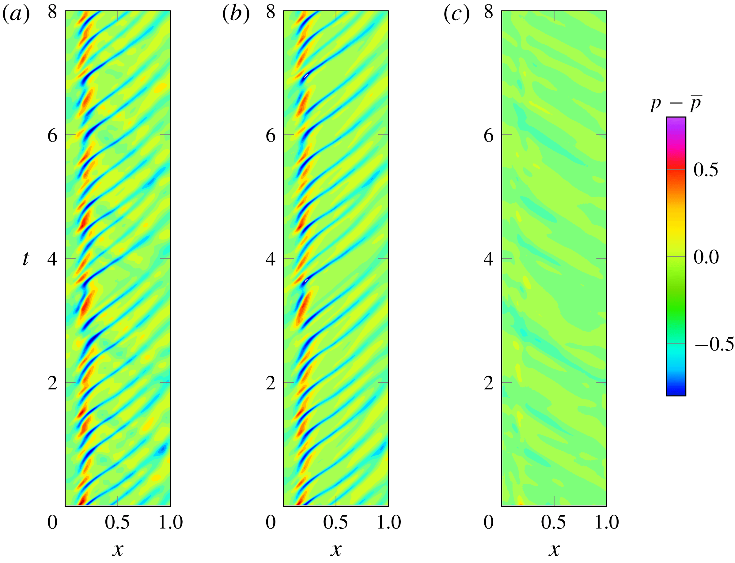
) on the upper surface of the membrane (a), and decomposed into downstream (b) and upstream (c) pressure waves components.

4 Fluid–structure coupling mechanism for membrane aerofoils
4.1 Separation of upstream- and downstream-travelling pressure waves
As seen in § 3.1, once the data of the time evolution of the pressure fluctuations along the chord is transformed to the wavenumber–frequency space, a differentiation between upstream- and downstream-travelling waves is possible according to the signs of
 $St$
and
 $1/\unicode[STIX]{x1D706}$
. In this section the data in wavenumber–frequency space is filtered according to the propagation direction and the inverse of the double Fourier transform is performed to analyse the filtered data back in physical space. The data used contain the time history of the upper surface pressure fluctuations and are just a part of the data used in § 3.1, corresponding to the last 53 time units. No segmentation, averaging or windowing was used in this case for the direct and inverse Fourier transforms. The
 $x$
-
 $t$
-diagrams in figure 6 illustrate the original data set and the results from the filtering.
When the upstream-propagating part of the signal is suppressed, we basically observe the footprint of the vortices convecting downstream over the surface in the form of low-pressure stripes, as described in § 3 as a dominant feature of the surface pressure. On the other hand, when the downstream part is suppressed, the presence of upstream-travelling waves is revealed. This is the most interesting part of the decomposition, and its corresponding diagram (figure 6
c) shows low-pressure waves propagating from the TE to the LE in a periodic manner with a slope of approximately
 $-1$
. Once the data were decomposed, each part of the pressure was correlated with the membrane deflection to further understand the coupling between pressure and membrane oscillations.
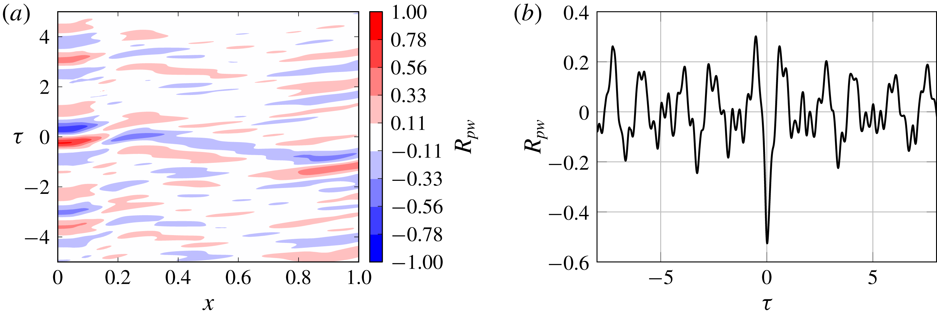
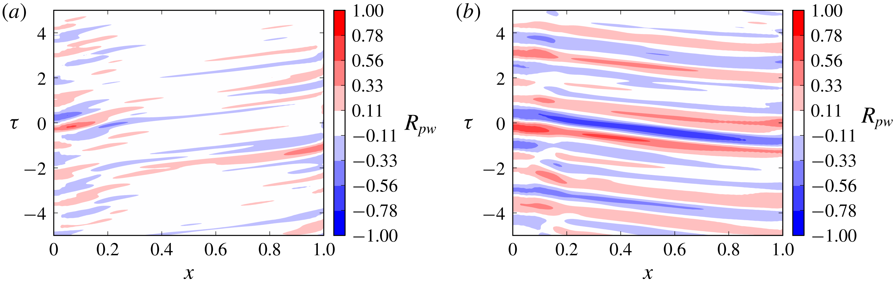
(a) Contours of cross-correlation between the time signal of deflection fluctuations at location
 $x=0.27$
and the time signals of pressure fluctuations along the membrane upper surface. (b) Cross-correlation between pressure and deflection fluctuations at the location of maximum
 $w_{rms}$
,
 $x=0.27$
.

4.2 Correlation between deflection and full pressure signals
The correlations presented here are calculated by dividing the pressure and deflection signals into four segments and averaging the individual segment correlations. The values of the correlation over each non-dimensional time shift
 $\unicode[STIX]{x1D70F}$
are normalised with the root mean square (r.m.s.) value of the time signal.
Cross-correlations between pressure and deflection time signals have been computed at a fixed location for the deflection signal (the location of the maximum r.m.s. deflection), and at all the 100 points along the chord for the pressure signal with the aim of identifying whether there are specific locations with a stronger relationship between the two variables. The result is shown in a 2D plot on figure 7(a) using ten contour levels to express the normalised cross-correlation coefficient value against location (
 $x$
) and time shift (
 $\unicode[STIX]{x1D70F}$
). The largest values of correlation are seen in the first and last
 $25\,\%$
of the chord. Most importantly, some inclined stripes of positive and negative correlation values indicate that the strongest correlation between pressure and deflection does not occur at a fixed chordwise location but follows the upstream and downstream wave propagation. This will be clarified later by investigating the correlation between the deflection and the upstream- or downstream-travelling pressure components. A shift in the correlation sign is observed around
 $x=0.18$
that can be attributed to the strong pressure gradient through the recirculation bubble and reattachment. Figure 7(b) shows a slice through the contour plot at
 $x=0.27$
, which represents the cross-correlation between pressure and deflection at the location of maximum deflection r.m.s. The negative value of correlation found at
 $\unicode[STIX]{x1D70F}=0$
indicates that, at the same point and at the same time, pressure and deflection tend to have opposite sign, i.e. instantaneous positive pressure fluctuations (pressure value above the mean) cause instantaneous negative deflection fluctuations (deflection value below the mean) and vice versa. Some kind of periodicity is also observed in figure 7(b), although it is difficult to draw further conclusions as there are different time scales involved.
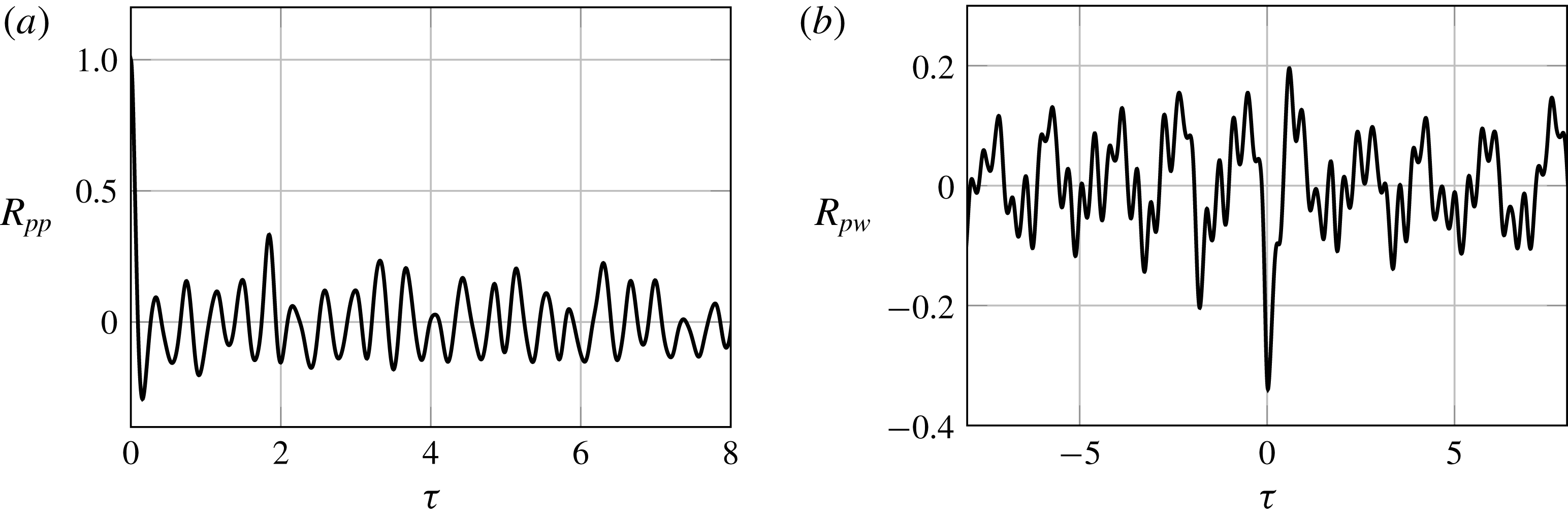
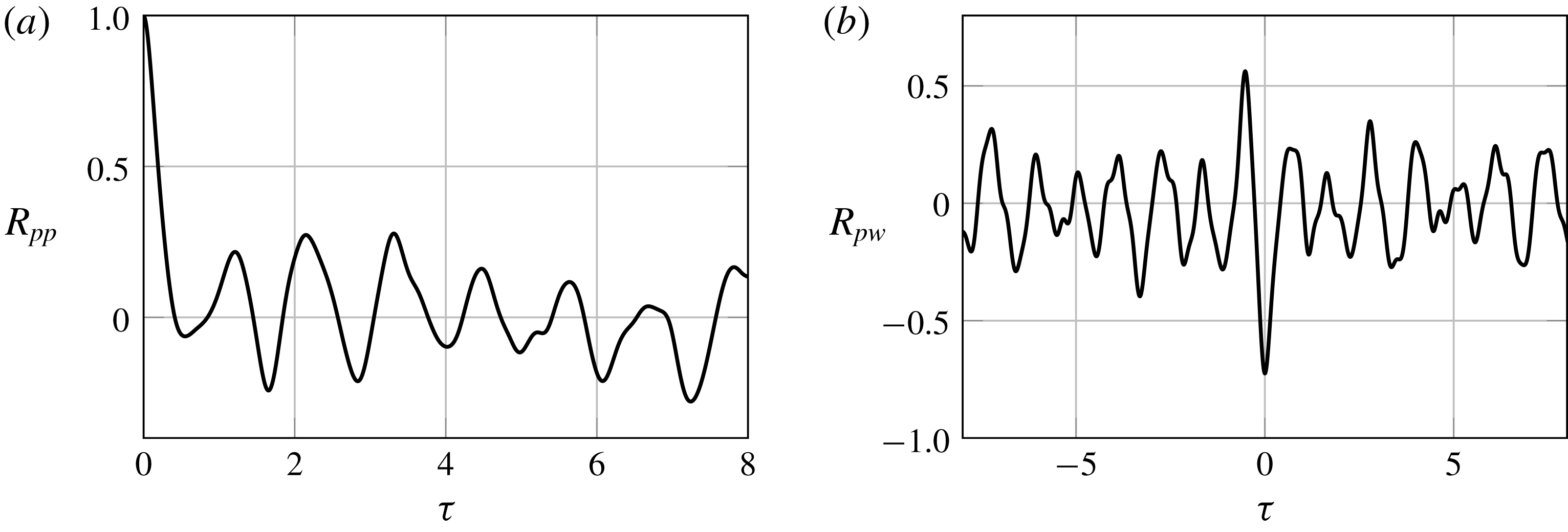
(a) Autocorrelation of pressure fluctuation at the upper surface location of maximum
 $p_{rms}$
,
 $x=0.20$
. (b) Cross-correlation of membrane fluctuation and upper surface pressure at the membrane location of maximum
 $w_{rms}$
,
 $x=0.27$
. For both plots, the upper surface pressure time signal was filtered to contain only the downstream-travelling component.

(a) Contours of cross-correlation between the time signal of deflection fluctuations at location
 $x=0.27$
and the filtered time signals of pressure fluctuations travelling downstream along the membrane upper surface. (b) Contours of cross-correlation between the time signal of deflection fluctuations at location
 $x=0.27$
and the filtered time signals of pressure fluctuations travelling upstream along the membrane upper surface.

4.3 Correlation between deflection and downstream and upstream pressure signals
The same type of correlations were computed for the components of pressure obtained after the filter operation was performed in wavenumber–frequency space, as explained in § 4.1. The autocorrelation of the downstream-travelling pressure waves at the location of maximum pressure r.m.s. value,
 $x=0.2$
, is shown in figure 8(a). The periodicity of the signal is very clear. The peaks in the autocorrelation appear approximately in equispaced intervals of
 $\unicode[STIX]{x1D70F}\approx 0.35$
corresponding to the frequency
 $St\approx 2.7$
found in the frequency spectrum (figure 4
b). This, together with the time-evolution pattern observed in the
 $x$
-
 $t$
-diagram corresponding to only the downstream-travelling pressure waves, confirms what was stated in § 3.2: the dominant frequency
 $St=2.7$
corresponds to the vortices shed from the LE recirculation bubble.
(a) Autocorrelation of pressure fluctuation at the upper surface location of maximum
 $p_{rms}$
,
 $x=0.20$
. (b) Cross-correlation of membrane fluctuation and upper surface pressure at the membrane location of maximum
 $w_{rms}$
,
 $x=0.27$
. For both plots, the upper surface pressure time signal was filtered to contain only the upstream-travelling component.

The cross-correlation between the downstream pressure component along the chord and the membrane deflection at
 $x=0.27$
is depicted in figure 9(a). Moderately high values of correlation are observed only over the first
 $25\,\%$
and the last
 $10\,\%$
of the chord, which seem to indicate that the fluctuations are to a certain extent linearly related at the location of the strongest pressure variation due to the vortex shedding. After a time
 $\unicode[STIX]{x1D70F}\approx 1.3$
(in agreement with a convection speed of
 $C_{ph}\approx 0.75$
) this relation seems to be observed again at the TE where strong pressure fluctuations also occur, due to separation. In between, pressure and deflection appear to be very weakly correlated. This can be explained due to the difference in time scale of the membrane, with slower long-wavelength fluctuations, and pressure, with faster short-wavelength vortex-induced fluctuations. A different situation is found when the upstream-propagating component of the pressure waves is considered. The autocorrelation of upstream-travelling pressure waves at the location of maximum pressure r.m.s. in figure 10(a) shows periodicity with larger periods of
 $\unicode[STIX]{x1D70F}\approx 1.1$
. This period coincides with one of the relevant frequencies,
 $St\approx 0.9$
, found in the wavenumber–frequency spectrum of the deflection time signal (figure 4
b). When the cross-correlation between upstream pressure and deflection is computed (figure 9
b), the relation between membrane deflection and upstream pressure waves can be clearly appreciated. Inclined stripes of
 $R_{pw}\approx \pm 0.5$
extending along the full chord with a negative slope of approximately
 $-1.15$
indicate that the relation between pressure and deflection is maintained as the distance along the chord is travelled at a speed
 $c_{ph}\approx 0.87$
from the TE to the LE, i.e. if a positive correlation is found at
 $t=0$
at the TE, this positive correlation will be found
 $\unicode[STIX]{x1D70F}\approx 1.15$
later at the LE, maintaining the same level of correlation all the way through. This value of phase speed corresponds approximately to the phase speed of second mode waves with
 $St\approx 0.9$
propagating through the membrane, identified as one of the most energetic frequencies of the membrane vibration in the spectrum (
 $c_{ph}=f/(1/\unicode[STIX]{x1D706})\approx 0.9L_{m}=0.9$
).
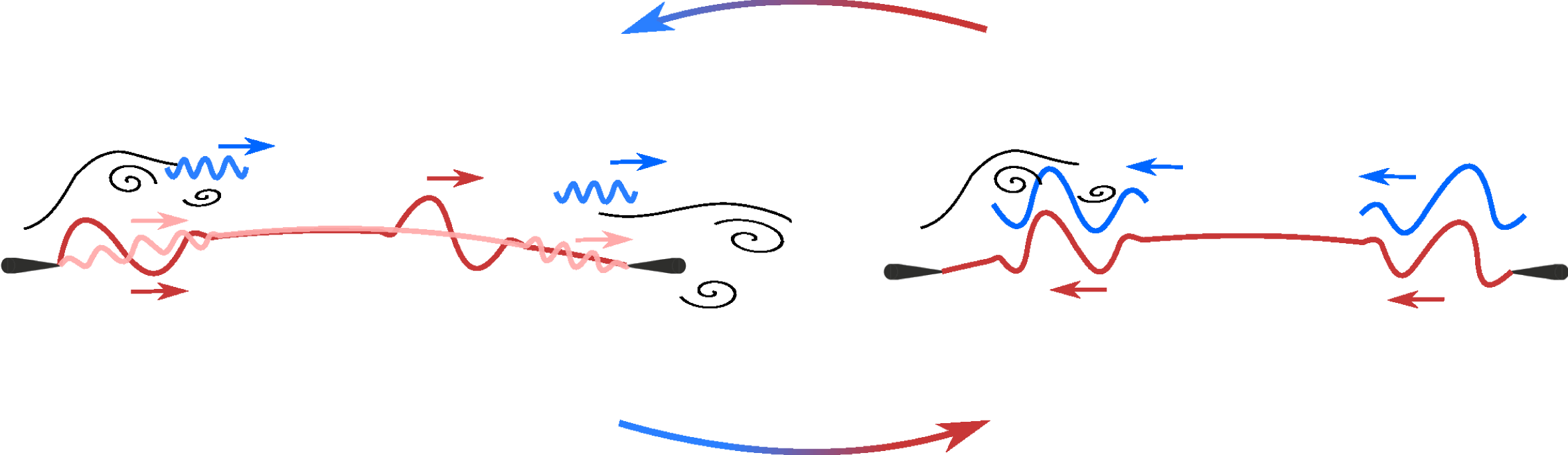
A schematic of the fluid–structure coupling mechanism at the dominant frequency
 $St\approx 0.9$
is presented in figure 11. The strong correlation between pressure and deflection indicates that the fluctuations of upstream-travelling pressure and membrane deflection occur on the same time scale, corresponding to the membrane second mode of oscillation. Travelling waves, with wavelength corresponding to the second structural mode, travel along the membrane from the LE to the TE (red waves in the sketch). When these waves are reflected from the TE support and travel upstream through the membrane, they seem to promote pressure fluctuations that also travel upstream with the same low phase velocity, far from the acoustic wave propagation speed (blue waves in the sketch). The same frequency was found to be associated with pressure fluctuations occurring not only on the aerofoil surface but also in the shear layer above the recirculation bubble and in the flow separation and vortex merging region around the TE. Therefore this type of wave, reflecting and propagating forwards and backwards on the membrane, seems to feed upstream-travelling pressure waves and vortex shedding that in return feed the membrane vibration, making this vibration frequency the most relevant in the fluid–structure interaction coupling. The same kind of phenomenon might occur with the vortex shedding and membrane vibration at
 $St=2.7$
, although this has not been clearly revealed by this investigation.
Finally, the cross-correlations between pressure and deflection at the location of maximum deflection r.m.s. for the full pressure and the downstream and upstream components in figures 7(b), 8(b), 10(b) show that pressure and deflection at the same location are instantaneously anti-correlated in all cases. This seems to agree with the findings of Bleischwitz et al. (Reference Bleischwitz, de Kat and Ganapathisubramani2016), where they found a positive correlation between deflection and lift coefficient, as an increase in lift would be expected to be related to a decrease in pressure on the aerofoil upper surface.
Conceptual sketch of the coupling mechanism. Red tones indicate deflection waves, blue tones indicate pressure waves.

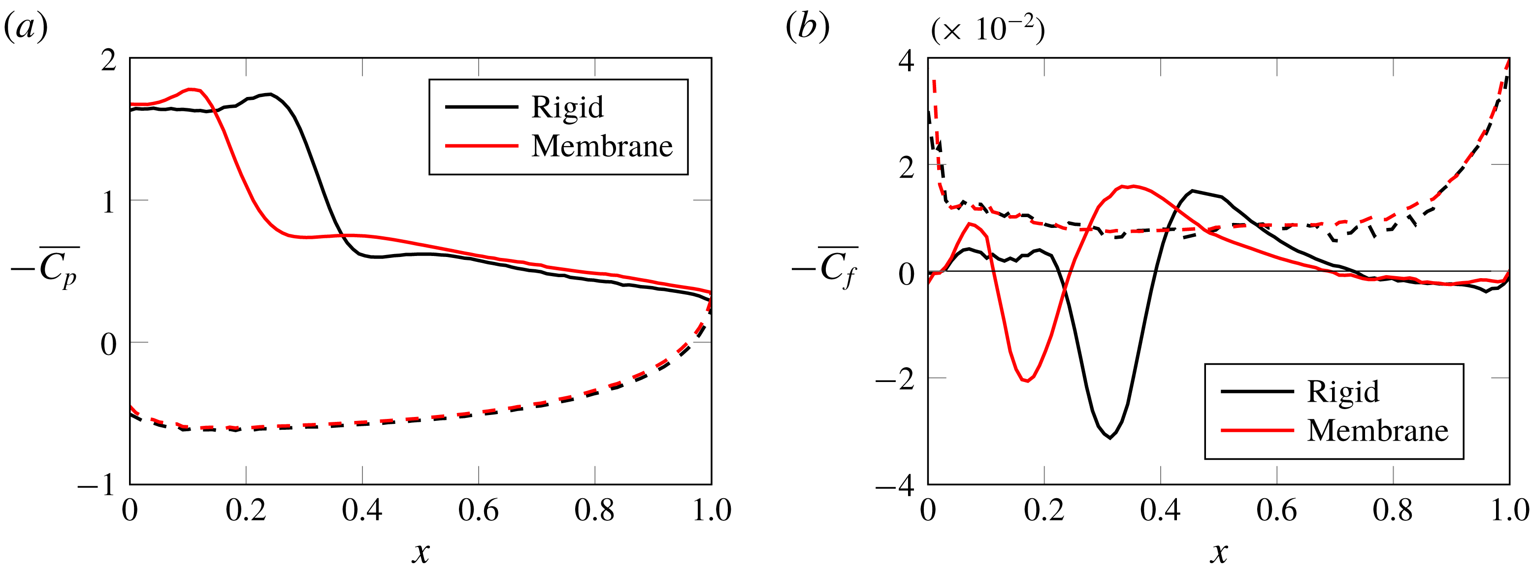
Comparison of (a) mean pressure coefficient (
 $\overline{C_{p}}$
) and (b) mean skin friction coefficient (
 $\overline{C_{f}}$
) for the rigid and membrane aerofoil. Dashed lines indicate the lower surface of the aerofoil.

Wavenumber–frequency spectrum of the pressure fluctuations on the upper surface of the rigid aerofoil along the streamwise location. Lines corresponding to free-stream propagation velocity (——),
 $50\,\%$
of the free-stream propagation velocity (
 $\cdots \cdots$
) and sound propagation velocity (- -) are included as reference.

5 Comparison with rigid aerofoil and causes of drag increase
An additional simulation for a rigid cambered aerofoil with the shape of the mean deflection of the flexible membrane was carried out to enable a direct evaluation of the effect of the membrane shape fluctuations. Before investigating the differences in the dynamics, the mean pressure distribution and mean skin friction along the aerofoil chord are shown in figure 12. The mean
 $C_{p}$
curves for the rigid case in figure 12(a) shows that the suction peak moves significantly downstream, although the maximum
 $-\overline{C_{p}}$
value and values downstream of the peak appear to be very similar to the flexible case. According to the zero crossing of the mean skin friction coefficient in figure 12(b), the recirculation bubble in the rigid case is slightly enlarged. The separation point is located at
 $x=0.22$
and the reattachment point at
 $x=0.4$
, which are both farther downstream compared to the flexible membrane. The separation location in the aft section of the aerofoil is similar in both cases, around
 $x=0.7$
. Similar effects were observed in the comparison between rigid cambered and flexible membrane aerofoils at higher angle of attack and lower Reynolds number by Gordnier (Reference Gordnier2009).
In the rigid case, it is observed that the vortex shedding starting in the recirculation area close to the LE becomes regular and periodic. The wavenumber–frequency spectrum of the upper surface pressure for the rigid case is depicted in figure 13. The branch of the spectrum corresponding to downstream-travelling waves is much cleaner and with smaller slope than in the flexible case. The dominant frequency
 $St\approx 1.2$
and its subharmonics are clearly distinguished. Comparing these results with those from the flexible wing, it is observed that the displacement of the membrane introduces a variety of additional frequencies into the flow. When there are no structural vibrations, the branch of the spectrum corresponding to upstream-travelling waves with phase velocity
 $C_{ph}\approx -1$
vanishes and the only indication of upstream-propagating pressure waves appears at the phase speed corresponding to acoustic waves. This supports the previous analysis about the fluid–structure coupling (§ 4.3).
Finally, aerodynamic coefficients are compared for the rigid and flexible aerofoils in table 1. Although the vibration of the membrane seems to improve slightly the averaged lift force, the dynamic effect is disadvantageous for the drag. The flexible aerofoil has a drag coefficient that is
 $27.4\,\%$
higher than the rigid one, making the membrane aerofoil significantly aerodynamically less efficient than the rigid one. According to the study of flow over a wall undergoing streamwise travelling wave motion by Shen et al. (Reference Shen, Zhang, Yue and Triantafyllou2003), positive wave propagation velocities smaller than or equal to the free-stream flow velocity tend to reduce separation and introduce changes in the mean pressure distribution that result in a reduction of drag. According to their study, the drag decreases monotonically as the phase velocity of the wave increases. The opposite is found for negative wave propagation velocity. Upstream wall movement induces more reverse flow and enhances separation, resulting in a greater drag force. Although the amplitude of the wavy wall that they considered is one order of magnitude larger than the amplitude of the membrane vibrations in the present study, similar behaviour might still apply. Therefore, although the downstream-travelling waves in the membrane could be beneficial regarding drag, at the low angle of attack considered for the aerofoil here, the upstream-propagating waves on the membrane and their induced flow pressure fluctuations seem to have a larger influence on the drag increase. In particular, at the specific time instances of the highest instantaneous drag, the travelling waves in the membrane reflected from the TE and travelling back upstream increase the curvature on the aft section of the aerofoil in a sort of inverted second mode deformation. This movement pushes the flow over the surface up and backwards, slowing it down and promoting vortex merging and mixing. Hence, the flow loses momentum and the pressure increases, which might be the cause of the instantaneous increase in drag. An animation of the vorticity field together with deflection, pressure and aerodynamic coefficients fluctuations illustrating the facts just described can be found at http://dx.doi.org/10.5258/SOTON/397076.
Aerodynamic characteristics of the rigid and flexible aerofoils, including the variation in percentage of lift (
 $C_{l}$
), drag (
 $C_{d}$
) and aerodynamic efficiency (
 $L/D$
) with respect to the rigid case. Subscripts
 $p$
and
 $\unicode[STIX]{x1D70F}_{w}$
indicate respectively the contribution from pressure and skin friction.

6 Fluid–structure coupling in membrane aerofoil under fully developed 3D flow
In this section the fully developed 3D flow at Reynolds number
 $Re=10\,000$
and its effect on the fluid–structure coupling are investigated. An infinite-span membrane wing that is elastic in the streamwise direction but non-deformable in the spanwise direction is simulated. This is a direct extension of the 2D membrane aerofoil problem studied in the previous section to a 3D case, where the flow develops 3D characteristics and the wing structure is representative of materials with non-homogeneous structural stiffness in the
 $z$
-direction, as could be the case of material mimicking wing muscles, or membrane wings with supporting ribs preventing spanwise deformation.
Previous computational studies of membrane aerofoils at Reynolds numbers up to
 $Re=10\,000$
suggested that this Reynolds number might be the upper limit of the 2D laminar flow regime (Gordnier Reference Gordnier2009; Jaworski & Gordnier Reference Jaworski and Gordnier2012). Experimental work on membrane aerofoils (Hu, Tamai & Murphy Reference Hu, Tamai and Murphy2008; Rojratsirikul et al.
Reference Rojratsirikul, Wang and Gursul2009, Reference Rojratsirikul, Wang and Gursul2010; Arbós-Torrent et al.
Reference Arbós-Torrent, Ganapathisubramani and Palacios2013) and also the simulations from Gordnier & Attar (Reference Gordnier and Attar2009) have focused on higher Reynolds numbers. However, to the best knowledge of the authors, no direct comparison has been made so far on the differences or similarities between the flow–structural coupling with and without the restriction to 2D flow. In the following, characteristics of the 3D fluid/2D structural model problem are analysed using the techniques presented in the previous sections, focusing on the mean and unsteady behaviour, including characteristics in the frequency and wavenumber–frequency domains. These results are compared to the results from the 2D simulations in order to understand if the same coupling mechanisms are still present when local 3D flow effects are incorporated into the aerofoil fluid–structure interaction problem.
6.1 Fully developed 3D flow
Autocorrelation functions for the three momentum components
 $\unicode[STIX]{x1D70C}u_{1}$
,
 $\unicode[STIX]{x1D70C}u_{2}$
,
 $\unicode[STIX]{x1D70C}u_{3}$
, in the wake,
 $x=1.5$
.

Side and top view of the instantaneous isosurfaces of
 $Q=250$
coloured with the velocity magnitude at the simulation non-dimensional time
 $t=66.25$
.

The 3D simulation was initialised with the solution from the 2D case, upon which initial spanwise velocity perturbations were superimposed in the full fluid domain in the form of white noise with a maximum amplitude of order
 $10^{-8}$
. The linear stages of the 3D disturbances growth were reported in Serrano-Galiano & Sandberg (Reference Serrano-Galiano and Sandberg2015). After initialisation, the simulation was run for a time long enough to allow the full 3D flow evolution and the collection of converged statistical data. The simulation was carried out using 32 Fourier modes (equivalent to
 $N_{Z}=2\times \text{number of modes}+2=66$
), comparable to the resolution of previous DNS of aerofoils (Jones et al.
Reference Jones, Sandberg and Sandham2008), a domain width of
 $L_{Z}=0.5$
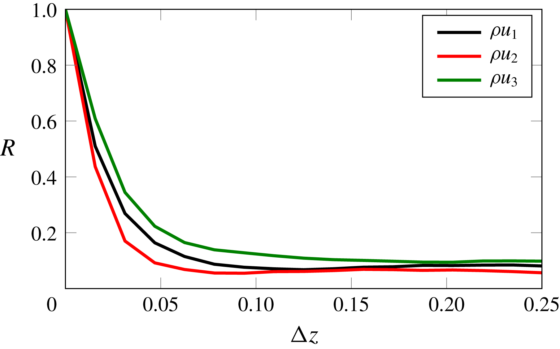
and the same in-plane grid as for the 2D case. The autocorrelation of the three velocity components is shown in figure 14 to assess the suitability of the domain size in the spanwise direction. The plot depicts the autocorrelation function as a function of spanwise distance over half of
 $L_{Z}$
(as the computational domain has symmetric boundary conditions in the spanwise direction). The correlation values quickly decay with
 $\unicode[STIX]{x1D6E5}_{z}$
, indicating that a spanwise width of
 $L_{Z}=0.5$
is sufficient. On the structural side, the forcing term
 $\unicode[STIX]{x0394}p$
at each time step corresponds to the spanwise spatial average of the pressure difference between the upper and lower surfaces of the membrane. The 2D geometry of the deflected membrane, calculated using
 $\unicode[STIX]{x0394}p$
, is updated at the end of each time step and extruded in the spanwise direction so that only the flow is allowed to develop in three dimensions.
Isosurfaces of
 $Q=250$
in black with isosurfaces of pressure varying from
 $p=16.8$
to
 $p=17.8$
as shown in the colour bar, at the simulation non-dimensional time
 $t=66.25$
.

In order to investigate the flow development, isosurfaces of the second invariant of the velocity gradient tensor,
 $Q$
, are visualised in figure 15. The instantaneous
 $Q$
-isosurfaces are for a constant value
 $Q=250$
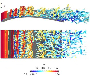
and coloured with the velocity magnitude. These isosurfaces show that large 2D rollers are still clearly visible near the LE, despite the 3D perturbations. At approximately
 $30\,\%$
of the chord, these large flow structures develop spanwise fluctuations with a wavelength
 $\unicode[STIX]{x1D706}\approx L_{Z}/8=0.0625$
, coinciding with the first harmonic of the most amplified mode observed in Serrano-Galiano & Sandberg (Reference Serrano-Galiano and Sandberg2015). As they are convected downstream over the wing surface they break down and the outer shear layer of the recirculation bubble rolls up into smaller structures. In the aft section of the aerofoil the topology of the flow has significantly changed from large spanwise-oriented vortices to small longitudinal vortices, resembling in some areas the hairpin-like and arch-like structures found in turbulent flows by Dubief & Delcayre (Reference Dubief and Delcayre2000). It is also noticed that, differently to the 2D case, there are no vortices rolling up from the lower surface to merge with the upper vortices in the wake. This might be due to an average increase in pressure over the TE compared to the 2D case, as will be seen later in the averaged pressure distribution (§ 6.2.1).
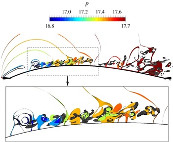
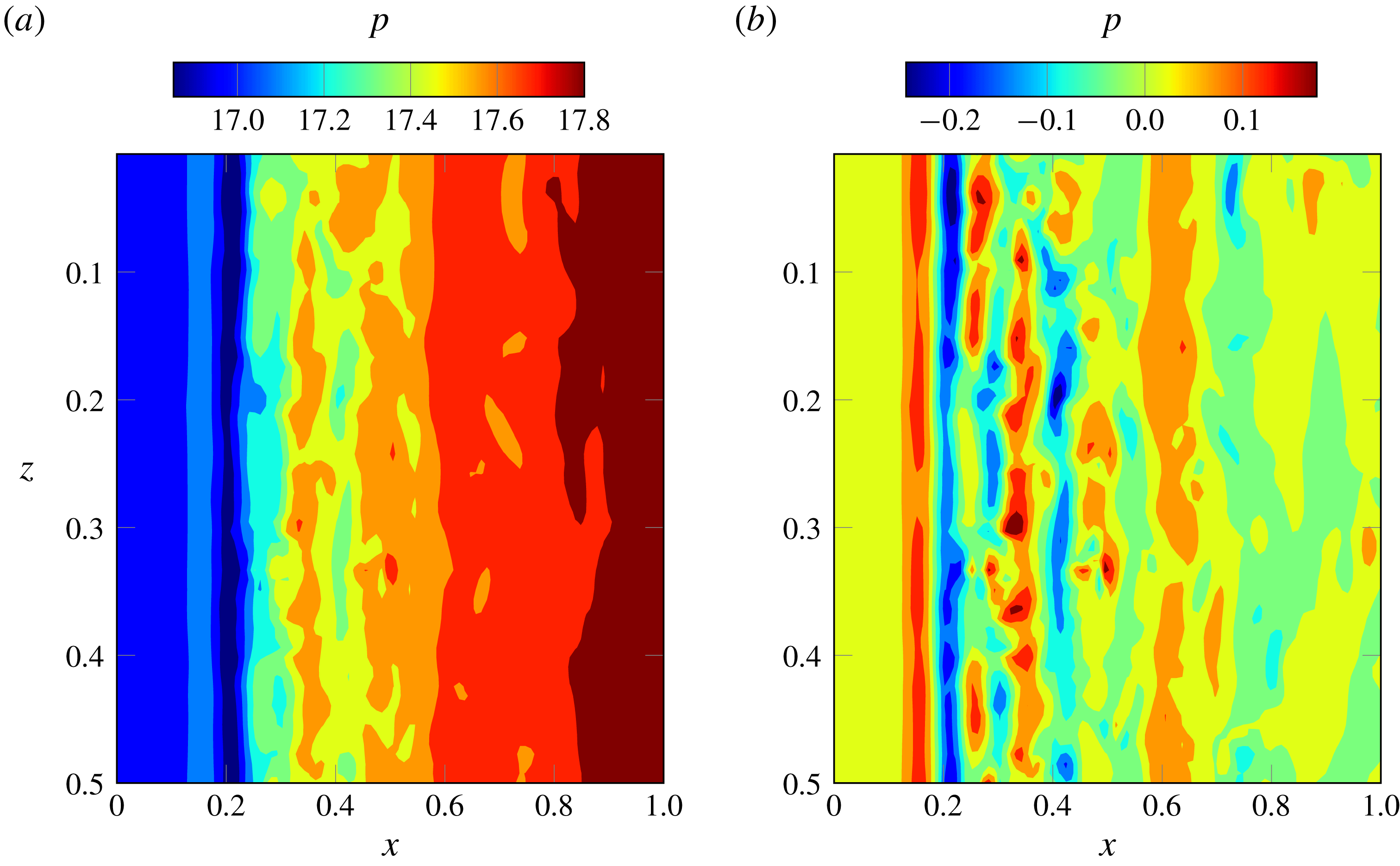
Besides the clear development of three-dimensionality and small-scale flow structures, in the side view in figure 15 it is observed that these small structures move downstream clustered in discrete regions along the chord in a similar fashion to the vortices observed in the 2D case (figure 3), maintaining a certain spanwise coherence. This is reflected in the pressure variation on the upper surface of the membrane. Figure 16 shows the alignment of the
 $Q$
-isosurfaces with isosurfaces of pressure in a thin portion of the flow domain over the membrane surface between
 $z=0$
and
 $z=0.01$
. Figure 17(a) shows instantaneous pressure contours on the wing upper surface, corresponding to the same time instant of the
 $Q$
-isosurfaces in figure 15, while figure 17(b) depicts instantaneous pressure fluctuations relative to the time-averaged pressure at each
 $x$
-,
 $z$
-location. The pressure on the membrane surface appears to be characterised mainly by variations along the streamwise direction, without strong variations in the spanwise direction. Low values of the pressure fluctuations appear in spanwise stripes aligned with the region of clustered vortical structures.
(a) Instantaneous pressure and (b) pressure fluctuations, both on the upper surface of the membrane at the simulation non-dimensional time
 $t=66.25$
.

As mentioned before, the coupling between the flow and the structural solver is achieved via the instantaneous spanwise-averaged pressure difference. The adequacy of this assumption is confirmed by the lack of three-dimensionality in the instantaneous surface pressure distribution shown in figures 17(a) and 17(b). This might also suggest that, in the case of a wing with flexibility also in the spanwise direction, the pressure fluctuations in the streamwise direction would prevail over the spanwise fluctuation, causing a membrane forcing with variations predominantly in the chordwise direction. This would be expected to cause essentially streamwise membrane fluctuations too. In such a case the fluid–structure coupling results would be expected to be similar to the results from the present section. Nevertheless, it would be interesting in the future to compare the present results with a case with fully 3D membrane motion.
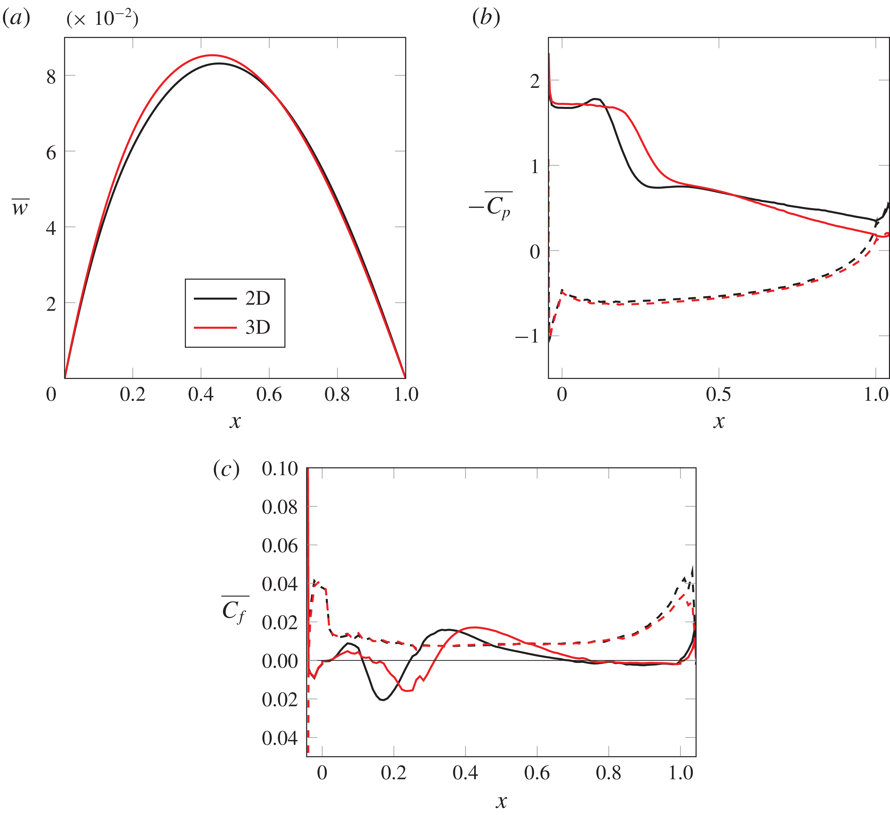
Comparisons of mean deflection (
 $\overline{w}$
), surface pressure coefficient (
 $\overline{C_{p}}$
) and skin friction coefficient (
 $\overline{C_{f}}$
) for the 2D and 3D simulations. The dashed line indicates the lower surface of the aerofoil.

6.2 Comparison of 2D–3D fluid–structure interaction
6.2.1 Mean behaviour
The mean quantities presented in this section are computed by averaging in time over 21 non-dimensional time units (4000 equispaced data samples) and additionally averaging the flow field data in the spanwise direction. Figure 18(a) shows the mean membrane deflection along the chord
 $(\overline{w})$
. The maximum mean deflection is found to be
 $2.4\,\%$
higher in the 3D case compared to the 2D case, and the point of maximum deflection moves slightly upstream, from
 $x=0.45$
in 2D to
 $x=0.43$
in 3D. This is consistent with the differences in mean pressure distribution observed in figure 18(b). The mean pressure coefficient
 $(-\overline{C_{p}})$
curve on the upper surface of the 3D case shows a pressure plateau that is characteristic of a laminar separation bubble, as described in Horton (Reference Horton1968), which is longer than in the corresponding 2D case. At the same time, higher pressure values in the last
 $30\,\%$
of the chord are observed for the 3D case compared to the 2D aerofoil. Both of these phenomena cause the membrane to be ‘pulled’ slightly further forward by the flow in the 3D case.
The mean skin friction coefficient
 $(\overline{C_{f}})$
is depicted in figure 18(c). The zero crossing of the
 $\overline{C_{f}}$
curve on the upper surface of the 3D case indicates a recirculation bubble that extends from
 $x=-0.037$
to
 $x=0.30$
, which is larger than the 2D separation bubble. According to this curve, inside the recirculation bubble there is a region of counter-rotating flow indicated by the positive values of
 $\overline{C_{f}}$
between
 $x=-0.02$
to
 $x=0.14$
. However, in the
 $(-\overline{C_{p}})$
curve of the 3D case no localised decrease in pressure is found before the steep pressure increase near the reattachment point. After the separation bubble, reattachment takes place. However, the peak skin friction levels are very similar in the 2D and 3D cases. Despite the transition to turbulent flow away from the surface, it appears that a near-wall turbulence regeneration cycle (Jiménez & Pinelli Reference Jiménez and Pinelli1999) does not form and the flow subsequently separates close to the TE, at
 $x=0.74$
, in essentially a laminar fashion. The present results are unusual, as the separation bubble in a 3D case would be expected to shorten due to the breakdown of the flow into smaller vortices. The reason for a longer 3D bubble seems to be in the interaction between the flow and the membrane. It was found in the 2D comparison in § 5 that the vibration of the flexible membrane reduced the length of the averaged bubble compared to the bubble in the rigid case. Since in the 2D case the amplitude of the fluctuations of the membrane is higher than in the 3D case (see § 6.2.2), an effect similar to the rigidity of the membrane seems to be responsible for the longer bubble in the 3D case.
 $x$
-
 $t$
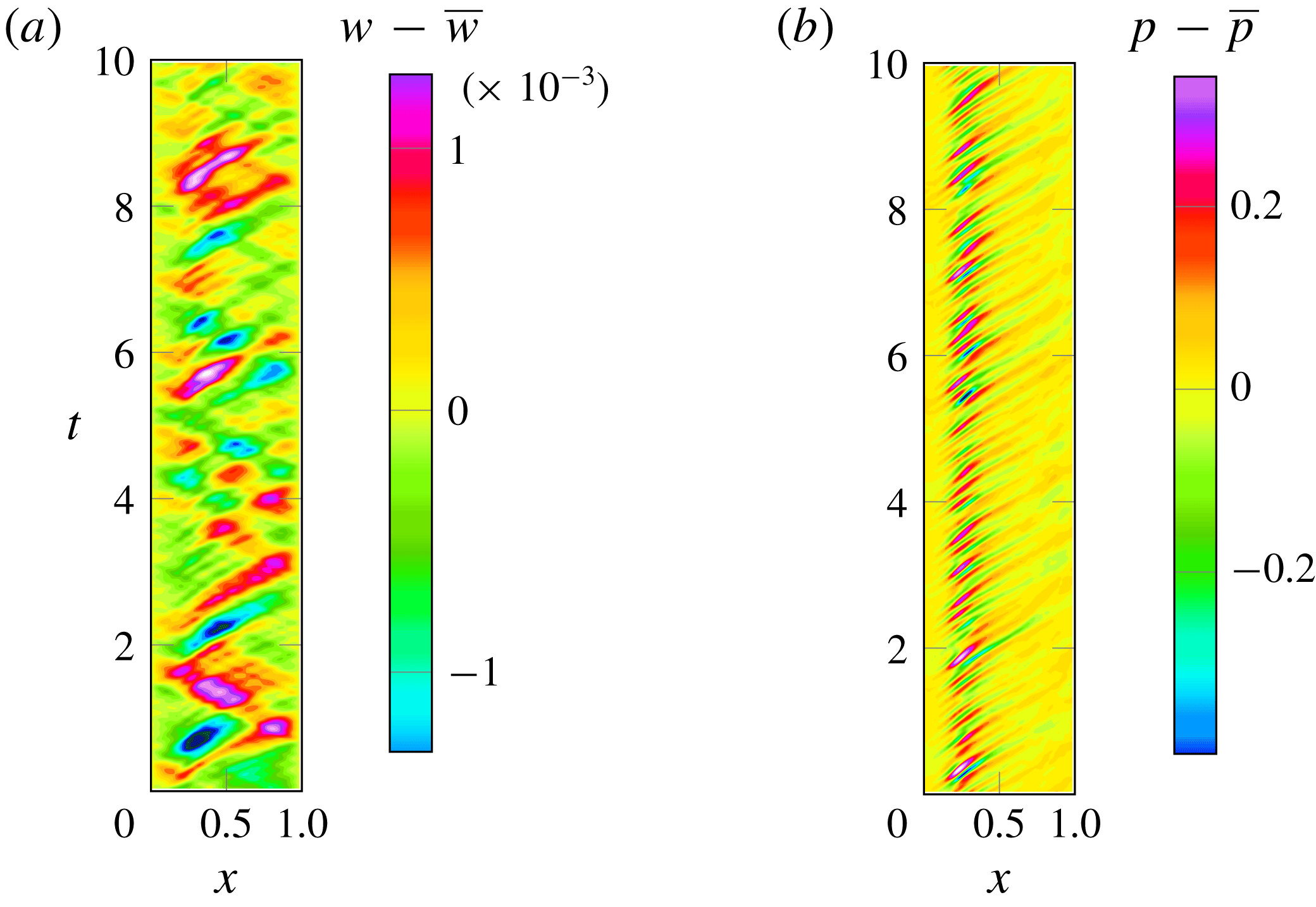
-diagrams of (a) fluctuations of the membrane deflection (
 $w-\overline{w}$
) and (b) the span-averaged pressure on the upper surface (
 $p-\overline{p}$
) for the 3D simulation.

6.2.2 Time-dependent behaviour
Additionally to the mean features of flow and structure, the effect of the 3D flow development on the dynamic behaviour is also considered. Recall that the membrane simulated here has the same shape and time-dependent behaviour at all
 $z$
-locations, since the membrane equation is a one-dimensional model and the solution is extruded in the spanwise direction. However, the flow field is the solution of a fully 3D problem and therefore variations occur across the span. Since the coupling between the flow and the membrane occurs through the pressure difference between the upper and lower surface, averaged in the spanwise direction, the time-dependent behaviour of pressure is investigated in the same sense, i.e. all the dynamic analysis in the pressure signal in this section is carried out for the pressure time signal at each
 $x$
-location with averaging across the span.
The pressure footprint of the span-averaged vortices on the membrane upper surface can be observed in the pressure
 $x$
-
 $t$
-diagrams in figure 19. The contours show the span-averaged membrane deflection and upper surface pressure fluctuations at 100 locations along the chord. The pressure fluctuations are dominated by downstream-propagating waves with half the amplitude of the fluctuations observed in the 2D case (notice the different scale in the colour bar with respect to the 2D cases plotted in figure 3). The highest amplitudes are observed in the first half of the chord, caused by the large coherent vortical structures detaching from the recirculation bubble. As these structures are convected downstream they break into smaller structures that have a smoother footprint on the membrane surface pressure. The short distance in time between the low-pressure fringes in this plot approximately coincides with the time period of the dominant frequency found in the pressure spectrum,
 $St=4.6$
. This confirms the higher frequency of the LE vortex shedding in the 3D flow compared to the 2D case. The lower amplitude of pressure fluctuations induces lower-amplitude membrane fluctuations shown in the
 $x$
-
 $t$
-diagram of the deflection fluctuation time signal (figure 19
a). The contours of deflection fluctuations reveal downstream and upstream propagating waves patterns very similar to the behaviour found in the 2D simulation, but with amplitudes that are eight times lower.
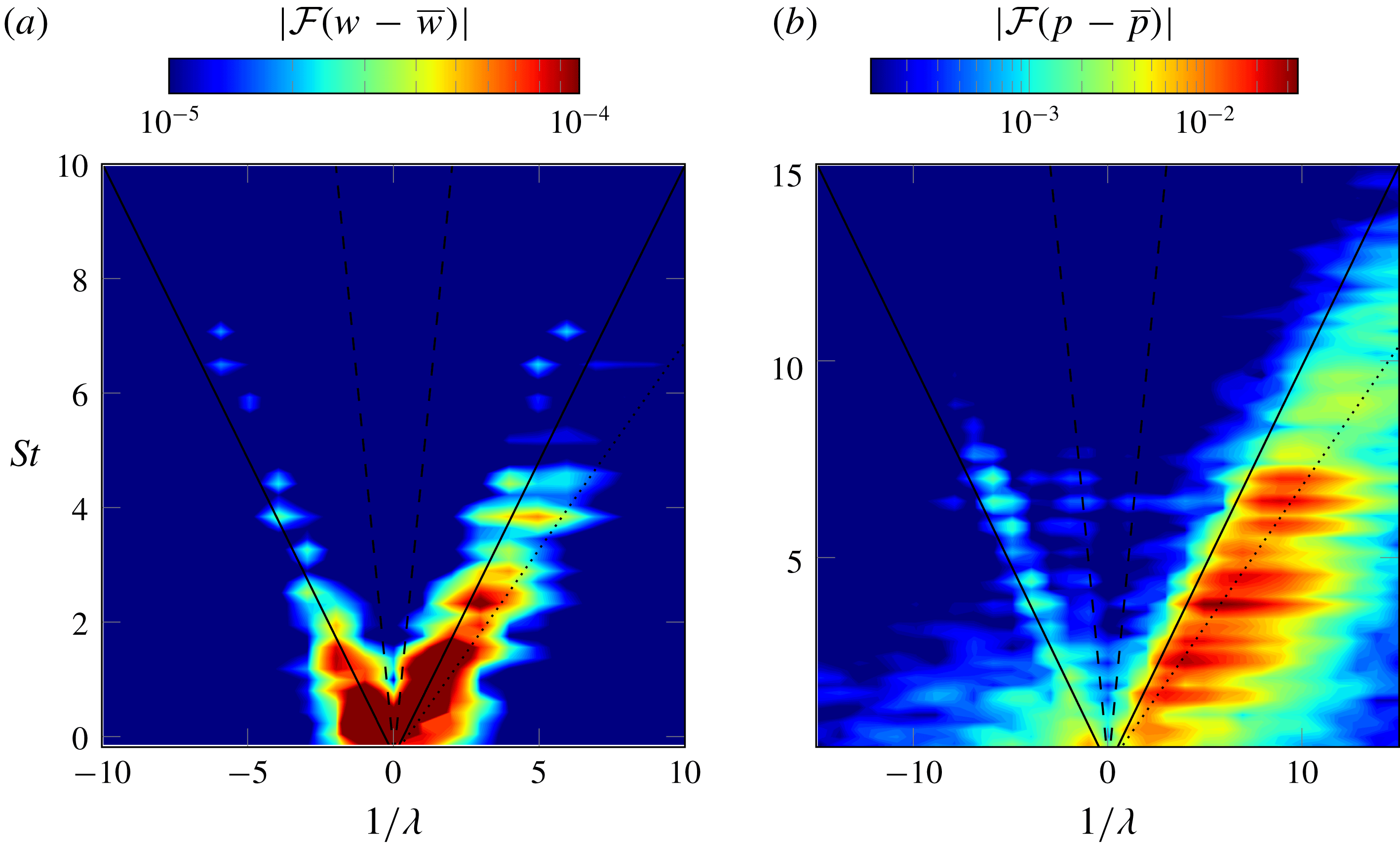
Wavenumber–frequency spectra of (a) membrane fluctuations (
 $w$
) and (b) pressure (
 $p$
) fluctuations along the upper surface of the membrane for the 3D simulation. Lines corresponding to free-stream propagation velocity (——),
 $70\,\%$
of the free-stream propagation velocity (
 $\cdots \cdots$
) and sound propagating velocity (- -) are included as reference.

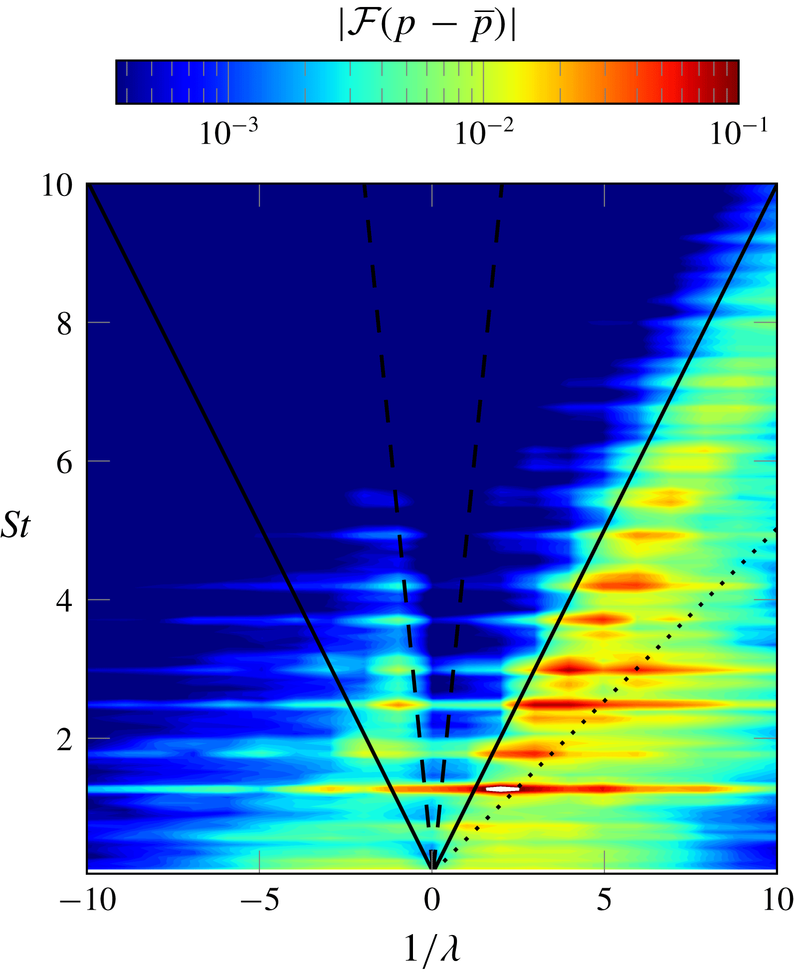
The time- and space-dependent data of deflection and upper surface pressure (averaged in span) were double-Fourier-transformed to obtain the wavenumber–frequency spectra for the 3D case. Figure 20 was produced following the same procedure as in the 2D case described in § 3.1 and shows the Fourier coefficients amplitudes as a function of the Strouhal number,
 $St$
, and the inverse of the non-dimensional wavelength
 $1/\unicode[STIX]{x1D706}$
. In the deflection spectrum (figure 20
a) two almost symmetric branches are again found for the 3D case, corresponding to the upstream- and downstream-propagating waves. Both branches show lower amplitude than in the 2D case and the energy is concentrated in low frequencies and low wavenumbers related through the phase velocity
 $c_{ph}=\sqrt{T_{s}/(\unicode[STIX]{x1D70C}_{s}h)}\approx 1.3$
. The phase velocity computed in the 3D case is higher than that calculated in the 2D case due to the slightly higher 3D mean deflection, which induces higher tension in the membrane. The highest peaks in the spectra of the membrane fluctuations are found at
 $St=0.37,0.83,1.38,1.75$
, which seem to correspond to a first, second, third and fourth mode of the membrane, respectively. Some indication of significant energy content is also found at frequencies
 $St=2.5,3.5,4.0$
and
 $4.6$
, coinciding with the dominant frequencies found in the pressure spectra.
The wavenumber–frequency spectrum for the pressure (figure 20
b) shows a dominant downstream branch with a lower slope, of approximately 0.6, compared to the 2D case downstream branch in § 3.1. This appears to be an indication of slower convection of the dominant structures over the membrane for the 3D case. The dominant frequencies in the pressure spectra are found at approximately
 $St=0.83,1.84,2.58,3.5,4.04,4.6$
, with the highest energy contained in the higher frequencies. The membrane oscillations are found to be dominated by approximately the same frequencies as in the 2D case and influence the pressure fluctuations. However, the vortex shedding frequency in the 3D flow is almost double that of the 2D case. A weaker upstream branch is also observed with a slope of approximately
 $-1$
that represents upstream-travelling pressure waves similar to the spectrum found in the 2D case. This branch coincides with the combination of frequencies and wavenumbers found in the upstream branch of the deflection spectrum and, from the analysis carried out in § 4, it can be argued to be caused by the coupling between the membrane and the flow. Therefore, it can be concluded that the main effect of the flow three-dimensionality is a decrease in the surface pressure fluctuations intensity, and consequently a decrease in deflection fluctuation amplitudes. However, the coupling mechanism found in the 2D results is still applicable for the 3D flow, with the structural parameters simulated here.
7 Conclusions
Direct numerical simulations of a membrane aerofoil with an angle of attack of 8 degrees and
 $Re=10\,000$
have been carried out starting with 2D cases. The results suggest that the fluid–structure coupling introduces upstream-propagating pressure waves travelling from the TE to the LE of the aerofoil different from the acoustic wave propagation speed. The analysis of space- and time-dependent data of pressure and deflection in the wavenumber–frequency domain has shown that pressure fluctuations over a wide range of frequencies are redistributed into a few discrete low frequencies of the membrane response. The vibration of the membrane under the flow forcing has the form of travelling waves in the positive and negative
 $x$
-direction. The pressure fluctuations in the surface are dominated by pressure waves travelling downstream. However, a branch of high energy content was found in the wavenumber–frequency spectrum, corresponding to upstream-propagating pressure waves with a phase speed very similar to the phase speed of the structural waves propagating upstream on the membrane, after reflecting on the TE support. The high correlation between upstream-propagating pressure and deflection confirms the origin of the upstream-travelling pressure waves to be in the fluid–structure interaction, for which a mechanism has been proposed.
The upstream-propagating waves are suggested to be the cause of the loss in aerodynamic efficiency on a membrane aerofoil compared with a rigid cambered aerofoil. When the dynamic behaviour is suppressed and the aerofoil is rigid with the same shape as the flexible aerofoil mean deflection the only upstream-propagating pressure waves remaining are waves with a phase speed in the acoustic range. The suppression of upstream-propagating waves in the membrane, and consequently in the pressure field, is suggested as a possible measure to alleviate the loss of aerodynamic efficiency in membrane aerofoils at low angle of attack.
When the simulation was extended to three dimensions, whilst retaining the 2D structural model, the fully developed flow at
 $Re=10\,000$
showed a breakdown of the large quasi-2D rollers generated at the LE into smaller 3D vortices as the flow moves downstream over the membrane. The smaller vortices move in the streamwise direction clustered into coherent spanwise structures, which causes the pressure on the membrane surface to change mainly in the streamwise direction. Thus the fluid–structure coupling in the 2D and 3D cases simulated was found to have similar characteristics.
Acknowledgements
The authors are grateful for the funding provided by EPSRC under grant no. EP/J001465/1. Acknowledgement is given to the UK Turbulence Consortium for the provision of computational time on the UK national computer ARCHER under grant no. EP/L000261/1. Data statement: supporting data in the form of dimensionless deflection, pressure and skin friction coefficients are available from the University of Southampton repository at http://dx.doi.org/10.5258/SOTON/397076.