1. Introduction
The study of turbulent boundary layers has historically been a focal point in the realm of wall-bounded turbulent flows, in both past and contemporary researches. However, a predominant majority of these studies have centred around the flat plate configuration or planar turbulent boundary layer. Nonetheless, there exists a multitude of engineering challenges and practical applications that involve the cylindrical turbulent boundary layer. These applications span a wide range, from the vibration of towed submerged cables to the manufacturing of polymer fibres, and even extend to the aerodynamics of flying missiles. It is worth noting that in many real-world applications, the radius of the cylindrical object is considerably smaller than the thickness of its turbulent boundary layer. This poses significant curvature effects on both turbulence statistics and coherent structures. In the following, we will use the abbreviation TBL to denote the planar turbulent boundary layer over a flat plate, and ATBL to denote the axisymmetric turbulent boundary layer along a cylinder, to be consistent with the notations in the literature.
In the ATBL, there is one more length scale besides the boundary layer thickness (
 $\delta$
), namely the cylinder radius (
 $a$
). Therefore, different from the TBL, there are two key dimensionless parameters often used in studies of the ATBL (Neves, Parviz & Moser Reference Neves, Moin and Moser1994): the curvature parameter
 $\delta /a$
, and the radius in wall units
 $a^+=au_\tau /\nu$
, where
 $u_\tau$
is the friction velocity, and
 $\nu$
is the kinematic viscosity. According to the values of
 $\delta /a$
and
 $a^+$
, the flow could be divided into three regimes (Piquet & Patel Reference Piquet and Patel1999): (i) the regime with large
 $\delta /a$
and large
 $a^+$
, where the boundary layer along a long slender cylinder is almost all a wake-like flow; (ii) the regime with small
 $\delta /a$
and large
 $a^+$
, where the boundary layer develops along a thick cylinder and experiences little curvature effect, behaving like a flat plate boundary layer; (iii) the regime with large
 $\delta /a$
and small
 $a^+$
, where the flow is similar to that of an axisymmetric wake with an inner boundary layer – in this case, the TBL has large thickness, and the inside turbulent activities are under the significant influence of the transverse curvature. The presently studied flow falls into the third regime.
Extensive research has been conducted on the distribution of skin friction coefficients along slender cylinders in the ATBL due to its engineering significance. Glauert & Lighthill (Reference Glauert and Lighthill1955) used the Pohlhausen method and asymptotic series solution, and gave the distributions of the skin friction along the cylinder within
 $0.04\lt \nu x/Ua^2\lt 100$
, where
 $x$
is the distance from the front edge, and
 $U$
is the free-stream velocity. Monte et al. (Reference Monte, Sagaut and Gomez2011) extended the FIK identity (Fukagata, Iwamoto & Kasagi Reference Fukagata, Iwamoto and Kasagi2002) to the ATBL to discern the contributions of viscous and turbulent components to the skin friction, giving
 $C_f=2/(2.56\ln[Re_a\ln(1+\delta /a)]-2.53)^2$
within
 $311\lt Re_a\lt 10\,000$
and
 $1\lt \delta /a\lt 300$
. Jordan (Reference Jordan2013) also conducted a triple integration of the governing equations for the ATBL, and proposed a skin friction coefficient model covering
 $482\lt Re_a\lt 92\,310$
and
 $1.88\lt \delta /a\lt 42.5$
. Kumar & Mahesh (Reference Kumar and Mahesh2018) derived the momentum integral equation for the zero-pressure-gradient ATBL, and gave
 $C_f=2(\theta /\delta )(1+\theta /a)({\rm d}\delta /{\rm d}x)$
. Very recently, Ali & Dey (Reference Ali and Dey2023) applied the boundary layer approximation and found that the eddy turnover velocity is linked to the second-order structure function. They finally obtained a scaling law of the Reynolds shear stress and scaled the skin friction coefficients as
 $C_f\sim [Re_a\ln (1 + \delta /a)]^{-1/4-3\alpha _0/8}$
, where
 $\alpha _0$
represents a certain expansion exponent. This scaling agrees well with various experimental and numerical data under different flow parameters within
 $140\lt Re_a\lt 92\,310$
and
 $0.16\lt \delta /a\lt 300$
.
The influences of
 $a^+$
and
 $\delta /a$
were taken into account when determining the the mean velocity profile. Richmond (Reference Richmond1957) carried out a series of experiments with
 $\delta /a=2$
and
 $a^+=10{-} 76$
, and introduced a scaling approach for the mean velocity profile by replacing the wall-normal coordinate
 $y^+$
in the expression for the TBL with
 $y^+ (1+y^+/2a^+)$
for the ATBL. On the other hand, Rao (Reference Rao1967) proposed a form of double-logarithmic distribution for the mean velocity profile,
 $U^+ = A\ln[y^+\ln(r/a)]+B$
, for the ATBL with
 $\delta /a\approx 4$
and
 $a^+\approx 1600$
, where
 $A$
and
 $B$
are constants depending on the streamwise position and cylinder radius. Willmarth & Yang (Reference Willmarth and Yang1970) proposed distributions for mean velocity similar to those of Richmond (Reference Richmond1957) in the ATBL, with
 $\delta /a=1.38{-} 2.21$
,
 $a^+\approx 1517{-} 1601$
and
 $\delta /a=38.5{-} 77$
,
 $a^+\approx 5.3{-} 12.8$
. At higher Reynolds numbers, the slope and intercept of the logarithmic law of the mean velocity profile gradually approach fixed values (Afzal & Singh Reference Afzal and Singh1976), but a wake region persists. Afzal & Singh (Reference Afzal and Singh1976) provided asymptotic solutions for the ATBL at
 $a^+\approx 631 {-} 692$
and
 $\delta /a=0.6{-} 2.6$
. Lueptow et al. (Reference Lueptow, Leehey and Stellinger1985) used experimental data with
 $\delta /a=2{-} 50$
and
 $a^+=10{-} 134$
, and determined the values of the slope (
 $1/m$
) and the intercept (
 $n$
) for the log law
 $U^+=(1/m)\ln y^+ +n$
. For the mean velocity distribution of the ATBL, while the curvature effect has been taken into account by incorporating
 $1/a$
into the expressions, their universality is far from satisfactory because the coefficients still strongly depend on cylinder radius and flow Reynolds number.
Concerning the curvature effects on turbulence intensities, experimental research showed that they were profound in the outer region of the TBL, while numerical works disclosed that they were also significant in the near-wall region. Afzal & Singh (Reference Afzal and Singh1976) measured the axial velocity fluctuations and found that compared with the TBL, the axial turbulence intensity in the ATBL was weakened in the outer layer but kept the similar amplitude in the near-wall region. The same phenomenon was also reported by Luxton, Bull & Rajagopalan (Reference Luxton, Bull and Rajagopalan1984). Lueptow et al. (Reference Lueptow, Leehey and Stellinger1985) pointed out that when moving away from the wall, the Reynolds shear stress dropped more quickly in the ATBL than in the TBL. They also proposed a scaling
 $a/r$
to collapse the Reynolds shear stress at different
 $\delta /a$
ranging from 4.59 to 8.53. Lueptow (Reference Lueptow1990) attributed the large decrease of turbulence intensity in the outer region to the increased spreading of the flow field to larger circumferential length as moving further away from the cylinder wall. Neves et al. (Reference Neves, Moin and Moser1994) performed direct numerical simulations (DNS) of the turbulent flows between two concentric cylinders driven by the axial pressure gradient. They found that the three components of turbulence intensities scaled by
 $u_\tau$
decreased as the curvature parameter
 $\delta /a$
increased in the whole radial range, not only in the outer region as the former experimental research noted. A velocity scale was proposed based on the momentum equation to collapse the turbulence intensities in the near-wall region. Jordan (Reference Jordan2012) performed large-eddy simulations of ATBLs with
 $\delta /a=11{-} 73$
and
 $a^+=37{-} 62$
, and found that as the curvature parameter
 $\delta /a$
increases, the turbulence intensities normalised by the inner–outer mixed scale of
 $u_\tau U_\infty$
increase in both the near-wall and outer regions.
The transport of turbulent kinetic energy in the ATBL is also under the influence of the transverse curvature. Neves et al. (Reference Neves, Moin and Moser1994) analysed the proportions of different velocity components in turbulent kinetic energy of turbulent flows between two concentric cylinders, and attributed the increased fraction of axial component to the weakened inter-component energy transfer by the pressure–strain rate correlations in comparison with the TBL. Piquet & Patel (Reference Piquet and Patel1999) studied the Reynolds stress transport equations in the ATBL, and proposed that the production mechanism should be similar to that in the TBL, and the transverse curvature inhibits the energy transfer from the axial component to radial and circumferential components.
Experimental and numerical research have revealed that cylinders with small radii can support thick boundary layers, harbouring a multitude of active turbulent structures across the whole radial regions. Willmarth & Yang (Reference Willmarth and Yang1970) noted that the mean velocity profile appears much ‘fuller’ under the influence of cylinder curvature, suggesting that large-scale vortices may form in the outer region of the boundary layer, largely unaffected by the cylinder wall. Lueptow (Reference Lueptow1990) identified a burst cycle similar to other wall-bounded cases in the near-wall region that was responsible for turbulence generation. He highlighted the existence of structures moving from one side of the cylinder to the opposite side in the outer region, which may intensify the interaction between the outer flow and near-wall burst events. Additionally, he found that large-scale structures were observed in the outer region of the ATBL, suggesting that the wall may not play as significant a role in controlling coherent structures as it does in planar boundary layers. The high-speed velocity streaks similar to these low-speed ones of the planar case were observed in the ATBL with
 $a^+=42$
and
 $Re_a=879$
(Lueptow & Jackson Reference Lueptow and Jackson1991), which is evidence of the same important role of the burst cycle under the curvature effect. Neves et al. (Reference Neves, Moin and Moser1994) gave the instantaneous distribution of vorticity fluctuations, revealing the presence of different scales of vortical structures. They pointed out that the shear layer has almost the same length scale compared to the cylinder radius, and the scales of vortical structures are getting smaller with the increasing curvature. The near-wall coherent structures such as the low-speed streaks and vortical structures tended to be elongated in streamwise direction compared with lower transverse curvature and flat plate cases (Robinson Reference Robinson1991). Snarski & Lueptow (Reference Snarski and Lueptow1995) found that there were two main kinds of structures contributing to the wall pressure fluctuations in the ATBL. They gave a conceptual model describing the outline and frame of wall pressure and velocity using the space–time cross-correlation analysis. Piquet & Patel (Reference Piquet and Patel1999) emphasised the existence of large-scale structures that are larger than the scale of the cylinder radius distributed across the cylinder, and he thought this was due to less constraint by the curved wall than the planar wall. A larger curvature parameter
 $\delta /a$
leads to more active migration of the large-scale structures from one side of the cylinder to the other. Ohta (Reference Ohta2017) performed DNS for flow along the cylinder and investigated the geometry of the near-wall high- and low-speed velocity streaks. They found that the streaks exhibited similarities to those observed in flat plate cases, albeit with limited circumferential spacing and large curvature parameter, indicating that there existed certain universality in the characteristics of coherent structures along a cylinder.
As for the numerical simulation, there exist a certain number of studies related to ATBL. Neves et al. (Reference Neves, Moin and Moser1994) and Ohta (Reference Ohta2017) carried out DNS for turbulent flows between two concentric cylinders driven by streamwise pressure gradient. As a surrogate of the ATBL, this model provided an accurate approximation to the ATBL in the near-wall region. But it is statistically uniform in both streamwise and circumferential directions, lacking the spatially developing characteristic that is important and necessary in a natural developing ATBL. Woods (2006) also carried out a series of DNS of temporally developing ATBLs, and gave the distributions of turbulent characteristics such as turbulent intensity, pressure fluctuations, coherent structures, and so on. Tutty (Reference Tutty2008) used the boundary layer equation to obtain the Reynolds-averaged flow along a slender cylinder, and also carried out DNS for the temporally developed ATBL flow. Jordan (Reference Jordan2014a ) performed large-eddy simulations of the ATBL to investigate the effect of curvature and the distribution of skin friction coefficients.
As far as we know, there have been no DNS of the spatially developing ATBL until now, and our understanding of the curvature effects on turbulence statistics and coherent structures is still unsatisfactory. These facts motivated the present study. In the present work, we carried out DNS of a streamwise developing ATBL along a slender cylinder with
 $\delta /a\sim 10$
and
 $a^+\sim 40$
, which make the flow belong to the third regime of Piquet & Patel (Reference Piquet and Patel1999). Curvature effects on turbulence statistics and coherent structures were analysed by comparing the ATBL results to the TBL counterparts. The curvature-weighted transformation was proposed for mean streamwise velocity and Reynolds stresses, which can effectively alleviate the discrepancy between ATBL and TBL results. The rest of the paper is organised as follows. Numerical method and computational settings are introduced in § 2. The turbulence statistics and a curvature-weighted transformation are discussed in § 3. The distribution and features of coherent structures are presented in § 4. Finally, conclusions are given in § 5.
2. Numerical methods
2.1. Computational model
The geometry of the computational model and the coordinate system is shown in figure 1, where
 $r_1$
is the radius of the cylinder, and
 $r_2$
is the radius of the outer boundary of the computational domain. Cylindrical coordinates are adopted in which
 $x$
,
 $r$
,
 $\theta$
denote the streamwise, radial and circumferential directions, respectively, and
 $u$
,
 $v$
,
 $w$
are the corresponding velocity components. The laminar inflow is perturbed by periodic suction and blowing (PSB) at the wall to trigger the downstream transition. Turbulence fluctuations are damped out in the fringe region, and the flow recovers the inflow laminar state to ensure the applicability of periodic conditions in the streamwise direction.
The governing equations are the incompressible Navier–Stokes equations in rotational form:
 \begin{align}&\qquad\qquad\quad \boldsymbol{\nabla }\boldsymbol{\cdot }\boldsymbol{u}=0, \end{align}
 \begin{align}& \frac {\partial \boldsymbol{u}}{\partial t}=\boldsymbol{u}\times \boldsymbol{\omega }-\boldsymbol{\nabla }\varPi + \nu{\nabla} ^2\boldsymbol{u}+\boldsymbol{F}, \end{align}
where
 $\boldsymbol{u}$
and
 $\boldsymbol{\omega }=\boldsymbol{\nabla }\times \boldsymbol{u}$
are the velocity and vorticity vectors, and
 $\varPi$
is the total pressure. Here,
 $\boldsymbol{F}$
is the volume force, which is effective only in the fringe region, as shown in figure 1.
The flow geometry and coordinate system.

The form of the volume force
 $\boldsymbol{F}$
is the same as that used by Schlatter et al. (Reference Schlatter, Li, Brethouwer, Johansson and Henningson2010) in the simulation of the TBL:
 \begin{equation} \boldsymbol{F}=\lambda (x) \boldsymbol{\cdot }(\boldsymbol{U}_0-\boldsymbol{u}), \end{equation}
where
 $\boldsymbol{U}_0$
, the target velocity, is the laminar solution of the Navier–Stokes equations obtained numerically at a prescribed
 $Re_{\delta _0}=U_\infty \delta _0/\nu$
, with
 $\delta _0$
the inflow boundary layer thickness, and
 $\boldsymbol{u}$
is the instantaneous velocity of the flow field. We adopt the same form of fringe function
 $\lambda (x)$
as used by Nordström et al. (Reference Nordström, Nordin and Henningson1999), which is expressed as
 \begin{equation} \lambda (x)=S\left ( {\frac {x-x_{\textit{start}}}{\varDelta _{\textit{rise}}} } \right )-S\left ( {\frac {x-x_{\textit{end}}}{\varDelta _{\textit{fall}}}+1 }\right )\!, \end{equation}
where
 $x_{\textit{start}}$
and
 $x_{\textit{end}}$
are the streamwise coordinates starting and ending the fringe region,
 $\varDelta _{\textit{rise}}$
and
 $\varDelta _{\textit{fall}}$
are the rise and fall distances of the fringe function, respectively, and
 $S(x)$
is a smooth step function rising from
 $0$
for
 $x\lt 0$
, to
 $1$
for
 $x\geqslant 1$
.
The PSB perturbation is selected to trigger the transition from laminar inflow to the turbulent flow downstream, as that adopted by Draad, Kuiken & Nieuwstadt (Reference Draad, Kuiken and Nieuwstadt1998):
 \begin{equation} v_{\textit{dis}} ( \theta ,x ) =\begin{cases} U_{\infty }\,f ( x ) \sin ( \theta ) ,& x\in [ x_{\textit{PSB}},x_{\textit{PSB}} + L_{\textit{PSB}} ],\\ 0 ,& {\rm otherwise},\\ \end{cases} \end{equation}
where
 $f(x)=0.5\cos[2\unicode{x03C0} (x-L_{\textit{PSB}}/2-x_{\textit{PSB}})/L_{\textit{PSB}}]+0.5$
, in which
 $x_{\textit{PSB}}$
is the streamwise location where the perturbation starts, and
 $L_{\textit{PSB}}$
is the streamwise length where the perturbation persists.
In the streamwise and circumferential directions, periodic conditions are employed. At the wall, no-slip and permeable conditions are imposed:
 \begin{equation} u=0,\quad v=v_{\textit{dis}},\quad w=0 \quad \mbox{on}\ r=r_1. \end{equation}
The free-stream flow is assumed at the outer boundary, in which there is no circumferential flow but there exists non-zero radial velocity. The radial velocity condition is determined by the compatibility relation with the continuity equation. Therefore, the conditions at the outer boundary are
 \begin{equation} \left . \begin{array}{ll} \displaystyle u=U_\infty, \\[4pt] \displaystyle \frac {\partial v}{\partial r}+\frac {v}{r}=0, \\[8pt] \displaystyle w=0, \\[8pt] \end{array}\right \} \quad \textrm{on } r=r_2. \end{equation}
2.2. Numerical procedure
The Fourier–Galerkin method is employed for the spatial discretisation of the governing equations in the streamwise and circumferential directions. A second-order central difference scheme is adopted in the radial direction with non-uniform staggered grids, which are refined in the near-wall region to capture the flow details of the boundary layer. The third-order time-splitting method (Karniadakis, Israeli & Orszag Reference Karniadakis, Israeli and Orszag1991) is adopted for time advancement. In addition, the aliasing errors related to calculating the nonlinear terms are removed in the streamwise and circumferential directions by a spectral trunction method (also referred to as the
 $3/2$
rule).
The local friction velocity defined by the local wall shear stress can be expressed as
 $u_{\tau }=\sqrt {\tau _w/\rho }$
, where
 $\tau _w$
is determined by the circumferential and temporal averaged mean streamwise velocity at each streamwise station. Hereafter, the superscript ‘+’ denotes the physical quantities normalised by the friction velocity
 $u_\tau$
and the viscous length scale
 $\delta _\nu =\nu /u_\tau$
.
In the present work, the Reynolds number based on the cylinder radius
 $a$
is
 $Re_a=U_\infty a/\nu=670$
, where
 $U_\infty$
is the free-stream velocity. The Reynolds number based on the inflow boundary layer thickness
 $\delta _0$
is
 $Re_{\delta _0}=3692$
, and correspondingly
 $\delta _0=5.52a$
.
The computational domain is
 $196\unicode{x03C0} a$
in the streamwise direction, and
 $49a$
in the radial direction, i.e.
 $r_2/r_1=50$
. The PSB region starts at
 $x_{\textit{PSB}}=45a$
and occupies length
 $L_{\textit{PSB}}=96a$
. The fringe region begins at
 $x_{\textit{start}}=465a$
and ends at
 $x_{\textit{end}}=615a$
. The lengths of
 $\varDelta _{\textit{rise}}$
and
 $\varDelta _{\textit{fall}}$
in (2.4) are
 $77a$
and
 $38a$
, respectively. The grid points
 $3456\times 191\times 192$
are used in streamwise, radial and circumferential directions, respectively, with the the grid spacing
 $\Delta x^+\approx 7.52$
,
 $\Delta r^+=0.35{-} 13.82$
and
 $(r\Delta \theta ) ^+=1.37{-} 17.68$
(from the wall to the edge of the boundary layer), which are calculated at the streamwise end of the present ATBL. We start to record the velocity and pressure fields when the simulation reaches a statistically steady state, and
 $600$
realisations are used for calculating turbulence statistics.
3. Turbulence statistics
3.1. Friction coefficient and boundary layer thickness
The skin friction coefficient
 $C_f$
is defined as
 $C_f=2\tau _w/(\rho U^2_\infty )$
. Figure 2 presents the distribution of the skin friction coefficient along the streamwise direction, including the laminar, transitional, turbulent and fringe regions. It is clear that the fringe region plays an effective role in damping the turbulent flow into the inflow laminar state. The flow remains laminar until
 $x=45a$
, where the PSB is applied to trigger the transition, after which
 $C_f$
starts an abrupt increase. At
 $x=215a$
,
 $C_f$
begins to decrease, and the flow is considered to become fully turbulent. In the present paper, we focus on the turbulent region. For convenience, we define a new streamwise coordinate
 $x_t=x-215a$
, and the turbulent region covers
 $0\leqslant x_t \leqslant 250a$
. The present distribution of
 $C_f$
is validated by the comparison with the series expansion solution of Glauert & Lighthill (Reference Glauert and Lighthill1955), the semi-empirical solution of Jordan (Reference Jordan2013), the momentum integral relations (3.3) (see below) given by Kumar & Mahesh (Reference Kumar and Mahesh2018), and the skin friction law of Ali & Dey (Reference Ali and Dey2023). In the laminar region, the present
 $C_f$
agrees well with both the series solution (Glauert & Lighthill Reference Glauert and Lighthill1955) and the integral relation (Kumar & Mahesh Reference Kumar and Mahesh2018). In the turbulent region, the present result collapses well with the integral relation, and also follows the prediction of the semi-empirical solution of Jordan (Reference Jordan2013) and the skin friction law proposed by Ali & Dey (Reference Ali and Dey2023). In addition, the streamwise distribution of
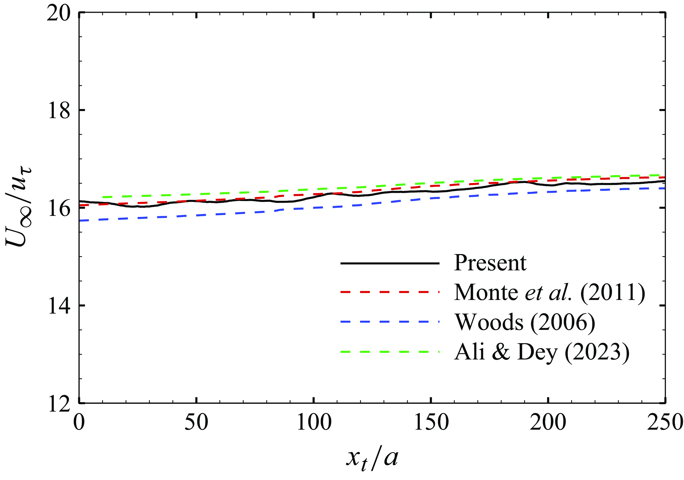
 $U_\infty /u_\tau$
against
 $x_t/a$
agrees well with the numerical results from Woods (2006), and the skin friction laws from Monte et al. (Reference Monte, Sagaut and Gomez2011) and Ali & Dey (Reference Ali and Dey2023), as shown in figure 3.
The streamwise distribution of the skin friction coefficient.

The streamwise distribution of
 $U_\infty /u_\tau$
in comparison with the prediction models: Monte et al. (Reference Monte, Sagaut and Gomez2011),
 $U_\infty /u_\tau =2.56\ln[Re_a\ln(1+\delta /a)]-2.53$
; Woods (2006),
 $U_\infty /u_\tau =2.97\ln[Re_a\ln(1+\delta /a)]-5.82$
; Ali & Dey (Reference Ali and Dey2023),
 $U_\infty /u_\tau =\sqrt { 2/[0.0456\,Re_a\ln(1+\delta /a)]^{-1/4} }$
.

The nominal thickness of the ATBL,
 $\delta$
, is determined by the wall-normal location of
 $U/U_\infty =0.99$
as in the TBL. The displacement thickness
 $\delta ^*$
and the momentum thickness
 $\theta$
are obtained by solving
 \begin{align}&\quad (\delta ^*+a)^2-a^2=2\int _{0}^{\delta }\left(1-\frac {U}{U_\infty }\right)(y+a){\rm d} {y}, \\[-10pt]\nonumber\end{align}
 \begin{align}& (\theta +a)^2-a^2=2\int _{0}^{\delta }\frac {U}{U_\infty }\left(1-\frac {U}{U_\infty }\right)(y+a){\rm d} {y}. \end{align}
Here,
 $U$
is the mean streamwise velocity, and
 $y=r-a$
is the distance to the wall of the cylinder. The boundary layer parameters at several streamwise locations are listed in table 1. In the present ATBL,
 $a^+$
is approximately 41, and
 $\delta /a$
varies from 7.25 to 13.08.
Boundary layer parameters; TBL data from Schlatter & Örlü (Reference Schlatter and Örlü2010).

The variations of (a)
 $\theta /a$
and (b)
 $H$
as functions of
 $\delta ^*/a$
. The fitting curves are (a)
 $\delta ^*/\theta =1.09$
and (b)
 $H=-0.047\ln(\delta ^*/a)+1.1022$
(Jordan Reference Jordan2014b
). The dashed line in (b) denotes the shape factor for TBL,
 $H=1.27$
.

The variations of the momentum thickness (
 $\theta /a$
) as a function of the displacement thickness (
 $\delta ^* /a$
) are shown in figure 4(a), in comparison with the experiments by Willmarth & Yang (Reference Willmarth and Yang1970), and numerical results by Woods (2006) and Jordan (Reference Jordan2014b
). The shape factor
 $H= \delta ^* / \theta$
is shown in figure 4(b). They all agree well with the fitting curve
 $H=-0.047\ln(\theta ^*/a)+1.1022$
given by Jordan (Reference Jordan2014b
), based on his simulations of the ATBL. It decreases as the ATBL develops, and is smaller than that of the TBL. This is mainly due to the curvature effect arising from the geometry of the ATBL. The present results agree well with those of Woods (2006), and are slightly higher than those of Jordan (Reference Jordan2014b
). For simplification, the shape factor can be considered as taking a constant value within a certain streamwise range (Jordan Reference Jordan2014b
), and then the integral expression of the skin friction coefficient
 $C_f$
can be obtained under the assumption
 ${\rm d}H/{\rm d}x=0$
. It can be written as (Kumar & Mahesh Reference Kumar and Mahesh2018)
 \begin{equation} C_f=\left (1+\frac {\theta }{a}\right )\frac {\rm {d}\delta ^*}{\rm {d} \textit {x}}\frac {2}{H}. \end{equation}
This expression has been employed for comparison in figure 2 as indicated by the blue open circles.
3.2. Mean velocity and Reynolds stresses
The mean velocity profile is compared to the former numerical and experimental results for the ATBL, as well as the TBL, in figure 5. The linear law and the log law proposed by Lueptow et al. (Reference Lueptow, Leehey and Stellinger1985) are also shown for comparison. Notably, although the ATBL cases in figure 5 cover a range
 $Re_a=580{-} 1450$
and a range of boundary layer thickness
 $\delta /a=5{-} 35$
, the mean velocity profiles collapse quite well with each other. Very near the wall with
 $y^+\lt 5$
, they still follow the linear law
 $U^+=y^+$
, just as in the TBL, indicating that at small values of
 $y^+/a^+$
, the curvature effect is not important (Neves et al. Reference Neves, Moin and Moser1994). According to Rao (Reference Rao1967), the effect of wall curvature would become manifest when
 $y^+\gt 20$
, and the profile will depart from the TBL, as confirmed in figure 5. At
 $y^+\gt 30$
, all the ATBL cases can be well predicted by the log law
 $U^+=(1/m)\ln y^+ +n$
, where according to Lueptow et al. (Reference Lueptow, Leehey and Stellinger1985), the parameters
 $1/m$
and
 $n$
take the values
 $1.5$
and
 $7.6$
, respectively. The large discrepancy between the log-region slopes of the ATBL and TBL implies the influence of the transverse curvature, which will be discussed in § 3.4.
Mean velocity profiles: present,
 $Re_a=670,\ \delta /a=12$
; Willmarth & Yang (Reference Willmarth and Yang1970),
 $Re_a=1439, \delta /a=27$
; Lueptow et al. (Reference Lueptow, Leehey and Stellinger1985),
 $Re_a=1510,\ \delta /a=34.5$
; Woods (2006),
 $Re_a=674,\ \delta /a=7.74$
; Jordan (Reference Jordan2014b
),
 $Re_a=586,\ \delta /a=4.4$
; Schlatter & Örlü (Reference Schlatter and Örlü2010),
 $Re_\delta =7780$
. Linear law,
 $U^+=y^+$
; log law,
 $U^+=1.5\ln y^++7.6$
(Lueptow et al. Reference Lueptow, Leehey and Stellinger1985).

Mean velocity profiles at different streamwise positions.

The mean velocity profiles at different streamwise positions are shown in figure 6. Near the wall
 $y^+\lt 10$
, all the profiles are in good agreement. The logarithmic region is getting higher, and the outer edge of boundary layer moves away from the wall as the boundary layer develops downstream. This suggests that the viscous units can well scale the near-wall region where the curvature effect is trivial, but away from the wall, there still lacks a universal scaling law.
The root mean squares of velocity fluctuations, together with the Reynolds shear stress, are shown in figure 7. The results are compared to the data of Neves et al. (Reference Neves, Moin and Moser1994) and Woods (2006) at similar
 $Re_a$
and
 $Re_\theta$
. The present results align well with the reference data in the near-wall region (
 $y^+\lt 50$
), and gradually deviate from them moving further away from the wall. Notably, the flows simulated by Neves et al. (Reference Neves, Moin and Moser1994) and Woods (2006) are statistically homogeneous in the streamwise direction, and are not capable of providing reliable representation of the outer regions of the boundary layer (Neves et al. Reference Neves, Moin and Moser1994).
Wall-normal distribution of root mean squares of velocity fluctuations and Reynolds shear stress: (a)
 $u_{rms}^{\prime +}$
, (b)
 $v_{rms}^{\prime +}$
, (c)
 $w_{rms}^{\prime +}$
, (d)
 $-\langle {u'v'} \rangle ^+$
. In (d), present,
 $Re_a=670$
,
 $Re_\theta =950$
; Woods (2006),
 $Re_a=674$
,
 $Re_\theta =803$
; Neves et al. (Reference Neves, Moin and Moser1994),
 $Re_a=674$
,
 $Re_\theta =500$
.

Wall-normal distribution of root mean squares of velocity fluctuations and Reynolds shear stress. Original: (a)
 $u_{rms}^{\prime +}$
, (b)
 $v_{rms}^{\prime +}$
, (c)
 $w_{rms}^{\prime +}$
, (d)
 $-\langle {u'v'} \rangle ^+$
. TBL: Schlatter & Örlü (Reference Schlatter and Örlü2010).

Figure 8 shows the wall-normal distributions of the root mean squares of velocity fluctuations and Reynolds shear stress at three different streamwise locations in the present ATBL in comparison with those in the TBL of Schlatter & Örlü (Reference Schlatter and Örlü2010). It is obvious that turbulence in the present ATBL is much weaker than that in the TBL at similar
 $Re_\tau$
. It is known that the Reynolds shear stress and turbulent intensities increase as the boundary layer develops downstream with increasing
 $Re_\tau$
in the TBL. However, in the current TBL over a slender cylinder, our observations reveal a slight decreasing trend of the turbulent fluctuations of the radial and circumferential components. It is worth noting that the curvature parameter
 $\delta /a$
of the ATBL increases during its streamwise development, whereas an increase in the curvature parameter leads to a decrease in the turbulent intensities and Reynolds shear stress (Neves et al. Reference Neves, Moin and Moser1994; Woods 2006). Therefore, in the development of the ATBL, the effect of increasing friction Reynolds number and the effect of increasing curvature are competitively related. According to Neves et al. (Reference Neves, Moin and Moser1994) and Woods (2006), the influence of curvature is stronger at low Reynolds numbers (
 $Re_\tau =200{-} 600$
). It could therefore be inferred that in the present ATBL, the effect of curvature prevails for both radial (figure 8
b) and circumferential (figure 8
c) turbulent intensities.
3.3. Budget of the Reynolds stress transport
The transport equations for Reynolds stresses can be written as
 \begin{eqnarray} \frac {{\rm D}{\langle {u_i^{\prime}u_{\!j}^{\prime}} \rangle }}{\rm {D} \mathit{t}}&=&P_{\textit{ij}}+D_{\textit{ij}}^\nu +D_{\textit{ij}}^T+\varPi _{\textit{ij}}+\epsilon _{\textit{ij}}, \end{eqnarray}
where
 $P_{\textit{ij}}$
represents the production term,
 $D_{\textit{ij}}^\nu$
and
 $D_{\textit{ij}}^T$
are the viscous and turbulent diffusion terms,
 $\varPi _{\textit{ij}}$
is the velocity–pressure-gradient term, and
 $\epsilon _{\textit{ij}}$
is the dissipation term. Correspondingly, the transport equation for the turbulent kinetic energy
 $k= \langle {u_i^{\prime}u_i^{\prime}} \rangle /2$
can be written as
 \begin{eqnarray} \frac {\rm {D}\mathit{k}}{\rm {D} \mathit{t}}&=&P_{k}+D_{k}^\nu +D_k^T+\varPi _{k}+\epsilon _{k}. \end{eqnarray}
The detailed expressions for each term in cylindrical coordinates are given in Appendix A.
Figure 9(a) shows the budget of turbulent kinetic energy transport equation in the present ATBL at
 $Re_\theta =999$
, together with that in the TBL of Schlatter & Örlü (Reference Schlatter and Örlü2010) at
 $Re_\theta =1006$
. The convective term and velocity–pressure-gradient term are both negligible compared with other terms in the whole range of the boundary layer. Very near the wall with
 $y^+\lt 3$
, the viscous diffusion balances the viscous dissipation effect. The production term and the tubulent diffusion term become important, and balance with the two viscous terms in the range
 $3\lt y^+\lt 50$
. Further away from the wall, the balance is between the production and dissipation terms. The viscous diffusion term is positive within
 $y^+\lt 4$
and becomes negative at
 $y^+\gt 4$
, while the turbulent diffusion term changes sign a little further away from the wall at
 $y^+=7$
. Compared with the TBL, the transverse curvature in the present ATBL weakens all the terms in the transport equation of
 $k$
. Despite the discrepancy in the magnitudes, it is interesting to note that the zero-crossing wall-normal positions of the viscous diffusion and turbulent diffusion terms are almost the same for both flat wall and curved wall cases, and similarly for the peak position of the production term. Therefore, each budget term was rescaled by the respective dissipation rate at the wall for the present ATBL and TBL, as displayed in figure 9(b). The rescaling makes the terms of the present ATBL collapse well with those of the TBL, especially in the viscous sublayer. This suggests a similar mechanism in the transport of turbulent kinetic energy. However, notably, away from the wall, the production and dissipation terms in the present ATBL are both weaker than those in the TBL.
Budget of the transport equation for turbulent kinetic energy scaled by (a)
 $u^4_\tau /\nu$
and (b) the dissipation rate
 $\epsilon _k$
at the wall. Solid line, present results,
 $Re_\theta =999$
; dashed line, TBL results of Schlatter & Örlü (Reference Schlatter and Örlü2010),
 $Re_\theta =1006$
. Red,
 $P_k$
; black,
 $D^\nu _k$
; blue,
 $D^T_k$
; orange,
 $\epsilon _k$
; green,
 $\varPi _k$
; magenta,
 $(V\,\partial k/\partial y+U\,\partial k/\partial x)$
.

Figure 10(a–d) show the budgets of Reynolds stress transport equations in comparison with the TBL results by Schlatter & Örlü (Reference Schlatter and Örlü2010). All the terms are also normalised by the dissipation rate
 $\epsilon _k$
at the wall. In general, the transport of streamwise turbulent kinetic energy
 $ \langle {u'u'} \rangle$
is similar between the present and flat plate cases under the rescaling, as shown in figure 10(a). However, the transport of the wall-normal and spanwise turbulent kinetic energy, as well as the Reynolds shear stress, is still much weaker in the ATBL compared with the TBL.
Figure 10(b) shows the budget of the transport equation of
 $ \langle {v'v'} \rangle$
. In the wall-normal direction, the production term is nearly zero and the energy comes from the streamwise direction via the redistribution of the pressure–strain-rate term. Near the wall within
 $y^+\lt 10$
, the turbulent diffusion
 $D_{rr}^{T}$
and velocity–pressure-gradient
 $\varPi _{rr}$
terms are both slightly negative, and together with the dissipation term
 $\epsilon _{rr}$
balance the viscous diffusion term
 $D_{rr}^\nu$
. Away from the wall when
 $y^+\gt 10$
, viscous diffusion becomes negligible, and the main contributor is the pressure term
 $\varPi _{rr}$
, which is balanced by turbulent diffusion
 $D_{rr}^T$
and viscous dissipation
 $\epsilon _{rr}$
. When
 $y^+\gt 100$
, turbulent diffusion becomes unimportant; the balance is only between
 $\varPi _{rr}$
and
 $\epsilon _{rr}$
. Compared with the TBL case, the pressure term and dissipation term are remarkably reduced in the present ATBL, while the turbulent diffusion term has magnitude similar to that in the flat plate case, and is even larger than the dissipation term in
 $30\lt y^+\lt 80$
. In figure 10(c), the budget of the
 $\langle {w'w'} \rangle$
transport equation is displayed. The production term is zero, and the energy in the circumferential direction also comes from the streamwise direction via pressure term
 $\varPi _{\theta \theta }$
. Near the wall within
 $y^+\lt 3$
, turbulent diffusion
 $D_{\theta \theta }^T$
is negligible; it is viscous diffusion
 $D_{\theta \theta }^\nu$
and pressure term
 $\varPi _{\theta \theta }$
that balance the dissipation
 $\epsilon _{\theta \theta }$
. Also,
 $D_{\theta \theta }^\nu$
becomes negative when
 $y^+\gt 3$
, and has magnitude similar to that of
 $D_{\theta \theta }^T$
. They both become negligible when
 $y^+\gt 50$
, where the pressure term is balanced only by the dissipation term. Compared with the TBL, the pressure and dissipation terms are obviously reduced in the present ATBL, while the change in the diffusion terms is insignificant away from the wall. Figure 10(a) shows the budget of the
 $ \langle {u'u'} \rangle$
transport equation, which is similar to that of the turbulent kinetic energy
 $k$
. Only two points need to be addressed. The first point is that the viscous diffusion
 $D_{xx}^\nu$
and dissipation
 $\epsilon _{xx}$
in
 $y^+\lt 3$
in the present case are larger than those in the TBL, which is in accordance with the reduced magnitude of
 $D_{\theta \theta }^\nu$
and
 $\epsilon _{\theta \theta }$
. The second point is that the pressure term
 $\varPi _{xx}$
is negative in the whole channel, suggesting that the energy is transferred from the streamwise direction to the wall-normal and circumferential directions. Notably, its magnitude is much less than that in the TBL, indicating the hindrance of the inter-component transfer of turbulent kinetic energy due to the transverse curvature.
Budget of the transport equations for (a)
 $\langle {u' u'} \rangle$
, (b)
 $\langle {v' v'} \rangle$
, (c)
 $\langle {w' w'} \rangle$
, (d)
 $-\langle {u'v'} \rangle$
. Solid line, present ATBL results,
 $Re_\theta =999$
; dashed line, TBL results of Schlatter & Örlü (Reference Schlatter and Örlü2010),
 $Re_\theta =1006$
. Red,
 $P_{\textit{ij}}$
; black,
 $D^\nu _{\textit{ij}}$
; blue,
 $D^T_{\textit{ij}}$
; orange,
 $\epsilon _{\textit{ij}}$
; green,
 $\varPi _{\textit{ij}}$
.

Figure 10(d) shows the budget of the Reynolds shear stress
 $- \langle {u'v'} \rangle$
transport equation. In the near-wall region with
 $y^+\lt 10$
, the viscous and turbulent diffusion terms are positive, and together with the production term, balance the velocity–pressure-gradient term and dissipation term. When
 $y^+\gt 10$
, the dissipation and viscous diffusion terms tend to zero, and the turbulent diffusion term becomes negative. The turbulent diffusion term together with the pressure term balance with the production term. Compared with the TBL case, the production and pressure terms are greatly reduced in the present ATBL.
The above analysis on the Reynolds stress transport suggests that the transverse curvature in the ATBL hinders the inter-component energy transfer by reducing the pressure–velocity-gradient terms especially when
 $y^+\gt 10$
. In radial and circumferential directions, there is no production of turbulent kinetic energy from the mean shear, and the pressure terms act as the main contributors. Therefore, the radial component of turbulent intensity is suppressed, which causes the attenuation of the production term of Reynolds shear stress. The weakened Reynolds shear stress further reduces the production of turbulent kinetic energy, as shown in figure 9(a).
3.4. Curvature-weighted transformation
The above discussions show that when normalised by wall friction velocity as in the TBL, the mean velocity profile, Reynolds stresses and turbulence production in the ATBL all manifest clear curvature effects. In the following, we try to propose a curvature-weighted transformation to collapse the TBL and ATBL results together. First, the mean momentum balance in the streamwise direction in the ATBL is compared to that in the TBL, as Neves et al. (Reference Neves, Moin and Moser1994) did for the pressure-driven flows. In the TBL and ATBL, the total shear stress satisfies
 \begin{equation} \nu \frac {{\partial U}}{{\partial y}} - \langle {u'v'} \rangle = \frac {{{\tau _w}}}{\rho } + UV{\rm { + }}\frac {\partial }{{\partial x}}\int _0^y {( {UU} )\,{\rm {d}}\xi } \end{equation}
and
 \begin{equation} \nu \frac {{\partial U}}{{\partial r}} - \langle {u'v'} \rangle = \frac {a}{r}\frac {{{\tau _w}}}{\rho } + UV + \frac {\partial }{{\partial x}}\int _0^y {\left ( {\frac {{a + \xi }}{{a + y}}UU} \right )} {\rm {d}}\xi, \end{equation}
respectively. Near the wall, if the contribution of the convection terms is neglected, then the constant stress assumption is recovered in the TBL as
 \begin{equation} \nu \frac {{\partial U}}{{\partial y}} - \langle {u'v'} \rangle = \frac {{{\tau _w}}}{\rho }, \end{equation}
while the corresponding expression in the ATBL is
 \begin{equation} \nu \frac {{\partial U}}{{\partial r}} - \langle {u'v'} \rangle = \frac {a}{r}\frac {{{\tau _w}}}{\rho }. \end{equation}
In the TBL, the velocity scale is
 ${u_\tau } = \sqrt {{\tau _w}/\rho }$
, and it is clear that for the ATBL, the corresponding velocity scale should be
 $u_\tau \sqrt {a/r}=u_\tau \sqrt {1/(1+\kappa y)}\equiv u_{\tau a}$
, where
 $\kappa =1/a$
is the curvature of the cylinder surface. In the flat wall case,
 $\kappa =0$
and
 $u_{\tau a}=u_\tau$
. Normalised by
 $u_\tau$
and
 $u_{\tau a}$
, (3.8) and (3.9) could be rewritten as
 \begin{equation} \frac {{\partial {U^{\rm { + }}}}}{{\partial {y^{\rm { + }}}}} - \langle {{{u'}^{\rm { + }}}{{v'}^{\rm { + }}}} \rangle = 1 \end{equation}
and
 \begin{equation} \frac {r}{a}\frac {{\partial {U^ + }}}{{\partial {y^ + }}} - \langle {{{u'}^*}{{v'}^*}} \rangle = {{1}}. \end{equation}
Here the superscripts ‘+’ and ‘*’ represent the normalisation by
 $u_\tau$
and
 $u_{\tau a}$
, respectively. The above relations suggest that the mean shear in the ATBL weighted by
 $r/a$
can be analogised to the mean shear in the TBL, and the characteristic velocity scale for velocity fluctuations in the ATBL is
 $ u_{\tau a}$
rather than
 $u_\tau$
in the near-wall region.
To validate the above analysis, we first calculated the curvature-weighted mean shear of the TBL as a prediction for the mean shear of the ATBL:
 \begin{equation} \left (\frac {\partial U^+}{\partial y^+}\right )_{\!\textit{ATBL}} =\frac {1}{1+\kappa ^+ y^+}\left (\frac {\partial U^+}{\partial y^+}\right )_{\!\textit{TBL}}\!. \end{equation}
The predicted mean shear is compared with that of the present ATBL in figure 11(a). It is clear that using the mean shear of the TBL and the curvature-weighted transformation, the mean shear of the ATBL can be well predicted. This transformation can be further applied to the mean velocity. The mean velocity of ATBL can be predicted from that of the TBL by
 \begin{equation} U_{\textit{ATBL}}^+(y^+)=\int _0^{y^+}\!\!\frac {1}{1+\kappa ^+ \xi ^+}\left (\frac {\partial U^+}{\partial \xi ^+}\right )_{\!\textit{TBL}}\rm {d}\xi ^+. \end{equation}
The predicted mean velocity profile is compared with that of the present ATBL in figure 11(b). The great discrepancy between the TBL and the ATBL above the buffer layer is effectively alleviated by the transformation.
Distributions of (a) mean shear and (b) mean streamwise velocity. TBL,
 $Re_\theta =1006$
from Schlatter & Örlü (Reference Schlatter and Örlü2010); ATBL, present data at
 $Re_\theta =999$
; predicted ATBL, given by (3.12) in (a) and (3.13) in (b).

The Reynolds stresses of the ATBL can also be predicted by those of the TBL and the curvature-weighted transformation. According to (3.10) and (3.11), the predicted Reynolds shear stress and root mean square of velocity fluctuations can be written as
 \begin{equation} \langle {u'v'} \rangle _{\textit{ATBL}}^+ =\frac {1}{1+\kappa ^+ y^+}\langle {u'v'} \rangle _{\textit{TBL}}^+ \end{equation}
and
 \begin{equation} \big(u^{\prime +}_{i,rms} \big)_{\textit{ATBL}} =\sqrt {\frac {1}{1+\kappa ^+ y^+}}\big(u^{\prime +}_{i,rms} \big)_{\textit{TBL}}, \end{equation}
respectively. The predicted results are compared with the present ATBL results in figure 12(a–d). The wide difference between the ATBL and TBL results is effectively alleviated. Especially for the streamwise fluctuation and Reynolds shear stress, the data are collapsed quite well in the near-wall region. In addition, the outer region of the ATBL seems to have a wake-like flow regime (Lueptow et al. Reference Lueptow, Leehey and Stellinger1985), thus may not be explained by considering only the curvature information
 $r/a$
. The effective scaling of turbulent fluctuation intensities by applying the curvature-weighting operation suggests a certain degree of similarity between the ATBL and TBL.
Distributions of the root mean squares of velocity fluctuations and Reynolds shear stress: (a)
 $u_{rms}^{\prime +}$
, (b)
 $v_{rms}^{\prime +}$
, (c)
 $w_{rms}^{\prime +}$
, (d)
 $-\langle {u'v'}^+ \rangle$
. TBL,
 $Re_\theta =1006$
from Schlatter & Örlü (Reference Schlatter and Örlü2010); ATBL, present data at
 $Re_\theta =999$
; predicted ATBL, given by (3.15) in (a–c) and (3.14) in (d).

Considering the similarity in Reynolds stresses and mean velocity profile under the curvature-weighted transformation, we further applied the prediction to the production term of turbulent kinetic energy in (A5), which is dominated by
 $-\langle {u'v'} \rangle\, \partial U / \partial r$
. According to (3.12) and (3.14), the predicted production term of turbulent kinetic energy can be expressed as
 \begin{equation} \left(P_k^+\right)_{\textit{ATBL}} =\frac {1}{(1+\kappa ^+ y^+)^2}\left(P_k^+\right)_{\textit{TBL}}\!. \end{equation}
Figure 13 shows the predicted production term, and the good agreement with the present ATBL result further confirms the reliability of the curvature-weighted transformation.
Distributions of the production terms of turbulent kinetic energy. TBL,
 $Re_\theta =1006$
from Schlatter & Örlü (Reference Schlatter and Örlü2010); ATBL, present data at
 $Re_\theta =999$
; predicted ATBL, given by (3.16).

Contours of streamwise velocity fluctuation on a cylindrical surface at (a)
 $y^+=0.5$
, (b)
 $y^+=5$
, (c)
 $y^+=15$
, (d)
 $y^+=30$
, with contour levels from
 $-2u_{rms}(y^+)$
to
 $2u_{rms}(y^+)$
. The streamwise length of the domain displayed is
 $174a$
. Blue,
 $u'\lt 0$
; red,
 $u'\gt 0$
.

4. Turbulence coherent structures
The coherent structures have been investigated thoroughly in the flat plate TBL (Robinson Reference Robinson1991). However, we lack a comprehensive description and examination of coherent structures within the TBLs over a slender cylinder. The numerical results reveal that a slender cylinder could support a boundary layer that is exceptionally thicker compared to its own radius
 $a$
, as shown in table 1, within which there exist abundant coherent structures. In the following, the velocity streaks and vortical structures in the present ATBL under the influence of transverse curvature will be analysed.
Figure 14 shows the instantaneous distributions of streamwise velocity fluctuation on the
 $x{-}r\theta$
planes at different radial positions corresponding to
 $y^+=0.5,5,15,30$
. Two or three low-speed streaks can be clearly observed, and the streamwise positions of the streaks are in good accordance in the four different planes. The high coherence of velocity streaks at different
 $y^+$
can be further evidenced by the iso-contours of
 $u'$
on the cross-planes at different streamwise positions, as shown in figure 15. It is clear that the streak meanders in the circumferential direction as it develops downstream, and keeps good accordance below
 $y^+=30$
. Notably, within the circumferential span of the cylinder, three low-speed streaks are most frequently observed at different streamwise locations within
 $y^+\lt 30$
.
Getting away from the wall, as shown in figure 14(a–d), the circumferential spacing of low-speed streaks increases. Considering that the number of streaks in a circumference stays the same at different radial positions, the mean circumferential spacing of streaks at different
 $y^+$
could be estimated by
 $\lambda _\theta ^+=2\unicode{x03C0} r^+/n$
, where
 $n$
is the number of streaks, and
 $r^+=a^++y^+$
. In the present simulated flow,
 $n=3$
,
 $a^+=41$
, thus it is easy to get
 $\lambda _\theta ^+=87, 96, 117,149$
at
 $y^+=0.5, 5, 15,30$
, respectively. The mean circumferential spacing of velocity streaks can also be quantified by the autocorrelation coefficient of streamwise velocity fluctuations in the circumferential direction, as shown in figure 16. The negative minimum is reached for
 $r^+\,\Delta \theta = 44, 47, 61,84$
at
 $y^+=0.5, 5, 15,30$
, respectively. Therefore, the mean spacing of the streaks, which equals twice the separation at which the coefficient reaches a minimum, is
 $88, 94, 122,168$
. This is consistent with the estimation based on
 $r^+$
and
 $n$
. Notably, in the flat wall case, the mean spanwise spacing of low-speed streaks is nearly constant, with value
 $\lambda _z^+ = 110$
in the near-wall region
 $y^+\lt 10$
, and increases with distance from the wall for
 $y^+ \gt 10$
(Kim, Moin & Moser Reference Kim, Moin and Moser1987; Lagraa, Labraga & Mazouz Reference Lagraa, Labraga and Mazouz2004). It reaches a value
 $\lambda _z^+\approx145$
at
 $y^+=30$
(Smith & Metzler Reference Smith and Metzler1983; Lagraa et al. Reference Lagraa, Labraga and Mazouz2004). Compared with the flat wall case, in the present flow along a cylindrical wall, the streak spacing in the near-wall region is smaller and increases faster with the distance from the wall. This is mainly due to the variation of the circumferential span of the flow field at different radial positions.
Instantaneous distribution of
 $u^{\prime +}$
on the cross-planes at (a)
 $x_t^+=1645$
, (b)
 $x_t^+=3620$
and (c)
 $x_t^+=5050$
. The black dashed cycle indicates
 $y^+=30$
.

Autocorrelation coefficient of streamwise velocity fluctuations in the circumferential direction at different radial positions.

The velocity streaks are the footprints of the near-wall quasi-streamwise vortices. Figure 17 shows the distribution of the low-speed streaks and vortex structures within
 $y^+\lt 40$
. A large number of quasi-streamwise vortices are located near the meandering streaks in the near-wall region. Typically, both positive (red) and negative (green) streamwise vortices tend to appear near the turnings of meandering streaks with
 $\partial u'/\partial x\gt 0$
, indicating that the stretching mechanism is still significant in the generation of streamwise vortices in the ATBL as that in the TBL (Schoppa & Hussain Reference Schoppa and Hussain2002).
Distribution of velocity streaks and vortical structures within
 $y^+\lt 40$
. Blue, iso-surfaces of
 $u^{\prime +}=-2.5$
; red, iso-surfaces of
 $Q(\delta /U_\infty )^2=2.2$
with
 $\omega _x^{\prime}\gt 0$
; green, iso-surfaces of
 $Q(\delta /U_\infty )^2=2.2$
with
 $\omega _x^{\prime}\lt 0$
.

Iso-surfaces of
 $Q(\delta /U_\infty )^2=0.87$
in the region of (a)
 $y^+\lt 40$
dyed by
 $\omega _x^{\prime}$
, (b)
 $40\leqslant y^+\leqslant 160$
dyed by
 $\omega _r^{\prime}$
, (c)
 $y^+\gt 160$
dyed by
 $\omega _\theta^{\prime}$
.

In the TBL, the quasi-streamwise vortices prevalent in the near-wall region are considered as leg parts of the hairpin-like vortical structures, and away from the wall, the neck parts with larger wall-normal vorticity, and head parts with larger spanwise vorticity, will gradually become dominant (Robinson Reference Robinson1991). In the present ATBL, the vortical structures in different wall-normal regions are first considered. Figure 18 shows the vortical structures by the iso-surfaces of
 $Q$
, the second invariant of the velocity gradient tensor, in the regions
 $y^+\lt 40$
,
 $40\leqslant y^+\leqslant 160$
and
 $y^+\gt 160$
, respectively. As shown in figure 18(a), the near-wall region (
 $y^+\lt 40$
) is dominated by quasi-streamwise vortices with strong
 $\omega _x^{\prime}$
, which experience downstream lifting up and circumferential tilting. In the region
 $40\leqslant y^+\leqslant 160$
shown in figure 18(b), the vortical structures mostly tend to align in the wall-normal direction with strong
 $\omega _r^{\prime}$
. Beyond
 $y^+\gt 160$
, as displayed in figure 18(c), arch-like structures with negative circumferential vorticity become prevalent, indicating the dominance of the prograde vortices over the retrograde vortices as in the TBL.
In the outer region of the ATBL, hairpin vortices tend to grow and migrate as hairpin vortex packets similar with those in the TBL (Adrian Reference Adrian2007). Figure 19 shows an example of hairpin vortex packet. The heads of hairpin vortices are located along the contour line
 $u=0.87U_\infty$
, forming a ramp-like shape similar to that of the TBL (Adrian, Meinhart & Tomkins Reference Adrian, Meinhart and Tomkins2000), as shown in figure 19(a). Figure 19(b) clearly shows that the hairpin vortex packet consists of
 $5{-}6$
single hairpin vortices coherently distributed along the constant streamwise velocity line in different streamwise and radial positions. Moreover, the packet consists of several hairpin vortices downstream, labelled F–H in figure 19, with almost the same convection velocity, which possibly are secondary structures induced by the adjacent vortices. They align in the streamwise direction coherently with the upstream structures, and together create a larger zone of nearly uniform streamwise momentum. The large-scale hairpin packet occupies approximately 1400 wall units in the streamwise direction, and reaches up to
 $y^+=200$
in the radial direction in figure 19. In addition, the hairpin vortices between A and B, influenced by the large curvature, align in different circumferential directions and thus are not captured in the
 $x{-}r$
plane in figure 19(a). This indicates that the hairpin packets could grow around the cylinder under the curvature effect.
Illustrative example of hairpin vortex packets. (a) Instantaneous velocity vectors in the
 $x{-}y$
plane viewed in a frame moving at
 $U_c=0.88U_\infty$
. The black solid lines are contours of
 $u=0.87U_\infty$
and
 $0.35U_\infty$
. Labels A–H indicate the heads of hairpin vortices identified by
 $Q(\delta /U_\infty )^2\gt 5$
and
 $\omega _\theta \delta /U_\infty \lt -5$
. (b) Hairpin vortex packet identified by the iso-surfaces
 $Q(\delta /U_\infty )^2=5$
.

5. Conclusions
In the present study, DNS are performed for an ATBL along a slender cylinder. The transition of laminar inflow is triggered by wall blowing and suction, and a fringe region is adopted to use a periodic condition in the streamwise direction. In the developed turbulent region, the cylinder radius is approximately 41 viscous units, the boundary layer thickness varies from 7 to 13 times the cylinder radius, and the friction Reynolds number is in the range 300–510. The simulation is validated by comparing the streamwise distribution of the skin friction coefficient and boundary layer thickness, as well as the wall-normal distribution of mean velocity and Reynolds stresses, with existing experimental and numerical results. Turbulence statistics and coherent structures are further compared with those of the TBL to reveal the influence of the transverse curvature.
The curvature effects are first discussed under the normalisation using wall friction velocity. For both the ATBL and the TBL, the mean velocity profiles obey the linear law when
 $y^+\lt 5$
. The wall curvature manifests its effect until
 $y^+=20$
, around which the ATBL profiles start to deviate from the TBL profile. At
 $y^+\gt 30$
, the ATBL profiles also follow the log law but with a much smaller slope, approximately 1.5, in comparison with the slope approximately 2.5 in the TBL. The turbulence intensities and Reynolds shear stress in the ATBL are much weaker than those in the TBL within
 $y^+\lt 300$
, as are the terms in the transport equation of turbulent kinetic energy.
To reveal the mechanism for turbulence suppression under the influence of transverse curvature, the budgets of Reynolds stress transport equations are analysed. When scaling all the budget terms by their respective dissipation rates at the wall, it is clear that the pressure terms, which act as the contributors for the velocity fluctuations in wall-normal and spanwise directions, are much weaker in the ATBL than in the TBL. The spanwise curvature hinders the inter-component energy transfer, reduces the wall-normal Reynolds stress, and sequentially results in the weakened production term of Reynolds shear stress and turbulent kinetic energy.
To compensate for the curvature effects on mean velocity and Reynolds stresses, a curvature-weighted transformation is proposed. It is based on the analogy of total shear stress relations between the ATBL and the TBL. It is suggested that the mean shear weighted by the wall curvature
 $(1+\kappa ^+ y^+)(\partial U^+/\partial y^+)$
in the ATBL is equivalent to the mean shear
 $\partial U^+/\partial y^+$
in the TBL, so does the Reynolds shear stress. Based on this analogy, the mean velocity and Reynolds stresses in the ATBL can be well constructed using the TBL counterparts and curvature-weighted transformation.
Velocity streaks and vortical structures are also prevalent in the ATBL as in the TBL. The curvature effect is manifested in the mean circumferential spacing of low-speed streaks. The number of streaks in a circumference at different wall-normal locations is unchanged when
 $y^+\lt 30$
, therefore the mean streak spacing increases linearly with
 $y^+$
in the near-wall region. This is different from the TBL, in which the mean spanwise spacing of streaks is nearly constant, with value approximately 110 wall units in the near-wall region
 $y^+\lt 10$
. The near-wall region with
 $y^+\lt 40$
is dominated by quasi-streamwise vortices, and the arch-like vortices are common in the outer region. They can be considered as building blocks of hairpin-like vortical structures as in the TBL. There exist hairpin vortex packets in the outer region of the boundary layer, which could reach up to
 $y^+=200$
in the radial direction. They are prevalent in the logarithmic region, and grow in both the circumferential and streamwise directions under the curvature effect.
Funding
This work is supported by the National Natural Science Foundation of China under grant nos 92252204, 12425206 and 12388101.
Declaration of interests
The authors report no conflict of interest.
Appendix A
The detailed expressions for each term of the transport equations of Reynolds stresses are written as follows:
 \begin{eqnarray} P_{rr}& = & -\langle {v'v'} \rangle \frac {\partial V}{\partial r}-\langle {u'v'} \rangle \frac {\partial V}{\partial x}, \nonumber \\ D_{rr} & = & \frac {1}{2}\frac {\partial }{\partial r} \left ( {-\langle {v'v'v'} \rangle +\nu \frac {\partial \langle {v'v'} \rangle }{\partial r}} \right ) +\frac {1}{2} \frac {\partial }{\partial x} \left ( {-\langle {u'v'v'} \rangle +\nu \frac {\partial \langle {v'v'} \rangle }{\partial x}} \right ) \quad \nonumber \\ && \mbox{} - \frac {1}{2}\frac {\langle {v'v'v'}\rangle }{r}+\frac {1}{2}\frac {\langle {v'w'w'}\rangle }{r}+\nu \frac {1}{2r}\frac {\partial \langle {v'v'} \rangle }{\partial r}, \nonumber \\ \varPi _{rr} & = & \frac {1}{\rho } \left ( \bigg\langle {p'\frac {\partial v'}{\partial r}} \bigg\rangle - \frac {\partial }{\partial r} \langle {v'p'} \rangle \right )\!, \nonumber \\ \epsilon _{rr} & = & -\nu \left ( {\bigg\langle {\frac {\partial v'}{\partial r} \frac {\partial v'}{\partial r}} \bigg\rangle +\bigg\langle {\frac {\partial v'}{\partial x} \frac {\partial v'}{\partial x}} \bigg\rangle +\frac {1}{r^2}\bigg\langle {\frac {\partial v'}{\partial \theta } \frac {\partial v'}{\partial \theta }} \bigg\rangle } \right ) \quad \nonumber \\ && \mbox{} -\nu \frac {\langle {v'v'} \rangle }{2r^2}-\nu \bigg\langle { \frac {2v'}{r^2} \frac {\partial w'}{\partial \theta } }\bigg\rangle, \end{eqnarray}
 \begin{eqnarray} P_{\theta \theta }& = & -\frac {V \langle {w'w'}\rangle }{r}, \quad \nonumber \\ D_{\theta \theta } & = & \frac {1}{2}\frac {\partial }{\partial r} \left ( -\langle {v'w'w'} \rangle +\nu \frac {\partial \langle {w'w'} \rangle }{\partial r} \right )+ \frac {1}{2} \frac {\partial }{\partial x} \left ( {-\langle {u'w'w'} \rangle +\nu \frac {\partial \langle {w'w'} \rangle }{\partial x}} \right ) \quad \nonumber \\ && \mbox{} +\nu \frac {1}{2r} \frac {\partial \langle {w'w'} \rangle }{\partial r}- \frac {3\langle {v'w'w'}\rangle }{2r}, \quad \nonumber \\ \varPi _{\theta \theta } & = & \frac {1}{r\rho } \bigg\langle {p'\frac {\partial w'}{\partial \theta }} \bigg\rangle, \quad \nonumber \\ \epsilon _{\theta \theta } & = & -\nu \left ( {\bigg\langle {\frac {\partial w'}{\partial r} \frac {\partial w'}{\partial r}} \bigg\rangle +\bigg\langle {\frac {\partial w'}{\partial x} \frac {\partial w'}{\partial x}} \bigg\rangle +\frac {1}{r^2}\bigg\langle {\frac {\partial w'}{\partial \theta } \frac {\partial w'}{\partial \theta }} \bigg\rangle } \right ) \quad \nonumber \\ && \mbox{} -\nu \frac {w'w'}{r^2}+\nu \bigg\langle {\frac {2w'}{r^2}\frac {\partial v'}{\partial \theta }}\bigg\rangle,\end{eqnarray}
 \begin{eqnarray} P_{xx}& = & -\langle {u'v'} \rangle \frac {\partial U}{\partial r}-\langle {u'u'} \rangle \frac {\partial U}{\partial x}, \quad \nonumber \\ D_{xx} & = & \frac {1}{2}\frac {\partial }{\partial r} \left ( -\langle {v'u'u'} \rangle + \nu \frac {\partial \langle {u'u'} \rangle }{\partial r} \right )+\frac {1}{2} \frac {\partial }{\partial x} \left ( {-\langle {u'u'u'} \rangle +\nu \frac {\partial \langle {u'u'} \rangle }{\partial x}} \right ) \quad \nonumber \\ && \mbox{} +\frac {\nu }{2r}\frac {\partial \langle {u'u'} \rangle }{\partial r}-\frac {\langle {v'u'u'}\rangle }{2r}, \quad \nonumber \\ \varPi _{xx} & = & \frac {1}{\rho } \left ( \bigg\langle {p'\frac {\partial u'}{\partial x}} - \frac {\partial }{\partial x} \langle {p'u'} \rangle \bigg\rangle \right )\!, \quad \nonumber \\ \epsilon _{\theta \theta } & = & -\nu \left ( {\bigg\langle {\frac {\partial u'}{\partial r} \frac {\partial u'}{\partial r}} \bigg\rangle +\bigg\langle {\frac {\partial u'}{\partial x} \frac {\partial u'}{\partial x}} \bigg\rangle +\frac {1}{r^2}\bigg\langle {\frac {\partial u'}{\partial \theta } \frac {\partial u'}{\partial \theta }} \bigg\rangle } \right )\!, \end{eqnarray}
 \begin{eqnarray} P_{xr} & = & -\langle {u'v'} \rangle \frac {\partial V}{\partial r}-\langle {v'v'} \rangle \frac {\partial U}{\partial r}-\langle {u'u'} \rangle \frac {\partial V}{\partial x}-\langle {u'v'} \rangle \frac {\partial U}{\partial x }, \quad \nonumber \\ D_{xr} & = & \frac {\partial }{\partial r} \left ( {-\langle {u'v'v'} \rangle +\nu \frac {\partial \langle {u'v'} \rangle }{\partial r}} \right ) \quad \nonumber \\ && \mbox{} +\frac {\partial }{\partial x} \left ( {-\langle {v'u'u'} \rangle +\nu \frac {\partial \langle {u'v'} \rangle }{\partial x}} \right ) \quad \nonumber \\ && \mbox{} +\frac {\nu }{r} \frac {\partial \langle {u'v'} \rangle }{\partial r}-\frac {\langle {u'v'v'}\rangle }{r}+\frac {\langle {u'w'w'}\rangle }{r}, \quad \nonumber \\ \varPi _{xr} & = & \frac {1}{\rho } \langle {p'\left ( {\frac {\partial u'}{\partial r}+\frac {\partial v'}{\partial x} } \right ) } \rangle -\frac {1}{\rho } \left ( \frac {\partial }{\partial r} \langle {p'u'} \rangle +\frac {\partial }{\partial x} \langle {p'v'} \rangle \right )\!, \quad \nonumber \\ \epsilon _{xr} & = & -2\nu \left ( {\bigg\langle {\frac {\partial u'}{\partial r} \frac {\partial v'}{\partial r}} \bigg\rangle +\bigg\langle {\frac {\partial u'}{\partial x} \frac {\partial v'}{\partial x}} \bigg\rangle +\frac {1}{r^2}\bigg\langle {\frac {\partial u'}{\partial \theta } \frac {\partial v'}{\partial \theta }} \bigg\rangle } \right ) \quad \nonumber \\ && \mbox{} -\nu \frac {\langle {u'v'}\rangle }{r^2}-\frac {2\nu }{r^2}\bigg\langle {u'\frac {\partial w'}{\partial \theta }}\bigg\rangle. \end{eqnarray}
Each term of the transport equation of the turbulent kinetic energy
 $k$
could thus be expressed as
 \begin{eqnarray} P_k & = & -\langle {u'v'} \rangle \frac {\partial U}{\partial r}-\langle {u'u'} \rangle \frac {\partial U}{\partial x}-\langle {v'v'} \rangle \frac {\partial V}{\partial r}-\langle {u'v'} \rangle \frac {\partial V}{\partial x }-V \frac {\langle {w'w'}\rangle }{r}, \nonumber \\ D_k & = & \frac {\partial }{\partial r} \left ( {-\langle {v'k'} \rangle }-\frac {1}{\rho }\langle {p'v'} \rangle +\nu \frac {\partial k}{\partial r} \right ) +\frac {\partial }{\partial x} \left ( {-\langle {u'k'} \rangle -\frac {1}{\rho } \langle {p'u'} \rangle +\nu \frac {\partial k}{\partial x}} \right ) \quad \nonumber \\ && \mbox{} +\frac {\nu }{r}\frac {\partial k}{\partial r}-\frac {\langle {v'k'}\rangle }{r}-\frac {1}{r\rho }\langle {p'v'}\rangle, \nonumber \\ \varPi _k & = & -\frac {1}{\rho } \left ( \frac {\partial }{\partial r} \langle {p'v'} \rangle +\frac {\partial }{\partial x} \langle {p'u'} \rangle + \frac {1}{r}\langle {p'v'}\rangle \right )\!, \nonumber \\ \epsilon _k & = & -\nu \left ( {\bigg\langle {\frac {\partial v'}{\partial r} \frac {\partial v'}{\partial r}} \bigg\rangle +\bigg\langle {\frac {\partial w'}{\partial r} \frac {\partial w'}{\partial r}} \bigg\rangle +\bigg\langle {\frac {\partial u'}{\partial r} \frac {\partial u'}{\partial r}} \bigg\rangle } \right ) \quad \nonumber \\ && \mbox{} - \nu \left ( \bigg\langle {\frac {1}{r^2}\left (\frac {\partial v'}{\partial \theta }-w'\right )^2}\bigg\rangle + \bigg\langle {\frac {1}{r^2}\left (\frac {\partial w'}{\partial \theta }+v'\right )^2}\bigg\rangle +\bigg\langle {\frac {1}{r^2}\left (\frac {\partial u'}{\partial \theta }\right )^2}\bigg\rangle \right ) \quad \nonumber \\ && \mbox{} -\nu \left ( {\bigg\langle {\frac {\partial v'}{\partial x} \frac {\partial v'}{\partial x}} \bigg\rangle +\bigg\langle {\frac {\partial w'}{\partial x} \frac {\partial w'}{\partial x}} \bigg\rangle +\bigg\langle {\frac {\partial u'}{\partial x} \frac {\partial u'}{\partial x}} \bigg\rangle } \right )\!, \end{eqnarray}
in which
 \begin{eqnarray} && \mbox{} k=\frac {1}{2}\left (\langle {u'u'} \rangle +\langle {v'v'} \rangle +\langle {w'w'} \rangle \right )\!,\quad k'=\frac {1}{2}\left (u'u'+v'v'+w'w'\right )\!. \end{eqnarray}