3.1 Choice of reference particle location

To ensure that a Lagrangian perturbation expansion in order of steepness, such as (2.3), converges, particles must undertake ‘small’ displacements with respect to their reference locations. Hence, using the zeroth-order solution $(x_{0},z_{0})$ as a particle reference location is increasingly in error, as the secular term ${\mathcal{U}}_{s}t$ due to Stokes drift eventually transports particles far away from their initial locations.

More specifically, as the focus of this study is the free surface geometry and kinematics, let us consider the trajectory of a free surface particle in a periodic wave over one periods $T$ . The horizontal position of the particle has shifted with respect to its initial location by, $X(T)-X(0)={\mathcal{U}}_{s0}T$ , i.e. proportionally to the free surface value of the Stokes drift. However, based on (2.3), the mean horizontal location of the particle

(3.1) $$\begin{eqnarray}\displaystyle \frac{1}{T}\int _{0}^{T}X(t)\,\text{d}t=x_{0}+\frac{1}{2}{\mathcal{U}}_{s0}\,T, & & \displaystyle\end{eqnarray}$$

has only moved horizontally by half this distance. Hence, the barycentre of the trajectory propagates at only half the speed of the free surface Stokes drift. Therefore, the maximum excursion of the particle location with respect to its barycentre is of the order of ${\textstyle \frac{1}{2}}{\mathcal{U}}_{s0}T$ , while the maximum excursion of the particle with respect to its location at rest is twice as much. This result implies that the initial particle position is not an appropriate choice of a reference location. As we will see in the following section, to accurately simulate the Eulerian phase velocity at third order, the Lagrangian evolution equations should be revised by performing a perturbation expansion about a moving reference location at a translation speed which will be optimized.

3.2 A simple derivation of the Lagrangian solution

For a periodic wave, rather than solving the complete dynamical Lagrangian equations as was done in Pierson (Reference Pierson1961) and Nouguier et al. (Reference Nouguier, Chapron and Guérin2015), a simple Lagrangian solution can be derived for the particle motion based on the standard Eulerian velocity field $(U(x,z,t),W(x,z,t))$ , by solving

(3.2) $$\begin{eqnarray}\displaystyle \left.\begin{array}{@{}c@{}}{X\unicode[STIX]{x0030A}}(t)=U(X(t),Z(t),t)\\ {Z\unicode[STIX]{x0030A}}(t)=W(X(t),Z(t),t),\end{array}\right\} & & \displaystyle\end{eqnarray}$$

where the dot superscripts denote time derivatives. Following the standard procedure, we describe the particle location by its fluctuations with respect to its resting location, $(x_{0},z_{0})$ ,

(3.3) $$\begin{eqnarray}\displaystyle \left.\begin{array}{@{}c@{}}X(t)=x_{0}+x(t),\\ Z(t)=z_{0}+z(t).\end{array}\right\} & & \displaystyle\end{eqnarray}$$

Assuming small fluctuations, we may then perform a first-order Taylor series expansion of the Eulerian velocity around the resting location, which yields

(3.4) $$\begin{eqnarray}\displaystyle \left.\begin{array}{@{}c@{}}{X\unicode[STIX]{x0030A}}(t)=\,{x\unicode[STIX]{x0030A}}(t)=U(x_{0},z_{0},t)+x(t){\displaystyle \frac{\unicode[STIX]{x2202}U}{\unicode[STIX]{x2202}x}}(x_{0},z_{0},t)+z(t){\displaystyle \frac{\unicode[STIX]{x2202}U}{\unicode[STIX]{x2202}z}}(x_{0},z_{0},t)+{\mathcal{R}}_{x},\\[12.0pt] {Z\unicode[STIX]{x0030A}}(t)=\,{z\unicode[STIX]{x0030A}}(t)=W(x_{0},z_{0},t)+x(t){\displaystyle \frac{\unicode[STIX]{x2202}W}{\unicode[STIX]{x2202}x}}(x_{0},z_{0},t)+z(t){\displaystyle \frac{\unicode[STIX]{x2202}W}{\unicode[STIX]{x2202}z}}(x_{0},z_{0},t)+{\mathcal{R}}_{z},\end{array}\right\} & & \displaystyle\end{eqnarray}$$

where ${\mathcal{R}}_{x},{\mathcal{R}}_{z}$ denote truncation errors, which will be quantified later. The second-order Eulerian velocity field in deep water reads (e.g. Dean & Dalrymple Reference Dean and Dalrymple1991)

(3.5) $$\begin{eqnarray}\displaystyle \left.\begin{array}{@{}c@{}}kU(x,z,t)=\unicode[STIX]{x1D716}\unicode[STIX]{x1D714}\text{e}^{kz}\cos (kx-\unicode[STIX]{x1D714}t)+O(\unicode[STIX]{x1D716}^{3})=kU_{1}+O(\unicode[STIX]{x1D716}^{3})\\[6.0pt] kW(x,z,t)=\unicode[STIX]{x1D716}\unicode[STIX]{x1D714}\text{e}^{kz}\sin (kx-\unicode[STIX]{x1D714}t)+O(\unicode[STIX]{x1D716}^{3})=kW_{1}+O(\unicode[STIX]{x1D716}^{3}).\end{array}\right\} & & \displaystyle\end{eqnarray}$$

Note that the dominant terms are first order in steepness and the next terms are non-zero only at third order. Anticipating that the dimensionless fluctuations $(kx(t),kz(t))$ are also of first order in steepness, it follows that the products in (3.4) are of $O(\unicode[STIX]{x1D716}^{2})$ and the errors ${\mathcal{R}}_{x}$ and ${\mathcal{R}}_{z}$ are of $O(\unicode[STIX]{x1D716}^{3})$ . Hence, the first-order contributions to the particle motion satisfy

(3.6) $$\begin{eqnarray}\displaystyle \left.\begin{array}{@{}c@{}}k\{(t)=\unicode[STIX]{x1D716}\unicode[STIX]{x1D714}\text{e}^{kz_{0}}\cos (kx_{0}-\unicode[STIX]{x1D714}t)\\ k\{(t)=\unicode[STIX]{x1D716}\unicode[STIX]{x1D714}\text{e}^{kz_{0}}\sin (kx_{0}-\unicode[STIX]{x1D714}t),\end{array}\right\} & & \displaystyle\end{eqnarray}$$

which yields,

(3.7) $$\begin{eqnarray}\displaystyle \left.\begin{array}{@{}c@{}}x_{1}(t)=-a\text{e}^{kz_{0}}\sin (kx_{0}-\unicode[STIX]{x1D714}t)\\ z_{1}(t)=a\text{e}^{kz_{0}}\cos (kx_{0}-\unicode[STIX]{x1D714}t).\end{array}\right\} & & \displaystyle\end{eqnarray}$$

The governing equation for the next order in particle motion $(x_{2},z_{2})$ is found by inserting (3.7) into (3.4) and retaining the second-order terms in steepness

(3.8) $$\begin{eqnarray}\displaystyle \left.\begin{array}{@{}c@{}}\{(t)=U_{2}(x_{0},z_{0},t)+x_{1}(t){\displaystyle \frac{\unicode[STIX]{x2202}U_{1}}{\unicode[STIX]{x2202}x}}(x_{0},z_{0},t)+z_{1}(t){\displaystyle \frac{\unicode[STIX]{x2202}U_{1}}{\unicode[STIX]{x2202}z}}(x_{0},z_{0},t)\\[12.0pt] \{(t)=W_{2}(x_{0},z_{0},t)+x_{1}(t){\displaystyle \frac{\unicode[STIX]{x2202}W_{1}}{\unicode[STIX]{x2202}x}}(x_{0},z_{0},t)+z_{1}(t){\displaystyle \frac{\unicode[STIX]{x2202}W_{1}}{\unicode[STIX]{x2202}z}}(x_{0},z_{0},t).\end{array}\right\} & & \displaystyle\end{eqnarray}$$

Since, in deep water $U_{2}=W_{2}=0$ , as seen in (3.5), this equation simplifies to

(3.9) $$\begin{eqnarray}\displaystyle \left.\begin{array}{@{}c@{}}\{(t)={\mathcal{U}}_{s0}\text{e}^{2kz_{0}}\\ \{(t)=0,\end{array}\right\} & & \displaystyle\end{eqnarray}$$

whose solution is

(3.10) $$\begin{eqnarray}\displaystyle \left.\begin{array}{@{}c@{}}x_{2}(t)={\mathcal{U}}_{s0}\text{e}^{2kz_{0}}t\\ z_{2}(t)=0.\end{array}\right\} & & \displaystyle\end{eqnarray}$$

Note that, assuming that the initial particle trajectory (at $t=0$ ) is centred about its resting location $(x_{0},z_{0})$ , the integration constants in (3.7) and (3.10) were set to zero. Summarizing our results so far we have

(3.11) $$\begin{eqnarray}\displaystyle \left.\begin{array}{@{}c@{}}kX(t)=kx_{0}-\unicode[STIX]{x1D716}\sin (kx_{0}-\unicode[STIX]{x1D714}t)\,\text{e}^{kz_{0}}+k{\mathcal{U}}_{s0}~\text{e}^{2kz_{0}}t+O(\unicode[STIX]{x1D716}^{3})\\[6.0pt] kZ(t)=kz_{0}+\unicode[STIX]{x1D716}\cos (kx_{0}-\unicode[STIX]{x1D714}t)\,\text{e}^{kz_{0}}+O(\unicode[STIX]{x1D716}^{3}).\end{array}\right\} & & \displaystyle\end{eqnarray}$$

Now in view of the secular term $k{\mathcal{U}}_{s0}~\text{e}^{2kz_{0}}t$ , the horizontal fluctuation will become arbitrarily large as time increases and cause the perturbation expansion to break down. The magnitude of the horizontal particle fluctuation over a given time interval $[0,t]$ can be quantified by the mean square distance to the reference location

(3.12) $$\begin{eqnarray}\displaystyle \langle x^{2}\rangle _{t}=\frac{1}{t}\int _{0}^{t}x^{2}(t^{\prime })\,\text{d}t^{\prime }. & & \displaystyle\end{eqnarray}$$

For a large number $n$ of completed cycles we find (with $(n-1)T\leqslant t<nT$ )

(3.13) $$\begin{eqnarray}\displaystyle \langle x^{2}\rangle _{t}\simeq \langle x^{2}\rangle _{nT}\simeq {\textstyle \frac{1}{3}}(nT)^{2}{\mathcal{U}}_{s0}^{2}~\text{e}^{4kz_{0}}, & & \displaystyle\end{eqnarray}$$

where we have neglected the bounded terms. Based on this equation, the choice of the initial resting location of the particle $(x_{0},z_{0})$ as a reference location is clearly not optimal since the particle increasingly drifts away from it with each passing cycle. Hence we propose to correct this reference location in order to minimize the influence of the secular term in the horizontal motion of the particle. To do so, the perturbation expansion (3.3) is recast using a reference location $(\overline{x},\overline{z})$ as a linear function of the Stokes drift that takes place over the time interval under consideration, i.e. $\overline{x}=x_{0}+\unicode[STIX]{x1D6FC}{\mathcal{U}}_{s0}\text{e}^{2kz_{0}}nT$ . Proceeding with calculations in a way similar to (3.4)–(3.11), we obtain the expression of the second-order fluctuation $(x(t),z(t))$ with respect to this new reference position, which is valid for all time in the interval $[0,nT]$

(3.14) $$\begin{eqnarray}\displaystyle \left.\begin{array}{@{}c@{}}kX(t)=k(\overline{x}+x(t))=k\overline{x}-\unicode[STIX]{x1D716}\sin (k\overline{x}-\unicode[STIX]{x1D714}t)\,\text{e}^{k\overline{z}}+k{\mathcal{U}}_{s0}\,(t-\unicode[STIX]{x1D6FC}nT)\,\text{e}^{2k\overline{z}}+O(\unicode[STIX]{x1D716}^{3})\\ kZ(t)=k(\overline{z}+z(t))=k\overline{z}+\unicode[STIX]{x1D716}\cos (k\overline{x}-\unicode[STIX]{x1D714}t)\,\text{e}^{k\overline{z}}+O(\unicode[STIX]{x1D716}^{3}),\end{array}\right\} & & \displaystyle\end{eqnarray}$$

where the integration constant $-\unicode[STIX]{x1D6FC}nT$ in the secular term ensures the consistency at $t=0$ with the original expansion (3.11). The optimal value of $\unicode[STIX]{x1D6FC}$ can now be selected so as to minimize the mean square fluctuation $\langle x^{2}\rangle _{nT}$ , which yields $\unicode[STIX]{x1D6FC}={\textstyle \frac{1}{2}}$ and

(3.15) $$\begin{eqnarray}\displaystyle \langle x^{2}\rangle _{nT}\simeq {\textstyle \frac{1}{12}}(nT)^{2}{\mathcal{U}}_{s0}^{2}~\text{e}^{4kz_{0}}. & & \displaystyle\end{eqnarray}$$

With this parametrization, the horizontal reference location is finally found to be the average particle motion over the completed cycles

(3.16) $$\begin{eqnarray}\displaystyle \overline{x}=x_{0}+\frac{1}{2}{\mathcal{U}}_{s0}\text{e}^{2kz_{0}}nT={\displaystyle \frac{1}{nT}}\int _{0}^{nT}X(t)\,\text{d}t. & & \displaystyle\end{eqnarray}$$

Note that, with the induced correction, the reference location is recalculated at each new cycle of particle motion, that is $(n-1)T\leqslant t<nT$ in (3.16) above. For the reference vertical location, we select

(3.17) $$\begin{eqnarray}\displaystyle \overline{z}_{0}=z_{0}+{\textstyle \frac{1}{2}}k^{-1}\unicode[STIX]{x1D716}^{2}, & & \displaystyle\end{eqnarray}$$

which ensures that the corresponding Eulerian surface is vertically centred, as can be seen from (2.3) and (2.4).

For the free surface particles ( $z_{0}=0$ ), which are those of interest in this work, this finally yields

(3.18) $$\begin{eqnarray}\displaystyle \left.\begin{array}{@{}c@{}}kX(t)=kx_{0}-\unicode[STIX]{x1D716}\sin \left(kx_{0}+{\textstyle \frac{1}{2}}k{\mathcal{U}}_{s0}\,nT-\unicode[STIX]{x1D714}t\right)+k{\mathcal{U}}_{s0}\,t+O(\unicode[STIX]{x1D716}^{3})\\[6.0pt] kZ(t)={\textstyle \frac{1}{2}}\unicode[STIX]{x1D716}^{2}+\unicode[STIX]{x1D716}\cos \left(kx_{0}+{\textstyle \frac{1}{2}}k{\mathcal{U}}_{s0}\,nT-\unicode[STIX]{x1D714}t\right)+O(\unicode[STIX]{x1D716}^{3}).\end{array}\right\} & & \displaystyle\end{eqnarray}$$

Since $k{\mathcal{U}}_{s0}|t-nT|\leqslant kT{\mathcal{U}}_{s0}=O(\unicode[STIX]{x1D716}^{2})$ , equation (3.18) can be recast in a simpler way, within a third-order truncation error

(3.19) $$\begin{eqnarray}\displaystyle \left.\begin{array}{@{}c@{}}kX(t)=kx_{0}-\unicode[STIX]{x1D716}\sin (kx_{0}-\tilde{\unicode[STIX]{x1D714}}t)+k{\mathcal{U}}_{s0}\,t\\[6.0pt] kZ(t)={\textstyle \frac{1}{2}}\unicode[STIX]{x1D716}^{2}+\unicode[STIX]{x1D716}\cos (kx_{0}-\tilde{\unicode[STIX]{x1D714}}t)\end{array}\right\} & & \displaystyle\end{eqnarray}$$

for any time $t\geqslant 0$ , in which the modified angular frequency is defined as

(3.20) $$\begin{eqnarray}\displaystyle \tilde{\unicode[STIX]{x1D714}}=\unicode[STIX]{x1D714}-{\textstyle \frac{1}{2}}k{\mathcal{U}}_{s0}. & & \displaystyle\end{eqnarray}$$

This equation, which is consistent with the original choppy wave model at $t=0$ , yields the correct value of the Stokes drift on the free surface

(3.21) $$\begin{eqnarray}\displaystyle \frac{1}{t}\int _{0}^{t}{X\unicode[STIX]{x0030A}}(t^{\prime })\,\text{d}t^{\prime }={\mathcal{U}}_{s0}, & & \displaystyle\end{eqnarray}$$

and is consistent with the third-order Stokes wave dispersion relationship (2.6), as seen by comparing it with (2.3)–(2.4).

As seen above, the proposed correction of a ‘moving’ horizontal reference location $\overline{x}_{n}$ leads to a modified dispersion relationship, which is in fact simply related to the ‘speed’ of any reference particle. It can indeed be easily checked, by performing calculations similar to above, that selecting a reference particle on the free surface that translates at a fraction $\unicode[STIX]{x1D6FC}$ of the Stokes drift, that is $\overline{x}_{n}=x_{0}+n\unicode[STIX]{x1D6FC}\,{\mathcal{U}}_{s0}T$ leads to a propagation speed $c_{L}=c_{0}(1+(1-\unicode[STIX]{x1D6FC})\unicode[STIX]{x1D716}^{2})$ . The selected value $\unicode[STIX]{x1D6FC}={\textstyle \frac{1}{2}}$ yields results consistent with the nonlinear dispersion relationship predicted by third-order Eulerian theory. However, this value was not found by requiring a priori compliance to the latter, but through a more general optimization criterion, ensuring that the mean square fluctuation of horizontal particle motions along their trajectory be minimal. When considering (3.14), the perturbation expansion could appear to be an artificial redistribution of the second-order terms in $O(\unicode[STIX]{x1D716}^{2})$ , between the secular term and the moving reference location. However, the difference is hidden in the $O(\unicode[STIX]{x1D716}^{3})$ term, which can also grow arbitrarily due to any combination of the form $x_{2}(\unicode[STIX]{x2202}U_{1}/\unicode[STIX]{x2202}x)$ or $x_{2}(\unicode[STIX]{x2202}W_{1}/\unicode[STIX]{x2202}x)$ in the dynamical Lagrangian equation (3.2).

4.1 Derivation of the Lagrangian solution

The case of irregular waves can be derived in a similar way. We again seek to express the particle locations $(X(t),Z(t))$ as a perturbation expansion around some reference location ( $\overline{x},\overline{z}$ )

(4.1) $$\begin{eqnarray}\displaystyle \left.\begin{array}{@{}c@{}}X(t)=\overline{x}+x_{1}(t)+x_{2}(t),\\ Z(t)=\overline{z}+z_{1}(t)+z_{2}(t)\end{array}\right\} & & \displaystyle\end{eqnarray}$$

up to second order in total wave steepness $\unicode[STIX]{x1D716}$ , where again the mean location $(\overline{x},\overline{z})$ does not necessarily coincide with the particle resting location $(x_{0},z_{0})$ .

Assuming a 2-D sea state represented by an energy density spectrum $S(\unicode[STIX]{x1D714})$ , of peak spectral period $T_{p}=2\unicode[STIX]{x03C0}/\unicode[STIX]{x1D714}_{p}$ , linear irregular wave elevations can be defined in deep water as the superposition of periodic components (or harmonics) of increasing angular frequency $\unicode[STIX]{x1D714}_{i}$ ( $i=1,\ldots ,N$ ) separated by a frequency step $\unicode[STIX]{x0394}\unicode[STIX]{x1D714}$

(4.2) $$\begin{eqnarray}\displaystyle \unicode[STIX]{x1D702}_{1}(x,t)=\mathop{\sum }_{i=1}^{N}a_{i}\cos \unicode[STIX]{x1D713}_{i}, & & \displaystyle\end{eqnarray}$$

of amplitudes $a_{i}=\sqrt{2S(\unicode[STIX]{x1D714}_{i})\unicode[STIX]{x0394}\unicode[STIX]{x1D714}}$ and phase functions $\unicode[STIX]{x1D713}_{i}=k_{i}x-\unicode[STIX]{x1D714}_{i}t-\unicode[STIX]{x1D711}_{i}$ , with $k_{i}=\unicode[STIX]{x1D714}_{i}^{2}/g$ and $\unicode[STIX]{x1D711}_{i}\in [0,2\unicode[STIX]{x03C0}]$ the component wavenumbers and random phases, respectively. For this wave field, the total steepness is defined as $\unicode[STIX]{x1D716}=\sum _{i}a_{i}k_{i}$ and, according to standard spectral wave theory, the sea state’s significant wave height is defined as $H_{s}=4\sqrt{m_{o}}$ , where $m_{o}=\int _{0}^{\infty }S(\unicode[STIX]{x1D714})\,\text{d}\unicode[STIX]{x1D714}\simeq \unicode[STIX]{x0394}\unicode[STIX]{x1D714}\sum _{i}S_{i}$ is the zeroth moment or area of the spectrum.

The linear velocity field corresponding to (4.2) is given by

(4.3) $$\begin{eqnarray}\displaystyle \left.\begin{array}{@{}c@{}}\displaystyle U^{(1)}(x,z,t)=\mathop{\sum }_{i=1}^{N}a_{i}\unicode[STIX]{x1D714}_{i}\text{e}^{k_{i}z}\cos \unicode[STIX]{x1D713}_{i}\\[6.0pt] \displaystyle W^{(1)}(x,z,t)=\mathop{\sum }_{i=1}^{N}a_{i}\unicode[STIX]{x1D714}_{i}\text{e}^{k_{i}z}\sin \unicode[STIX]{x1D713}_{i}.\end{array}\right\} & & \displaystyle\end{eqnarray}$$

For irregular waves, however, unlike the periodic wave case of (3.5), second-order terms $(U^{(2)},W^{(2)})$ appear in the velocity field, whose expressions were derived by Longuet-Higgins (Reference Longuet-Higgins1963) (based on the velocity potential given on p. 466). Assuming long-crested waves, the second-order velocity potential reads

(4.4) $$\begin{eqnarray}\displaystyle \unicode[STIX]{x1D719}^{(2)}(x,z,t)=\mathop{\sum }_{i,j}2a_{i}a_{j}\unicode[STIX]{x1D714}_{i}\unicode[STIX]{x1D714}_{j}{\displaystyle \frac{(\unicode[STIX]{x1D714}_{i}-\unicode[STIX]{x1D714}_{j})}{(\unicode[STIX]{x1D714}_{i}-\unicode[STIX]{x1D714}_{j})^{2}-g|k_{i}-k_{j}|}}\text{e}^{|k_{i}-k_{j}|z}\sin (\unicode[STIX]{x1D713}_{i}-\unicode[STIX]{x1D713}_{j}), & & \displaystyle\end{eqnarray}$$

which after some algebra can be recast more simply as

(4.5) $$\begin{eqnarray}\displaystyle \unicode[STIX]{x1D719}^{(2)}(x,z,t)=-\mathop{\sum }_{i<j}a_{i}a_{j}\unicode[STIX]{x1D714}_{j}\text{e}^{(k_{j}-k_{i})z}\sin (\unicode[STIX]{x1D713}_{j}-\unicode[STIX]{x1D713}_{i}), & & \displaystyle\end{eqnarray}$$

leading to

(4.6) $$\begin{eqnarray}\displaystyle \left.\begin{array}{@{}c@{}}U^{(2)}(x,z,t)={\displaystyle \frac{\unicode[STIX]{x2202}\unicode[STIX]{x1D719}^{(2)}}{\unicode[STIX]{x2202}x}}(x,z,t)=\displaystyle -\mathop{\sum }_{i<j}a_{i}a_{j}\unicode[STIX]{x1D714}_{j}{\displaystyle \frac{(\unicode[STIX]{x1D714}_{j}^{2}-\unicode[STIX]{x1D714}_{i}^{2})}{g}}\text{e}^{(k_{j}-k_{i})z}\cos (\unicode[STIX]{x1D713}_{j}-\unicode[STIX]{x1D713}_{i})\\ W^{(2)}(x,z,t)={\displaystyle \frac{\unicode[STIX]{x2202}\unicode[STIX]{x1D719}^{(2)}}{\unicode[STIX]{x2202}z}}(x,z,t)=\displaystyle -\mathop{\sum }_{i<j}a_{i}a_{j}\unicode[STIX]{x1D714}_{j}{\displaystyle \frac{(\unicode[STIX]{x1D714}_{j}^{2}-\unicode[STIX]{x1D714}_{i}^{2})}{g}}\text{e}^{(k_{j}-k_{i})z}\sin (\unicode[STIX]{x1D713}_{j}-\unicode[STIX]{x1D713}_{i}).\end{array}\right\} & & \displaystyle\end{eqnarray}$$

Following the procedure used for periodic waves, we perform a Taylor series expansion of the velocity field around the reference location of the considered particle $(\overline{x},\overline{z})$ (to be defined later) and eliminate third-order and higher-order terms in steepness, which yields

(4.7) $$\begin{eqnarray}\displaystyle \left.\begin{array}{@{}l@{}}{x\unicode[STIX]{x0030A}}(t)=U^{(1)}(\overline{x},\overline{z},t)+U^{(2)}(\overline{x},\overline{z},t)+x(t){\displaystyle \frac{\unicode[STIX]{x2202}U^{(1)}}{\unicode[STIX]{x2202}x}}(\overline{x},\overline{z},t)+z(t){\displaystyle \frac{\unicode[STIX]{x2202}U^{(1)}}{\unicode[STIX]{x2202}z}}(\overline{x},\overline{z},t)+O(\unicode[STIX]{x1D716}^{3})\\[12.0pt] {z\unicode[STIX]{x0030A}}(t)=W^{(1)}(\overline{x},\overline{z},t)+W^{(2)}(\overline{x},\overline{z},t)+x(t){\displaystyle \frac{\unicode[STIX]{x2202}W^{(1)}}{\unicode[STIX]{x2202}x}}(\overline{x},\overline{z},t)+z(t){\displaystyle \frac{\unicode[STIX]{x2202}W^{(1)}}{\unicode[STIX]{x2202}z}}(\overline{x},\overline{z},t)+O(\unicode[STIX]{x1D716}^{3}).\end{array}\!\right\}\quad & & \displaystyle\end{eqnarray}$$

Inserting the expressions of $U^{(1)}$ and $W^{(1)}$ in this set of equations yields the first-order time derivatives of the particles locations as

(4.8) $$\begin{eqnarray}\displaystyle \left.\begin{array}{@{}c@{}}\displaystyle \{(t)=\mathop{\sum }_{i=1}^{N}a_{i}\unicode[STIX]{x1D714}_{i}\text{e}^{k_{i}\overline{z}}\cos \overline{\unicode[STIX]{x1D713}}_{i},\\[12.0pt] \displaystyle \{(t)=\mathop{\sum }_{i=1}^{N}a_{i}\unicode[STIX]{x1D714}_{i}\text{e}^{k_{i}\overline{z}}\sin \overline{\unicode[STIX]{x1D713}}_{i},\end{array}\right\} & & \displaystyle\end{eqnarray}$$

where $\overline{\unicode[STIX]{x1D713}}_{i}=k_{i}\overline{x}-\unicode[STIX]{x1D714}_{i}t-\unicode[STIX]{x1D711}_{i}$ . The integration of the first-order particle trajectories is straightforward

(4.9) $$\begin{eqnarray}\displaystyle \left.\begin{array}{@{}c@{}}\displaystyle x_{1}(t)=-\mathop{\sum }_{i=1}^{N}a_{i}\text{e}^{k_{i}\overline{z}}\sin \overline{\unicode[STIX]{x1D713}}_{i},\\[6.0pt] \displaystyle z_{1}(t)=\mathop{\sum }_{i=1}^{N}a_{i}\text{e}^{k_{i}\overline{z}}\cos \overline{\unicode[STIX]{x1D713}}_{i},\end{array}\right\} & & \displaystyle\end{eqnarray}$$

with zero integration constants as these quantities are already of zero average. Next, inserting the expressions of $U^{(2)},W^{(2)}$ from (4.6) and (4.9) into (4.7) yields

(4.10) $$\begin{eqnarray}\displaystyle \left.\begin{array}{@{}l@{}}\displaystyle \{(t)=\mathop{\sum }_{i<j}{\displaystyle \frac{a_{i}a_{j}}{g}}\cos \overline{\unicode[STIX]{x1D713}}_{ij}[-\unicode[STIX]{x1D714}_{j}(\unicode[STIX]{x1D714}_{j}^{2}-\unicode[STIX]{x1D714}_{i}^{2})\text{e}^{(k_{j}-k_{i})\overline{z}}+(\unicode[STIX]{x1D714}_{j}^{3}+\unicode[STIX]{x1D714}_{i}^{3})\text{e}^{(k_{j}+k_{i})\overline{z}}]\\ \quad \qquad +\,\displaystyle \mathop{\sum }_{i=1}^{N}a_{i}^{2}k_{i}\unicode[STIX]{x1D714}_{i}\text{e}^{2k_{i}\overline{z}}\\ \displaystyle \{(t)=\mathop{\sum }_{i<j}{\displaystyle \frac{a_{i}a_{j}}{g}}\sin \overline{\unicode[STIX]{x1D713}}_{ij}[-\unicode[STIX]{x1D714}_{j}(\unicode[STIX]{x1D714}_{j}^{2}-\unicode[STIX]{x1D714}_{i}^{2})\text{e}^{(k_{j}-k_{i})\overline{z}}+(\unicode[STIX]{x1D714}_{j}^{3}-\unicode[STIX]{x1D714}_{i}^{3})\text{e}^{(k_{j}+k_{i})\overline{z}}],\end{array}\right\} & & \displaystyle\end{eqnarray}$$

where $\overline{\unicode[STIX]{x1D713}}_{ij}=\overline{\unicode[STIX]{x1D713}_{j}}-\overline{\unicode[STIX]{x1D713}_{i}}$ .

The integration of the time derivatives of the second-order terms must be done more carefully, as it leads to singular expressions. When integrating from some initial time, say $t=0$ , we find

(4.11) $$\begin{eqnarray}\displaystyle \left.\begin{array}{@{}l@{}}\displaystyle x_{2}(t)=\mathop{\sum }_{i<j}{\displaystyle \frac{a_{i}a_{j}}{g}}\left(\unicode[STIX]{x1D714}_{j}(\unicode[STIX]{x1D714}_{j}+\unicode[STIX]{x1D714}_{i})\text{e}^{(k_{j}-k_{i})\overline{z}}-{\displaystyle \frac{(\unicode[STIX]{x1D714}_{j}^{3}+\unicode[STIX]{x1D714}_{i}^{3})}{(\unicode[STIX]{x1D714}_{j}-\unicode[STIX]{x1D714}_{i})}}\text{e}^{(k_{j}+k_{i})\overline{z}}\right)\left(\sin \overline{\unicode[STIX]{x1D713}}_{ij}-\sin \overline{\unicode[STIX]{x1D713}}_{ij}|_{t=0}\right)\\ \qquad +\,\displaystyle \mathop{\sum }_{i=1}^{N}a_{i}^{2}k_{i}\unicode[STIX]{x1D714}_{i}\text{e}^{2k_{i}\overline{z}}t+C_{x}\\[6.0pt] \displaystyle z_{2}(t)=\mathop{\sum }_{i<j}{\displaystyle \frac{a_{i}a_{j}}{g}}\left(-\unicode[STIX]{x1D714}_{j}(\unicode[STIX]{x1D714}_{j}+\unicode[STIX]{x1D714}_{i})\text{e}^{(k_{j}-k_{i})\overline{z}}+{\displaystyle \frac{(\unicode[STIX]{x1D714}_{j}^{3}-\unicode[STIX]{x1D714}_{i}^{3})}{(\unicode[STIX]{x1D714}_{j}-\unicode[STIX]{x1D714}_{i})}}\text{e}^{(k_{j}+k_{i})\overline{z}}\right)\cos \overline{\unicode[STIX]{x1D713}}_{ij}+C_{z},\end{array}\!\right\}\quad & & \displaystyle\end{eqnarray}$$

within some integration constants $(C_{x},C_{z})$ . Note that the difference of sine terms in the summation for $x_{2}(t)$ balances the $1/(\unicode[STIX]{x1D714}_{j}-\unicode[STIX]{x1D714}_{i})$ singularity in the kernel, which would otherwise lead to a divergent summation with a decreasing frequency step.

4.2 The second-order CWM

When the reference particle location is selected as that of the surface at rest, $(\overline{x}=x_{0},\overline{z}=z_{0})$ , equation (4.9) recovers the first-order Lagrangian solution of Pierson (Reference Pierson1961). When applied to the free surface particles ( $z_{0}=0$ ), this recovers the CWM (Nouguier et al. Reference Nouguier, Guérin and Chapron2009). For the same choice of reference particle location and setting $C_{x}=C_{z}=0$ , equations (4.9) and (4.11) coincide with the second-order expressions derived by Pierson (Reference Pierson1961) for $x_{2}(t)-x_{2}(0)$ . Finally, with $C_{x}=0$ and 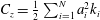$C_{z}={\textstyle \frac{1}{2}}\sum _{i=1}^{N}a_{i}^{2}k_{i}$ the equations coincide with the expansion derived by Nouguier et al. (Reference Nouguier, Chapron and Guérin2015) for the same quantity. By analogy with the first-order case, this latter version of the second-order expansion specified on the free surface ( $z_{0}=0$ ) will be referred to as the second-order CWM, or ‘CWM2’, in the following.

After some algebraic simplifications that occur for $z_{0}=0$ and using the linear dispersion relationship, the complete CWM2 expansion reads

(4.12) $$\begin{eqnarray}\displaystyle \left.\begin{array}{@{}c@{}}X(t)=x_{0}-\displaystyle \mathop{\sum }_{i=1}^{N}a_{i}\sin \unicode[STIX]{x1D713}_{i}^{0}+\mathop{\sum }_{i<j}a_{i}a_{j}B_{ij}^{x}(\sin \unicode[STIX]{x1D713}_{ij}^{0}-\sin \unicode[STIX]{x1D713}_{ij}^{0}|_{t=0})+{\mathcal{U}}_{s0}t\\[12.0pt] Z(t)=\frac{1}{2}\displaystyle \mathop{\sum }_{i=1}^{N}a_{i}^{2}k_{i}+\mathop{\sum }_{i=1}^{N}a_{i}\cos \unicode[STIX]{x1D713}_{i}^{0}+\mathop{\sum }_{i<j}a_{i}a_{j}B_{ij}^{z}\cos \unicode[STIX]{x1D713}_{ij}^{0},\end{array}\right\} & & \displaystyle\end{eqnarray}$$

where $\unicode[STIX]{x1D713}_{i}^{0}=k_{i}x_{0}-\unicode[STIX]{x1D714}_{i}t-\unicode[STIX]{x1D711}_{i}$ and $\unicode[STIX]{x1D713}_{ij}^{0}=\unicode[STIX]{x1D713}_{j}^{0}-\unicode[STIX]{x1D713}_{i}^{0}$ . Here ${\mathcal{U}}_{s0}$ is the total Stokes drift of the irregular wave field on the free surface, defined as

(4.13) $$\begin{eqnarray}\displaystyle {\mathcal{U}}_{s0}=\mathop{\sum }_{i=1}^{N}a_{i}^{2}k_{i}\unicode[STIX]{x1D714}_{i}, & & \displaystyle\end{eqnarray}$$

and,

(4.14) $$\begin{eqnarray}\displaystyle \left.\begin{array}{@{}c@{}}B_{ij}^{x}=k_{i}{\displaystyle \frac{\unicode[STIX]{x1D714}_{i}+\unicode[STIX]{x1D714}_{j}}{\unicode[STIX]{x1D714}_{i}-\unicode[STIX]{x1D714}_{j}}}\\[6.0pt] B_{ij}^{z}=k_{i}.\end{array}\right\} & & \displaystyle\end{eqnarray}$$

As compared to the CWM, the CWM2 includes wave interaction terms for both the horizontal and vertical position, represented by the double summations in (4.12). As was shown in Nouguier et al. (Reference Nouguier, Chapron and Guérin2015), only the wave interaction terms in $Z(t)$ are necessary to make this solution fully consistent with the second-order Eulerian expansion, while the wave interaction terms in $X(t)$ contribute only to third- and higher-order Eulerian expansion and, furthermore, are found to be numerically unstable. These double summations do not allow for an efficient numerical implementation of the CWM2 model as they require $O(N_{x}\times N)$ computations at every time step, where $N_{x}$ is the number of particle positions (corresponding to the grid of surface particles at rest) and $N$ the number of wave frequencies. On the contrary, the CWM model can be solved (Nouguier et al. Reference Nouguier, Guérin and Chapron2009) by a mere fast Fourier transform (FFT) which reduces the computational cost at every time step to $O(N\log N)$ . However, it will be shown later that the wave interaction terms have a negligible impact on the performance of the model for predicting the wave evolution in time. Hence, a numerically efficient version of the CWM2 model will be obtained by neglecting these interaction terms (that is keeping in the second-order terms only the Stokes drift and the mean vertical level correction).

4.3 The improved ‘choppy wave model’

As in the periodic wave case, the reference particle location $(\overline{x},\overline{z})$ will be optimized by requiring that it correspond to the mean particle location over a growing number of cycles. For irregular waves, the free surface is aperiodic but, for a sufficiently long time $t_{max}=nT_{p}\gg T_{p}$ (with $n$ a large integer number), it can be assumed that the harmonics in (4.9) and (4.11) nearly have a zero average. Hence, calculating the mean particle location to second order over the time interval $[0,t_{max}]$ and requiring that it be zero yields the (4.11) constants

(4.15) $$\begin{eqnarray}\displaystyle \left.\begin{array}{@{}c@{}}\displaystyle C_{x}=-\frac{1}{2}n\mathop{\sum }_{i=1}^{N}a_{i}^{2}k_{i}\unicode[STIX]{x1D714}_{i}\text{e}^{2k_{i}\overline{z}}T_{p}\\[6.0pt] C_{z}=0.\end{array}\right\} & & \displaystyle\end{eqnarray}$$

Note that the integration constant $C_{x}$ must be updated as the number of peak periods increases. As in the periodic wave case the free surface ( $z_{0}=0$ ) reference particle location is optimized after $n$ peak periods $(\overline{x}_{n},\overline{z}_{n})$ by requiring that the mean sea level (MSL) of the Lagrangian surface $\unicode[STIX]{x1D702}_{L}$ be zero. As we will see, this implies:

(4.16) $$\begin{eqnarray}\displaystyle \overline{z}_{n}=\overline{z}=\frac{1}{2}\mathop{\sum }_{i=1}^{N}a_{i}^{2}k_{i}, & & \displaystyle\end{eqnarray}$$

which is similar to (3.17) for regular waves.

Next the locus of surface particles (obtained with (4.16)) is derived, which implicitly defines an Eulerian surface $Z(t)=\unicode[STIX]{x1D702}_{L}(X(t))$ . Based on (4.9), the first-order displacement with respect to the reference position $(\overline{x},\overline{z})$ reads

(4.17) $$\begin{eqnarray}\displaystyle \left.\begin{array}{@{}c@{}}x_{1}(t)=\displaystyle -\mathop{\sum }_{i=1}^{N}a_{i}\sin \overline{\unicode[STIX]{x1D713}}_{i}=-D_{1}(\overline{x},t)\\[6.0pt] z_{1}(t)=\displaystyle \mathop{\sum }_{i=1}^{N}a_{i}\cos \overline{\unicode[STIX]{x1D713}}_{i}=\unicode[STIX]{x1D702}_{1}(\overline{x},t),\end{array}\right\} & & \displaystyle\end{eqnarray}$$

where $\unicode[STIX]{x1D702}_{1}$ is the linear surface elevation from (4.2) and $D_{1}$ is its Hilbert transform. At the second-order, equation (4.11) combined with (4.15) yields

(4.18) $$\begin{eqnarray}\displaystyle \left.\begin{array}{@{}c@{}}x_{2}(t)=\displaystyle \mathop{\sum }_{i<j}a_{i}a_{j}B_{ij}^{x}(\sin \overline{\unicode[STIX]{x1D713}}_{ij}-\sin \overline{\unicode[STIX]{x1D713}}_{ij}|_{t=0})+{\mathcal{U}}_{s0}\left(t-\frac{1}{2}nT_{p}\right)\\[6.0pt] z_{2}(t)=\displaystyle \mathop{\sum }_{i<j}a_{i}a_{j}B_{ij}^{z}\cos \overline{\unicode[STIX]{x1D713}}_{ij},\end{array}\right\} & & \displaystyle\end{eqnarray}$$

where the Stokes drift ${\mathcal{U}}_{s0}$ is defined in (4.13) and the kernels are given in (4.14). By comparing the modified second-order expansion (4.18) with the original CWM2, we see that the mean horizontal position $\overline{x}_{n}$ is related to the position at rest through $x_{n}=x_{0}+{\textstyle \frac{1}{2}}n{\mathcal{U}}_{s0}T_{p}$ . Therefore, for large $n$ , $\overline{x}$ can be replaced by $x_{0}+{\textstyle \frac{1}{2}}{\mathcal{U}}_{s0}t$ in (4.17) and (4.18), which amounts to replacing $\overline{\unicode[STIX]{x1D713}}_{i}$ by $\tilde{\unicode[STIX]{x1D713}}_{i}=k_{i}x_{0}-\tilde{\unicode[STIX]{x1D714}}_{i}t-\unicode[STIX]{x1D711}_{i}$ and $\overline{\unicode[STIX]{x1D713}}_{ij}$ by $\tilde{\unicode[STIX]{x1D713}}_{ij}=\tilde{\unicode[STIX]{x1D713}_{j}}-\tilde{\unicode[STIX]{x1D713}_{i}}$ in (4.17) and (4.18), with the modified angular frequency

(4.19) $$\begin{eqnarray}\displaystyle \tilde{\unicode[STIX]{x1D714}}_{j}=\unicode[STIX]{x1D714}_{j}-{\textstyle \frac{1}{2}}k_{j}{\mathcal{U}}_{s0}. & & \displaystyle\end{eqnarray}$$

The double summations in the expressions of $x_{2}$ and $z_{2}$ , in (4.17) and (4.18), which represent interaction terms between various harmonics, cannot efficiently be computed (i.e. by a FFT). However, even though their absolute value is of the same order of magnitude as the secular and constant terms in these equations, their fluctuating contributions to the free surface motion average out over a large time and, hence, can be neglected.

Consequently, equations (4.1), (4.17) and (4.18) yield the simplified expressions

(4.20) $$\begin{eqnarray}\displaystyle \left.\begin{array}{@{}c@{}}X(t)=x_{0}-\tilde{D}_{1}(x_{0},t)+{\mathcal{U}}_{s0}t\\[6.0pt] \displaystyle Z(t)=\tilde{\unicode[STIX]{x1D702}}_{1}(x_{0},t)+\frac{1}{2}\mathop{\sum }_{i=1}^{N}a_{i}^{2}k_{i},\end{array}\right\} & & \displaystyle\end{eqnarray}$$

where $\tilde{\unicode[STIX]{x1D702}}_{1}$ is a linear surface with modified angular frequency and $\tilde{D}_{1}$ is its Hilbert transform

(4.21) $$\begin{eqnarray}\displaystyle \left.\begin{array}{@{}c@{}}\displaystyle \tilde{\unicode[STIX]{x1D702}}_{1}(x,t)=\mathop{\sum }_{j=1}^{N}a_{j}\cos (k_{j}x-\tilde{\unicode[STIX]{x1D714}}_{j}t-\unicode[STIX]{x1D711}_{j}),\\[6.0pt] \displaystyle \tilde{D}_{1}(x,t)=-\mathop{\sum }_{j=1}^{N}a_{j}\sin (k_{j}x-\tilde{\unicode[STIX]{x1D714}}_{j}t-\unicode[STIX]{x1D711}_{j}).\end{array}\right\} & & \displaystyle\end{eqnarray}$$

An explicit but approximate formulation of the free surface elevation $Z=\unicode[STIX]{x1D702}_{L}(X,t)$ can be obtained at second order by inverting the relationship between $X$ and $x_{0}$ and performing a Taylor series expansion in the expression of $Z(t)$

(4.22) $$\begin{eqnarray}\displaystyle \left.\begin{array}{@{}c@{}}x_{0}\simeq X+\tilde{D}_{1}(X-{\mathcal{U}}_{s0}t,t)-{\mathcal{U}}_{s0}t\\ \displaystyle Z(t)\simeq \tilde{\unicode[STIX]{x1D702}}_{1}(X-U_{s}t,t)+\tilde{D}_{1}(X-{\mathcal{U}}_{s0}t,t){\displaystyle \frac{\unicode[STIX]{x2202}\tilde{\unicode[STIX]{x1D702}}_{1}}{\unicode[STIX]{x2202}x}}(X-{\mathcal{U}}_{s0}t,t)+\frac{1}{2}\mathop{\sum }_{i=1}^{N}a_{i}^{2}k_{i}.\end{array}\right\} & & \displaystyle\end{eqnarray}$$

Hence, based on (4.22) the nonlinear surface is defined as

(4.23) $$\begin{eqnarray}\displaystyle \unicode[STIX]{x1D702}_{L}(x,t)=\frac{1}{2}\mathop{\sum }_{i=1}^{N}a_{i}^{2}k_{i}+\tilde{\unicode[STIX]{x1D702}}_{1}(x-U_{s0}t,t)-\tilde{D}_{1}(x-{\mathcal{U}}_{s0}t,t){\displaystyle \frac{\unicode[STIX]{x2202}\tilde{\unicode[STIX]{x1D702}}_{1}}{\unicode[STIX]{x2202}x}}(X-{\mathcal{U}}_{s0}t,t)+\cdots & & \displaystyle\end{eqnarray}$$

or more explicitly as

(4.24) $$\begin{eqnarray}\displaystyle \unicode[STIX]{x1D702}_{L}(x,t) & = & \displaystyle \frac{1}{2}\mathop{\sum }_{i=1}^{N}a_{i}^{2}k_{i}+\mathop{\sum }_{j=1}^{N}a_{j}\cos (k_{j}(x-c_{j}t)-\unicode[STIX]{x1D711}_{j})\nonumber\\ \displaystyle & & \displaystyle -\,\mathop{\sum }_{i,j}a_{i}a_{j}k_{j}\sin (k_{i}(x-c_{i}t)-\unicode[STIX]{x1D711}_{i})\sin (k_{j}(x-c_{j}t)-\unicode[STIX]{x1D711}_{j})+\cdots \,,\end{eqnarray}$$

where $c_{j}$ is the linear phase velocity of each component, $c_{0j}$ , modified by the Stokes drift

(4.25) $$\begin{eqnarray}\displaystyle c_{j}=c_{0j}+{\textstyle \frac{1}{2}}{\mathcal{U}}_{s0}, & & \displaystyle\end{eqnarray}$$

with $c_{0j}=\unicode[STIX]{x1D714}_{j}/k_{j}$ . Note that the resulting free surface is well centred about the horizontal plane ( $\langle \unicode[STIX]{x1D702}_{L}(x,t)\rangle =0$ ), which justifies the choice in (4.16) of the reference vertical value.

The solution (4.19)–(4.21), hereafter referred to as ICWM, constitutes an improved formulation of the choppy wave model, which should preserve its high numerical efficiency. Even though second-order interaction terms have been discarded in this model, it retains second-order contributions that are dominant in the time evolution of a wave packet. These are (i) a modified angular frequency (resulting in a modified dispersion relationship); (ii) the Stokes drift; and (iii) the correction of the mean water level bias (see also Clamond (Reference Clamond2007) and his discussion of Gerstner’s theory in appendix A). Note that, given spectral amplitudes $a_{j}$ and initial phases $\unicode[STIX]{x1D711}_{j}$ , a Lagrangian surface $(X(t),Z(t))$ can be efficiently generated with ICWM, at every time step and over a spatial grid $x_{0}$ , with the computational cost of 2 FFTs.

5.1 Reference dataset and error definition

A synthetic reference nonlinear ocean surface is first generated using the open source code ‘HOS-ocean’ (Ducrozet et al. Reference Ducrozet, Bonnefoy, Le Touzé and Ferrant2016), which can accurately simulate the propagation of nonlinear waves over large spatio-temporal domains, up to a specified order in wave steepness, albeit at greater computational cost. Since its initial development by Dommermuth & Yue (Reference Dommermuth and Yue1987) and West et al. (Reference West, Brueckner, Janda, Milder and Milton1987), the HOS method has been extensively validated and used in various applications, such as the simulation of freak waves (Ducrozet et al. Reference Ducrozet, Bonnefoy, Le Touzé and Ferrant2007), the implementation of a numerical wave tank (Bonnefoy et al. Reference Bonnefoy, Ducrozet, Le Touzé and Ferrant2009) and ocean wave field reconstructions based on measurements (Blondel-Couprie et al. Reference Blondel-Couprie, Bonnefoy and Ferrant2013; Qi et al. Reference Qi, Wu, Liu, Kim and Yue2018a ). HOS-ocean solves the fully nonlinear potential flow problem as a function of time, in terms of $N$ complex amplitudes $A_{i}(t)$ , for many wave components $i$ , which are then used to reconstruct the ocean surface at an arbitrary point $\left(x,t\right)$ , as (in two dimensions)

(5.1) $$\begin{eqnarray}\displaystyle \unicode[STIX]{x1D702}_{HOS}\left(x,t\right)=\text{Re}\left(\mathop{\sum }_{j=1}^{N}A_{j}(t)\text{e}^{\text{i}k_{j}x}\right). & & \displaystyle\end{eqnarray}$$

In the following applications, we use a fifth-order HOS method with 32 grid points per peak wavelength $\unicode[STIX]{x1D706}_{p}$ , which was verified to provide converged results in terms of order of nonlinearity as well as discretization.

(i) We compare the time evolution of the relative root-mean-square (r.m.s.) difference between the Lagrangian surface $\unicode[STIX]{x1D702}_{LAG}$ (which can be generated either with CWM2 or ICWM) and the HOS surface elevation $\unicode[STIX]{x1D702}_{HOS}$ at the same points. Given that the Lagrangian surface is implicitly defined by the surface particle locations, it is much easier to perform this comparison on the Lagrangian grid (that is, the ensemble of points $(X(t),Z(t))$ ) rather than the Eulerian grid $(x,\unicode[STIX]{x1D702}_{LAG}(x))$ which requires an explicit formulation of the Lagrangian surface (which can only be attained in an approximate way).

The r.m.s. difference between a free surface representation and the HOS solution is thus defined as

(5.2) $$\begin{eqnarray}\displaystyle \unicode[STIX]{x1D716}_{LAG}\left(t\right)={\displaystyle \frac{1}{\text{rmsh}}}\left(\frac{1}{L}\int _{0}^{L}\{Z\left(t\right)-\unicode[STIX]{x1D702}_{HOS}(X(t),t)\}^{2}\,\text{d}X(t)\right)^{1/2}, & & \displaystyle\end{eqnarray}$$

where $L$ is the computational domain length and the normalization constant ‘ $\text{rmsh}$ ’ is defined as

(5.3) $$\begin{eqnarray}\displaystyle \text{rmsh}=\left({\displaystyle \frac{1}{L}}\int _{0}^{L}\unicode[STIX]{x1D702}_{HOS}^{2}(x,0)\,\text{d}x\right)^{1/2}=\left(\frac{1}{2}\mathop{\sum }_{i=1}^{N}\left|A_{i}(0)\right|^{2}\right)^{1/2} & & \displaystyle\end{eqnarray}$$

and represents the r.m.s. elevation of the initial surface, which we also express as a function of spectral amplitudes $A_{i}(0)$ .

(ii) Given the initial wave spectrum of an irregular surface, the corresponding free surface elevation in the HOS model follows a modified energy density spectrum, due to nonlinear wave–wave interactions and the redistribution of energy that occurs during wave propagation. Hence free surface statistics are not stationary and thus not fully controlled during the nonlinear time evolution. By contrast, CWM surfaces, which are based on a spatial transformation of a linear surface, with a prescribed underlying spectrum, in principle have stationary statistics (that is, their wave spectrum should not evolve in time, even though it can be modified by the bound waves). Hence, a meaningful comparison between time-evolving surfaces in different models can only be performed within smaller time intervals, within which statistics (essentially the energy density spectrum) can be assumed to be stationary. A measure of differences between the initial spectrum and the evolving spectrum of HOS surfaces is given by the r.m.s. difference

(5.4) $$\begin{eqnarray}\displaystyle \displaystyle \unicode[STIX]{x1D716}_{spec}\left(t\right)={\displaystyle \frac{\left(\displaystyle \mathop{\sum }_{i=1}^{N}(|A_{i}(t)|-|A_{i}(0)|)^{2}\right)^{1/2}}{\left(\displaystyle \mathop{\sum }_{i=1}^{N}|A_{i}(0)|^{2}\right)^{1/2}}}. & & \displaystyle\end{eqnarray}$$

This measure thus provides a lower threshold to the error of Lagrangian methods $\unicode[STIX]{x1D716}_{LAG}\left(t\right)$ (defined by (5.2)), which therefore provides a relevant indicator of the method performance only if, $\unicode[STIX]{x1D716}_{spec}\left(t\right)\ll \unicode[STIX]{x1D716}_{LAG}\left(t\right)$ . In practice, for the typical wave spectra under consideration, we found that this is the case for an evolution time smaller than approximately 20–40 $T_{p}$ , depending on wave steepness.

(iii) Given an energy density spectrum, phases must be provided for each wave component to generate an initial free surface, which is then propagated in the various models. A rigorous comparison of time-evolving surfaces should thus be based on identical sets of (random or deterministic) initial phases. However, such phases can only be prescribed for linear surfaces but not for Lagrangian or HOS surfaces, which undergo a nonlinear transformation. To mitigate possible discrepancies arising from the choice of initial phases, the HOS model is initialized with an explicit nonlinear solution, which is close to the Lagrangian solution (Perignon et al. Reference Perignon, Bonnefoy, Ferrant and Ducrozet2010; Perignon Reference Perignon2011), namely the second-order Eulerian Stokes solution for irregular wave fields as detailed in Longuet-Higgins (Reference Longuet-Higgins1963). The same underlying linear surface can be used to generate Lagrangian surfaces in the second-order expansions (CWM2, ICWM), through a geometrical transformation based on the Hilbert transform.

5.2 Periodic waves

Let us first consider a strongly nonlinear periodic wave of steepness $H/\unicode[STIX]{x1D706}\simeq 0.08$ and period $T$ , where $H=2a$ is the wave height and $\unicode[STIX]{x1D706}$ the wavelength; for linear deep-water waves, $T=\sqrt{2\unicode[STIX]{x03C0}\unicode[STIX]{x1D706}/g}$ . This steepness is over half the deep water limiting steepness and corresponds to $ka\simeq 0.25$ , which is in the domain of applicability of the Lagrangian approach (Pierson Reference Pierson1961). For periodic waves, free surfaces represented in the various models can be easily synchronized at initial time, using the same phase as that of the fundamental component of the HOS solution. A domain of length equal to one wavelength is used to evaluate the error.

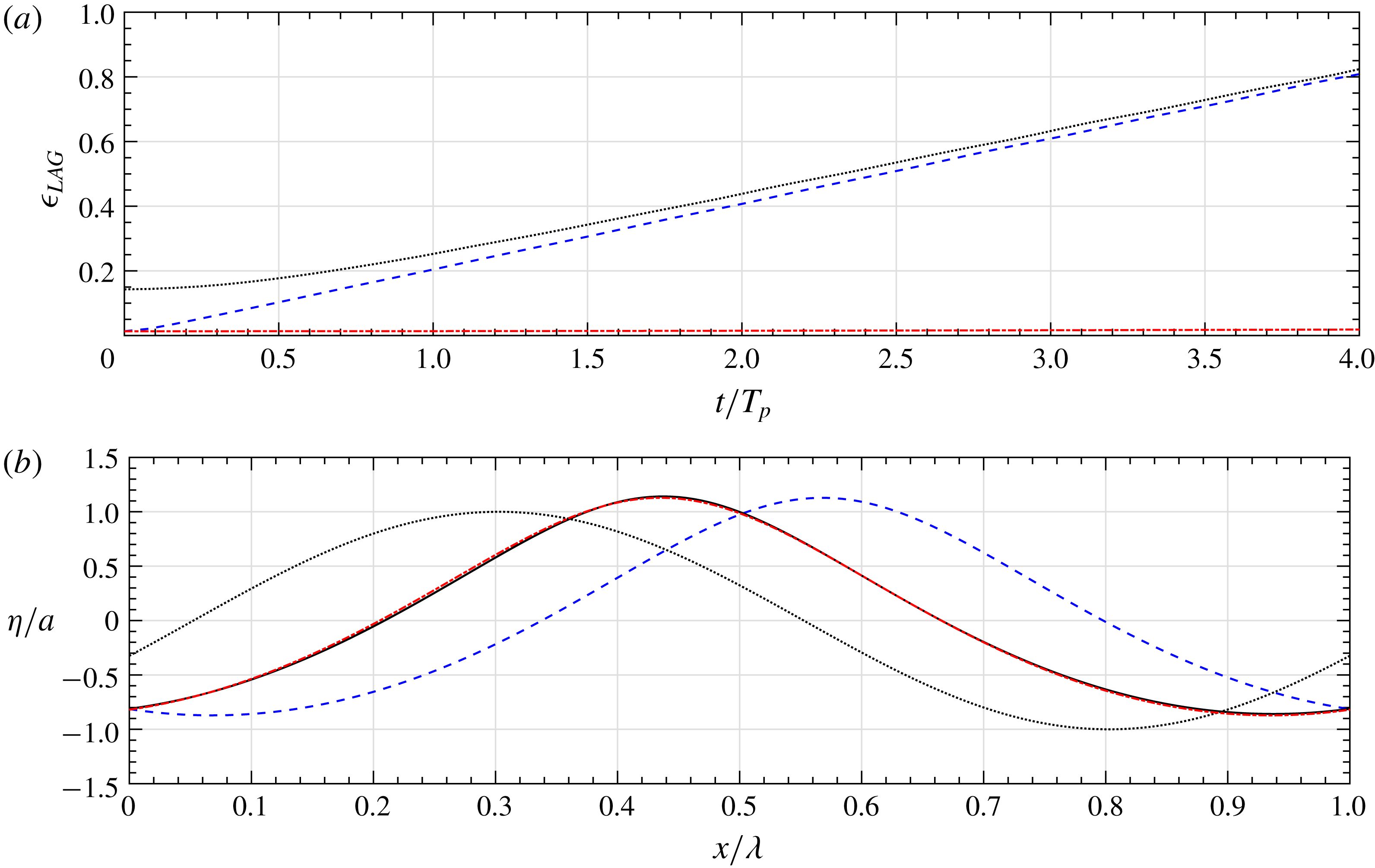
Figure 2(a) shows that, at $t=0$ , the CWM2 and ICWM surface elevations are identical since time dependent terms vanish. Both solutions also match quite well the HOS solution (very small errors can be seen in the figure), and much better than the linear solution, whose error is $\unicode[STIX]{x1D716}_{LAG}(0)\simeq 0.15$ , due to an inaccurate wave shape. In figure 2(a), the errors for the CWM2 and linear model follow a parallel growth: while the linear wave does not experience nonlinear phase velocity corrections, CWM2 is penalized by an overestimated nonlinear correction (close to twice the correct value, as discussed in § 2). By contrast, for ICWM, the improved estimate of the nonlinear phase shift allows for errors to remain very small throughout the four-period propagation time considered here. At this stage, figure 2(b) shows a very marked phase shift of the linear and CWM2 model results with respect to the HOS reference solution, whereas no measurable shift is seen for the ICWM solution.

5.3 Irregular waves

Figure 2.

Comparison of results computed for a periodic wave of steepness $H/\unicode[STIX]{x1D706}\simeq 8\,\%$ , with the HOS (——), linear ( $\cdots \cdots$ ), CWM2 (- - -) and ICWM (– - – - –) models: (a) error as a function of time with respect to the HOS solution; (b) normalized free surface elevations after approximately four periods of propagation.

Figure 3.

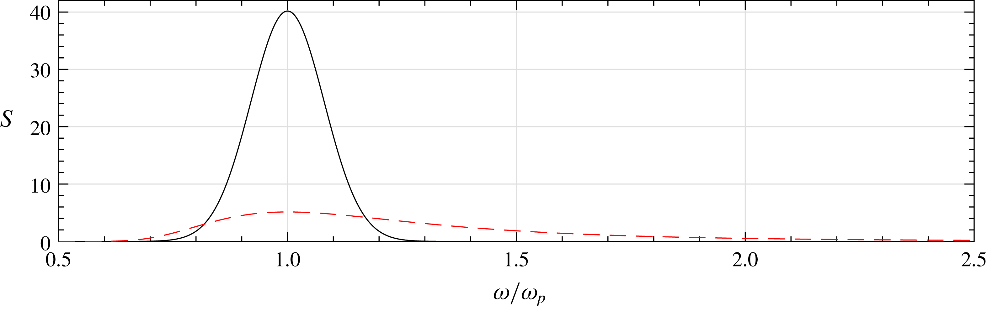
Energy density spectrum as a function of the dimensionless angular frequency $\unicode[STIX]{x1D714}/\unicode[STIX]{x1D714}_{p}$ , for a narrow (Gauss, solid line) or broad-banded (JS, red dashed line) spectrum. The characteristic steepness is $H_{s}/\unicode[STIX]{x1D706}_{p}\simeq 6\,\%$ and 4 % for each case, respectively.

The performance of the improved Lagrangian formulation is now assessed for irregular waves generated on the basis of a specified energy density spectrum $S(\unicode[STIX]{x1D714})$ (see figure 3). Similar to the periodic wave case, we investigate the time evolution of the error of the CWM2, ICWM and linear solutions, with respect to the HOS reference solution. Given a sea state of parameters $(H_{s},T_{p})$ , the influence of energy spreading around the peak spectral frequency on the performance of the various wave models is investigated by considering two different spectra: (i) a narrow-banded Gaussian spectrum

(5.5) $$\begin{eqnarray}\displaystyle S(\unicode[STIX]{x1D714})=\unicode[STIX]{x1D6FC}{\displaystyle \frac{1}{\sqrt{2\unicode[STIX]{x03C0}\unicode[STIX]{x1D70E}^{2}}}}\text{e}^{-((\unicode[STIX]{x1D714}-\unicode[STIX]{x1D714}_{p})^{2}/2\unicode[STIX]{x1D70E}^{2})}, & & \displaystyle\end{eqnarray}$$

of standard deviation $\unicode[STIX]{x1D70E}/\unicode[STIX]{x1D714}_{p}=0.08$ , where $\unicode[STIX]{x1D714}_{p}=2\unicode[STIX]{x03C0}/T_{p}$ denotes the peak angular frequency, and (ii) a JONSWAP (JS) spectrum with peakedness parameter $\unicode[STIX]{x1D6FE}=1$

(5.6) $$\begin{eqnarray}\displaystyle S(\unicode[STIX]{x1D714})=\unicode[STIX]{x1D6FC}{\displaystyle \frac{g^{2}}{\unicode[STIX]{x1D714}^{5}}}\text{e}^{-(5/4)(\unicode[STIX]{x1D714}_{p}/\unicode[STIX]{x1D714})^{4}} & & \displaystyle\end{eqnarray}$$

(i.e. similar to the Pierson–Moskowitz (PM) spectrum of a fully developed sea, but with fetch-dependent peak frequency). In both cases, parameter $\unicode[STIX]{x1D6FC}$ is found based on a specified $H_{s}$ value, from the standard definition

(5.7) $$\begin{eqnarray}\displaystyle \int _{0}^{\infty }S(\unicode[STIX]{x1D714})\,\text{d}\unicode[STIX]{x1D714}={\displaystyle \frac{H_{s}^{2}}{16}}. & & \displaystyle\end{eqnarray}$$

In the applications, we use $T_{p}=10$ s with $H_{s}=9$ m for the Gaussian spectrum and $H_{s}=6$ m for the JS spectrum. This yields characteristic deep-water steepnesses $H_{s}/\unicode[STIX]{x1D706}_{p}\simeq 6\,\%$ and $4\,\%$ , respectively, with $\unicode[STIX]{x1D706}_{p}=2\unicode[STIX]{x03C0}/k_{p}$ denoting the peak spectral wavelength (note that the corresponding PM spectrum would have $T_{p}=12.3$ s, i.e. the JS spectrum used here represents a fetch limited sea). The corresponding spectra are shown in figure 3.

For irregular waves, a larger number of dominant waves than in the periodic case must be modelled in the computational domain, in order to achieve convergence of the integral error of (5.2); here we use a spatial domain spanning eight peak wavelengths, i.e. $L=8\unicode[STIX]{x1D706}_{p}$ . At $t=0$ , the linear and CWM free surfaces are constructed from the linear spectral information using the same set of random phases. For the HOS model, however, unlike periodic waves, linear information cannot be retrieved (except at initialization time $t=0$ ) due to the implicit nonlinear components. Moreover, using linear information to initialize the HOS nonlinear propagation would lead to unstable calculations of higher-order terms (Dommermuth Reference Dommermuth2000). Hence, to allow for a deterministic comparison between models, the HOS was initialized solver with a nonlinear irregular wave field, here, a second-order Stokes wave solution, following the method detailed in Perignon et al. (Reference Perignon, Bonnefoy, Ferrant and Ducrozet2010) and Perignon (Reference Perignon2011).

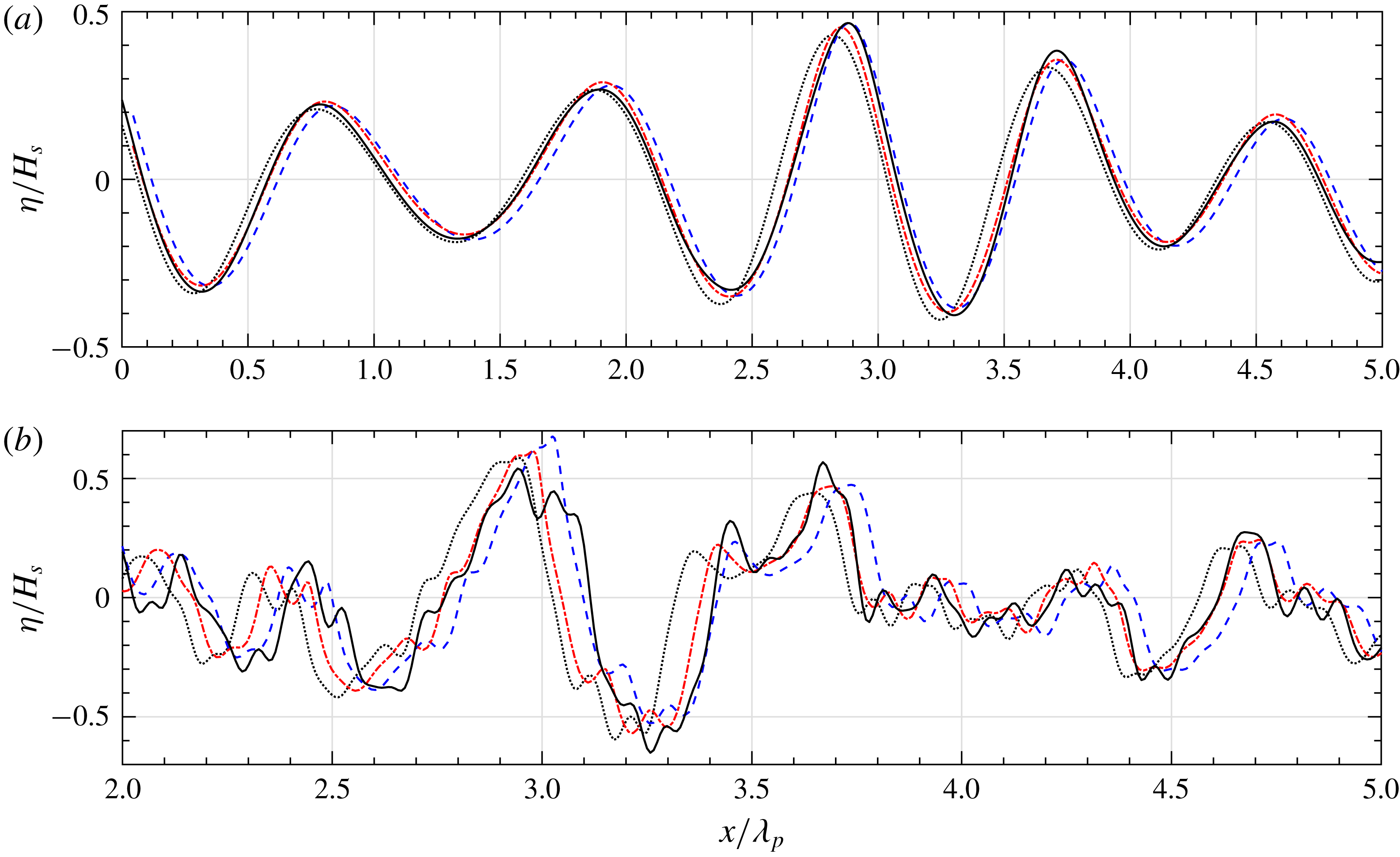
Figure 4 shows the comparison of normalized surface elevations computed in the different models at $t=4T_{p}$ , for the two types of spectra. For the wave train extracted from a Gaussian spectrum, figure 4(a) shows that the ICWM model prediction remains very accurate after $4T_{p}$ . With the other models, for which wave celerity is inaccurate, waves are either delayed (linear solution) or too fast (CWM2), with respect to the HOS reference solution. Similar observations can be made in figure 4(b), although in a less obvious way, for waves extracted from a JS spectrum: after $4T_{p}$ of propagation, the overall locations of dominant waves modelled with the ICWM model are consistent with the HOS solution (although not their smaller fluctuations), whereas the linear and CWM2 solutions are already desynchronized with it.

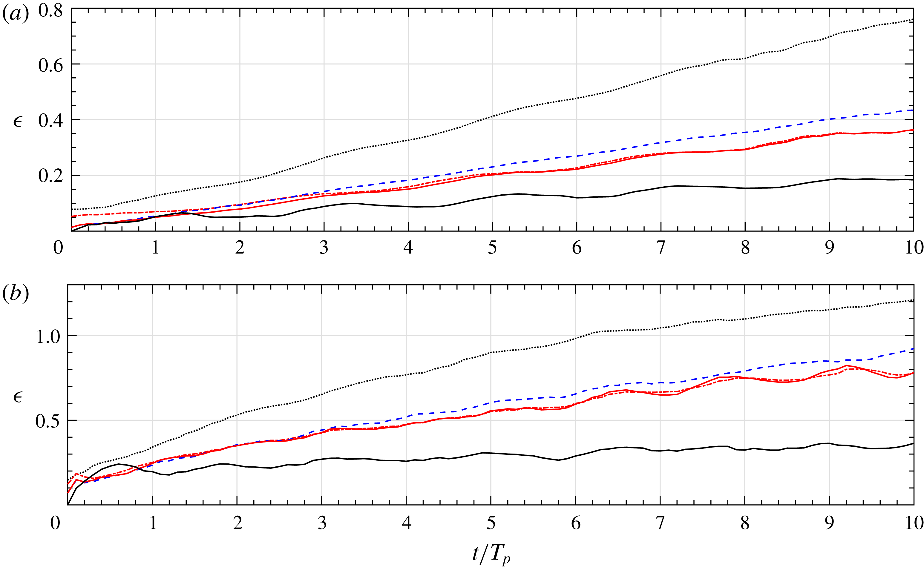
More specifically, figure 5 shows the time evolution of relative errors computed with (5.2) over the first 10 peak periods of propagation, for the two cases of figure 4. In the Gaussian spectrum case, the ICWM model yields errors reduced by a factor of ${\sim}2$ with respect to the linear solution as well as a significant improvement with respect to results of the CWM2 model. The overall error is larger in the JS spectrum case, but the same qualitative observations hold true. To quantify the effect of second-order interaction terms, which have been discarded in the ICWM model to obtain a numerically efficient solution, the CWM2 model results with a corrected dispersion relationship (4.19) have also been computed (referred to as ‘ICWM with interaction terms’ in figure 5). As seen in the figures, these terms only yield significant effects within the first peak period of propagation (particularly in the Gaussian case) and become rapidly negligible with respect to the correction due to the dispersion relationship (ICWM). The black lines in figure 5 show the relative variation of the wave energy spectrum of the HOS reference surface, which is verified to remain small with respect to the relative error between methods. This confirms that the improved accuracy of ICWM for wave prediction is essentially due to a corrected wave celerity rather than an accurate description of bound waves.

We also checked the relative importance of the horizontal displacement term $\tilde{D}_{1}$ in (4.20) with respect to the wave celerity correction; to do so, we simulated the evolving surface according to LWT (not shown here), but using the corrected nonlinear dispersion relationship (CDR) (i.e. (4.23) with $\tilde{D}_{1}=0$ ), a model henceforth referred to as LWT-CDR. At initial time, when it represents a purely linear surface, LWT-CDR yields a significantly larger relative error than ICWM (as can be seen in figures 2 and 5 at $t=0$ ). However, after a few peak periods of propagation, we find that the LWT-CDR and ICWM solutions yield comparable errors, showing once again that, as far as predicting surface elevations, the dominant source of error is inaccuracies in wave celerity.

Note that numerical results are only shown in figure 5 for a single steepness for each spectrum ( $6\,\%$ or $4\,\%$ ), which in fact represents the largest value achievable with the HOS model. At larger steepnesses, this model breaks down after a few periods due to the occurrence of wave breaking in the simulated sea state, which is not explicitly treated in the version of HOS-ocean used in this study (Ducrozet, Bonnefoy & Perignon Reference Ducrozet, Bonnefoy and Perignon2017). We performed a more systematic numerical investigation of the effect of wave steepness, which showed as could be expected that gradually increasing it both increases discrepancies between the linear and nonlinear model results and yields larger errors as time increases. For small steepness, the effect of interaction terms is negligible while the divergence of the linear model is still significant in the long term.

Figure 4.

Normalized surface elevations computed with: HOS (——), linear ( $\cdots \cdots$ ), CWM2 (- - -) and ICWM (– - – - –) models, after $t=4T_{p}$ of propagation, for irregular wave trains with $T_{p}=10$ s extracted from a (a) Gaussian spectrum with standard deviation $\unicode[STIX]{x1D70E}/\unicode[STIX]{x1D714}_{p}=0.08$ , $H_{s}=9~\text{m}$ and characteristic steepness $H_{s}/\unicode[STIX]{x1D706}_{p}\simeq 6\,\%$ ; and (b) a JS spectrum with peakedness parameter $\unicode[STIX]{x1D6FE}=1$ (similar to a PM spectrum), $H_{s}=6~\text{m}$ and $H_{s}/\unicode[STIX]{x1D706}_{p}\simeq 4\,\%$ . See figure 3 for spectral shapes.

Figure 5.

Time evolution of relative errors (5.2) for the two cases of figure 4 (a,b), for the linear ( $\cdots \cdots$ ), CWM2 (- - -), ICWM (– - – - –) and ICWM with interaction terms (——) model results. The black solid line shows the relative change (5.4) of the prescribed spectrum during the HOS time evolution.

An important final remark is that criterion (5.2), used to quantify the error with respect to a rigorous model, is based on the r.m.s. of the surface elevations, which is mostly impacted by long waves. However, when it comes to predicting or interpreting properties of radar or LIDAR beams scattered by the sea surface, the accurate description of the free surface roughness at small scale becomes crucial. In this context, the improvement of the ICWM over LWT or LWT-CDR models is not only related to its kinematical correction (which was found to be dominant in the present numerical analyses), but also to its geometrical correction of wave shape, which more significantly affects free surface slopes. Additional work is in progress to evaluate the performance of the ICWM from this ‘small scale roughness’ point of view.