





1. Introduction
Dense granular suspensions, i.e. suspensions of non-Brownian particles in liquids, can be found in many natural settings, such as debris flows (Kostynick et al. Reference Kostynick, Matinpour, Pradeep, Haber, Sauret, Meiburg, Dunne, Arratia and Jerolmack2022), and play vital roles in many aspects of human life, including engineering (e.g. cement (Richards et al. Reference Richards, Li, O’Neill, Laidlaw and Royer2024)), food (e.g. juices (Leverrier et al. Reference Leverrier, Augusto and Menut2025) and chocolate (Blanco et al. Reference Blanco, Hodgson, Hermes, Besseling, Hunter, Chaikin, Cates, Damme and Poon2019)) and medicine (e.g. drugs delivered in liquid suspension form (Visser et al. Reference Visser, Seldam, van der Linden, Hinrichs, Veenendaal, Dijkers and Woerdenbag2018)).
The rheology of non-Brownian suspensions has been studied from a fluid dynamic perspective since the beginning of the 20th century, when Einstein (Reference Einstein1911) derived the first-order correction to the viscosity of a dilute suspension of rigid spheres in Stokes flow
 \begin{equation} \eta =\eta _f\left (1+\frac {5}{2}\phi \right )+O(\phi ^2) \end{equation}
(where
 $\phi$
is the solid volume fraction and
 $\eta _f$
is the dynamic viscosity of the suspending fluid), with a correction for non-negligible particle inertia found by Lin et al. (Reference Lin, Peery and Schowalter1970), and a correction to
 $O(\phi ^2)$
found by Batchelor & Green (Reference Batchelor and Green1972).
However, a single-phase model with a
 $\phi$
-dependent viscosity has been shown to be insufficient to describe the flow of non-Brownian suspensions for larger values of
 $\phi$
. The coefficient of the
 $\phi ^2$
term is known to depend on flow type (Mewis & Wagner Reference Mewis and Wagner2011), and as the suspensions become more concentrated, the particles contribute increasingly significant normal forces to the suspension (Batchelor Reference Batchelor1970; Deboeuf et al. Reference Deboeuf, Gauthier, Martin, Yurkovetsky and Morris2009), often described in the form of an effective solid pressure
 $p_s$
(i.e. an isotropic stress in excess of the hydrostatic pressure). In fixed-volume simple shear, the effective pressure is seen to grow proportionally with the imposed shear rate
 $\dot \gamma$
, defining an effective normal viscosity,
 $\eta _n(\phi )\equiv p_s/(\eta _f\dot \gamma )$
. Normal stress differences are also observed at sufficiently large values of
 $\phi$
(Dai et al. Reference Dai, Bertevas, Qi and Tanner2013).
In the dense regime (which we define by
 $\phi \gtrsim 0.1$
), similarities emerge between non-Brownian suspensions and granular flows, where the interstitial fluid is of negligible viscosity. In granular flows, the behaviour changes substantially as the volume fraction varies, from a granular gas at low volume fraction (Brilliantov & Pöschel Reference Brilliantov and Pöschel2004), through an inertial regime at intermediate volume fractions (Berzi Reference Berzi2024), to a quasi-static regime close to a maximum volume fraction
 $\phi _m$
. In the inertial regime, the flow has been shown to depend only on the inertial number
 \begin{equation} I\equiv \frac {\dot \gamma d}{\sqrt {p_s/\rho _s}} \end{equation}
in steady shear flows (Gdr MiDi Reference MiDi2004; da Cruz et al. Reference da Cruz, Emam, Prochnow, Roux and Chevoir2005), where
 $d$
is the grain diameter and
 $\rho _s$
is the solid density. This number can be seen as representing a ratio of time scales, with
 $d/\sqrt {p_s/\rho _s}$
the time scale associated with acceleration of the grains by normal forces, and
 $1/\dot \gamma$
the time scale for deformation by shear. The inertial number can be controlled experimentally in simple shear by altering the set-up to impose normal stress
 $p_s$
and allow the flow to dilate, rather than imposing volume fraction
 $\phi$
, as in a fixed-volume shear cell. Simple constitutive laws have been found in terms of
 $I$
for the friction coefficient
 $\mu =\tau /p_s$
(where
 $\tau$
is the shear stress), and the solid volume fraction
 $\phi$
(Jop et al. Reference Jop, Forterre and Pouliquen2006; Pouliquen et al. Reference Pouliquen, Cassar, Jop, Forterre and Nicolas2006). Those studies find that the function
 $\mu (I)$
takes a finite value
 $\mu _1$
at
 $I=0$
, indicating a pressure-dependent yield stress
 $\mu _1p_s$
, and is increasing for
 $I\gt 0$
, while the function
 $\phi (I)$
attains its maximum value
 $\phi _m$
at
 $I=0$
, representing jamming, and is decreasing for
 $I\gt 0$
, indicating dilation. However, functions
 $\mu (I)$
have been observed with non-monotonicity near jamming in simulations (Ness & Fielding Reference Ness and Fielding2025), which can lead to shear banding, as seen experimentally (Wolf et al. Reference Wolf, König and Triantafyllidis2003).
It has been shown that dense granular suspensions can be described similarly (Boyer et al. Reference Boyer, Guazzelli and Pouliquen2011), with some modifications to the theory. The inertial number
 $I$
is replaced by the viscous number
 \begin{equation} J\equiv \frac {\eta _f\dot \gamma }{p_s}, \end{equation}
indicating the dominance of viscous over inertial effects. The relevant time scale for pressure-related deformation is now
 $\eta _f/p_s$
, with the condition
 $J\gg I^2$
corresponding to a small Stokes number
 $\textit {St}=\rho _sd^2\dot \gamma /\eta _f$
. The form of (1.3) reflects the observation that in fixed-volume simple shear, the solid pressure
 $p_s$
increases proportionally with the imposed shear rate
 $\dot \gamma$
(Deboeuf et al. Reference Deboeuf, Gauthier, Martin, Yurkovetsky and Morris2009). The functions
 $\mu (J)$
and
 $\phi (J)$
can then be found empirically. They share several features with the granular flow functions
 $\mu (I)$
and
 $\phi (I)$
, with
 $\mu (J)$
also typically an increasing function with a non-zero value at
 $J=0$
, and
 $\phi (J)$
a decreasing function attaining its maximum
 $\phi _m$
at
 $J=0$
. However, non-monotonic functions
 $\mu (J)$
have also been observed in simulations, as in the dry granular case, by Ness & Fielding (Reference Ness and Fielding2025).
The
 $\mu (J)$
model was derived from simple steady shear experiments, with uniform normal and shear stress fields. The accuracy of its predictions in flows with inhomogeneous stress fields is an important question; in particular, few flows have been investigated analytically, a process that can shed light on the potential deficiencies of the model in complex flow geometries and inform future modifications.
Due to the dependence of the
 $\mu (J)$
model on normal stresses
 $p_s$
, it is desirable to investigate its predictions in flows with inhomogeneous normal stresses, as well as shear stress inhomogeneities. The former can be done by introducing gravity, as in the study of viscous resuspension, the ability of viscous shear to dilate and fluidise a settled bed of neutrally buoyant grains (Leighton & Acrivos Reference Leighton and Acrivos1986; d’Ambrosio et al. Reference d’Ambrosio, Blanc and Lemaire2021), while the latter can be found in pressure-driven flows (Nott & Brady Reference Nott and Brady1994; Orsi et al. Reference Orsi, Lobry, Lemaire and Peters2024). The two can then be combined in a pressure-driven duct flow in the presence of gravity, and several flow configurations have been found experimentally in this geometry. For example, Aussillous et al. (Reference Aussillous, Chauchat, Pailha, Médale and Guazzelli2013) and Meeker et al. (Reference Meeker, Gadon, Abdelouahab, Ovarlez and Bodiguel2020) have studied the transport of grains along the bottom of a fluid-filled horizontal rectangular duct, an example of a bedload flow. A distinct qualitative regime is found if the duct is nearly filled with submerged grains, and this regime has been investigated experimentally by Morgan et al. (Reference Morgan, James, Barron and Sandnes2020) and Morgan & Taylor-West (Reference Morgan and Taylor-West2024), through a range of density differences, flow rates and duct aspect ratios. This is the regime that will be the focus of our experiments. These latter investigations included measurements of grain velocity profiles and suspension flux through the ducts, with the experiments of Morgan et al. (Reference Morgan, James, Barron and Sandnes2020) additionally measuring grain volume fraction profiles and grain flux. However, neither investigation had access to the driving fluid pressure gradient, an important system parameter, which we obtain experimentally in this study.
In this paper, we model the steady pressure-driven flow of a dense granular suspension through a tall, thin rectangular duct, in the presence of gravity. In §§ 2 and 3, we set out the governing equations according to the
 $\mu (J)$
model. In §§ 4 and 5, we model suspension flow in ducts with smooth and rough side walls, respectively. In § 6, we carry out experiments to test the model predictions.
2. Mathematical model
2.1. Rheology
We use the
 $\mu (J)$
model of Boyer et al. (Reference Boyer, Guazzelli and Pouliquen2011), which gives equations for the friction coefficient
 $\mu \equiv \tau /p_s$
(where
 $\tau$
is the shear stress and
 $p_s$
is the solid pressure) and the solid volume fraction
 $\phi$
in terms of the viscous number
 $J\equiv \eta _f\dot \gamma /p_s$
, where
 $\eta _f$
is the fluid viscosity and
 $\dot \gamma$
is the grain shear rate. These functions take the empirically determined forms
 \begin{equation} \mu (J)=\underbrace {\mu _1+\frac {\mu _2-\mu _1}{1+J_0/J}}_{\mu _c(J)}+\underbrace {\vphantom {\frac {\mu _2-\mu _1}{1+J_0/J}}\frac {5}{2}\phi _mJ^{1/2}+J}_{\mu _h(J)},\quad \phi (J)=\frac {\phi _m}{1+J^{1/2}}. \end{equation}
The functions
 $\mu$
,
 $\mu _c$
,
 $\mu _h$
and
 $\phi$
are plotted in figure 1. The constants
 $\mu _1,\mu _2,J_0$
and
 $\phi _m$
are found empirically, and are given by the values in table 1. These values will be used throughout the theoretical part of this paper, in §§ 2–5. In particular,
 $\phi _m$
represents the maximum solid fraction, attained when
 $J=0$
, and
 $\mu _1$
represents the minimum friction
 $\mu$
required for deformation, implying a yield stress
 $\mu _1p_s$
. Below this yield stress, i.e. for
 $\tau /p_s\leqslant \mu _1$
, the equations
 $\dot \gamma =0$
and
 $\phi =\phi _m$
are instead satisfied.
Values of the constants in (2.1), as found experimentally by Boyer et al. (Reference Boyer, Guazzelli and Pouliquen2011). These values are used throughout the theoretical part of this paper, in §§ 2–5.

Table 1. Long description
The parameters are defined by phi sub m equals 0.585, mu sub 1 equals 0.32, mu sub 2 equals 0.7, and J sub 0 equals 0.005.


The form of (2.1a
) was chosen to match various existing theories. The final term
 $J$
represents the stress from fluid viscosity alone, while
 $(5/2)\phi _mJ^{1/2}$
corresponds at small
 $\phi$
to the
 $O(\phi )$
term in (1.1), together representing leading-order hydrodynamic effects. In contrast, the first two terms in (2.1a
) have the same form as the dry granular flow law
 $\mu (I)$
as found by Jop et al. (Reference Jop, Forterre and Pouliquen2006), and are hence interpreted as representing contacts between grains. These hydrodynamic and contact contributions to
 $\mu$
are plotted in figure 1(
 $a$
).
Equations (2.1a,b
) are written in terms of scalar
 $J$
and
 $\mu$
, as derived in simple shear experiments. To apply the model to more general geometries, it is necessary to write these scalars in terms of higher-dimensional tensor quantities. Defining the solid velocity
 $\boldsymbol{u}_s$
, we can write the solid shear rate tensor and its magnitude
 \begin{equation} \boldsymbol{\dot \gamma }=\boldsymbol{\nabla }\boldsymbol u_s+\boldsymbol{\nabla }\boldsymbol u_s^T,\quad \dot \gamma =\sqrt {\frac {1}{2}\boldsymbol{\dot \gamma }{:}\boldsymbol{\dot \gamma }}, \end{equation}
and we define the shear stress tensor
 $\boldsymbol \tau$
and its magnitude
 $\tau =\sqrt {({1}/{2})\boldsymbol \tau {:}\boldsymbol \tau }$
similarly. We also assume that the shear stress and shear rate tensors are aligned, so that
 $\boldsymbol \tau /p_s=\mu (J)\boldsymbol{\dot \gamma }/\dot \gamma$
whenever
 $\dot \gamma \gt 0$
. Since the suspension can dilate, the tensor
 $\boldsymbol{\dot \gamma }$
is not necessarily traceless, and hence this equation implies that
 $\boldsymbol \tau$
is not necessarily deviatoric. To remedy this, it is possible to align
 $\boldsymbol \tau$
with the traceless part of
 $\boldsymbol{\dot \gamma }$
instead. Alternatively,
 $\boldsymbol{\dot \gamma }$
could be calculated from the incompressible mixture flux
 $\boldsymbol U=\phi \boldsymbol u_s+(1-\phi )\boldsymbol u_f$
, where
 $\boldsymbol u_f$
is the fluid velocity, rather than from the solid velocity alone. However, in this paper, we will only consider shear flows, and hence
 $\boldsymbol{\dot \gamma }$
will be traceless throughout.
Within this framework, it is convenient to rewrite (2.1a,b
) in terms of tensor quantities, inverting
 $\phi (J)$
to replace
 $J$
with the more physically intuitive variable
 $\phi$
 \begin{equation} \begin{matrix} \boldsymbol \tau =\eta _f\eta _s(\phi )\boldsymbol{\dot \gamma },\quad p_s=\eta _f\eta _n(\phi )\dot \gamma &\text{if }\phi \lt \phi _m,\\ \tau \lt \mu _1p_s,\quad \dot \gamma =0&\text{if }\phi =\phi _m ,\end{matrix} \end{equation}
where the shear and normal viscosities are respectively defined
 \begin{equation} \eta _s(\phi )=1+\frac {5}{2}\phi _m\left (\frac {\phi _m}{\phi }-1\right )^{-1}+\left [\mu _1+\frac {\mu _2-\mu _1}{1+J_0/\left(\frac {\phi _m}{\phi }-1\right)^2}\right ]\left (\frac {\phi _m}{\phi }-1\right )^{-2}, \end{equation}
 \begin{equation} \quad \eta _n(\phi )=\left (\frac {\phi _m}{\phi }-1\right )^{-2}. \end{equation}
In this representation, it is clearer to see that the expression for
 $\eta _s(\phi )$
matches the asymptotic expansion for small
 $\phi$
, given in (1.1), up to
 $O(\phi )$
. The normal viscosity
 $\eta _n(\phi )$
also vanishes at
 $O(\phi )$
, fully recovering the dilute limit.
This tensorial formulation of the
 $\mu (J)$
model has been shown by Barker et al. (Reference Barker, Gray, Schaeffer and Shearer2023) to be ill-posed in transient flows, with high wavenumber perturbations in the solid fraction growing rapidly when
 $J$
is small. However, those authors also provided a regularised model, which converges in the steady limit to the
 $\mu (J)$
model described here. In this paper, we will only consider solutions to the steady
 $\mu (J)$
model, avoiding any issues of ill-posedness.
2.2. Kinematics and dynamics
We complete the two-phase description of the solid–fluid mixture by defining the fluid velocity
 $\boldsymbol{u}_f$
, and writing equations for conservation of mass and momentum. We neglect the effects of inertia throughout. The mass-conservation equations for the solid and fluid components, respectively, can be written
 \begin{equation} \frac {\partial \phi }{\partial t}+\boldsymbol{\nabla }\boldsymbol{\cdot }(\phi \boldsymbol{u}_s)=0,\quad \frac {\partial }{\partial t}(1-\phi )+\boldsymbol{\nabla }\boldsymbol{\cdot }((1-\phi )\boldsymbol{u}_f)=0, \end{equation}
and momentum conservation for the mixture can be written
 \begin{equation} -\boldsymbol{\nabla } p_s-\boldsymbol{\nabla } p_f+\boldsymbol{\nabla }\boldsymbol{\cdot }\boldsymbol \tau =\rho _b\boldsymbol{g}\equiv (\rho _f+\phi \Delta \rho )\boldsymbol{g}, \end{equation}
where
 $\boldsymbol g\equiv-g\boldsymbol{\hat z}$
is the gravitational acceleration,
 $p_f$
is the fluid pressure,
 $\rho _f$
is the fluid density,
 $\rho _b\equiv \phi \rho _s+(1-\phi )\rho _f$
is the bulk density and
 $\Delta \rho \equiv \rho _s-\rho _f$
is the density difference between the solid and fluid components.
Any relative fluid–solid flow must involve a drag force between the fluid and solid components. We introduce this drag force by considering the stress balance for the particle and fluid phases separately, according to the formulation of the suspension balance model (SBM), first described by Nott & Brady (Reference Nott and Brady1994). Within the SBM framework, each of the particle and fluid phases has its own rheology, and the two phases interact with each other through buoyancy and drag forces. The forces involved are complicated (Nott et al. Reference Nott, Guazzelli and Pouliquen2011), and we make two key approximations. First, we find the stress tensors for each phase by considering the decomposition
 $\mu (J)=\mu _c(J)+\mu _h(J)$
in (2.1), so that the solid stress is given by the contact contribution
 $\tau _c\equiv \mu _c(J)p_s$
, and the fluid stress by the hydrodynamic contribution
 $\tau _h\equiv \mu _h(J)p_s$
. These stresses are converted to tensors by aligning them with
 $\boldsymbol{\dot \gamma }$
, as in (2.3) for
 $\boldsymbol \tau$
 \begin{equation} \boldsymbol \tau _c\equiv \mu _c(J)p_s\frac {\boldsymbol{\dot \gamma }}{\dot \gamma },\quad \boldsymbol \tau _h\equiv \mu _h(J)p_s\frac {\boldsymbol{\dot \gamma }}{\dot \gamma }. \end{equation}
An alternative decomposition has been suggested more recently by Wang et al. (Reference Wang, Zhou and Brady2026), where the hydrodynamic function instead takes the form
 $\mu _h(J)=J+(5/2)\phi _mJ/(1+J^{1/2})$
, which comprises only the pure fluid and Einstein correction terms. We discuss the implications of this form briefly in § 4.6.
The second part of the approximation is to retain dependence only on the solid shear rate,
 $\dot \gamma$
, when computing the viscous number
 $J$
, rather than considering the deformation of the solid and fluid phases independently. This is in anticipation of small relative fluid–solid motion, which we will justify after making our choice of drag force.
As suggested by Guazzelli & Pouliquen (Reference Guazzelli and Pouliquen2018), we choose the form of the drag force from the solid phase on the fluid phase to be
 \begin{equation} \frac {18\eta _f\phi }{d^2f(\phi )}(\boldsymbol u_s-\boldsymbol u_f), \end{equation}
where
 $f(\phi )$
is a hindered-settling function describing the reduction in sedimentation speed of a particle as
 $\phi$
increases. A common choice for this function is
 $f(\phi )=(1-\phi )^n$
, as found by Richardson & Zaki (Reference Richardson and Zaki1954) with
 $n=4.65$
. This form of drag force is supported by the results of Orsi et al. (Reference Orsi, Lobry, Lemaire and Peters2024) in simulated pressure-driven pipe flows, although they find a slightly higher value of
 $n=4.8$
. The momentum conservation equations for the two phases can then be written
 \begin{equation} -\boldsymbol{\nabla } p_s+\boldsymbol{\nabla }\boldsymbol{\cdot }\boldsymbol \tau _c+\rho _s\phi \boldsymbol g=\boldsymbol{\nabla } p_f-\boldsymbol{\nabla }\boldsymbol{\cdot }\boldsymbol \tau _h-\rho _f(1-\phi )\boldsymbol g=\rho _f\phi \boldsymbol g+\frac {18\eta _f\phi }{d^2f(\phi )}(\boldsymbol u_s-\boldsymbol u_f), \end{equation}
where the term
 $\rho _f\phi \boldsymbol g$
represents the buoyancy force between the two phases. The momentum conservation equation for the mixture, (2.6), can clearly be recovered by eliminating
 $\boldsymbol u_s-\boldsymbol u_f$
, and we rearrange the solid momentum conservation equation to obtain a drag law
 \begin{equation} \boldsymbol u_s-\boldsymbol u_f=\frac {d^2f(\phi )}{18\eta _f\phi }(-\boldsymbol{\nabla } p_s+\boldsymbol{\nabla }\boldsymbol{\cdot }\boldsymbol \tau _c+\Delta \rho \phi \boldsymbol g). \end{equation}
This drag velocity is proportional to the square of the grain diameter,
 $d^2$
. By treating the suspension as a continuum, we have implicitly taken the grain size
 $d$
to be much smaller than any macroscopic length scale
 $L$
that we might use to scale the stresses and velocities. As a result, the relative solid–fluid velocity is typically smaller than the flow velocity by a factor of
 $d^2/L^2\ll 1$
, justifying the use of the solid shear rate
 $\dot \gamma$
when computing the fluid stress tensor
 $\boldsymbol \tau _h$
.
As we show in § 4, this drag law remedies a problem that can arise when using Darcy’s law to describe the relative fluid–solid flow, as is frequently done. Darcy’s law for porous media states that
 \begin{equation} (1-\phi )(\boldsymbol u_f-\boldsymbol u_s)=\frac {K(\phi )}{\eta _f}\left (-\boldsymbol{\nabla } p_f+\rho _f\boldsymbol g\right ), \end{equation}
with a permeability function
 $K(\phi )$
that diverges as
 $\phi \to 0$
. While this is appropriate for a connected porous medium, a granular suspension requires a formulation that incorporates the reduced capacity of the solid component to support stresses as
 $\phi$
becomes small. However, in the jammed-grain limit
 $\phi \to \phi _m$
, we have
 $\boldsymbol \tau _c\to \boldsymbol \tau$
, and hence (2.10) and (2.11) become identical, provided
 $K(\phi _m)=d^2f(\phi _m)(1-\phi _m)/(18\phi _m)$
, justifying the use of (2.10) in the jammed-grain regime where Darcy’s law is appropriate.
3. Pressure-driven flow in a rectangular duct
A diagram of the set-up for pressure-driven flow in a rectangular duct, illustrating the directions of the pressure gradient
 $G$
, gravity
 $\boldsymbol{g}$
, velocity components
 $(u,v,w)$
and the dimensions of the duct.

We consider flow in a rectangular duct with width
 $W$
and height
 $H$
, occupying the region
 $-W/2\leqslant y\leqslant W/2$
,
 $0\leqslant z\leqslant H$
(see figure 2). We seek steady solutions with no variation along the duct (in the
 $x$
-direction), driven by a background fluid pressure gradient
 $-G\boldsymbol{\hat x}$
. The full equations are presented below.
 \begin{align} \boldsymbol{\nabla }\boldsymbol{\cdot }(\phi \boldsymbol{u}_s)=0,\quad \boldsymbol{\nabla }\boldsymbol{\cdot }((1-\phi )\boldsymbol{u}_f)=0, \\[-28pt] \nonumber \end{align}
 \begin{align} \boldsymbol \tau =\eta _f\eta _s(\phi )(\boldsymbol{\nabla }\boldsymbol{u}_s+\boldsymbol{\nabla }\boldsymbol{u}_s^\intercal ),\quad \tau =\frac {\eta _s(\phi )}{\eta _n(\phi )}p_s, \\[-28pt] \nonumber \end{align}
 \begin{align} -\boldsymbol{\nabla } p_s+\boldsymbol{\nabla }\boldsymbol{\cdot }\boldsymbol \tau & =(\boldsymbol{\nabla } p_f+\rho _fg\boldsymbol{\hat z})+\Delta \rho g\phi \boldsymbol{\hat z}, \\[-26pt] \nonumber \end{align}
 \begin{align} \boldsymbol u_s-\boldsymbol u_f & =\frac {d^2f(\phi )}{18\eta _f\phi }(-\boldsymbol{\nabla } p_s+\boldsymbol{\nabla }\boldsymbol{\cdot }\boldsymbol \tau _c-\Delta \rho g\phi \boldsymbol{\hat z}). \\[-12pt] \nonumber \end{align}
These equations hold when the mixture is yielded, i.e. when
 $\tau /p_s\gt \mu _1$
. If this condition is not met, (3.1c,d
) is replaced by
 \begin{equation} \boldsymbol{\nabla }\boldsymbol{u}_s+\boldsymbol{\nabla }\boldsymbol{u}_s^\intercal =\boldsymbol 0,\quad \tau \leqslant \mu _1p_s,\end{equation}
and the solid fraction is
 $\phi =\phi _m$
. In general, the system must be solved numerically, but under certain assumptions it is possible to write semi-analytical solutions.
Throughout the rest of this paper, we assume that the duct is tall (
 $W\ll H$
), reproducing the geometry studied by Morgan et al. (Reference Morgan, James, Barron and Sandnes2020) and Morgan & Taylor-West (Reference Morgan and Taylor-West2024). We consider two extreme limits of the system. In § 4, we assume that the side walls of the duct (i.e. those normal to
 $\boldsymbol{\hat y}$
) are smooth, and exert negligible traction on the suspension; in this limit, the flow is entirely two-dimensional, independent of
 $y$
, and controlled by vertical shear. At the end of § 4, we add a small amount of friction to the side walls in the form of a Coulomb drag law, while keeping the assumption of
 $y$
-independence. In § 5, we instead assume that the side walls are rough (no slip), so that the flow is controlled by lateral shear stresses.
4. Smooth side walls
If the side walls of the duct are very smooth, they exert negligible shear stress on the suspension, allowing us to impose a no-traction boundary condition
 $\boldsymbol \tau \boldsymbol{\cdot }\boldsymbol{\hat y}=\boldsymbol 0$
at
 $y=\pm W/2$
. In this limit, there is no
 $y$
-dependence in the problem, and so the velocities take the form
 $\boldsymbol u=(u(z),0,0)$
, and the only non-zero shear stress components are
 $\tau _{xz}=\tau _{zx}=\eta _s(\phi )\partial u_s/\partial z$
.
It should be noted that the no-traction boundary condition on the suspension ceases to be valid in the limit
 $\phi \to 0$
, when the suspension reduces to a pure viscous fluid, and the physically appropriate boundary condition becomes no slip. For this reason, if there are any regions of pure fluid (i.e. with
 $\phi =0$
) with significant depth (i.e. comparable in size to
 $W$
) in the flow, there must be some
 $y$
-dependence. However, for mathematical completeness we solve the two-dimensional system.
4.1. Non-dimensionalising
We non-dimensionalise according to gravity and the dimensions of the duct, writing
 \begin{equation} y=Wy',\quad z=Hz',\quad \tau _{xz}=\Delta \rho g\phi _mH\tau _{xz}', \end{equation}
 \begin{equation} p_s=\Delta \rho g\phi _mHp_s',\quad u=\frac {\Delta \rho g\phi _mH^2}{\eta _f}u', \end{equation}
where
 $u$
is any velocity, and finding a dimensionless group representing the pressure gradient
 $G$
 \begin{equation} \mathcal{G}=\frac {G}{\Delta \rho g\phi _m}. \end{equation}
(
 $a$
,
 $b$
) Plots of the solid fraction
 $\phi$
against the shear stress
 $\tau$
(plotted downwards, so that the direction of increasing
 $z$
is upwards) for (
 $a$
)
 $\mathcal{G}=0.25\lt \mu _1$
, and (
 $b$
)
 $\mathcal{G}=1\gt \mu _1$
. The vertical scaling of each curve is arbitrary, and the colours illustrate the two possible qualitative behaviours: monotonic profiles with
 $\phi \lt \phi ^*$
everywhere (green), and profiles with a plug, and with
 $\phi \gt \phi ^*$
for
 $\tau \gt 0$
(blue). These colours also correspond to the regions in figure 4(
 $a$
). The positions of the plug edges in the blue curve in (
 $b$
) are given by (4.9), for some solid pressure
 $p_s(\tau =0)$
. (
 $c$
) A plot of
 $\phi ^*$
(solid line) and the corresponding average solid fraction with no-slip boundary conditions
 $\overline \phi$
(dashed line) as functions of
 $\mathcal{G}$
, as described by (4.7) and (4.12), respectively.

Dropping primes immediately, and writing
 $\tau _{xz}=\tau$
, we rewrite (3.1c–f
) as the dimensionless equations
 \begin{equation} \tau =\eta _s(\phi )\frac {\partial u_s}{\partial z},\quad p_s=\eta _n(\phi )\left |\frac {\partial u_s}{\partial z}\right |, \end{equation}
 \begin{equation} \frac {\partial \tau }{\partial z}=-\mathcal{G},\quad \frac {\partial p_s}{\partial z}=-\frac {\phi }{\phi _m}, \end{equation}
which apply when the mixture is yielded. If the mixture is unyielded, we instead use (3.2) to replace (4.3a,b ) by
 \begin{equation} \frac {\partial u_s}{\partial z}=0,\quad \phi =\phi _m,\quad |\tau |\leqslant \mu _1p_s. \end{equation}
This system can be solved for
 $u_s$
without addressing the fluid–grain drag equation (3.1f
), which we will return to in § 4.6.
4.2. Solutions
To begin, we observe from (4.3
 $c$
) that
 $\tau$
is linear in
 $z$
, and therefore can be used as an equally valid vertical independent variable (measuring downward under the assumption of
 $\Delta \rho \gt 0$
), converting back to
 $z$
at the end of the calculation when imposing velocity boundary conditions. Then, we eliminate
 $\partial u_s/\partial z$
and
 $z$
to find
 \begin{equation} p_s=\frac {\eta _n}{\eta _s}|\tau |,\quad \frac {\partial p_s}{\partial \tau }=\frac {\phi }{\mathcal{G}\phi _m}, \end{equation}
when the mixture is yielded, differentiating and rearranging to find
 \begin{equation} \int \frac {(\eta _n/\eta _s)'\ \text{d}\phi }{(\phi /\phi _m)\text{sgn}(\tau )/\mathcal{G}-(\eta _n/\eta _s)}=\int \frac {\text{d}\tau }{\tau }, \end{equation}
where the prime now denotes
 $\text{d}/\text{d}\phi$
. This can be integrated in the two regions
 $\tau \lessgtr 0$
, corresponding to the top/bottom of the vertical domain, and we find two regimes of behaviour, corresponding to
 $\mathcal{G}\lessgtr \mu _1$
. Representative plots of the function
 $\phi (\tau )$
are given in figure 3, for
 $\mathcal{G}\lt \mu _1$
(figure 3
 $a$
), and
 $\mathcal{G}\gt \mu _1$
(figure 3
 $b$
).
We find that shear and gravity have competing effects: gravity acts to bring the grains towards the bottom of the duct, where the solid pressure
 $p_s$
is highest, while the grains have a tendency to migrate towards regions of lowest shear stress
 $\tau$
. This behaviour is not surprising, given that
 $\phi$
is a decreasing function of
 $\mu \equiv \tau /p_s$
(see (2.1)), and hence is increasing in
 $p_s$
, and decreasing in
 $\tau$
. These effects cancel each other out exactly when the equations are solved by a uniform
 $\phi$
, which happens when
 $\phi =0,\phi _m$
, or when the denominator in the left-hand integrand of (4.6) vanishes at some
 $\phi =\phi ^*$
, given by
 \begin{equation} \frac {\phi ^*}{\mathcal{G}\phi _m}\text{sgn}(\tau )-\frac {\eta _n(\phi ^*)}{\eta _s(\phi ^*)}=0. \end{equation}
The emergence of such a value
 $\phi ^*$
can also be seen in inclined plane suspension flows, as studied by Lee et al. (Reference Lee, Woo, Triplett, Gu, Burnett, Ding and Bertozzi2025). For
 $\tau \gt 0$
, there is a unique solution
 $\phi ^*\in (0,\phi _m)$
for
 $\mathcal{G}\gt \mu _1$
, with no solution at lower
 $\mathcal{G}$
. This is plotted in figure 3(
 $c$
). For
 $\tau \lt 0$
, there is no solution
 $\phi ^*\in (0,\phi _m)$
at any
 $\mathcal{G}$
.
(
 $a$
) A plot of the solution space in the case of smooth side walls and no-slip conditions at
 $z=0,1$
, in terms of the pressure gradient
 $\mathcal{G}$
and the average solid fraction
 $\overline \phi$
. The blue region is characterised by a central plug at
 $\phi =\phi _m$
, and the green by a monotonic
 $\phi (z)$
, with the maximum velocity in a layer of pure fluid. The green dashed line separates solutions with (above) and without (below) a jammed region at the bottom of the duct, and the blue dash-dotted line separates solutions with (below) and without (above) a layer of pure fluid at the top of the duct. In each example solution, solid velocity
 $u_s$
is in blue, and solid fraction
 $\phi$
is in red. The solutions shown represent the points (
 $b$
)
 $(\mathcal{G},\overline \phi )=(0.16,0.689\phi _m)$
, (
 $c$
)
 $(\mathcal{G},\overline \phi )=(1,0.427\phi _m)$
and (
 $d$
)
 $(\mathcal{G},\overline \phi )=(1.5,0.916\phi _m)$
.

Therefore, in the region
 $\tau \gt 0$
(corresponding to the bottom of the duct), if
 $\mathcal{G}\lt \mu _1$
, there are no singularities in (4.6), and the solutions attain all values between
 $\phi =0$
and
 $\phi _m$
(see the green curve in figure 3(a)). If
 $\mathcal{G}\gt \mu _1$
, the singularity at
 $\phi =\phi ^*$
implies that any single solution to the equations must have
 $\phi$
lying entirely to one side of
 $\phi ^*$
, and we find different qualitative behaviour for those two cases. For
 $\phi \lt \phi ^*$
,
 $\phi$
is a decreasing function of
 $z$
, reaching the value
 $\phi =0$
at some point, so that the turning point of the velocity (corresponding to
 $\tau =0$
) occurs in a layer of pure fluid (see the green curve in figure 3(b)). On the other hand, if
 $\phi \gt \phi ^*$
,
 $\phi$
is an increasing function of
 $z$
in the bottom of the duct, approaching a plug with
 $\phi =\phi _m$
around the point
 $\tau =0$
(see the blue curve in figure 3(b)). In both cases, the solutions approach
 $\phi \to \phi ^*$
as
 $z\to -\infty$
, if the domain is allowed to extend infinitely far downwards.
On the other hand, in the region
 $\tau \lt 0$
(corresponding to the top of the duct), it is always true that
 $\phi \to 0$
as
 $z\to \infty$
. All non-zero solutions attain
 $\phi =\phi _m$
as
 $\tau \to 0$
, and this behaviour is only compatible with solutions for
 $\tau \gt 0$
that feature a plug at
 $\tau =0$
, which requires
 $\phi \gt \phi ^*$
(see the blue curve in figure 3(b)). If
 $\phi \lt \phi ^*$
in the region
 $\tau \gt 0$
, the region
 $\tau \lt 0$
must therefore be occupied by a layer of pure fluid (see the green curve in figure 3(b)).
If there is a central plug around
 $\tau =0$
, we match the solid pressure
 $p_s$
across the plug by using the fact that
 $|\tau |/p_s=\mu _1$
at the edges of the plug, and
 $\partial p_s/\partial \tau =1/\mathcal{G}$
within the plug (from (4.4
 $c$
,
 $d$
), respectively). We can therefore write
 \begin{equation} p_s=p_s(\tau =0)+\frac {\tau }{\mathcal{G}}, \end{equation}
which implies that the edges of the plug are at
 \begin{equation} \tau =\frac {\pm \mu _1p_s(\tau =0)}{1\mp \mu _1/\mathcal{G}}, \end{equation}
allowing us to stitch together the separate solutions in the regions
 $\tau \lessgtr 0$
.
4.3. Boundary conditions
So far, we have used
 $\tau$
as a vertical independent variable, but we must relate
 $\tau$
to
 $z$
to place the solution in the context of the physical duct. This is done by fixing boundary conditions on the upper and lower boundaries, which allows us to determine the position of the turning point of the velocity, i.e.
 $\tau =0$
.
Our decision to write the rheology in terms of the solid velocity
 $u_s$
means that this is the most convenient velocity to refer to when formulating boundary conditions. We will show that there are sometimes regions where
 $u_s$
is undefined, in a region of pure fluid. In this case, we recall that the relative velocity scales with
 $d^2/H^2$
(see (2.10)), and can therefore be treated as small, taking
 $u_s\sim u_f$
. This approximation is supported by the experimental results of Aussillous et al. (Reference Aussillous, Chauchat, Pailha, Médale and Guazzelli2013) for pressure-driven bedload flows, who find that there is no significant relative velocity when the grains are flowing. Therefore, while acknowledging the existence of a small
 $O(d^2/H^2)$
correction, we apply all boundary conditions directly to
 $\boldsymbol u_s$
from this point.
In the case of no-slip conditions
 $u_s=0$
(corresponding to rough top and bottom walls, while keeping the assumption of smooth side walls), we find a unique solution for a given pair of values
 $(\mathcal{G},\overline \phi )$
, where
 $\overline \phi \equiv \int _0^1\phi \ \text{d}z$
is the average solid fraction in the duct. This solution space is shown in figure 4(
 $a$
), with example solutions given in figure 4(
 $b$
–
 $d$
).
The region of figure 4(
 $a$
) below the blue dash-dotted line represents bedload flows, and some such flows have been realised experimentally by Aussillous et al. (Reference Aussillous, Chauchat, Pailha, Médale and Guazzelli2013) and Meeker et al. (Reference Meeker, Gadon, Abdelouahab, Ovarlez and Bodiguel2020). In both of those studies, the grains form a dense flowing layer in the lower part of the duct, beneath a layer of dilute suspension or pure fluid. As discussed in § 3, the presence of a dilute layer contradicts the assumptions of this section’s modelling, namely that traction against the wall is negligible compared with traction within the suspension. While a quantitative comparison is therefore inappropriate, we nevertheless observe qualitative similarities, with both studies finding a vertical shear rate that increases towards the top of the dense grain layer (as in figure 4(b)), indicating a vertically decreasing viscosity. This is consistent with our finding that
 $\phi$
decreases towards the top of the layer, and Aussillous et al. (Reference Aussillous, Chauchat, Pailha, Médale and Guazzelli2013) confirm this through measurements of
 $\phi$
itself.
The purple curve represents solutions with uniform
 $\phi$
in each of the regions
 $\tau \lessgtr 0$
, namely
 $\phi =\phi ^*$
for
 $\tau \gt 0$
, and
 $\phi =0$
for
 $\tau \lt 0$
. If we define the position of
 $\tau =0$
to be at
 $z=z_0$
, we can write
 $\tau =\mathcal{G}(z_0-z)$
, and then apply the no-slip boundary conditions in the form
 \begin{equation} 0=\int _0^1\frac {\partial u_s}{\partial z}\ \text{d}z=\int _0^1\frac {\tau }{\eta _s(\phi )}\ \text{d}z=\mathcal{G}\int _0^{z_0}\frac {z_0-z}{\eta _s(\phi ^*)}\ \text{d}z+\mathcal{G}\int _{z_0}^1(z_0-z)\ \text{d}z \end{equation}
(using the fact that
 $\eta _s(0)=1$
), where
 $\phi ^*\in (0,\phi _m)$
is the solution to
 \begin{equation} \frac {\phi ^*}{\mathcal{G}\phi _m}=\frac {\eta _n(\phi ^*)}{\eta _s(\phi ^*)}. \end{equation}
Solving this system, we find that
 $z_0=(1+\eta _s(\phi ^*)^{-1/2})^{-1}$
, and hence the average solid fraction is
 \begin{equation} \overline \phi =\phi ^*z_0=\frac {\phi ^*}{1+\eta _s(\phi ^*)^{-1/2}}, \end{equation}
which is the equation for the solid purple curve in figure 4(
 $a$
). This is also plotted in figure 3(
 $c$
) for comparison with the value
 $\phi ^*$
.
4.4. Fluxes
It is possible to define various measures of flux through the duct. We non-dimensionalise according to the scaling for
 $u_s$
multiplied by the cross-sectional area of the duct
 \begin{equation} Q=\frac {\Delta \rho g\phi _mWH^3}{\eta _f}Q', \end{equation}
for any measure of flux
 $Q$
.
Dropping primes immediately, the solid flux and fluid flux can be defined
 \begin{equation} Q_s=\int _0^1\int _0^1\phi u_s\ \text{d}y\,\text{d}z,\quad Q_f=\int _0^1\int _0^1(1-\phi )u_f\ \text{d}y\,\text{d}z, \end{equation}
respectively, with the total flux defined as
 $Q_{\textit{tot}}=Q_s+Q_f$
. However, there is some non-trivial dependence on the grain size in
 $u_f$
, and so it can be informative instead to separate the total flux into its bulk and relative flow components (taking the relative flow to be the fluid volume flux relative to the solid motion)
 \begin{equation} Q_b=\int _0^1\int _0^1u_s\ \text{d}y\,\text{d}z,\quad Q_r=\int _0^1\int _0^1(1-\phi )(u_f-u_s)\ \text{d}y\,\text{d}z, \end{equation}
with
 $Q_{\textit{tot}}=Q_b+Q_r$
. In the limit of small grain size, the flux is dominated by
 $Q_b$
unless there is very little solid flow, which only happens when
 $\overline \phi$
is close to
 $\phi _m$
, i.e. in a narrow region at the top of figure 4(
 $a$
) (see § 4.6 for more detail). Figure 5 shows the solid and bulk fluxes, the latter of which can be considered to represent the total flux in the limit
 $d/H\to 0$
. For a given value of
 $\mathcal{G}$
, there are two solutions for each solid flux value, representing a dense slow-moving configuration and a more dilute fast-moving configuration, reproducing the qualitative behaviour found by Herale et al. (Reference Herale, Pearce and Hewitt2025) for pipe flow in the absence of gravity.
Plots of the (
 $a$
) solid flux
 $Q_s$
and (
 $b$
) bulk flux
 $Q_b$
for no-slip boundaries at
 $z=0,1$
, in terms of the pressure gradient
 $\mathcal{G}$
and average solid fraction
 $\overline \phi$
. The curves give the same regime boundaries as those in figure 4(
 $a$
).

4.5. Asymptotic behaviour
4.5.1. The case
 $\mathcal{G}\to 0$

In the limit of small
 $\mathcal{G}$
, the shear stress
 $\tau$
varies very slowly, and so we might expect to recover the case of a shear flow (with constant
 $\tau$
) in the presence of gravity. However, in the case of no-slip boundary conditions, the shear rate must change sign, and hence the domain must contain a point with
 $\tau =0$
, so we cannot make the approximation that
 $\tau$
is a non-zero constant. Instead, we find that the solution comprises two large regions: a jammed region with
 $\phi =\phi _m$
at the bottom of the duct, and a layer of pure fluid at the top (see figure 4(
 $b$
) for a qualitative example). These are connected by a thin layer of flowing solid, described by a shear flow in the presence of gravity, whose depth vanishes as
 $\mathcal{G}\to 0$
. This shear flow is described in Appendix A.
We can find the approximate stress in the layer by considering the sizes of the jammed and fluid regions: the jammed region depth is determined by the average solid fraction, occupying the region
 $0\lt z\lesssim \overline \phi /\phi _m$
. Therefore, the depth of the fluid region is
 $1-\overline \phi /\phi _m$
, to leading order in small
 $\mathcal{G}$
. Also, there is no shear in the jammed region, and the shear layer has a greater viscosity than the fluid region, so the velocity variation is predominantly in the fluid region, where the uniform viscosity implies a parabolic flow profile, with
 $\tau =0$
in the middle of the fluid region, a height of
 $(1-\overline \phi /\phi _m)/2$
above the jammed region. Therefore, the stress at the boundary between the jammed and fluid regions is approximately
 \begin{equation} \tau \sim \frac {\mathcal{G}}{2}\left (1-\frac {\overline \phi }{\phi _m}\right ). \end{equation}
Using the scaling relationships between
 $\tau$
,
 $z$
and
 $u_s$
found in Appendix A (namely
 $z\propto \tau$
,
 $u_s\propto \tau ^2$
), we expect the depth of the layer to be proportional to
 $\mathcal{G}(1-\overline \phi /\phi _m)$
, and the velocity to be proportional to
 $\mathcal{G}^2(1-\overline \phi /\phi _m)^2$
, implying a solid flux
 $Q_s$
proportional to
 $\mathcal{G}^3(1-\overline \phi /\phi _m)^3$
. We find the constant of proportionality numerically, giving the leading-order behaviour
 \begin{equation} Q_s\sim 0.0980\left (\frac {\mathcal{G}}{2}\left (1-\frac {\overline \phi }{\phi _m}\right )\right )^3 \end{equation}
as
 $\mathcal{G}\to 0$
. This is plotted, along with the numerical results, in figure 6(
 $a$
) for fixed
 $\overline \phi$
and varying
 $\mathcal{G}$
, and in figure 6(
 $b$
) for fixed
 $\mathcal{G}$
and varying
 $\overline \phi$
.
The total flux, on the other hand, is dominated by fluid flow. The flux in the pure fluid layer due to the parabolic flow profile is
 \begin{equation} Q_b=\int _{0}^1u_s\ \text{d}z\sim \frac {1}{12}\mathcal{G}\left (1-\frac {\overline \phi }{\phi _m}\right )^3, \end{equation}
with an
 $O(d^2/L^2)$
correction due to fluid–solid drag.
These expressions are valid for every value of
 $\overline \phi$
apart from in a small region near
 $\overline \phi =0$
, where there is no jammed region, and so not all of the predicted flowing grain layer is in the duct. Using the fact that the depth of the flowing layer is proportional to
 $\mathcal{G}$
, we find that these approximations fail when the top of the flowing layer is at
 $z=O(\mathcal{G})$
, which implies a solid fraction that is also
 $O(\mathcal{G})$
. This can be seen in figure 6(
 $b$
), where the solid flux
 $Q_s$
moves from the asymptotic prediction to 0 across a region with
 $\overline \phi =O(\mathcal{G})$
.
Plots of the bulk (blue) and solid (red) fluxes for (
 $a$
)
 $\overline \phi =0.5\phi _m$
, and varying
 $\mathcal{G}$
; (
 $b$
)
 $\mathcal{G}=0.01$
, and varying
 $\overline \phi$
; and (
 $c$
)
 $\mathcal{G}=10$
, and varying
 $\overline \phi$
. Asymptotic results are in dashed black (see § 4.5).

4.5.2. The case
$\mathcal{G}\to \infty$

In the limit of large
 $\mathcal{G}$
, the effect of gravity is negligible, and the solutions become symmetric in
 $z\leftrightarrow 1-z$
. The stress field is
 $\tau \sim \mathcal{G}(h/2-z)$
, and
 $p_s$
is independent of
 $z$
, meaning that the viscous number
 $J$
and hence solid fraction
 $\phi$
can be found by inverting
 \begin{equation} \mu (J)=\frac {\mathcal{G}|h/2-z|}{p_s}, \end{equation}
then integrating
 $\partial u_s/\partial z=\tau /\eta _s(\phi )$
to find the velocity profile. This is identical to the case of shear-induced migration considered by Guazzelli & Pouliquen (Reference Guazzelli and Pouliquen2018), and is similar to the case of steady flow in a circular pipe considered by Herale et al. (Reference Herale, Pearce and Hewitt2025), who used a different form of the function
 $\mu (J)$
, and by Snook et al. (Reference Snook, Butler and Guazzelli2016), who also considered normal stress differences. If the domain is allowed to extend to
 $z\to \pm \infty$
, we find
 $\phi \to 0$
in both limits, and there is a central plug at
 $\phi =\phi _m$
of depth
 $2\mu _1p_s/\mathcal{G}$
.
We can extract all
 $\mathcal{G}$
-dependence by rescaling
 $p_s$
, writing
 $\mu (J)=|h/2-z|/(p_s/\mathcal{G})$
to show that the possible
 $J$
and therefore
 $\phi$
profiles are independent of
 $\mathcal{G}$
. It is then clear that the solid velocity
 $u_s=\int \tau /\eta _s(\phi )\ \text{d}z$
is proportional to
 $\mathcal{G}$
, and hence so are all the fluxes. The transition between the small and large
 $\mathcal{G}$
behaviours can be seen in figure 6(
 $a$
).
These expressions, plotted along with the numerical results in figure 6(
 $a$
) for fixed
 $\overline \phi$
, and in figure 6(
 $c$
) for fixed
 $\mathcal{G}$
, are valid for every value of
 $\overline \phi$
apart from a small region near
 $\overline \phi =0$
, where the vertical symmetry is broken by the presence of a fluid layer at the top of the duct.
4.6. Fluid–solid drag
As discussed in § 2.2, Darcy’s law (2.11) is inappropriate when solving for suspension flows. In the limit
 $\phi \to 0$
, permeability functions typically diverge, under the assumption of a connected porous medium. However, in a granular suspension the grains have reduced contact with each other as
 $\phi$
becomes smaller, implying that their ability to support relative fluid–solid flow is limited. In §§ 4.6.1 and 4.6.2, we compute the relative fluid–solid flow as
 $\phi \to 0$
at a finite depth, and as
 $\mathcal{G}\to \infty$
, respectively, to check that this formulation does indeed avoid divergent behaviour.
4.6.1. The case
$\phi \to 0$
at finite depth

If
 $\phi \to 0$
at a finite depth (see e.g. figure 4
 $b$
,
 $c$
), then we must have
 $p_s\to 0$
also, and the grain contact stress is given by
 \begin{equation} \tau _c\sim \mu _2p_s\text{sgn}(\tau ), \end{equation}
with (2.10) then giving a dimensionless relative solid–fluid velocity of
 \begin{equation} u_s-u_f\sim \frac {d^2}{H^2}\frac {f(\phi )\mu _2}{18\phi }\frac {\partial p_s}{\partial z}\text{sgn}(\tau )\sim -\frac {d^2}{H^2}\frac {\mu _2}{18\phi _m}\text{sgn}(\tau ), \end{equation}
using the fact that
 $f(\phi )\to 1$
as
 $\phi \to 0$
, representing unhindered settling. (Note that this result is independent of the gradient of
 $\tau$
, and is therefore valid in any parallel shear flow, such as the flow in Appendix A.) This value is small (assuming
 $d\ll H$
) and finite, unlike the divergent velocity predicted by Darcy’s law.
As discussed in § 4.3, we have chosen to identify
 $u_s$
and
 $u_f$
when considering boundary conditions. However, our calculations so far assume a continuous
 $u_s$
in the case of a pure fluid layer, whereas we have shown that there is in fact a jump between
 $u_s$
below the fluid layer and
 $u_f$
in the fluid layer, that jump being given by (4.21). In the case of a flow with a pure fluid layer, the appropriate boundary conditions become
 $u_s=0$
at
 $z=0$
, and
 $u_f=0$
at
 $z=1$
, representing an
 $O(d^2/H^2)$
correction to the boundary conditions proposed in § 4.3, namely
 $u_s=0$
at
 $z=0,1$
. Throughout this paper, we will neglect this small correction when computing velocity profiles and fluxes.
The finite nature of relative flow in (4.21) also indicates that our definition of the grain contact stress (2.7
 $a$
) contains the highest order of terms possible from (2.1a
); including either of the terms
 $J$
or
 $(5/2)\phi _mJ^{1/2}$
from the function
 $\mu (J)$
would result in a greater asymptotic particle stress as
 $\phi \to 0$
, and hence lead to a divergent relative velocity. For example, Lee et al. (Reference Lee, Woo, Triplett, Gu, Burnett, Ding and Bertozzi2025) include the term
 $(5/2)\phi _mJ^{1/2}$
when computing particle migration in inclined plane flows, leading to finite particle fluxes
 $\phi u_s$
, but infinite particle velocities
 $u_s$
in the limit
 $\phi \to 0$
. If, instead, we choose the expression for
 $\mu _h(J)$
suggested by Wang et al. (Reference Wang, Zhou and Brady2026) and discussed in § 2.2, namely
 $\mu _h(J)=J+(5/2)\phi _mJ/(1+J^{1/2})$
, we find that
 $\mu _c(J)\to \mu _2+(5/2)\phi _m$
as
 $J\to \infty$
. Therefore,
 $\mu _2$
must be replaced by
 $\mu _2+(5/2)\phi _m$
in (4.20) and (4.21), with no qualitative change.
4.6.2. The case
$\phi \to 0$
as
$\mathcal{G}\to \infty$


In the limit that
 $\mathcal{G}\to \infty$
, equivalent to the limit of neutrally buoyant grains
 $\Delta \rho \to 0$
, the vertical variations in
 $p_s$
are negligible in the force balance, and the variations in
 $\tau$
dominate instead. We find that
 $J\sim |\tau |/p_s$
and hence
 $\phi \sim \phi _m\sqrt {p_s/|\tau |}$
, and using the fact that
 $\tau \sim \mathcal{G}(\tfrac 12-z)$
we compute
 \begin{equation} u_s-u_f\sim -\frac {d^2}{H^2}\frac {(\mu _2-\mu _1)J_0}{18\phi _m}\left (\frac {p_s^3}{\mathcal{G}\left |\frac 12-z\right |^3}\right )^{1/2} \end{equation}
when
 $(1/2)-z$
is not small. This is proportional to
 $(p_s^3/\mathcal{G})^{1/2}\sim \mathcal{G}(\mathcal{G}/p_s)^{-3/2}$
, and hence scales with
 $\mathcal{G}$
for a fixed
 $\phi$
profile, which is the same as the solid velocity scaling (see § 4.5.2). The relative flow also decays for fixed
 $\mathcal{G}$
as
 $\mathcal{G}/p_s\to \infty$
, or equivalently
 $\overline \phi \to 0$
. If, instead, we use the form of
 $\mu _h(J)$
suggested by Wang et al. (Reference Wang, Zhou and Brady2026), we find
 $u_s-u_f\sim -5d^2p_s/(72H^2|({1}/{2})-z|),$
from which we draw the same qualitative conclusions.
4.7. Adding friction to the side walls
As a step towards a fully three-dimensional system, we can introduce some roughness in the side walls. We express this as a Coulomb friction law, taking the form
 \begin{equation} \boldsymbol \tau \boldsymbol{\cdot }\boldsymbol n=\mu _Wp_s\frac {\boldsymbol u_s}{|\boldsymbol u_s|}, \end{equation}
where
 $\mu _W$
is a constant coefficient of wall friction, and
 $\boldsymbol n$
is the unit normal to the side wall pointing into the duct (this is identical to a form of drag law used in granular flow settings, e.g. by Maguire et al. (Reference Maguire, Barker, Rauter, Johnson and Gray2024)). As
 $\mu _W\to 0$
, we expect to recover the two-dimensional solution discussed so far, and so we assume that for small
 $\mu _W$
, the solid velocity field is dominated by the flow in the
 $x$
direction,
 $u_s$
(so the only relevant stress components are
 $\tau _{xy}$
and
 $\tau _{xz}$
), and the stress tensor is dominated by vertical shear stresses
 $\tau _{xz}$
, allowing us to write
 $\tau =\tau _{xz}$
, as we have done so far.
Defining the aspect ratio of the duct,
 $\epsilon \equiv W/H$
, we scale
 $y$
with
 $W$
, and the lateral shear stress
 $\tau _{xy}$
with
 $\Delta \rho g\phi _mW$
. We then find that the
 $x$
-direction momentum balance (4.3
 $c$
) can be written
 \begin{equation} \frac {\partial \tau _{xz}}{\partial z}+\frac {\partial \tau _{xy}}{\partial y}=-\mathcal{G}, \end{equation}
with all other governing equations unchanged from (4.3). We also apply the boundary conditions
 \begin{equation} \tau _{xy}=\mp \frac {\mu _Wp_s\text{sgn}(u_s)}{\epsilon }\text{ at }y=\pm \frac {1}{2}, \end{equation}
and no slip on the top and bottom walls of the duct,
 $u_s=0$
at
 $z=0,1$
, in the case that the grains are in motion (i.e.
 $u_s\neq 0$
). The only solutions that we will encounter featuring regions of stationary grains are those with a jammed layer of grains at the bottom of the duct. In that case, we will assume that the friction exerted by the side walls is such that the jammed layer is maintained, while not necessarily being of the same form as in (4.25).
We width average (4.3
 $a$
,
 $b$
,
 $d$
) and (4.24), assuming that
 $\tau _{xz}$
,
 $u_s$
and
 $\phi$
are uniform to leading order, and find that all the equations are unchanged, with the exception of (4.24), which is replaced by
 \begin{equation} \frac {\partial \tau _{xz}}{\partial z}-\frac {2\mu _Wp_s\text{sgn}(u_s)}{\epsilon }=-\mathcal{G}, \end{equation}
when the grains are in motion. We solve these equations numerically, inverting the relationship
 $\eta _s(\phi )/\eta _n(\phi )=|\tau _{xz}|/p_s$
to write
 $\phi$
in terms of
 $\tau _{xz}$
and
 $p_s$
, and then rearranging (4.3
 $a$
,
 $d$
) and (4.24) to find
 \begin{equation} \frac {\partial }{\partial z}\begin{pmatrix}\tau _{xz}\\ p_s\\ u_s\end{pmatrix}=\begin{pmatrix}-\mathcal{G}+2\mu _Wp_s\text{sgn}(u_s)/\epsilon \\-\phi /\phi _m\\\tau _{xz}/\eta _s(\phi )\end{pmatrix}. \end{equation}
The Matlab routine ode45 is used to solve this system, with different approaches required in the presence or absence of a jammed region at the bottom of the duct.
If the grains are mobilised throughout the duct, we impose no slip, i.e.
 $u_s(z=0)=0$
, and a given solid pressure
 $p_s(z=0)$
, using the shear stress
 $\tau _{xz}(z=0)$
as a shooting parameter to fix the no-slip condition at
 $z=1$
.
If there is a jammed region at the bottom of the duct, we specify the depth of the flowing region
 $h_f$
rather than the solid pressure
 $p_s(z=0)$
, imposing our initial conditions at the top of the jammed region,
 $z=1-h_f$
. We apply no slip
 $u_s=0$
, and the shooting parameter becomes the solid pressure
 $p_s(z=1-h_f)$
, which is related to the shear stress by
 $\tau _{xz}(z=1-h_f)=\mu _1p_s(z=1-h_f)$
, since
 $z=1-h_f$
represents a yield surface.
(
 $a$
) A plot of the solution space in the case of nearly smooth side walls and no-slip conditions at
 $z=0,1$
, in terms of the pressure gradient
 $\mathcal{G}$
and the average solid fraction
 $\overline \phi$
. The green, purple and blue curves give the same regime boundaries as those in figure 4(
 $a$
), for
 $\mu _W/\epsilon =0,0.1,0.5,1,2$
(dark to light). The example solutions shown illustrate changes in behaviour as points in (
 $a$
) move from one regime to another with increasing
 $\mu _W/\epsilon$
. The curves are plotted at the same values of
 $\mu _W/\epsilon$
(increasing dark to light), and represent the points (
 $b$
)
 $(\mathcal{G},\overline \phi )=(0.6,0.6\phi _m)$
, (
 $c$
)
 $(\mathcal{G},\overline \phi )=(1.08,0.65\phi _m)$
and (
 $d$
)
 $(\mathcal{G},\overline \phi )=(1.5,0.77\phi _m)$
.

4.7.1. Solutions
If
 $\mu _W\gt 0$
, we can no longer eliminate
 $z$
as we did in (4.5), and hence a solution
 $(\phi (z),\tau (z))$
cannot in general be rescaled vertically to yield another solution.
As
 $\mu _W/\epsilon$
increases, the phase boundaries identified in figure 4 move, as illustrated in figure 7(
 $a$
). This shows the evolution of the boundaries dividing solutions with/without a jammed region at the bottom of the duct (dashed green), solutions with/without a central plug (purple) and solutions with/without a pure fluid layer at the top of the duct (dash-dotted blue). We find that more solutions feature a jammed region, fewer feature a central plug, and more feature a pure fluid layer, as
 $\mu _W/\epsilon$
increases. This corresponds to a relative weakening of the vertical shear stress
 $\tau _{xz}$
, as the lateral shear stress
 $\tau _{xy}$
occupies a progressively greater proportion of the stress gradient
 $\boldsymbol{\nabla }\boldsymbol{\cdot }\boldsymbol \tau =-\mathcal{G}$
, leading to an increased tendency of the suspension to gather at the bottom of the duct under gravity, rather than mobilise in the centre under vertical shear stresses.
In general, the depth of any flowing layer is reduced as
 $\mu _W/\epsilon$
increases. Interesting behaviour occurs when a solution moves between regions, and three such solutions are shown in figure 7(
 $b$
–
 $d$
), all of which develop jammed regions at the bottom of the duct. In addition, as
 $\mu _W/\epsilon$
increases, solutions in (
 $c$
) lose their central plug before developing a jammed region, while solutions in (
 $d$
) retain their central plug, featuring two unyielded regions for
 $\mu _W/\epsilon =2$
, as well as developing a layer of pure fluid for
 $\mu _W/\epsilon \geqslant 1$
.
4.7.2. Validity of the width-averaged equations
As
 $\mu _W$
becomes comparable in size to
 $\mu _1$
, the lateral shear stress
 $\tau _{xy}$
and shear rate
 $\partial u_s/\partial y$
can no longer be neglected when computing the magnitudes of the shear stress and shear rate tensors
 $\tau ,\dot \gamma$
. For example, if
 $\mu _W\gt \mu _1$
, there might be a region of the flow with negligible vertical shear stress, but with sufficient lateral shear stress to mobilise the suspension. However, in neglecting the lateral shear stress, the model described in this section would predict an unyielded suspension. This leads naturally to an investigation of the limit of dominant lateral shear stresses, which follows in § 5.
Interestingly,
 $\mu _W$
is not found explicitly in the governing equations (4.27), instead appearing in the grouping
 $\mu _W/\epsilon$
as part of the stress balance. If the aspect ratio
 $\epsilon$
is small, it is therefore possible to have a lateral shear stress
 $\tau _{xy}$
that is negligible in magnitude (and hence has little effect on the local values of
 $\mu$
and
 $\phi$
), but that has a significant
 $y$
-gradient, with a correspondingly significant effect on the vertical distribution of the suspension.
The precise dependence of the system on
 $\mu _W$
and
 $\epsilon$
is likely to be more subtle and complex than suggested by this width-averaged model; for example, if the aspect ratio
 $\epsilon$
is very large (corresponding to a very wide duct), the influence of the side walls is expected to be confined to boundary layers, with the majority of the duct being modelled by the
 $y$
-independent equations in § 4.1, even in the case of large
 $\mu _W$
. However, for tall, thin ducts with nearly smooth walls (i.e. small
 $\epsilon$
and
 $\mu _W$
), the approximations in this section are expected to be valid in flowing grain layers, allowing the grouping
 $\mu _W/\epsilon$
to vary freely.
As discussed at the start of § 4, the assumption that the solutions are nearly
 $y$
-independent breaks down in the presence of a layer of pure viscous fluid, in which case a no-slip condition must be applied at the side walls, regardless of the walls’ roughness. The model in this section is therefore valid in the case that there is no substantial pure fluid layer.
5. Rough side walls
If the side walls of the duct are rough, lateral stresses
 $\boldsymbol \tau \boldsymbol{\cdot }\boldsymbol{\hat y}$
dominate the behaviour of the flow. The problem now has both
 $y$
- and
 $z$
-dependence, and we can simplify the governing equations by finding them to leading order in the duct aspect ratio
 $\epsilon :=W/H$
, the approach taken by Morgan & Taylor-West (Reference Morgan and Taylor-West2024).
As in § 4.1, we scale
 $y$
and
 $z$
with
 $W$
and
 $H$
, respectively, so that
 $y/z\sim \epsilon$
. In this limit, the divergence of the shear stress is given to leading order by
 \begin{equation} \boldsymbol{\nabla }\boldsymbol{\cdot }\boldsymbol \tau =\begin{pmatrix}\partial _y\tau _{xy}\\\partial _y\tau _{yy}+\partial _z\tau _{yz}\\\partial _y\tau _{yz}\end{pmatrix}=\eta _f\begin{pmatrix}\partial _y(\eta _s\partial _yu_s)\\2\partial _y(\eta _s\partial _yv_s)+\partial _z(\eta _s\partial _yw_s)\\\partial _y(\eta _s\partial _yw_s)\end{pmatrix}, \end{equation}
where
 $\eta _s=\eta _s(\phi )$
.
We make the further assumptions that both the magnitude of the shear stress
 $\tau$
and the momentum balance equation are dominated by the flow in the duct direction,
 $u_s$
, allowing us to write
 $\tau =|\tau _{xy}|$
and neglect all other components of
 $\boldsymbol \tau$
when considering momentum balance. In neglecting the normal stress components
 $\tau _{ii}$
, we avoid the possibility of a non-deviatoric
 $\boldsymbol \tau$
(as discussed in § 2.1).
These approximations apply to the system described in (3.1), and we find that the curl of the momentum equation (3.1e
) has
 $x$
-component
 \begin{equation} 0=\Delta \rho g\frac {\partial \phi }{\partial y}, \end{equation}
implying that lateral gradients in
 $\phi$
must be small (i.e.
 $\partial \phi /\partial y\ll \phi /W$
) if
 $\tau _{yy},\tau _{yz}$
and
 $\tau _{zz}$
, associated with grain motion in the
 $y$
–
 $z$
plane, are to be neglected. To investigate the implications of this equation, we can find the value of
 $\phi$
at
 $y=0$
analytically: the leading-order
 $x$
-direction momentum equation is
 $\partial \tau _{xy}/\partial y=-G$
(from (3.1e,g
) and (5.1)), which gives
 $\tau _{xy}=-Gy$
by
 $y\leftrightarrow -y$
symmetry. Therefore, either
 $\mu =0$
or
 $p_s=0$
in the centre of the duct. In the first case,
 $\mu =0$
implies that
 $\phi =\phi _m$
at
 $y=0$
, which further implies that
 $\phi _m-\phi \ll \phi _m$
for all
 $y$
. In the second case, the
 $y$
-direction momentum balance from (3.1e
) is
 $\partial _yp_s=0$
, implying that
 $p_s=0$
for all
 $y$
, so we must have
 $\phi =0$
for all
 $y$
. Therefore, it is possible to rewrite the vertical force balance
 \begin{equation} \frac {\partial p_s}{\partial z}=\left \{\begin{matrix}-\Delta \rho g\phi _m&\hbox{if }p_s\gt 0,\\0&\hbox{if }p_s=0,\end{matrix}\right . \end{equation}
correct to leading order in the parallel-flow approximation, a final simplification not made by Morgan & Taylor-West (Reference Morgan and Taylor-West2024). The approximate model set out in this section is therefore only expected to be valid when the suspension is nearly dense (
 $\phi \sim \phi _m$
) or very dilute (
 $\phi \ll \phi _m$
), restricting its rigorous application to a subset of possible duct flows. However, for mathematical completeness, we find all solutions to the system.
While any small variation of
 $\phi$
from the value
 $\phi _m$
can be neglected to leading order in the buoyancy term, it appears in the leading order of the rheology, due to the divergences in
 $\eta _s$
and
 $\eta _n$
as
 $\phi \to \phi _m$
. Therefore, we retain the full expressions
 $\eta _s(\phi )$
and
 $\eta _n(\phi )$
throughout.
5.1. Non-dimensionalising
We non-dimensionalise according to the dimensions of the duct and the force balance, with the aspect ratio
 $\epsilon :=W/H$
as a small parameter. The scalings are therefore
 \begin{equation} y=Wy',\quad z=Hz',\quad \tau _{xy}=\Delta \rho g\phi _mH\tau _{xy}', \end{equation}
 \begin{equation} \quad p_s=\Delta \rho g\phi _mHp_s',\quad u=\frac {\Delta \rho g\phi _mWH}{\eta _f}u', \end{equation}
where
 $u$
is any velocity, and we define a new dimensionless pressure gradient
 \begin{equation} {\skew {2}\widetilde {\mathcal{G}}}=\frac {GW}{\Delta \rho g\phi _mH}. \end{equation}
Note that the typical scale for
 $G$
has grown by a factor of
 $H/W$
, relative to the case in § 4.
Dropping primes immediately, and writing
 $\tau _{xy}=\tau$
, the governing equations (3.1c–e
) can be written
 \begin{equation} \tau =\eta _s(\phi )\frac {\partial u_s}{\partial y},\quad p_s=\eta _n(\phi )\left |\frac {\partial u_s}{\partial y}\right |, \end{equation}
 \begin{equation} \frac {\partial \tau }{\partial y}=-{\skew {2}\widetilde {\mathcal{G}}},\quad \frac {\partial p_s}{\partial y}=0,\quad \frac {\partial p_s}{\partial z}=\left \{\begin{matrix}-1&\hbox{if }p_s\gt 0,\\0&\hbox{if }p_s=0,\end{matrix}\right . \end{equation}
when the mixture is yielded. When the mixture is unyielded, (5.6a,b ) are replaced by
 \begin{equation} \frac {\partial u_s}{\partial y}=0,\quad \phi =\phi _m,\quad |\tau |\leqslant \mu _1p_s. \end{equation}
5.2. Solutions
Integrating (5.6c,e
) yields
 $\tau =-{\skew {2}\widetilde {\mathcal{G}}}y$
(by the symmetry of the duct) and
 $p_s=\text{max}\{p_s^0-z,0\}$
, where
 $p_s^0$
is the solid pressure at
 $z=0$
. If
 $p_s^0\gt 1$
, the solid pressure is positive everywhere, and so
 $\phi \gt 0$
everywhere, and if
 $p_s^0\lt 1$
, we have a pure fluid layer with
 $\phi =0$
for
 $z\geqslant p_s^0$
.
It is then straightforward to solve for
 $\phi$
, combining (5.6a,b
) and inverting
 \begin{equation} \frac {\eta _s(\phi )}{\eta _n(\phi )}=\frac {{\skew {2}\widetilde {\mathcal{G}}}|y|}{p_s^0-z} \end{equation}
for
 $z\lt p_s^0$
. We can further integrate
 $\partial u_s/\partial y=-{\skew {2}\widetilde {\mathcal{G}}}y/\eta _s(\phi )$
with no-slip conditions
 $u_s=0$
at
 $y=\pm 1/2$
to find the velocity profile.
In regions where
 $p_s\gt 0$
, we find an apparently unyielded plug where
 $|\tau |\leqslant \mu _1p_s$
, i.e. where
 \begin{equation} {\skew {2}\widetilde {\mathcal{G}}}|y|\leqslant \mu _1(p_s^0-z). \end{equation}
This pseudo-plug is not in fact completely rigid, but rather is rigid to leading order in the
 $y$
direction, while undergoing small first-order shear in both
 $y$
and
 $z$
directions, which does not enter the leading-order balance in (5.6) and (5.7). This can be seen in figure 8, which shows the full
 $\phi$
and
 $u_s$
fields for a representative solution.
Plots of (
 $a$
) solid fraction
 $\phi$
and (
 $b$
) solid velocity
 $u_s$
for flow in a duct with rough side walls and no-slip boundary conditions at
 $y=\pm 1/2$
. The dashed blue lines represent the edges of the central pseudo-plug, which undergoes small vertical and lateral shear at first order, but is rigid at leading order. The dimensionless pressure gradient is
 ${\skew {2}\widetilde {\mathcal{G}}}=2$
, and the average solid fraction is
 $\overline \phi =0.974\phi _m$
.

(
 $a$
) A plot of the solution space in the case of rough side walls and no-slip conditions at
 $y=\pm 1/2$
, in terms of the pressure gradient
 $\skew {2}\widetilde {\mathcal{G}}$
and the average solid fraction
 $\overline \phi$
. Every solution exhibits
 $\phi$
and
 $u_s$
fields that are monotonic in
 $z$
. The dashed line separates solutions with (above) and without (below) a jammed region at the bottom of the duct, and the dash-dotted line separates solutions with (below) and without (above) a layer of pure fluid at the top of the duct. In each example solution, the width-averaged solid velocity
 $\langle u_s\rangle _y:=\int _{-1/2}^{1/2} u_s\,\text{d}y$
is in blue, and the width-averaged solid fraction
 $\langle \phi \rangle _y$
is in red. The solutions shown represent the points (
 $b$
)
 $({\skew {2}\widetilde {\mathcal{G}}},\overline \phi )=(0.5,0.822\phi _m)$
, (
 $c$
)
 $({\skew {2}\widetilde {\mathcal{G}}},\overline \phi )=(2,0.486\phi _m)$
and (
 $d$
)
 $({\skew {2}\widetilde {\mathcal{G}}},\overline \phi )=(3,0.786\phi _m)$
.

As in § 4, all solutions can be classified by the values of
 $\skew {2}\widetilde {\mathcal{G}}$
and
 $\overline \phi$
. This phase space is shown in figure 9(
 $a$
), as well as several plots representative of the various behaviours possible in figure 9(
 $b$
–
 $d$
), with the variables width averaged.
One qualitative similarity between the solutions in § 4 and this section is the presence of bedload flows with and without a jammed-grain region at the bottom of the duct (see figure 9(b,
 $c$
), respectively), again reproducing the flows seen by Aussillous et al. (Reference Aussillous, Chauchat, Pailha, Médale and Guazzelli2013) and Meeker et al. (Reference Meeker, Gadon, Abdelouahab, Ovarlez and Bodiguel2020), as discussed in § 4.3. While their results support ours qualitatively, a quantitative comparison in this section is again inappropriate, due to the
 $O(1)$
aspect ratios of the flowing grain layers in both studies, violating this section’s modelling assumption of small lateral length scales, relative to vertical.
5.3. Fluxes
We non-dimensionalise the fluxes by multiplying the velocity scale (5.4
 $e$
) by the cross-sectional area of the duct, obtaining
 \begin{equation} Q=\frac {\Delta \rho g\phi _mW^2H^2}{\eta _f}Q'. \end{equation}
This is smaller than the flux scaling in § 4.1 by a factor of
 $W/H$
. Dropping primes immediately, we again define the solid, fluid, bulk and relative fluxes as in § 4.4, with
 $Q_{\textit{tot}}=Q_s+Q_f=Q_b+Q_r$
. The solid and bulk fluxes are plotted in figure 10. As in § 4, for fixed
 $\skew {2}\widetilde {\mathcal{G}}$
we find two solutions for a given
 $Q_s$
, representing a slow-moving dense mixture, and a fast-moving more dilute mixture (see figure 10(a)).
The asymptotic behaviours of
 $Q_s$
and
 $Q_b$
can be found as in § 4.5 for smooth side walls. However, since the model with rough side walls is more restrictive in its assumptions, we confine the asymptotics to Appendix B.
Plots of the (
 $a$
) solid flux
 $Q_s$
and (
 $b$
) bulk flux
 $Q_b$
for rough side walls and no-slip boundaries at
 $y=\pm 1/2$
, in terms of the pressure gradient
 $\skew {2}\widetilde {\mathcal{G}}$
and average solid fraction
 $\overline \phi$
. The curves give the same regime boundaries as those in figure 9(
 $a$
).

5.4. Validity of the parallel-flow approximation
We have shown that the assumption of parallel flow is valid only in the case that
 $\phi$
is nearly uniform in the
 $y$
direction. In all solutions featuring both a flowing solid layer and a pure fluid layer (i.e. below the dash-dotted line in figure 9(a)), as
 $z\nearrow p_s^0$
we find that
 $\phi (y=0)=\phi _m$
but
 $\phi (y=\pm 1/2)\to 0$
, and so there is necessarily an
 $O(\phi _m)$
variation in the solid fraction
 $\phi$
, contradicting the assumption of parallel flow. However, this model is expected to be valid in the dense limit (i.e. in a band near
 $\overline \phi =\phi _m$
in figure 9(a)).
5.5. Fluid–solid drag
By neglecting vertical shear stresses, we have decomposed the flow into horizontal slices, each of which resembles the limit
 $\mathcal{G}\to \infty$
of the vertical shear flow in § 4. We have shown in § 4.6 that the fluid–solid drag law (2.10) produces realistic results in this flow as
 $\phi \to 0$
. Under the assumption of small grain size relative to the geometry, i.e.
 $d\ll W$
, the relative fluid–solid flow forms a negligible proportion of the total flux
 $Q_{\textit{tot}}$
unless the suspension is very close to jamming everywhere, i.e.
 $\overline \phi \sim \phi _m$
.
5.6. Adding slip to the side walls
This model, with no-slip boundary conditions on the side walls, is expected to underpredict solid velocities within the channel, given observations of substantial wall slip by Morgan et al. (Reference Morgan, James, Barron and Sandnes2020) and Morgan & Taylor-West (Reference Morgan and Taylor-West2024) in the same geometry. In an attempt to remedy this, we can replace the no-slip condition on the side walls with a Navier slip law when
 $\phi \gt 0,$
 \begin{equation} u_s=l_W\left |\frac {\partial u_s}{\partial y}\right |\quad \text{at }y=\pm \frac 12, \end{equation}
for some dimensionless slip length
 $l_W$
(cf. Morgan & Taylor-West (Reference Morgan and Taylor-West2024)). The slip velocity is simple to compute, since
 $|\partial u_s/\partial y|\equiv \dot \gamma$
can be found by inverting
 $\mu (J)={\skew {2}\widetilde {\mathcal{G}}}/(2p_s)$
at the walls to give
 $J\equiv \dot \gamma /p_s$
. When
 $\phi =0$
, no slip becomes appropriate again.
Unlike the Coulomb friction in § 4.7, this Navier slip has no impact on the shear stress or pressure profiles. As a result, the
 $\overline \phi$
profiles are unaffected, and hence the phase space shown in figure 9(
 $a$
) is unaltered. Therefore, there is no qualitative change in the solutions, beyond the augmentation of solid velocities.
6. Experimental investigation
To investigate the accuracy of the modelling in the previous section, we have carried out laboratory experiments reproducing the rectangular duct geometry in question.
A schematic diagram of the experimental set-up, illustrating the two chambers either side of the rectangular duct (for delivery and collection of the glass beads, respectively), the dimensions of the duct, and an example experimental image and solid velocity profile
 $u_s$
(from the same experiment as in figures 14(
 $j$
) and 15(
 $j$
)). The imposed total flux
 $Q_{\textit{tot}}$
, and measured solid flux
 $Q_s$
and fluid pressure drop
 $\Delta p_f$
(from which the pressure gradient
 $G$
can be calculated), are also indicated.

6.1. Experimental set-up
The experimental system comprised two chambers connected by a horizontal duct of length 200 mm, height
 $H=10 \pm 0.1$
mm and width
 $W=1.02 \pm 0.02$
mm (figure 11). The cell was constructed from a laser-cut sheet of polyethylene terephthalate glycol sandwiched between two 12 mm thick polycarbonate plates. The grains were soda-lime glass beads (Honite Blast Media) sieved to a diameter range of 100–200 µm with density
 $\rho _s = 2480\,\textrm{kg m}^{-3}$
. Two interstitial fluids were used: water and a 60 wt % glycerol solution in water (Fisher Scientific) with density
 $\rho _f=1156\,\textrm{kg m}^{-3}$
and viscosity
 $\eta _f=0.0108\,\textrm{Pa s}$
.
The system was first filled with fluid. Grains were then injected as a suspension through an inlet and allowed to settle in the supply chamber upstream of the duct. Additional fluid was pumped into the supply chamber using a Harvard PHD Ultra syringe pump at a constant volumetric flow rate
 $Q_{\textit{tot}}$
, driving fluid and grains through the duct into the second chamber.
Grain motion in the duct was recorded using a Panasonic Lumix GH6 camera fitted with a 105 mm macro lens while the cell was backlit by an LED screen. Particle image velocimetry was used to extract local granular velocities
 $u_s$
using PIVLab in MATLAB (Thielicke & Stamhuis Reference Thielicke and Stamhuis2014). The volumetric grain flow rate
 $Q_s$
was determined by monitoring the depletion of grains in the supply chamber over time using a second camera. The fluid pressure gradient
 $G$
was calculated from the pressure drop
 $\Delta p_f$
across a 150 mm section of the central region of the duct, measured using a differential pressure sensor (Honeywell).
Values for
 $\phi _m$
and
 $\mu _1$
have been found for the same materials by Morgan et al. (Reference Morgan, James, Barron and Sandnes2020), and these are given in table 2, along with the values of
 $\mu _2$
and
 $J_0$
given by Boyer et al. (Reference Boyer, Guazzelli and Pouliquen2011) and used previously in this paper. These are the values used throughout the experimental section § 6.
Values of the constants in (2.1) used throughout the experimental investigation in § 6. The values for
 $\phi _m$
and
 $\mu _1$
are taken from Morgan et al. (Reference Morgan, James, Barron and Sandnes2020), while
 $\mu _2$
and
 $J_0$
are taken from Boyer et al. (Reference Boyer, Guazzelli and Pouliquen2011).

Table 2. Long description
The parameters are defined by phi sub m equals 0.579, mu sub 1 equals tangent of 32 degrees approximately equal to 0.625, mu sub 2 equals 0.7, and J sub 0 equals 0.005.
The value for
 $\mu _1$
was found by observing the angle of repose of the suspended glass beads, namely
 $32^\circ$
, while
 $\phi _m$
was measured by filling the supply chamber of the experimental cell with a known volume of grains, allowing the grains to settle under gravity, and then measuring the occupied volume. The resulting value of
 $\phi _m=0.579$
is slightly lower than the value of
 $\phi _m=0.585$
found by Boyer et al. (Reference Boyer, Guazzelli and Pouliquen2011) for monodisperse spheres. While polydispersity would typically be expected to raise the maximum packing fraction, the narrow duct geometry introduces some wall-confinement effects, reducing the efficiency of the packing near the side walls (Desmond & Weeks Reference Desmond and Weeks2009). As far as the rheology is concerned (since
 $\phi _m$
appears in (2.1a
)), the dependence on
 $\phi _m$
is minimal, with a 10 % variation in
 $\phi _m$
corresponding to at most a 5 % variation in
 $\mu (J)$
. The non-dimensionalisations in §§ 4.1 and 5.1 also depend on
 $\phi _m$
, but we argue that the measured value of
 $0.579$
is in fact appropriate here: the role of
 $\phi _m$
in the non-dimensionalisations is to measure the weight of a packed region of grains, which, after accounting for wall-confinement effects, corresponds to the value of
 $\phi _m$
measured experimentally. The final place where
 $\phi _m$
appears is in the ratio between
 $Q_s$
and
 $Q_b$
(see (4.14a
) and (4.15a
)), where it represents the maximum density of grains that can be transported through the duct. This density is similarly limited by wall-confinement effects, and is thus best represented by the measured value of
 $\phi _m=0.579$
.
(
 $a$
) A plot of the total flux
 $Q_{\textit{tot}}$
(blue) and solid flux
 $Q_s$
(red) against pressure gradient
 $\mathcal{G}$
for experiments with glass beads suspended in water, in a 10 mm
 $\times$
1.02 mm duct, non-dimensionalised according to § 4.1. The dashed blue/red lines represent linear fits for the total/solid fluxes near the onset of solid flow. The dash-dotted blue line is a linear fit through the origin and the first two triangular points (corresponding to experiments with intermittent or no grain flow), representing an approximation of the relative flux
 $Q_r$
. The critical
 $\mathcal{G}$
value for onset of solid flow is given by
 $\mathcal{G}=0.538$
, as predicted by both the
 $\mathcal{G}$
-intercept of the red dashed line, and the crossing point of the two blue lines. The uncertainties in the measurements of
 $\mathcal{G}$
and
 $Q_s$
are around
 $7\,\,\%$
and
 $6\,\%$
, respectively, while the uncertainty in the imposed flux
 $Q_{\textit{tot}}$
is negligible. (
 $b$
) A plot of the grain flow efficiency as defined in (6.2), including (
 $\mathcal{F}$
, white markers) and excluding (
 $\mathcal{F}_b$
, black markers) seepage flow. The squares and circles represent experiments with water and a 60 % glycerol solution, respectively. The dashed line is the average of the black points, 0.514, and the dash-dotted line is
 $\phi _m=0.579$
. For the dimensional imposed fluxes
 $Q_{\textit{tot}}$
, see figure 13.

6.2. Onset of solid flow
For sufficiently small
 $Q_{\textit{tot}}$
, no solid flow was observed, the total flux instead being composed entirely of seepage flow between the solid grains. To estimate the jammed-grain permeability, we find the value of
 $Q_{\textit{tot}}/(\eta _fHWG)$
below the onset of solid flow. We find a very good linear fit through the lower two triangular points and the origin (see the dash-dotted line in figure 12). The slope gives a permeability of
 $4.22\times 10^{-11}$
 $\text{m}^2$
, within the range of permeabilities suggested by the Kozeny–Carman equation,
 $K(\phi )=(1-\phi )^3d^2/(180\phi ^2)$
, for beads with
 $100$
µm
 $\leqslant d\leqslant 200$
µm, namely
 $1.24\times 10^{-11}$
 $\text{m}^2\leqslant K(\phi _m)\leqslant 4.95\times 10^{-11}$
 $\text{m}^2$
. A natural dimensionless measure of the permeability is given by the Darcy number,
 $\textit {Da}\equiv K/H^2=4.22\times 10^{-7}$
(or
 ${\skew {2}\widetilde {\textit {Da}}}\equiv K/W^2=4.06\times 10^{-5}$
if using the non-dimensionalisation in § 5.1). Because
 $\phi$
is close to
 $\phi _m$
throughout our experiments, we use the Darcy number to approximate the dimensionless relative flux as
 \begin{equation} Q_r\approx \textit {Da}\,\mathcal{G} \end{equation}
(or
 $Q_r\approx {\skew {2}\widetilde {\textit {Da}}}\,{\skew {2}\widetilde {\mathcal{G}}}$
). More generally, the relative flow law (2.10) could be fitted to this value of
 $K(\phi _m)$
, giving a value of the exponent
 $2.61\leqslant n\leqslant 4.21$
in the hindered settling law
 $f(\phi )=(1-\phi )^n$
, with the range in
 $n$
corresponding to the range in possible grain sizes
 $100$
µm
 $\leqslant d\leqslant 200$
µm, since
 $d$
is a parameter in (2.10).
We also find that
 $Q_{\textit{tot}}$
and
 $Q_s$
are approximately linear in
 $\mathcal{G}$
near the onset of solid flow, and we take linear fits through the first four data points for each, shown as the dashed lines in figure 12. Using these lines to predict the point
 $Q_s=0$
, and the change in behaviour for
 $Q_{\textit{tot}}$
(given by the crossing point of the two blue curves), we find that they agree on a critical value of
 $\mathcal{G}=0.538$
, to three significant figures, for the onset of solid flow. To convert these values to the dimensionless variables as given by §§ 5.1 and 5.3, with rough side walls, one must divide
 $Q_{\textit{tot}}$
,
 $Q_s$
, and
 $Q_r$
by
 $W/H=0.102$
, and multiply
 $\mathcal{G}$
by
 $W/H$
to find
 $\skew {2}\widetilde {\mathcal{G}}$
.
It should be noted that the modelling in this paper does not predict any single value of
 $\mathcal{G}$
for onset of solid flow, but instead allows for a seepage-only configuration at any value of
 $\mathcal{G}$
, corresponding to
 $\overline \phi =\phi _m$
, or the upper boundaries of figures 4(
 $a$
) and 9(
 $a$
). The particular critical value of
 $\mathcal{G}$
found here is expected to depend on the flow at the entrance, and possibly also the exit, of the duct.
To investigate the relationship between solid and total flux, we also define the grain flow efficiency
 $\mathcal{F}$
, and a corresponding bulk efficiency
 $\mathcal{F}_b$
, by
 \begin{equation} \mathcal{F}=\frac {Q_s}{Q_{\textit{tot}}},\quad \mathcal{F}_b=\frac {Q_s}{Q_b}\equiv \frac {Q_s}{Q_{\textit{tot}}-\textit {Da}\,\mathcal{G}}, \end{equation}
both of which are plotted in figure 12(
 $b$
). These variables can also be seen as representing a flow-averaged solid fraction, with and without seepage flow, respectively. We find that, while
 $\mathcal{F}$
is reduced near the onset of solid flow, as expected,
 $\mathcal{F}_b$
, representing solid flux as a fraction of non-seepage total flux, is approximately constant across all experiments, with an average value of 0.514. This suggests that the flowing grain layer is similar in composition across all flow rates, while it might change in depth and velocity, in agreement with the self-similar velocity profiles found by Morgan et al. (Reference Morgan, James, Barron and Sandnes2020) near the onset of grain flow. The fact that the constant value of
 $\mathcal{F}_b$
is significantly lower than
 $\phi _m$
indicates that the grain transport does not consist entirely of plugged regions, but rather the flowing grain layer is somewhat dilated, regardless of its depth.
6.3. Flux and velocity measurements
In the theoretical investigation in this paper, we have shown that a solution to the system must be specified by two independent variables (such as pressure gradient
 $G$
and average solid fraction
 $\overline \phi$
), whereas experimentally only one variable was imposed directly, namely the total flux
 $Q_{\textit{tot}}$
. The particular configuration adopted by the system is expected to depend on the flow at the ends of the duct, as above for the onset of solid flow in § 6.2, with the experimental apparatus imposing the loose constraint that the duct entrance be nearly full of grains at all times (see figure 11). The modelling presented in this paper does not offer a method of predicting the configuration selected by the flow from the imposed
 $Q_{\textit{tot}}$
alone, but, while further investigation is beyond the scope of this paper, we can use the observed experimental variables to identify the selected flow configurations within the model frameworks presented in §§ 4 and 5.
As illustrated by the plots in figures 5
 $b$
(b) and 10(b), the two values
 $Q_b$
and
 $G$
are sufficient to identify a unique flow configuration within the two-dimensional phase spaces found in §§ 4 and 5. The bulk flux
 $Q_b$
can be estimated as
 $Q_{\textit{tot}}-\textit {Da}\,\mathcal{G}$
(or
 $Q_{\textit{tot}}-\skew {2}\widetilde {\textit {Da}}\,\skew {2}\widetilde {\mathcal{G}}$
), using the Darcy number found in § 6.2, allowing the flow configuration to be found from the imposed
 $Q_{\textit{tot}}$
and measured
 $G$
alone.
(
 $a$
) A plot of the total flux (blue) and solid flux (red) against
 $\mathcal{G}$
for experiments with water (squares) and a 60 % glycerol solution (circles), non-dimensionalised according to § 4.1. The triangles represent experiments using water with intermittent or no grain flow. The predictions of the model in § 4 for the solid flux
 $Q_s$
are shown as crosses (water) and dots (glycerol solution), based on the observed
 $Q_{\textit{tot}}$
and
 $\mathcal{G}$
data, for various values of wall friction
 $\mu _W/\epsilon$
(see legend). The dimensional total fluxes are given for the black crosses by
 $Q_{\textit{tot}}=0.25$
, 0.5, 1, 1.5, 2.5 and 5 ml
 $\text{min}^{-1}$
, from left to right, and for the black dots by
 $Q_{\textit{tot}}=0.15$
, 0.25, 0.5, 1 and 2.5 ml
 $\text{min}^{-1}$
, from left to right. The approximate relative flux
 $Q_r=\textit {Da}\,\mathcal{G}$
is shown in dashed blue. The uncertainties in the observed
 $\mathcal{G}$
and
 $Q_s$
are
 $7\,\%$
and at most
 $6\,\%$
, respectively, while the uncertainty in the imposed flux
 $Q_{\textit{tot}}$
is negligible, with the predicted
 $Q_s$
having a similar uncertainty to the observed
 $\mathcal{G}$
as a result. (
 $b$
) A plot of the experimental data in (
 $a$
), non-dimensionalised according to § 5.1, and shown with the predictions for
 $Q_s$
based on the model in § 5, for various values of slip length
 $l_W$
(see legend).

Plots of the observed and predicted solid velocity
 $u_s$
, for (
 $a$
–
 $f$
) the experiments with water, and (
 $g$
–
 $k$
) the experiments with glycerol solution. These plots correspond to the data in figure 13(
 $a$
), with predicted
 $u_s$
profiles according to the model in § 4, for side wall drag
 $\mu _W/\epsilon =0,1,2$
(darker to lighter). The dimensional total fluxes are given by
 $Q_{\textit{tot}}=0.25$
, 0.5, 1, 1.5, 2.5 and 5 ml
 $\text{min}^{-1}$
, for (
 $a$
–
 $f$
), and by
 $Q_{\textit{tot}}=0.15$
, 0.25, 0.5, 1 and 2.5 ml
 $\text{min}^{-1}$
, for (
 $g$
–
 $k$
), respectively. The uncertainty in the
 $u_s$
measurements is around
 $8\,\%$
, while the predictions are expected to have an uncertainty similar to that of the
 $\mathcal{G}$
measurements, namely
 $7\,\%$
.

6.3.1. Predictions of the model in § 4
Under the assumption of smooth side walls, we scale the variables according to §§ 4.1 and 4.4. The model’s predictions for the solid flux
 $Q_s$
are shown in black in figure 13(
 $a$
), alongside the observed values for
 $Q_s$
in red. The collapse of the results with the two fluids, whose viscosities differ by a factor of 10, and whose densities are also significantly different, onto one curve verifies the scalings derived previously for the pressure gradient and fluxes. The predictions for the velocity profiles are shown in figure 14, for
 $\mu _W/\epsilon =0,1,2$
. Given
 $\epsilon \equiv W/H=0.102$
here, the corresponding values of
 $\mu _W=0,0.102,0.204$
are comparable in size to the value of
 $\mu _W=\tan (15.5^\circ )=0.277$
used by Maguire et al. (Reference Maguire, Barker, Rauter, Johnson and Gray2024) for dry glass beads against polymethyl methacrylate walls in a rotating drum, although they are not strictly in the asymptotic limit
 $\mu _W\ll \mu _1\approx 0.625$
discussed in § 4.7. Layers of pure fluid are predicted for the results in figure 14(
 $a$
,
 $b$
), and for
 $\mu _W/\epsilon =2$
in figure 14(
 $c$
), but these are confined to small regions at the top of the duct, with depth much smaller than the duct width, and are therefore not expected to have any significant interaction with the side walls. Hence, the assumptions of the model in § 4 are satisfied for all solutions.
As seen in figure 13(
 $a$
), the effect of friction is generally to reduce the prediction for
 $Q_s$
, although for
 $\mathcal{G}\gtrsim 1$
this reduction is negligible over the range of
 $\mu _W$
values considered. For all but the first data point, the model with
 $\mu _W=0$
overpredicts the solid flux, and this can be effectively compensated by the addition of wall drag for
 $\mathcal{G}\lesssim 1$
. However, the value of
 $\mu _W$
that gives the best fit for the maximum grain velocity in figure 14 can be seen to be substantially lower than the value giving the best fit for solid flux in figure 13(
 $a$
).
For each flow profile except the first (i.e. in figure 14(a)), a good fit for the maximum velocity can be found at some value of
 $\mu _W$
. However, no single value of
 $\mu _W$
provides good agreement, with the best fit being given by increasing
 $\mu _W$
with increasing
 $\mathcal{G}$
. The source of this trend is unknown, and could be affected by any of the approximations in our model. For example, the assumption of a continuous suspension could lead to the omission of grain-scale wall effects, or the width-averaging carried out in this section could neglect important lateral flow structure, either of which could plausibly lead to a trend in the effective wall drag.
Within the framework of this model, however, the macroscopic effect of increasing wall friction might be reproduced by introducing an alternative drag law, possibly with some dependence on suspension velocity, or with some
 $\mu (J)$
-type dependence on shear rate and pressure at the wall, which would result in a higher friction coefficient when the suspension was flowing faster (as measured by
 $u_s$
or
 $\partial u_s/\partial y$
). The abundance of drag laws in the literature means that a thorough investigation is beyond the scope of this paper (see Schoof & Hewitt (Reference Schoof and Hewitt2013) for a selection of equations relating shear stress and slip velocity, relevant to the sliding of glaciers on granular till).
In most of the plots in figure 14 for
 $\mu _W\gt 0$
, the model predicts both a jammed stationary grain layer and a plug (see figure 7(
 $d$
) for a representative plot of that behaviour). However, a plug cannot be found in any of the experimental velocity profiles. This is consistent with non-local behaviour, in which the shear rates predicted locally by the
 $\mu (J)$
model are modified by grain-scale effects. Typically, non-local effects manifest themselves in the flowing of grains below their locally predicted yield stress, and such effects have been observed in simulated suspension flows (Bhowmik & Ness Reference Bhowmik and Ness2024, Reference Bhowmik and Ness2025; Orsi et al. Reference Orsi, Lobry, Lemaire and Peters2024). In the case of single-phase granular flows, several non-local modifications to the
 $\mu (I)$
rheology have been proposed (Kamrin Reference Kamrin2019), but the addition of a fluid phase allows for possible non-local terms in the fluid–solid interaction equations, as discussed by Nott et al. (Reference Nott, Guazzelli and Pouliquen2011). In our case, non-local effects would lead predicted plugs and jammed layers to be reduced in depth, leading to better qualitative matching with the experimental results in figure 14.
The presence of a plug indicates a solid fraction
 $\phi =\phi _m$
for substantial regions of the flow, suggesting that the bulk grain flow efficiency
 $\mathcal{F}_b$
should also be close to
 $\phi _m$
. We have already seen in figure 12(
 $b$
) that
 $\mathcal{F}_b$
is uniformly lower than
 $\phi _m$
in the experiments, which is consistent with the overprediction of
 $Q_s$
that can be seen in figure 13(
 $a$
).
Plots of the observed solid velocity
 $u_s$
and predicted width-averaged solid velocity
 $\langle u_s\rangle _y$
according to the model in § 5, for the experimental data shown in figure 14. The predictions are plotted for dimensionless slip lengths
 $l_W=0,1,2$
(darker to lighter). The uncertainty in the
 $u_s$
measurements is around
 $8\,\%$
, while the predictions are expected to have an uncertainty similar to that of the
 $\skew {2}\widetilde {\mathcal{G}}$
measurements, namely
 $7\,\%$
.

6.3.2. Predictions of the model in § 5
Under the assumption of rough side walls, we must also specify two independent variables (e.g.
 $\skew {2}\widetilde {\mathcal{G}}$
and
 $\overline \phi$
) to choose a single solution. As above, we use the imposed total flux
 $Q_{\textit{tot}}$
and observed pressure gradient
 $\skew {2}\widetilde {\mathcal{G}}$
to do this. Using (5.10) to non-dimensionalise the flux, we solve for
 $p_s^0$
(as described in § 5.2), and then use the pair of values
 $({\skew {2}\widetilde {\mathcal{G}}},p_s^0$
) to compute the solid flux
 $Q_s$
, which we can then compare with the observed values for
 $Q_s$
. The results are shown in figure 13(
 $b$
).
The solid flux predictions match the observed values well for most of the data points in figure 13(
 $b$
). However, we see in figure 15 that the depth of the flowing layer is greatly underpredicted in every case, suggesting that the flux agreement is coincidental, since the flow structure is predicted incorrectly. This discrepancy was observed by Morgan & Taylor-West (Reference Morgan and Taylor-West2024) for small values of
 $Q_{\textit{tot}}$
, using a similar approximation within the
 $\mu (J)$
framework, although they found good agreement between theoretical and experimental velocity profiles for larger values of
 $Q_{\textit{tot}}$
, when all the grains in the duct were mobilised. However, they had no access to measurements of the pressure gradient
 $G$
or solid flux
 $Q_s$
, meaning that their model allowed
 $\overline \phi$
and
 $l_W$
to be fitted freely to the data. Any agreement between theory and experiments depends on the values of those fitted parameters, and our results suggest that the agreement would weaken significantly if the experiments were repeated with access to more data.
As discussed in § 5.4, this model is valid in the asymptotic limit that lateral gradients in
 $\phi$
are small. In the solutions shown in figure 15, the lowest value of
 $\phi$
is found at the top corners of the duct, and those minimum values range between 0.252 and 0.381, all significantly lower than the value
 $\phi _m=0.579$
attained at the centreline of the duct. However, while this represents a departure from the asymptotic region of validity, we do not believe it has a significant impact on the extreme overprediction of the vertical shear rate.
Given that slip is evident on the side walls in the experiments, we also find the model predictions using a Navier slip law with dimensionless slip lengths
 $l_W=1$
and
 $2$
, as in § 5.6 (also plotted in figure 15). However, the predicted vertical velocity profiles have higher gradients under such a slip law, and hence the depth of the predicted flowing layer is reduced, worsening the agreement with experiments. The predicted solid flux is also slightly increased (see figure 13
 $b$
), without significantly changing the matching with the experiments. We conclude that both vertical and lateral shear are important in these flow regimes, and hence the laterally dominated asymptotic framework set out in § 5 is insufficient to model the duct dynamics. Only by considering both lateral and vertical shear (as in § 4.7) can good matching be found between theory and experiments.
6.4. Validity of the
$\mu (J)$
model

In order to apply the
 $\mu (J)$
model to a flow, it is important to confirm that the viscous number
 $J$
is the appropriate parameter to describe the flow, as opposed to the inertial number
 $I=\dot \gamma d/\sqrt {p_s/\rho _s}$
, which is the case if
 $J\gg I^2$
, or equivalently the Stokes number
 $\textit {St}=\rho _sd^2\dot \gamma /\eta _f$
is small. Tapia et al. (Reference Tapia, Ichihara, Pouliquen and Guazzelli2022) have investigated the transition between viscous and inertial regimes. They suggest that the two regimes can be unified by replacing
 $J$
or
 $I$
with a new dimensionless number,
 $K\equiv J+I^2/\textit {St}_{v\to i}$
, where
 $\textit {St}_{v\to i}$
is the transitional Stokes number at the boundary between viscous and inertial behaviour. By considering the collapse over a range of
 $\textit {St}$
of the shear and normal viscosities,
 $\eta _s$
and
 $\eta _n$
respectively, defined in (2.3), they obtain a value of
 $\textit {St}_{v\to i}=10.0$
. However, by considering instead the collapse of
 $\mu$
, they find the larger transitional value of
 $\textit {St}^\mu _{v\to i}=114$
. If the maximum Stokes number in our experiments is smaller than both of these values, we can be confident that the inertial contribution to the variable
 $K$
is small, and hence so is the inertial contribution to the dynamics of the problem.
For the experiments described in § 6, the definition of the Stokes number is ambiguous, depending on the definition of the shear rate
 $\dot \gamma$
. Under the assumption that vertical shear dominates (as stated in § 6.3.1), we can compute the shear rate directly from the
 $u_s$
profiles, and we find a maximum value of the Stokes number
 $\textit {St}=0.661$
(corresponding to the flow in figure 14(d)). However, if we assume that lateral shear dominates, the shear rate can be estimated by
 $u_s/W$
, which gives a maximum value of
 $\textit {St}=1.98$
(corresponding to the flow in figure 14(f)). Given that considerable slip is observed on the side walls, the lateral shear rate is likely to be lower than predicted by the expression
 $u_s/W$
, suggesting that 1.98 is an overestimate for the maximum
 $\textit {St}$
in our experiments. Hence, by comparison with the transitional Stokes numbers found by Tapia et al. (Reference Tapia, Ichihara, Pouliquen and Guazzelli2022), namely 10.0 and 114, we determine that the inertial contribution to the dynamics is small throughout our experiments, confirming that
 $J$
is an appropriate variable to describe the flows in this paper.
A continuum model is appropriate in the limit that the grains are much smaller than the flow geometry. For these experiments, the relevant quantity is
 $d/W=0.147$
, corresponding to an average of
 $6.8$
grains across the duct width. Under the assumption of perfectly smooth side walls, the flow loses its
 $y$
-dependence, and the relevant flow length scale becomes
 $H$
, resulting in the smaller value of
 $d/H=0.015$
. However, even if the walls can be treated as smooth, their presence is likely to give rise to wall layering (Gallier et al. Reference Gallier, Lemaire, Lobry and Peters2016), potentially affecting the dynamics of the problem. The finite, non-asymptotic size of the particles is also likely to manifest itself in non-local effects, as discussed in § 6.3.1. Despite this departure from the asymptotic limit
 $d/W\ll 1$
, there is precedent for continuum modelling in this regime: Maguire et al. (Reference Maguire, Barker, Rauter, Johnson and Gray2024) found close agreement between continuum modelling and experiments in granular shear flows with
 $d=700$
µm, in a drum with
 $W=3$
mm, and hence
 $d/W=0.233$
, a substantially larger ratio than in this paper.
7. Conclusion
We have modelled the steady pressure-driven flow of a dense granular suspension in a tall rectangular duct, in the limits of smooth and rough side walls, and in the presence of gravity, and conducted laboratory experiments to test the models’ predictions.
In the case of smooth side walls, we have classified all solutions for steady, parallel flow in a two-dimensional duct, identifying various regimes of flow as a function of average solid fraction
 $\overline \phi$
and dimensionless fluid pressure gradient
 $\mathcal{G}$
, and calculating asymptotic expressions for the solid and bulk fluxes in the limits of small and large
 $\mathcal{G}$
. We have investigated the effect of introducing friction in the side walls of the duct, and shown how the regime boundaries identified in the two-dimensional case change as a function of the rescaled friction coefficient
 $\mu _W/\epsilon \equiv \mu _WH/W$
.
In the case of rough side walls, realised by imposing no-slip boundary conditions on the side walls, we have shown that lateral gradients in
 $\phi$
necessarily lead to grain motion normal to the duct direction. Under the assumption that such motion is small, we have identified distinct non-dimensionalisations for the problem, and classified all solutions in terms of
 $\overline \phi$
and the dimensionless fluid pressure gradient
 $\skew {2}\widetilde {\mathcal{G}}$
.
We have carried out experiments to compare with the models’ predictions, using glass beads suspended in water and a glycerol solution, in a tall rectangular duct with aspect ratio
 $\epsilon =0.102$
. We have identified two flow regimes, dominated by seepage flow and grain motion, respectively, and compared the predictions of the models in the case of substantial grain flow. We have verified the theoretical scalings for the pressure gradient, and the solid and total fluxes. We have also defined grain flow efficiencies
 $\mathcal{F}$
and
 $\mathcal{F}_b$
, and shown that the latter, being a measure of the grain flux as a proportion of non-seepage volume flux, is approximately constant across flow rates, providing a method of predicting the grain flux
 $Q_s$
from the total flux
 $Q_{\textit{tot}}$
and pressure gradient
 $G$
.
Both models considered reproduce some qualitative features of the experimental flows, and are able to predict the solid flux
 $Q_s$
quantitatively. However, they also both demonstrate some deficiencies: the model with completely smooth side walls (i.e.
 $\mu _W=0$
) predicts the incorrect regime for most of the experimental solutions, and the model with rough side walls significantly underpredicts the depth of flowing grain layers. We find that adding friction to the side walls in the former case improves flow profile predictions dramatically, but adding slip to the side walls in the latter case produces worse agreement, which indicates that both vertical and lateral shear are important in the suspension dynamics. This dependence on both stress components is not readily compatible with the framework of the model in § 5, but has been incorporated into the model in § 4.
To supplement the experimental data, computer simulations might provide an additional method to test the models, either at a particle scale with lubrication interactions, or with the fluid dynamics fully resolved (as done by Orsi et al. (Reference Orsi, Lobry, Lemaire and Peters2024) for duct flow without gravity). Simulations would bring an enhanced ability to control boundary conditions, as well as other flow properties, such as average solid fraction
 $\overline \phi$
.
A natural extension of the modelling in this paper would be the full modelling of steady flow in a rectangular duct, including the possibility of flow normal to the duct direction. Further improvements to the model might include a more sophisticated understanding of the grain–wall interactions, which would require additional experimental work, and an incorporation of non-local effects in the suspension rheology, as discussed in § 6.3.1.
Acknowledgements
We thank the anonymous referees for their valuable comments. The research of J.J.T-W is supported by EPSRC (EP/X028011/1). The research of M.L.M. is supported by EPSRC (EP/X028771/1).
Declaration of interests
The authors report no conflicts of interest.
Appendix A. Shear with gravity
In order to study the duct flow in § 4 in the limit of small
 $\mathcal{G}$
(see § 4.5.1), we consider a sheared suspension in the presence of gravity, but in the absence of any horizontal pressure gradients (see figure 16(a)). This set-up was considered by Leighton & Acrivos (Reference Leighton and Acrivos1986) as an example of viscous resuspension, and more recently by Guazzelli & Pouliquen (Reference Guazzelli and Pouliquen2018) under the assumption of a nearly uniform solid fraction; we solve the system within the full
 $\mu (J)$
framework.
Under the assumption of parallel flow in the
 $x$
-direction, the governing equations (3.1
 $c$
–
 $f$
) can be written
 \begin{equation} \tau =\eta _f\eta _s(\phi )\frac {\partial u_s}{\partial z},\quad p_s=\eta _f\eta _n(\phi )\left |\frac {\partial u_s}{\partial z}\right |, \end{equation}
 \begin{equation} \frac {\partial \tau }{\partial z}=0,\quad \frac {\partial p_s}{\partial z}+\frac {\partial p_f}{\partial z}=-\Delta \rho g\phi -\rho _f g, \end{equation}
with a grain-scale correction to the fluid velocity due to grain drag within the sheared bed.
We non-dimensionalise according to gravity and the imposed shear stress
 $\tau$
, writing
 \begin{equation} z=\frac {|\tau |}{\Delta \rho g\phi _m}z',\quad p_s=|\tau |p_s',\quad u_s=\frac {\tau |\tau |}{\eta _f\Delta \rho g\phi _m}u_s'. \end{equation}
Assuming
 $\tau \gt 0$
, and dropping primes immediately, we write the system of equations
 \begin{equation} 1=\eta _s(\phi )\frac {\partial u_s}{\partial z},\quad p_s=\eta _n(\phi )\frac {\partial u_s}{\partial z},\quad \frac {\partial p_s}{\partial z}=-\frac {\phi }{\phi _m}. \end{equation}
(
 $a$
) A diagram of a shear set-up with gravity, with imposed normal and shear stress at the upper boundary. (
 $b$
) A plot of
 $u_s$
(blue) and
 $\phi$
(red) as functions of vertical position
 $z$
, with
 $z=0$
set at the top of the jammed solid layer. (
 $c$
) A plot of the solid pressure
 $p_s$
(dashed black), and the grain contact (solid green) and hydrodynamic (dash-dotted green) contributions to the shear stress
 $\tau$
.

Eliminating
 $\partial u_s/\partial z$
, we find
 \begin{equation} \frac {\partial p_s}{\partial z}=\frac {\partial }{\partial z}\frac {\eta _n(\phi )}{\eta _s(\phi )}=-\frac {\phi }{\phi _m}, \end{equation}
which can be integrated to give
 \begin{equation} \int \frac {(\eta _n/\eta _s)'\ \text{d}\phi }{\phi /\phi _m}=-\int \text{d}z, \end{equation}
where the prime denotes
 $\text{d}/\text{d}\phi$
. The integration constant represents an arbitrary vertical translation, and having integrated and inverted to find
 $\phi (z)$
, we can use one velocity boundary condition to integrate
 \begin{equation} u_s=\int \frac {\text{d}z}{\eta _s(\phi (z))}. \end{equation}
This unique solution (up to vertical translation) is plotted in figure 16(
 $b$
).
This flow also presents an opportunity to illustrate the grain contact and hydrodynamic contributions to the shear stress, represented by the first two and last two terms in (2.1a
), respectively, and defined in (2.7). These are plotted, along with the solid pressure
 $p_s$
, in figure 16(
 $c$
). The contact part
 $\tau _c$
is zero when there are no grains, and increases deeper into the flowing solid layer until it represents the full shear stress in the jammed solid layer. The hydrodynamic shear stress
 $\tau _h$
has the opposite behaviour, being identically
 $1-\tau _c$
. From figure 16(
 $c$
), it is clear that the form of (2.1a
) predicts a layer of creeping granular flow, between
 $0\leqslant z\leqslant 2$
, with a layer resembling more dilute suspension flow for
 $z\geqslant 2$
.
Referring to the relative flow equation (2.10), we find that there is some relative flow in this system, as the grains in the flowing layer are restrained by contacts with the more slowly moving grains below them. This is apparent in the gradient of
 $\tau _c$
in figure 16(
 $c$
). It should be noted that this decomposition
 $\boldsymbol \tau =\boldsymbol \tau _c+\boldsymbol \tau _h$
only appears explicitly in the model when computing the relative flow
 $\boldsymbol u_s-\boldsymbol u_f$
, with the
 $\mu (J)$
rheology treating the suspension as a single phase with a combined rheology.
Appendix B. Asymptotic behaviour of the solutions in § 5.2
For comparison between the two models presented in §§ 4 and 5, we give the asymptotic behaviour of the solutions for rough side walls, as we have done for smooth side walls in § 4.5.
Plots of the bulk (blue) and solid (red) fluxes for (
 $a$
)
 $\overline \phi =0.5\phi _m$
, and varying
 $\skew {2}\widetilde {\mathcal{G}}$
; (
 $b$
)
 ${\skew {2}\widetilde {\mathcal{G}}}=0.1$
, and varying
 $\overline \phi$
; and (
 $c$
)
 ${\skew {2}\widetilde {\mathcal{G}}}=100$
, and varying
 $\overline \phi$
. Asymptotic results are in dashed black.

B.1 The case
${\skew {2}\widetilde {\mathcal{G}}}\to 0$

In the limit of small
 $\skew {2}\widetilde {\mathcal{G}}$
, we find, as in the vertically dominated regime, a central flowing solid layer between a pure fluid layer above, and a jammed solid layer below (see figure 9(
 $b$
) for a qualitative example). The boundaries of this flowing region are given by
 $p_s^0-{\skew {2}\widetilde {\mathcal{G}}}/(2\mu _1)\lt z\lt p_s^0$
. Therefore, the depth of the flowing layer is independent of
 $\overline \phi$
, and proportional to
 $\skew {2}\widetilde {\mathcal{G}}$
, and hence the solid flux
 $Q_s$
is independent of
 $\overline \phi$
, and is proportional to
 ${\skew {2}\widetilde {\mathcal{G}}}^2$
. We find the constant of proportionality numerically, giving
 $Q_s\sim 0.00323{\skew {2}\widetilde {\mathcal{G}}}^2$
. This is plotted along with the numerical solution for
 $Q_s$
in figure 17(
 $a$
) for fixed
 $\overline \phi$
and a range of values of
 $\skew {2}\widetilde {\mathcal{G}}$
, and in figure 17(
 $b$
) for fixed small
 $\skew {2}\widetilde {\mathcal{G}}$
and varying
 $\overline \phi$
.
The depth of the pure fluid layer is
 $1-\overline \phi /\phi _m$
, to leading order in small
 $\skew {2}\widetilde {\mathcal{G}}$
, and hence the fluid flux in that layer is
 $Q_b\sim (1-\overline \phi /\phi _m){\skew {2}\widetilde {\mathcal{G}}}/12$
, also plotted in figure 17(
 $a$
,
 $b$
) with the numerical results. There is also an
 $O(d^2/W^2)$
correction to the fluid flux due to fluid–solid drag.
These expressions are valid, within the model framework, for all values of
 $\overline \phi$
apart from in two small regions: near
 $\overline \phi =0$
, where there is no jammed region, so only the top of the predicted flowing solid layer is present; and near
 $\overline \phi =\phi _m$
, where there is no pure fluid layer, and only the bottom of the predicted flowing solid layer is present.
As is discussed further in § 5.4, the predictions of the model in this limit contradict the assumption of parallel flow. In addition, the flowing solid layer is predicted (by both models presented here) to become thin as
 ${\skew {2}\widetilde {\mathcal{G}}}\to 0$
, and therefore has vanishingly little contact with the side walls, while maintaining contact with the jammed region below at a finite surface area, suggesting that vertical shear stresses are likely to dominate in the flowing solid layer, in contradiction with the assumption of a laterally-dominated stress field. However, the two-dimensional modelling required to address this behaviour is beyond the scope of this paper.
B.2 The case
${\skew {2}\widetilde {\mathcal{G}}}\to \infty$

In the limit of large
 $\skew {2}\widetilde {\mathcal{G}}$
, we expect the effect of gravity to be negligible for nearly every value of
 $\overline \phi$
, and hence the velocity profiles to be independent of
 $z$
.
The solid fraction profile is found by inverting
 \begin{equation} \mu (\phi )=\frac {{\skew {2}\widetilde {\mathcal{G}}}|y|}{p_s^0-z}, \end{equation}
with the function
 $\mu (\phi )\equiv \eta _s(\phi )/\eta _n(\phi )$
given by combining
 $\mu (J)$
and
 $\phi (J)$
as given in (2.1). As in § 4.5.2, we rescale the solid pressure
 $p_s$
, finding
 \begin{equation} \mu =\frac {|y|}{p_s^0/{\skew {2}\widetilde {\mathcal{G}}}-z/{\skew {2}\widetilde {\mathcal{G}}}}\sim \frac {|y|}{p_s^0/{\skew {2}\widetilde {\mathcal{G}}}}, \end{equation}
eliminating the
 $z$
-dependence. This approximation is valid unless
 $p_s^0$
and
 $z$
are of comparable sizes, in which case
 $\mu =O({\skew {2}\widetilde {\mathcal{G}}})\Rightarrow \phi =O({\skew {2}\widetilde {\mathcal{G}}}^{-1/2})$
for most values of
 $y$
. Therefore the valid solutions occupy all but a very small band near
 $\overline \phi =0$
in the
 $\skew {2}\widetilde {\mathcal{G}}$
–
 $\overline \phi$
space.
The asymptotic values of
 $Q_s$
and
 $Q_b$
as functions of
 $\skew {2}\widetilde {\mathcal{G}}$
are identical to those in § 4.5.2 as functions of
 $\mathcal{G}$
, and are plotted in figure 17(
 $a$
,
 $c$
) along with the numerical solutions.


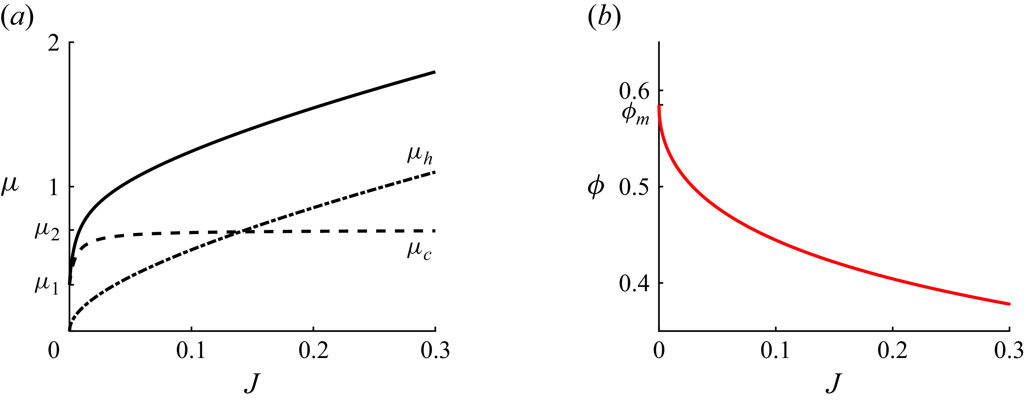
 a
 μ(J)
 b
 ϕ(J)
 a
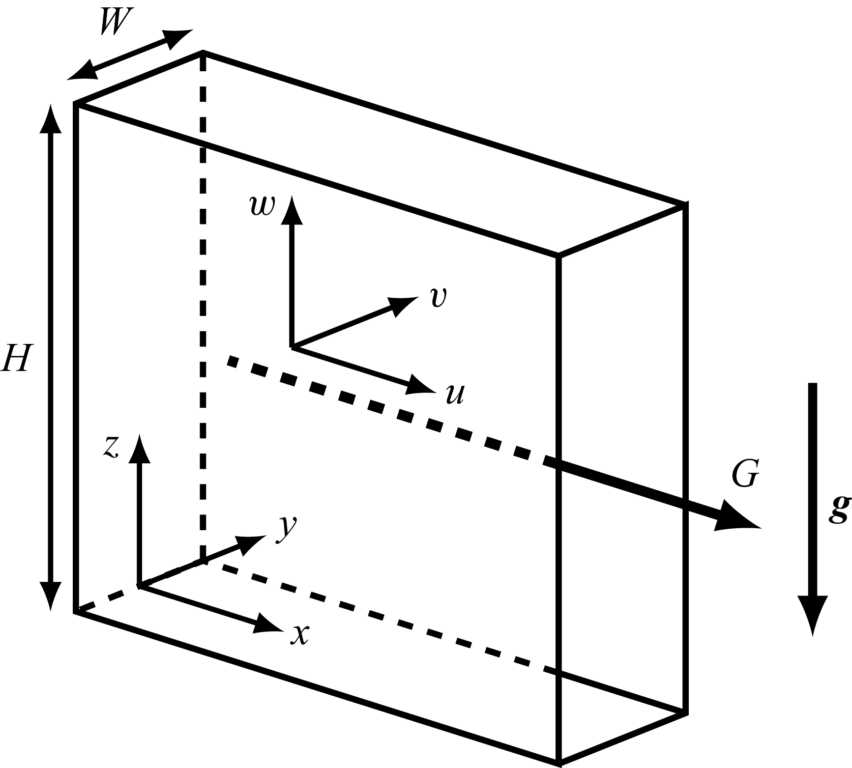
 G
 g
 (u,v,w)
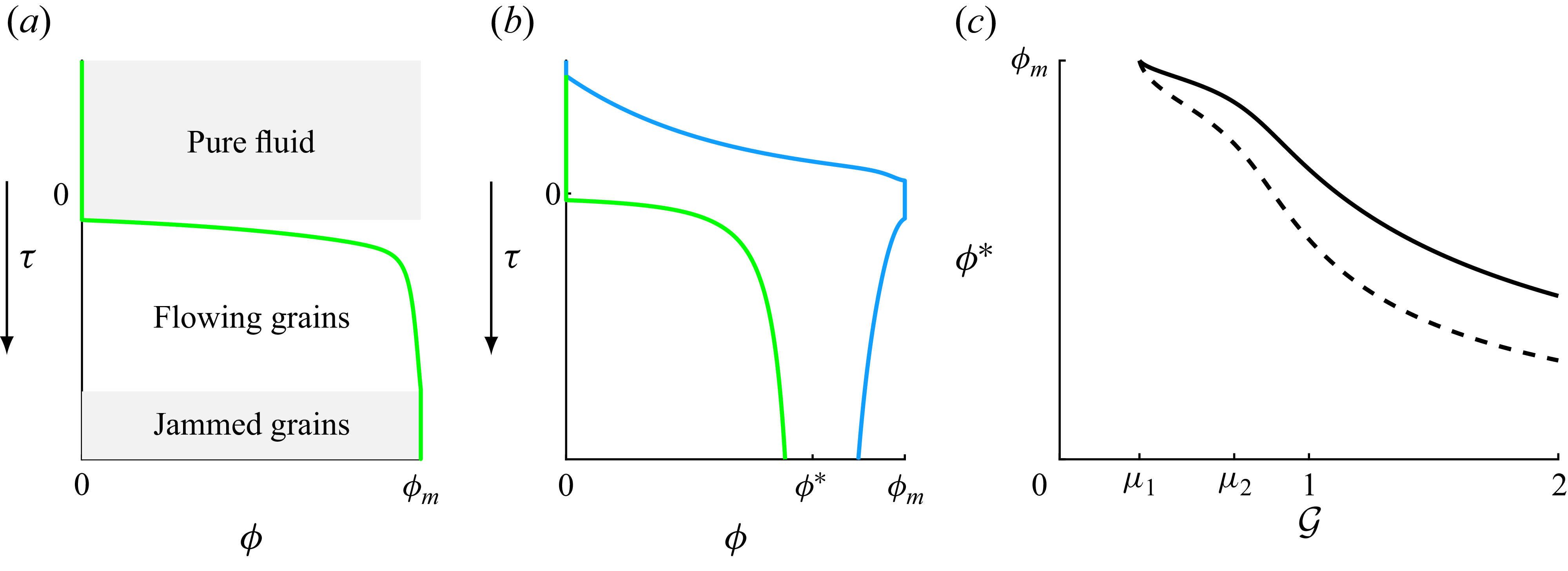
 a
 b
 ϕ
 τ
 z
 a
 G=0.25<μ1
 b
 G=1>μ1
 ϕ<ϕ∗
 ϕ>ϕ∗
 τ>0
 a
 b
 ps(τ=0)
 c
 ϕ∗
 ϕ¯
 G

 a
 z=0,1
 G
 ϕ¯
 ϕ=ϕm
 ϕ(z)
 us
 ϕ
 b
 (G,ϕ¯)=(0.16,0.689ϕm)
 c
 (G,ϕ¯)=(1,0.427ϕm)
 d
 (G,ϕ¯)=(1.5,0.916ϕm)

 a
 Qs
 b
 Qb
 z=0,1
 G
 ϕ¯
 a

 a
 ϕ¯=0.5ϕm
 G
 b
 G=0.01
 ϕ¯
 c
 G=10
 ϕ¯

 a
 z=0,1
 G
 ϕ¯
 a
 μW/ϵ=0,0.1,0.5,1,2
 a
 μW/ϵ
 μW/ϵ
 b
 (G,ϕ¯)=(0.6,0.6ϕm)
 c
 (G,ϕ¯)=(1.08,0.65ϕm)
 d
 (G,ϕ¯)=(1.5,0.77ϕm)

 a
 ϕ
 b
 us
 y=±1/2
 G~=2
 ϕ¯=0.974ϕm

 a
 y=±1/2
 G~
 ϕ¯
 ϕ
 us
 z
 ⟨us⟩y:=∫−1/21/2usdy
 ⟨ϕ⟩y
 b
 (G~,ϕ¯)=(0.5,0.822ϕm)
 c
 (G~,ϕ¯)=(2,0.486ϕm)
 d
 (G~,ϕ¯)=(3,0.786ϕm)

 a
 Qs
 b
 Qb
 y=±1/2
 G~
 ϕ¯
 a

 us
 j
 j
 Qtot
 Qs
 Δpf
 G

 ϕm
 μ1
 μ2
 J0

 a
 Qtot
 Qs
 G
 ×
 Qr
 G
 G=0.538
 G
 G
 Qs
 7%
 6%
 Qtot
 b
 F
 Fb
 ϕm=0.579
 Qtot

 a
 G
 Qs
 Qtot
 G
 μW/ϵ
 Qtot=0.25
 min−1
 Qtot=0.15
 min−1
 Qr=DaG
 G
 Qs
 7%
 6%
 Qtot
 Qs
 G
 b
 a
 Qs
 lW

 us
 a
 f
 g
 k
 a
 us
 μW/ϵ=0,1,2
 Qtot=0.25
 min−1
 a
 f
 Qtot=0.15
 min−1
 g
 k
 us
 8%
 G
 7%

 us
 ⟨us⟩y
 lW=0,1,2
 us
 8%
 G~
 7%
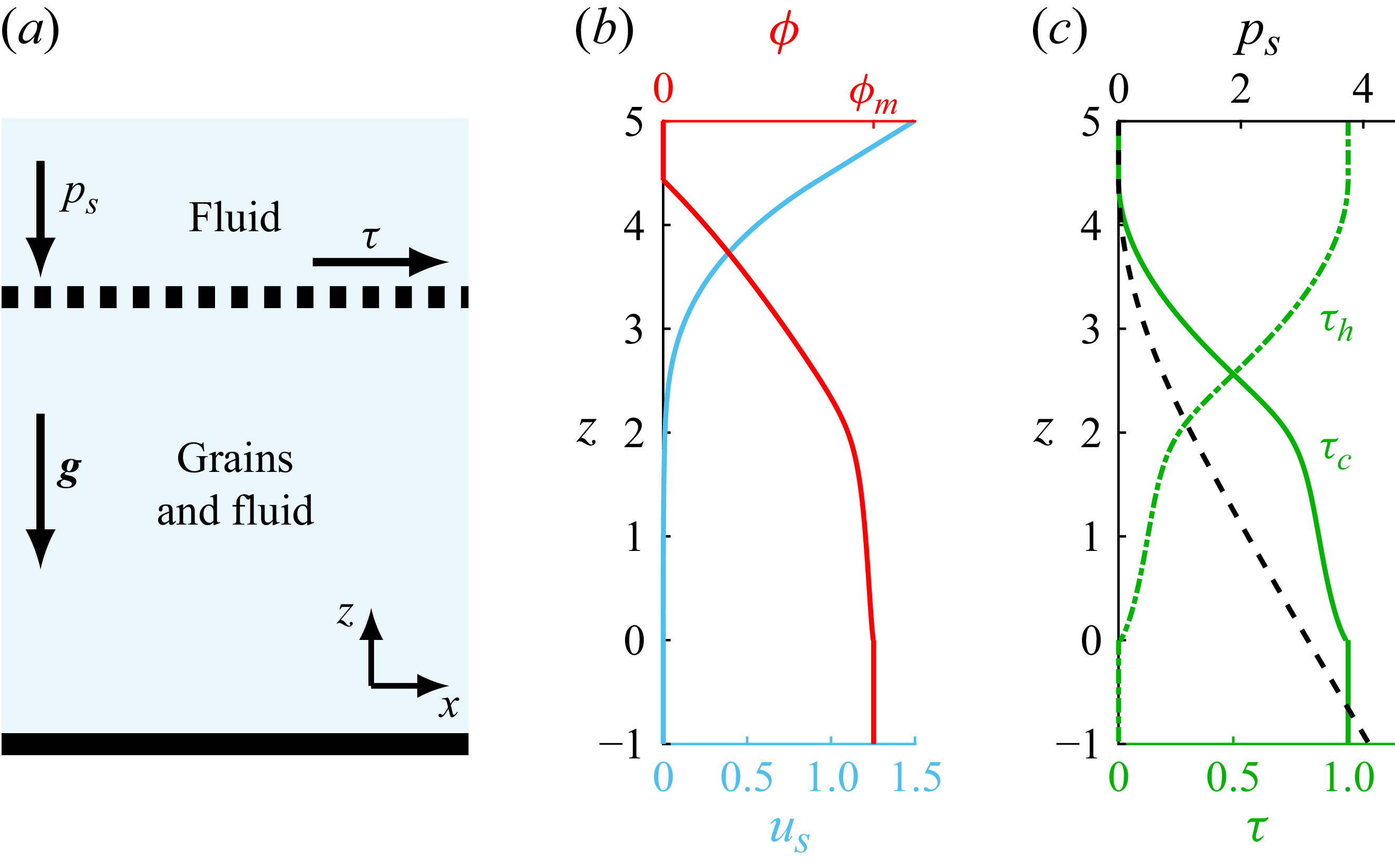
 a
 b
 us
 ϕ
 z
 z=0
 c
 ps
 τ

 a
 ϕ¯=0.5ϕm
 G~
 b
 G~=0.1
 ϕ¯
 c
 G~=100
 ϕ¯

 Open access

