INTRODUCTION
Varian (1982, 1983) described nonparametric methods that can be used to test data for consistency with optimizing models. The most widely applied test is the test of the Generalized Axiom of Revealed Preference (GARP). It has been used to test for utility maximization, as well as to test for weak separability. A defect of all such tests is that they do not incorporate measurement error into the analysis (Varian, 1985). Simulation studies have shown that the problem can be significant. Fleissig and Whitney (2003) showed that data generated from a single utility maximizing agent violated GARP in up to 20% of their trials when the observed quantity data contained uniformly distributed measurement errors in the range of ±5%.1
They considered several different specifications of expenditure shares and price distributions. Looking across all their specifications, with 5% measurement errors, GARP was satisfied between 79.4% and 94% of the time (see Fleissig and Whitney, 2003, p. 137).
Weak separability implies that the marginal rates of substitution between goods in the separable group do not depend on the quantities consumed of goods outside the group. Consequently, demand for goods in the separable group depends only on group expenditure and group prices.
Fleissig and Whitney (2003, p. 138) also calculate the proportion of trials that are consistent with a necessary condition for a subgroup of goods to be weakly separable assuming that the dataset passed GARP. The necessary condition is that the prices and quantities of the subgroup are consistent with GARP. The data satisfied this necessary condition between 74% and 88.7% of the time, with measurement errors in the range ±5%. Nonparametric weak separability tests will, therefore, reject the null much of the time because of measurement errors, given the violation rates for both GARP and the necessary condition.
Varian (1985) introduced a test of optimizing behavior within an explicit stochastic framework that can account for measurement error. His empirical application was based on testing the Weak Axiom of Cost Minimization, but he described how to test GARP. Jones, Dutkowsky, and Elger (2005) applied the methodology to test GARP in an empirical study. De Peretti (2004) derived an alternative test of optimizing behavior that is specific to GARP. For GARP, the two test procedures follow the same logical structure and test the same null hypothesis, albeit in different ways. The null hypothesis of the tests is that the true data satisfy GARP, but the observed data may violate GARP as the result of i.i.d. measurement errors in the quantity data. The tests both follow a two-step logical structure if the observed data violate GARP. First, they use a numerical procedure to adjust the quantity data in order to satisfy utility maximization (referred to, hereafter, as the adjustment procedure). Second, they test the computed adjustments for statistical significance (referred to, hereafter, as the test procedure).4
Various nonstochastic methods have been proposed for assessing the severity of GARP violations. Chalfant and Alston (1988) proposed a measure for two observations that violate the Weak Axiom of Revealed Preference (WARP). Afriat (1967) and Varian (1990) developed an inefficiency index, which measures the “margin of error” in the consumer's optimization needed to eliminate all violations. Gross (1995) describes several additional methods, including the maximum possible violations and the violation rate.
In spite of the similarity in structure, the two tests differ on several key points. First, the adjustment procedures used in the tests are different. In Varian (1985), the adjustment procedure is based on the Afriat inequalities and it adjusts all of the bundles simultaneously. In de Peretti (2004), the bundles are adjusted iteratively in order to satisfy GARP, and not all bundles are adjusted. In addition, expenditure on the adjusted bundles is constrained to equal observed expenditure for all observations in de Peretti (2004) but not in Varian (1985). Second, the test procedures are also different. In Varian (1985), the minimized sum of squared errors computed by the adjustment procedure are less than the true sum of squared measurement errors under the null. If the true measurement errors are assumed to be normally distributed, this result can be used to produce a chi-square test statistic.5
See Epstein and Yatchew (1985) for an alternative test.
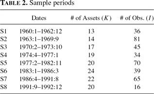
In this paper, we describe the two tests in theoretical terms, highlighting the similarities and differences between them, and then illustrate the two tests in an empirical application. Aggregate monetary asset and user cost data are used in the application, because they often fail to satisfy GARP in empirical studies in contrast to aggregate consumption data. We tested monetary asset stocks and their associated user cost prices for consistency with utility maximization (GARP) using data for the United States from Thornton and Yue (1992). We found GARP violations in seven sample periods, and we implemented the de Peretti and Varian tests in those cases. The sample size and number of assets in each of our sample periods is similar to those in many empirical studies that test monetary asset groupings for weak separability.
Fleissig and Whitney (2003, p. 137) found that measurement errors tended to produce relatively few GARP violations in their simulation study. Consequently, we might expect these two tests to reject the null hypothesis of utility maximization in samples that have large numbers of GARP violations. We were able to directly compare the two tests in six of the seven sample periods. The number of GARP violations were low in five of these six samples and very high in the other sample.6
There were a very high number of GARP violations in the remaining sample, but we were unable to successfully implement the Varian test in that case. We did run the de Peretti test, however, and the results were similar for the two samples with high numbers of GARP violations.
We found that the de Peretti and Varian tests both provided reasonable results and were largely consistent with each other in our application. The tests both supported the null hypothesis of utility maximization in the majority of the five samples that had low numbers of GARP violations. The de Peretti test rejected the null hypothesis in only one of these five samples. We implemented the Varian test using a range of values for the standard deviation of measurement error, because the true value is unknown. We found that we would not be able to reject the null hypothesis in three of the five samples unless we used extremely low values for the standard deviation of measurement errors. In the other two samples, the results were only slightly less supportive.
The de Peretti test strongly rejected the null in the sample that had a large number of GARP violations, which conformed to our expectations. The results for the Varian test indicated that the standard deviation would have to be much higher for this sample than it would have to be for any of the others in order to be unable to reject the null. Thus, the Varian test is much less supportive of the null for this sample than for any of the other samples, which again conformed to our expectations.
The remainder of the article is organized as follows. In Section 2, we describe the two test procedures. In Section 3, we present our empirical application. In Section 4, we conclude.
TEST PROCEDURES
We begin by providing some basic notation and definitions. Let
denote the true unobserved (K×1) vector of quantities of goods consumed in period i∈{1, … , I}. The corresponding (K×1) price vector is denoted by pi=(pi,1, … , pi,K). Let xi =(xi,1, … , xi,K) denote the observed vector of quantities in period i∈{1, …, I}, which possibly contains measurement error.
GARP is defined using standard revealed preference relations. Let P0 denote strictly directly revealed preferred to, R0 denote directly revealed preferred to, and R denote revealed preferred to, see Varian (1982) or de Peretti (2004). The observed dataset violates GARP if xiRxj and xjP0xi for any pair of observations i, j ∈{1, …, I}. A dataset is consistent with utility maximization if and only if it satisfies GARP; see Varian (1982).
Null Hypothesis
The null hypothesis for both the Varian (1985) and de Peretti (2004) tests is that the true unobserved dataset
is consistent with GARP. The observed dataset {xi, pi:i=1, … , I} may or may not satisfy GARP. xi and
are assumed to be related to each other through a random multiplicative term representing measurement error:

where the εi,k are assumed to be zero-mean i.i.d. random variables with variance σ2.
If the observed dataset violates GARP, then the adjustment procedures each calculate a perturbation of the observed quantity data that is consistent with GARP. We use the notation
to denote the (K×1) vector of adjusted quantities in period i∈{1 , …, I} computed by either procedure, which satisfy GARP. Let
denote the computed error of good k in period i defined by (2).

The Varian (1985) Test
In Varian (1985), the adjustment procedure is based on minimizing objective function (3) subject to (4), in
and μi for i∈{1, … , I}.


The Afriat indexes, Vi and μi, are constrained to be strictly positive for all i∈{1 , …, I}. The solution for the
arguments is called the minimal perturbation, which we denote by
for i∈{1 , …, I}. Varian (1982) proved that a dataset satisfies GARP if and only if there exist indexes satisfying the Afriat inequalities (4). Thus, the adjusted dataset
satisfies GARP, by construction. Under the null hypothesis, the true unobserved dataset
also satisfies GARP.
Therefore, under the null, the following property must hold by definition:

If we assume that the true measurement errors, εi,k, are normally distributed i.i.d. random variables with zero mean and variance σ2, then
is distributed as a
. Let Cα be the critical value for a
at the α significance level. A standard hypothesis test would be to reject the null if
. The test statistic cannot be computed, however, because the true data are unobserved. To resolve this problem, Varian (1985) suggested rejecting the null hypothesis if

In applications, the test could be run using an estimate of the true standard deviation; see Varian (1985, p. 449).7
Note that if the observed data actually satisfy GARP, then
by definition.
The de Peretti (2004) Test
In de Peretti (2004), the adjustment procedure is based on minimizing the objective function (3) iteratively using the information contained in the transitive closure matrix. A detailed description of the iterative adjustment procedure is provided in de Peretti (2004). We will focus on highlighting the differences between the de Peretti (2004) and Varian (1985) adjustment procedures. The main differences are that (i) the de Peretti adjustment procedure is iterative, and (ii) the constraints are different.
The de Peretti (2004) adjustment procedure builds on a method for adjusting a particular bundle, xi, which is involved in a GARP violation. The method is to minimize (7) subject to (8), in
.


The constraint (8) can be implemented through (9) and (10):


The adjustment procedure is an iterative algorithm. The iterative algorithm starts at the highest rupture of the preference chain and works downward, adjusting one bundle at each iteration until all violations have been eliminated. The bundle to be adjusted at each iteration is chosen from amongst the subset of bundles, B, involved in the highest remaining rupture of the preference chain. Specifically, (7) is minimized subject to (9) and (10) for all i∈B. The bundle that is adjusted is the one,
, with the smallest minimized value of (7) and the corresponding adjusted quantity,
, is set equal to the optimal solution. The expenditure constraint (9) insures that the adjustment does not produce additional ruptures at higher levels of the preference chain. Each bundle is adjusted at most once.
is set to equal xi for any bundles that were not otherwise adjusted by the procedure. The adjusted dataset satisfies GARP by construction.
The test procedure consists of testing the computed errors for independence and identical distribution. In this paper, we test the time series, st, consisting of the pooled nontrivial computed errors, see de Peretti (2004) for details. We estimate two auxiliary regressions:


where

and test the estimated coefficients of the regressions for joint significance, see Spanos (1999).8
We also could have formulated multivariate tests for independence that explicitly account for the dependence pattern in specific goods.
Discussion
To avoid potential misinterpretation, we begin our discussion by noting that we do not interpret either adjustment procedure as estimating the true data or the true measurement errors.9
See Varian (1985, p. 450–451) for related discussion.
We can now proceed to compare and contrast some particular aspects of the two adjustment procedures. First, the Varian (1985) adjustment procedure should typically result in smaller adjustments, in the least squares sense, than the de Peretti (2004) adjustment procedure. The main reasons for this are that the de Peretti (2004) procedure is iterative and it adjusts the quantities within a particular bundle holding total expenditure fixed. As a result, it eliminates GARP violations by adjusting bundles along the observed budget lines. The quantities of some goods within an adjusted bundle will be adjusted upward and the quantities of others will necessarily be adjusted downward to offset the effect on total expenditure. In Varian (1985), the minimal perturbation is not constrained in terms of expenditure and all bundles are adjusted simultaneously. Therefore, it eliminates GARP violations, in part, by adjusting total expenditure. In this way, expenditure acts as a buffer variable, which allows for smaller adjustments relative to de Peretti's procedure.
The preceding argument is subject to an important caveat, however. The minimal perturbation cannot be computed exactly but must instead be approximated numerically using a nonlinear programming solver. The complexity of the nonlinear programming problem leads to the usual issue of convergence to a local minimum. If the numerical procedure used to approximate the minimal perturbation were to converge to a local minimum, but not to the global minimum, then the de Peretti (2004) procedure could produce a lower total sum of squared adjustments.
Second, the Varian (1985) adjustment procedure is much more time consuming to run than the de Peretti (2004) adjustment procedure. In Varian (1985), the adjustments are computed simultaneously subject to a system of nonlinear inequalities (4). The number of nonlinear inequality constraints is I(I−1), which implies that the computational burden increases substantially as the sample size, I, increases. In addition, the number of adjusted quantities is IK, which implies that the computational burden of the procedure also increases with the number of goods, K. In contrast, the de Peretti (2004) procedure iteratively adjusts the data. The procedure involves repeated minimizations of (7) subject to (9) and (10) for different bundles. The burden of these minimizations does not increase significantly with either sample size or number of goods. Thus, in practice, the de Peretti (2004) procedure runs very quickly, whereas the Varian (1985) procedure can be very time consuming to run (especially, on a large sample).
We now turn to the test procedures. The two tests convey different information because of the different approaches used to test the null hypothesis. Varian (1985) suggests testing if the computed errors (needed to render the data consistent with GARP) are large, in the least-squares sense, given the standard deviation of measurement errors and assuming normality. De Peretti (2004) suggests testing if the computed errors are i.i.d. , assuming that they inherit the i.i.d. property from the true errors, under the null. In effect, Varian suggests looking at the magnitude of the computed errors, whereas de Peretti looks at their distribution. Large computed errors can be i.i.d. and, likewise, small computed errors may not be independent or identically distributed. Thus, the two tests provide different information and are, therefore, likely to be complementary in an empirical study. We now proceed to examine them in an empirical application.
EMPIRICAL APPLICATION
The application is based on testing the underlying data used by Thornton and Yue (1992) to calculate a set of Divisia monetary aggregates for the United States from 1960 to 1992. The data consists of monthly observations of nominal asset stocks and real user costs for the assets in the monetary aggregate L (Liquid Assets). See Barnett (1978, 1980) for derivations of the user cost formula. We converted these data to real per-capita stocks and nominal user costs using the CPI and a measure of population. For reference, the set of monetary assets is detailed in Table 1.

We cannot test the dataset for GARP over the entire sample, 1960–1992, because of inconsistencies in the data. This is mainly because of the introduction of new monetary assets, such as Super NOW accounts, money market deposit accounts, and money market mutual funds.10
The dataset is also inconsistent in some respects with the newer dataset described in Anderson, Jones, and Nesmith (1997).

Fisher and Fleissig (1997, pp. 461–464) divided their dataset (also from Thornton and Yue, 1992) into 21 subsamples of 1960:1–1993:5 and they tested groups of monetary assets (corresponding to M1A, M1, M2, M3, and L) for weak separability over each of them. Weak separability is the key property required for the existence of an economic monetary aggregate, see Barnett (1982), Swofford and Whitney (1994), and Barnett and Serletis (2000). A necessary condition for a group of assets to be weakly separable is that they satisfy GARP. In each of these 21 subsamples, they found that “… there were no violations of GARP for the entire set of data provided by the Federal Reserve.”
Nonstochastic Tests
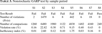
We tested the L monetary assets for GARP in our eight sample periods. We report the nonstochastic GARP test results in Table 3. The L assets violate GARP in all of our sample periods, except for S8. We report the number of GARP violations (nvio), the number of nontrivial binary comparisons I(I-1), the violation rate nvio/I(I-1), and inefficiency indexes for S1–S7.11
Gross (1995) discusses more sophisticated definitions of the violation rate. Varian (1990) defines the Afriat efficiency index. The efficiency index is defined through the relations
and
. The relations are defined as follows:
if epi·xi ≥ pi·xj and
if epi·xi > pi·xj. GARPe is defined (using these relations) analogously to GARP. The efficiency index is the largest number, e*, between 0 and 1, such that the data is consistent with GARP
. We report the inefficiency index as a percentage, 100(1−e*), in Table 3.

S2 and S5 have extremely high numbers of GARP violations, 1479 and 442 respectively, with corresponding violation rates of 23% and 9%. We also computed the number of GARP violations recursively from observation 1 to i, for i=2, …, I. For S2 (I=81), we found no violations up to i=45, but rapid increases in violations thereafter. For S5 (I=70), we found no violations up to i=41, and only a moderate number of violations up until i=64. The high number of violations suggests that the rejection of GARP is probably not attributable to measurement errors in either S2 or S5, see Fleissig and Whitney (2003, p. 137).
We ran the two tests outlined in Section 2 over the L assets for S1–S7. We will refer to S1, S3, S4, S6, and S7 collectively as Group 1, and we will refer to S2 and S5 as Group 2. In the next two sections, we present results for the two tests. The two tests were run separately, one by each author. de Peretti ran his test and Jones ran the Varian test.12
The test results were analyzed separately and then reported to the other author. The interpretations of the results were, however, written jointly.
The Varian (1985) Test
The minimal perturbation was calculated using the computer code from Jones, Dutkowsky, and Elger (2005), which makes use of the commercial solver FFSQP.13
The programs are written in FORTRAN. See Zhou, Tits, and Lawrence (1997) for detailed description of FFSQP.
Specifically, the solver was unable to find a feasible point for the constraints in S2.
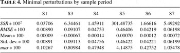
In Table 4, we report results for the minimal perturbation. We report the sum of squared adjustments (SSR) given by (4) multiplied by 1002 , RMSE
multiplied by 100, and descriptive statistics for the computed errors multiplied by 100. The descriptive statistics include the mean, standard deviation, and the maximal absolute value of the computed errors (max).15
That is, max=maxi=1,…,I: k=1,…,K
.

In Group 1, the computed errors are small. For S1, they are bounded by ±0.11%. In S4 and S6, they are bounded by ±0.48% and ±0.43%, respectively. The computed errors are slightly larger in S3 and S7, but S7 is the only sample in Group 1 with any computed errors over 1% in absolute value. In contrast, the computed errors are much larger for S5, which had some errors that were over 4% in absolute value.
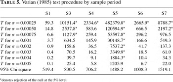
We now turn to the test procedure. The standard deviation of measurement errors, σ, is required in order to implement the test, see (6). Because the true standard deviation is unknown, we ran the test using a range of different values for σ to show how it affects the results. In particular, we ran the test using σ=0.00025 (0.025%), 0.0005 (0.05%), 0.00075 (0.075%), and 0.001–0.005 (0.1–0.5%). We present the results of the test in Table 5. We provide the value of the test statistic, T, defined by (6) as well as the values of the appropriate chi-square distribution at the 95% level.16
We did not compute p-values, because the computed errors are unlikely to be normally distributed.

We first consider the test results for Group 1. If the standard deviation of measurement errors in the data is at least 0.1% (i.e., if σ ≥ 0.001), we would be unable to reject the null hypothesis in any sample in Group 1. If it is 0.075% (i.e., if σ=0.00075), we would only reject for S3. If it is 0.05%, we would only reject for S3 and S7. Although, we do not know the true standard deviation of measurement errors in the data, the test results indicate that our confidence in the observed data would have to be quite high to consider rejecting the null hypothesis in S1, S4, or S6.17
The results for S1 are particularly strong. Even if the standard deviation of measurement errors is as low as 0.025%, we would still not be able to reject the null for S1.
The results are much less supportive of the null hypothesis in S5 than for any sample in Group 1. Specifically, if the standard deviation of measurement error in the data is 0.5% we would be unable to reject the null hypothesis. We would, however, reject the null if the standard deviation is 0.4% or lower.18
It is easy to determine that σ=0.0045 (or 0.45%) is the approximate value where the accept/reject result changes.
The de Peretti (2004) Test
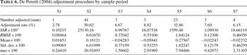
In Table 6, we report results for the computed errors from the de Peretti (2004) adjustment procedure.19
All programs were written using SAS/IML language.
, and descriptive statistics for the nontrivial adjustments. The adjustment procedure found a solution in all sample periods and was very fast.

Given the findings in Table 3, we might expect relatively small computed errors for the samples in Group 1 and relatively large errors for the samples in Group 2, which is exactly what we found. For Group 1, the smallest RMSE is for S1, consistent with much of our previous discussion. The largest RMSE in Group 1 is for S4. Only a few bundles are adjusted by the procedure in each of these samples. For S1, only one bundle is adjusted, whereas for S7, all 18 GARP violations are eliminated by adjusting only 4 bundles (adjustment rate of 6.15%). The results are very different for Group 2. The RMSE for S2 and S5 are much larger than for any Group 1 sample. The number of adjusted bundles was also much larger with adjustment rates of 50.62% for S2 and 32.86% for S5.
The descriptive statistics for each group show a similar pattern. For Group 1, the maximal absolute errors do not exceed 2.32% for any sample. The computed errors in Group 1 are very small relative to those in Group 2. For Group 2, the errors are bounded by ±26.93% for S2 and ±7.95% for S5, indicating that highly nontrivial adjustments in the observed data are needed in order to satisfy utility maximization.
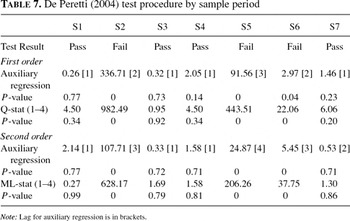
In Table 7, we present the results of the i.i.d. tests. We provide F-tests for the hypothesis that all of the coefficients of the auxiliary regressions (11) and (12) are jointly zero. In addition, we provide the Ljung-Box Q-statistic for first-order independence and the McLeod and Li ML statistic for second-order independence. The tests are performed using the pooled nontrivial computed errors.

For the samples S1, S3, S4, and S7, the null hypothesis cannot be rejected, meaning that the computed adjustments are independent and identically distributed, and the GARP violations should not be considered significant. Utility maximization is, therefore, accepted in these samples. For S2 and S5, the i.i.d. property is strongly rejected by all tests. Maximization is, therefore, rejected for both samples in Group 2. Interestingly, the utility maximization hypothesis is also rejected for S6.
We note that the number of GARP violations is systematically related to the number of adjusted bundles, with larger numbers of violations being associated with a higher adjustment rate. A consequence of this is that the auxiliary regressions are estimated with many more observations for S2 and S5 than for the other samples. The issue is particularly relevant to S1, where only one bundle was adjusted.
Comparison
We begin by comparing the results of the adjustment procedures. The computed errors from the procedures differ in two key respects. First, the de Peretti adjustment procedure adjusts a subset of the bundles, whereas the Varian adjustment procedure can (and typically does) adjust all bundles. The percentage of bundles adjusted by the de Peretti procedure was less than 10% for all samples in Group 1, but was larger for the samples in Group 2. Second, in theory, the de Peretti adjustments should have larger sum of squares as previously discussed. The SSR from the de Peretti procedure is higher than for the Varian procedure in all samples, except for S6. The SSR for the two procedures are approximately equal for S3. These results largely conform to our theoretical prediction.
The results from the two test procedures can be compared for six of the seven samples. For Group 1, the null hypothesis cannot be rejected for S1, S3, S4 or S7 using the de Peretti test, but is rejected for S6. The Varian test results are more subjective, because (6) depends on the standard deviation of measurement errors. If we assume that the standard deviation of measurement errors in the data is at least 0.075% then we would be unable to reject the null hypothesis for S1, S4, S6 or S7. For the remaining sample in Group 1, S3, we would reject the null if the standard deviation of measurement error were 0.075%, but we would be unable to reject if it were 0.1%. The Varian test is slightly less supportive for S3 than for the other samples, but our level of confidence in the observed data would have to be fairly high to consider the rejections significant in any of these five samples. We conclude that the results of the two tests are fairly consistent in Group 1. The main discrepancy between the results (in Group 1) is in regard to S6, where the de Peretti test rejected the null.
The results for S6 are interesting, because the number of GARP violations is low, the SSR obtained by both adjustment procedures is low, and the computed errors produced by both procedures are small. Nevertheless, the de Peretti test rejects in this sample, because the computed errors from the corresponding adjustment procedure are found to violate independence. The results for this sample underscore the differences in the decision rules of the two tests.
For Group 2, we were unable to compare results for S2, because we could not compute the minimal perturbation for this sample.20
The problem does not appear to be sample size. We speculate that the problem is instead related to the extremely high number of GARP violations. As previously noted, Fleissig and Whitney (2003) found that measurement error did not tend to produce high numbers of GARP violations, which suggests that the problem may not be very important in practice.
CONCLUSIONS
We compared the Varian and de Peretti measurement error tests in theoretical terms and in an empirical application. In the empirical application, we used the two tests to determine if GARP violations were statistically significant for a large set of U.S. monetary assets over multiple sample periods spanning 1960–1992. The tests both supported the null hypothesis of utility maximization in the majority of the samples that had low numbers of GARP violations, although there were some discrepancies between them. The tests also could be directly compared in one sample that had a large number of GARP violations. The de Peretti test rejected the null in that sample and the Varian test was much less supportive of the null than it was in any of the other samples. The results from the two tests were, therefore, largely consistent with each other and conformed to our expectations, which were based on available Monte Carlo evidence. We suggest that researchers should consider using both tests in empirical studies until more extensive comparative results become available. These tests can both be run on datasets with reasonable sample sizes and numbers of goods, although the Varian test is much more time consuming to run.
Barnett and Choi (1989) evaluated both parametric and nonparametric weak separability tests in an extensive simulation study. They found that “[r]elative to the separability testing criterion, all models usually did poorly” and that “… the problem is not solved by conducting the test at a point, rather than globally, or by the use of Varian's nonparametric [weak separability] test.” A promising direction for future research may be to incorporate measurement errors into nonparametric tests of weak separability. See Swofford and Whitney (1994, p. 248) for some supportive comments along these lines.
GARP is often tested in connection with testing for weak separability. In particular, Varian (1983) proposed a nonparametric test for weak separability based on a sequence of GARP tests, which has been widely used. The tests in this article can be used to determine if violations of GARP could have been caused by measurement errors in the observed data. The adjusted data produced by either of the two tests satisfies GARP and could, therefore, be used in subsequent tests or estimations that require GARP (see Varian, 1985, p. 449, for more general comments along the same lines). For example, Jones, Dutkowsky, and Elger (2005) calculated adjusted data using the Varian (1985) procedure, which they used in subsequent weak separability tests. A more sophisticated approach would be to generalize the measurement error approaches described in this article to test violations of weak separability for significance. See, for example, de Peretti (2005a) for a weak separability test within an explicit stochastic framework.
Another direction for future research is to compare the two test procedures in a formal simulation study. De Peretti (2005) provides simulation results for his test, but there are no comparable results available (that we are aware of) for the Varian (1985) test. The computational burden of the Varian (1985) adjustment procedure is, however, a limiting factor at present. In addition, the results of the Varian test depend on the measurement error variance specified by the tester.
ACKNOWLEDGMENTS
The content of this joint article is based on a comment and reply to de Peretti (2004). We thank William Barnett for suggesting that we write a joint article, or “exchange,” synthesizing our views. We thank Dan Thornton for a helpful discussion regarding the dataset used in this paper. We also thank Bob Rasche for providing us with historical monetary data, which we used in an earlier draft. We thank Don Dutkowsky, David Edgerton, Thomas Elger, and Chris Hanes for helpful comments and discussions.
Barry Jones was a visitor at Syracuse University when this paper was written. He thanks the Department of Economics at Syracuse University and the Department of Economics at Lund University for helpful comments in seminars. He also thanks AEM Design for providing FFSQP and the Jan Wallander and Tom Hedelius Foundation (Grant J03/19) for financial support.
All interpretations are the responsibility of the authors.