

1 Introduction
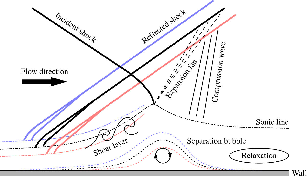
The presence of shock and turbulent boundary layer in the vicinity of the wall in a supersonic flow results in an interaction region where the two meet. The interaction leads to an extensive modification of the boundary layer immediately downstream of the shock, resulting in the boundary layer being in a non-equilibrium state where strong gradients exist in the streamwise direction. Such interactions occur in a number of external and internal flows in aerospace applications, and thus need to be carefully considered when designing components such as airframes and turbomachinery. A schematic of the shock wave boundary layer interaction (SWBLI) when an oblique shock impinges on a boundary layer is given in figure 1. For this shock reflection configuration, the thickening of the boundary layer from interactions with the incident shock leads to the bending of the streamlines in the supersonic region, resulting in the generation of a reflected shock upstream of the incident shock foot. Thus, two interaction sites exist for this configuration, since the reflected shock also interacts with the boundary layer. Note that other configurations, such as compression ramp, also lead to curvature of the supersonic streamlines and generation of a shock in the vicinity of the wall. The thickening of the boundary layer can also lead to flow reversal in the vicinity of the wall and the formation of a separation bubble downstream of the generated shock. The shock reflection configuration occurs commonly when supersonic flow travels through a duct with opposing sidewalls and is typically accompanied by a series of subsequent reflections as the reflected shock from one wall impinges on the opposing wall to form a shock train. The duct flows are ubiquitous in engineering applications, and therefore the ability to accurately predict the resulting SWBLI has enormous practical relevance. Despite the high practical relevance, investigations of the shock reflection configuration remain smaller in scope compared to the compression ramp configuration (Settles & Dodson Reference Settles and Dodson1994a,Reference Settles and Dodsonb; Pirozzoli & Grasso Reference Pirozzoli and Grasso2006). Furthermore, Pirozzoli & Grasso (Reference Pirozzoli and Grasso2006) suggest that the shock reflection configuration is better suited to examining SWBLI since the effect of bulk flow compression is isolated and therefore the effects from concave streamline curvature, which can introduce turbulence amplification and formation of large-scale structure due to a Görtler-like instability mechanism (Spall & Malik Reference Spall and Malik1989; Ren & Fu Reference Ren and Fu2015), are reduced compared to the compression ramp configuration. Hence, the shock reflection configuration is chosen for the current study.
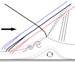
Schematic of an oblique shock boundary layer interaction. The thick solid, dash-dotted and dotted lines correspond to the shock, sonic line and edge of the separation bubble. The mean position is shown in black while instances when the incoming boundary layer thickness is low (high-momentum event) or high (low-momentum event) are indicated with red and blue colours, respectively. Note that, the deviations in the sonic line, expansion fan and compression wave downstream of the interaction region for the low- and high-momentum events have been omitted. Figure adapted from Touber & Sandham (Reference Touber and Sandham2009).

One of the notable features of SWBLI is the oscillatory nature of the shock generated in the vicinity of the wall (see figure 8 for an example). The shock in extreme cases can oscillate several boundary layer thicknesses about the mean position (Thomas, Putnam & Chu Reference Thomas, Putnam and Chu1994). This can lead to an elevated surface pressure fluctuation level and instantaneous shock structures that are vastly different from the time-averaged structure (Muck, Bogdonoff & Dussauge Reference Muck, Bogdonoff and Dussauge1985). The resulting unsteadiness, if strong enough, may lead to a catastrophic failure, e.g. structural damage in a supersonic vehicle. Analysis of the reflected shock location and the size of the separation bubble by Piponniau et al. (Reference Piponniau, Dussauge, Debieve and Dupont2009) in a shock reflection configuration showed that the reflected shock movement closely follows the expansion–contraction cycle exhibited by the separation bubble. A similar conclusion is reached by Grilli et al. (Reference Grilli, Schmid, Hickel and Adams2012), who also investigated the shock reflection configuration using large eddy simulation (LES). Furthermore, the strong correlation between the shock location and the separation/reattachment location at low frequencies is also observed in the compression ramp configuration (Priebe & Martín Reference Priebe and Martín2012), and therefore a general consensus is that the shock oscillation is driven by the expansion and contraction of the separation bubble that forms downstream of the interaction region. However, despite multiple investigations examining SWBLI, the community remains largely divided between two main schools of thought on why the separation bubble exhibits low-frequency unsteadiness.
On one side, Beresh, Clemens & Dolling (Reference Beresh, Clemens and Dolling2002) and Ganapathisubramani, Clemens & Dolling (Reference Ganapathisubramani, Clemens and Dolling2007) associate the low-frequency unsteadiness with a passage of very long coherent structures with a streamwise length of approximately 50 boundary layer thicknesses over the interaction region. They proposed that the very-large-scale low- and high-momentum structures interact differently with the shock, due to a fuller profile associated with the high-momentum region being better able to negotiate the adverse pressure region compared to the low-momentum region and hence resulting in contraction of the separation bubble at that instance. Furthermore, the high-momentum regions are typically flanked by low-momentum regions in the spanwise direction (Hutchins et al. Reference Hutchins, Monty, Ganapathisubramani, Ng and Marusic2011), giving rise to a streamwise translation of the upstream extent of the separation bubble as a function of the spanwise location, resulting in spanwise rippling patterns in the reflected shock (Humble et al. Reference Humble, Elsinga, Scarano and Van Oudheusden2009).
An alternative argument put forward by Dupont, Haddad & Debieve (Reference Dupont, Haddad and Debieve2006) and Piponniau et al. (Reference Piponniau, Dussauge, Debieve and Dupont2009) associates the low-frequency unsteadiness with the formation of a mixing layer downstream of the reflected shock, which modulates the successive expansion and contraction of the separation bubble, with a minimal influence from the incoming turbulent boundary layer on the interaction region. Linear stability analysis conducted on the mean fields of SWBLI shows that the dominant reflected shock foot oscillation frequency is consistent with the unstable global mode, where the characteristic time scale is orders of magnitude slower than the modes associated with the turbulent structures (Touber & Sandham Reference Touber and Sandham2009; Pirozzoli et al. Reference Pirozzoli, Larsson, Nichols, Bernardini, Morgan and Lele2010). In fact, Touber & Sandham (Reference Touber and Sandham2009) did not observe any turbulent structures that extend for 75 boundary layer thicknesses in the streamwise direction in their LES, which matches with the dominant frequency observed for the reflected shock foot oscillations. This led them to conclude that the incoming flow is unlikely to be directly responsible for the shock oscillation. Thus, the physical mechanisms responsible for the shock oscillation remain a contentious issue, where results from different researchers seem to advocate either one of the arguments.
In an effort to reconcile the seemingly mutually exclusive observations from different researchers, Piponniau et al. (Reference Piponniau, Dussauge, Debieve and Dupont2009) and Clemens & Narayanaswamy (Reference Clemens and Narayanaswamy2014) have proposed that both the upstream and downstream mechanisms may exist to a varying degree. They further proposed that a complex interaction occurs between the two depending on the flow configuration and that the different observations may have simply corresponded to the two extreme cases where one of the mechanisms dominates. For example, Piponniau et al. (Reference Piponniau, Dussauge, Debieve and Dupont2009) proposed that the influence of the incoming boundary layer observed by Beresh et al. (Reference Beresh, Clemens and Dolling2002) and Ganapathisubramani et al. (Reference Ganapathisubramani, Clemens and Dolling2007) may correspond to incipient cases with no or very small region of mean flow separation and that their mixing layer model becomes the dominant mechanism as the occurrence of instantaneous flow separation increases sufficiently to observe a distinct mean flow separation. Although Piponniau et al. (Reference Piponniau, Dussauge, Debieve and Dupont2009) find that the dominant frequency of the shock oscillation decreases by two orders of magnitude when a mean flow separation can be observed compared to the incipient cases, the physical mechanism that governs the behaviour of the dominant shock oscillation frequency remains to be fully understood and the conjecture needs further experimental evidence.
Another source of discrepancy, at least from the experimental point of view, is that the majority of the seminal works are based on a single point measurement of velocity/pressure or shadowgraph/schlieren visualisation. Hence, it is possible that the limited nature of these techniques may have led to contrasting conclusions from different researchers. More recently, development of the particle image velocimetry (PIV) technique has allowed access to the two- and three-dimensional velocity fields and therefore enabled a more detailed examination of the SWBLI processes (e.g. Humble et al. Reference Humble, Elsinga, Scarano and Van Oudheusden2009; Piponniau et al. Reference Piponniau, Dussauge, Debieve and Dupont2009). The current study also utilises the PIV technique to capture the shock and the surrounding velocity field simultaneously, thereby allowing the relevant flow physics to be directly quantified. Sections 2 and 3 detail the experiment and the characteristics of the incoming boundary layer before the shock, respectively. Section 4 re-examines the relationship between the turbulent features residing in the boundary layer and the shock location, based on the instantaneous velocity snapshots and the shock positions. Furthermore, concurrent measurements of the wall pressure are also undertaken to characterise the frequency contents of the shock oscillation. These results are presented in § 5, and the conclusions made by past researchers are reinterpreted with the aid of a significantly richer dataset. In § 6, spanwise characteristics of the oscillating shock and its interaction with the boundary layer are determined, while the summary and conclusions are provided in § 7.
2 Experimental set-up
The experiments are performed in the Trisonic Wind tunnel Munich (TWM) at the Bundeswehr University Munich. This is a blow-down type wind tunnel with a test section measuring  $1800~\text{mm}\times 300~\text{mm}\times 675~\text{mm}$ along the length, width and height, respectively. An integrated system consisting of an adjustable Laval nozzle and diffuser allows for a stable operation across subsonic, transonic and supersonic regimes, with the Mach number ranging from 0.3 to 3.0. Moreover, the free-stream turbulence intensity varies from 1.9 % to 0.45 % (a decrease in the turbulence level occurs with an increasing Mach number) within the operating range of the wind tunnel (Scharnowski, Bross & Kähler Reference Scharnowski, Bross and Kähler2019). The facility has two holding tanks that can be pressurised up to 2 MPa above ambient pressure, holding a combined volume of 356 m3 of dry air. This enables measurement times of the order of 100 s for a typical experiment run. The facility is designed to allow the Reynolds number to be independently controlled from the Mach number by changing the mean stagnation pressure,
 $P_{0}$. The free-stream fluid parameters for the current study are outlined in table 1. Here,
 $M_{\infty }$,
 $U_{\infty }$ and
 $\unicode[STIX]{x1D70C}_{\infty }$ correspond to the mean Mach number, mean streamwise velocity and mean fluid density in the free-stream region upstream of the shock, while
 $T_{0}$ denotes the mean stagnation temperature.
Experiment free-stream parameters.

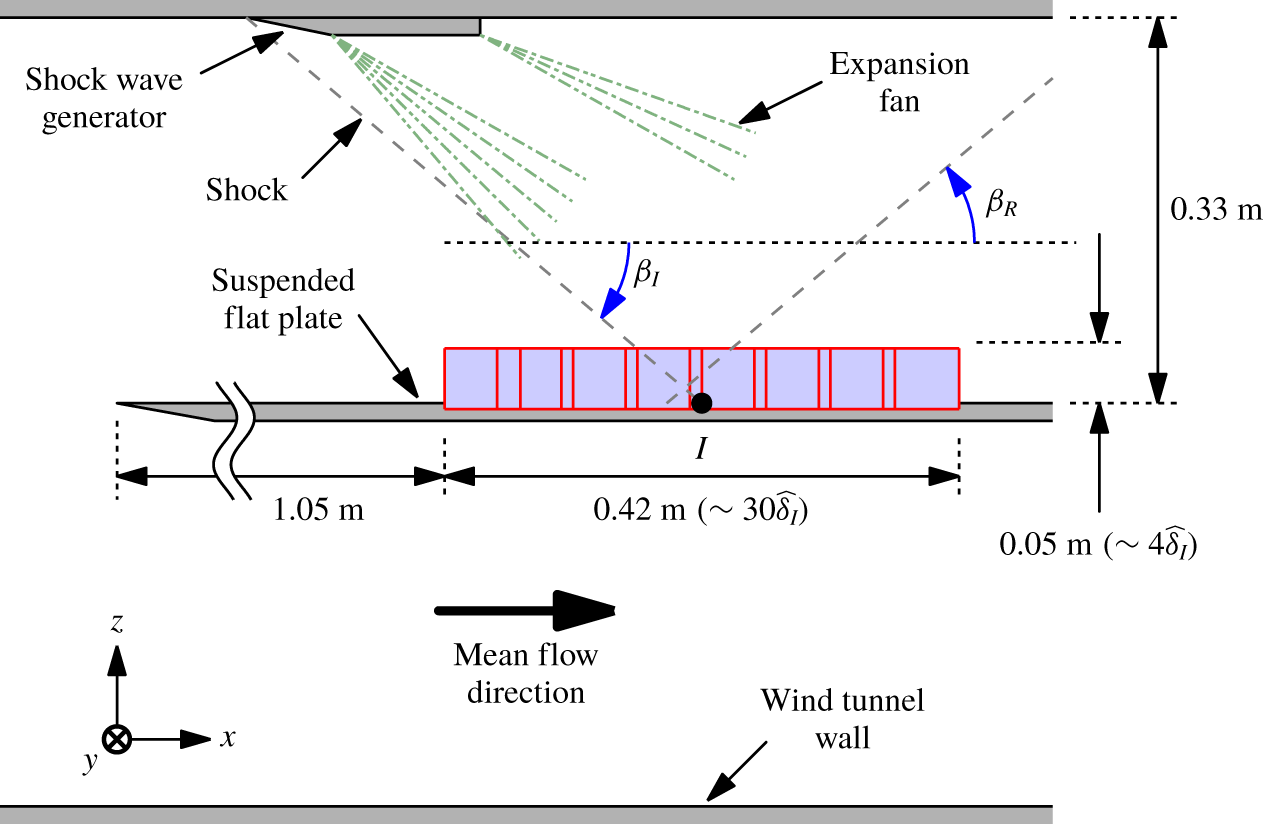
A flat plate, suspended at the middle of the test section, is used to examine the boundary layer that forms in the vicinity of the plate surface. The top and bottom walls have a divergence of  $\pm 0.4^{\circ }$ with respect to the test section centreline to account for the growth of the boundary layer over the walls of the test section and suspended plate. The incident shock is generated by a shock wave generator in the form of a two-dimensional wedge fixed to the upper wall of the wind tunnel, as illustrated in figure 2. The shock generator has a wedge angle of
 $12^{\circ }$, and therefore has an effective angle of
 $11.6^{\circ }$ with respect to the free-stream flow direction. The passage of supersonic flow around the wedge leads to an oblique shock that impinges on the boundary layer developing along the flat plate at a downstream location, and the location of the incident shock foot is denoted here as
 $I$. The leading edge of the shock wave generator is located 390 mm upstream from the mean incident shock foot location,
 $X_{I}$, and, due to the shock wave generator geometry, two expansion fans are generated 75 and 200 mm downstream from the leading edge, as indicated in figure 2. Note that, while the downstream expansion fan resides outside the current field of view (FOV), the upstream expansion fan interacts with the incident shock. This leads to a weakening of the shock which impinges on the flat plate, with a mean incidence angle of
 $\overline{\unicode[STIX]{x1D6FD}_{I}}=36.1^{\circ }$ (based on a linear fit of the
 $\text{d}\widetilde{U}/\text{d}x$ minima in the free-stream region within the FOV), in contrast to
 $40.3^{\circ }$ predicted from the inviscid calculations without the expansion fans. Here,
 $U$ indicate the mean streamwise velocity, while
 $x$,
 $y$ and
 $z$ denote the streamwise, spanwise and wall-normal directions. Further, the tilde and overbar operators indicate instantaneous and the mean quantities, while lower cases, except for
 $x$,
 $y$ and
 $z$, denote fluctuations about the mean value. Moreover,
 $\widehat{\unicode[STIX]{x1D6FF}}_{I}=14~\text{mm}$ (Bross, Scharnowski & Kähler Reference Bross, Scharnowski and Kähler2019b) corresponds to the wall distance at
 $X_{I}$ where the mean velocity is equal to 99 % of the incoming free-stream velocity,
 $U_{\infty }$, for the reference case of a zero-pressure-gradient compressible boundary layer at a matched Mach number (i.e. without the presence of an incident or reflected shock).
A sketch of the experimental set-up. The dashed lines indicate the location of the incident and reflected shock waves, while the blue shaded region shows the combined view from eight cameras (the field of view from each camera is denoted with a red box).  $\unicode[STIX]{x1D6FD}_{I}$ and
 $\unicode[STIX]{x1D6FD}_{R}$ correspond to the angle of the incident and reflected shock relative to the streamwise direction.

2.1 Schlieren visualisations
A schlieren system is utilised to examine the temporal shock location characteristics up to 12.5 kHz. A 1.6 kW Xenon lamp light source is directed towards a slit aperture, located at the focus of a spherical concave mirror with a focal length of 4 m, and the schlieren system is configured to follow a classical Z set-up (Hampel Reference Hampel1984). The long focal length ensures that a high degree of parallelism is maintained between the light rays travelling through the test section. On the other side of the test section, the light rays are collected by a second spherical concave mirror and a knife edge is placed at the focal point. The slit and knife edge are oriented such that variation in the schlieren image light intensity corresponds to the density variation in the wall-normal direction. Furthermore, the knife edge is adjusted such that a good contrast is achieved between the regions with weak and strong density gradients (i.e. regions further away and in the vicinity of the shock). The schlieren visualisations are recorded using a PCO dimax S4 high-speed camera.
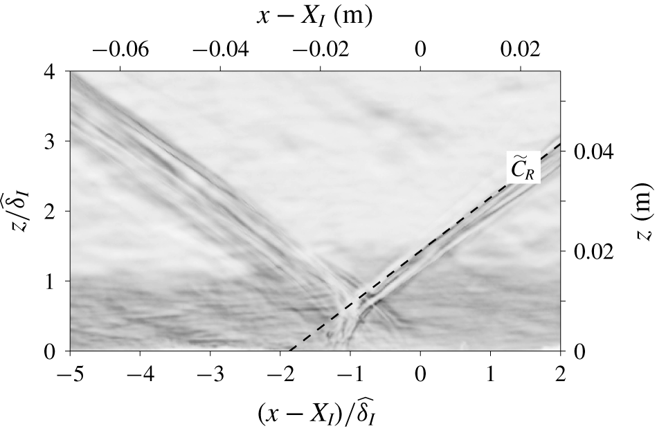
An instantaneous schlieren image of the SWBLI. The dark region corresponds to regions with large magnitude in density gradients (integrated in the spanwise direction) with respect to the wall-normal direction. The dashed line shows the identified reflected shock location,  $\widetilde{C}_{R}$.

Figure 3 shows an instantaneous example of an image used to determine the shock location. Here, the dark region corresponds to regions with large magnitudes in density gradients. The variation in brightness occurs due to the refraction of light from differences in the refractive indices resulting from variation in density. Furthermore, the recorded brightness is a cumulative of the density variation across the spanwise direction, and since the shock location is three-dimensional, exhibiting spanwise rippling patterns (Humble et al. Reference Humble, Elsinga, Scarano and Van Oudheusden2009), it appears as multiple dark bands in the recorded image due to spanwise integration of the intensities. To determine the shock location, the schlieren image corresponding to the free-stream region ( $z/\,\widehat{\unicode[STIX]{x1D6FF}}_{I}>1.4$) is divided into
 $(x-X_{I})/\,\widehat{\unicode[STIX]{x1D6FF}}_{I}\leqslant -1$ and
 $(x-X_{I})/\,\widehat{\unicode[STIX]{x1D6FF}}_{I}>-1$ regions. For each region, a straight line is fitted through dark pixels weighted by the streamwise gradient of the intensity values to capture the most downstream and upstream high-density gradient regions for the incident and reflected shocks, respectively. The identified reflected shock location,
 $\widetilde{C}_{R}$, is shown in figure 3 using a dashed line. Since the shock generator is fixed to the roof of the wind tunnel in the current work (see figure 2), the flow upstream of the shock generator is not uniform in the
 $y$-direction due to the instantaneously varying spanwise distribution of low- and high-momentum features within the boundary layer. Consequently, the incident shock produced by the roof mounted wedge is also three-dimensional. Therefore, unlike for the configuration where the shock generator is placed in the free stream (e.g. Dupont et al. Reference Dupont, Haddad and Debieve2006) and where the incident shock generated is nearly two-dimensional, the incident shock in the current study appears indistinct in the schlieren image shown in figure 3.
2.2 Velocity fields – wall-normal plane
The flow upstream and downstream of the incident shock foot location,  $X_{I}$, is captured using planar PIV. In order to facilitate a large FOV, while still capturing sufficient details of the flow, a multi-camera configuration with eight Imager sCMOS is used, as illustrated in figure 2. This resulted in a combined FOV with dimensions of
 $0.42~\text{m}\times 0.05~\text{m}$ (corresponding to
 $30\,\widehat{\unicode[STIX]{x1D6FF}}_{I}\times 4\,\widehat{\unicode[STIX]{x1D6FF}}_{I}$) in the streamwise and wall-normal directions, respectively, while still maintaining a scaling of
 $25~\unicode[STIX]{x03BC}\text{m}~\text{pixel}^{-1}$. Furthermore, to allow convergence of conditional mean quantities, approximately 4700 statistically independent velocity fields are acquired. It should be noted that, unlike the schlieren visualisations, the illumination for the planar PIV is limited to approximately 1 mm in the spanwise direction. Thus, the instantaneous shock locations are much more well defined (e.g. compare figures 3 and 8), since only a minuscule variation in the shock location occurs over the illuminated spanwise distance for the PIV images. To enable PIV, the flow is illuminated by a double-pulsed laser sheet generated utilising a Quantel EverGreen laser head, rated at
 $200~\text{mJ}~\text{pulse}^{-1}$. The laser sheet is introduced into the test section perpendicularly to the flat-plate wall through an optical glass window installed on the roof of the test section. To minimise regions of high-intensity pixels in the vicinity of the wall, typical in this laser sheet configuration, the aluminium wall surface within the FOV is polished to limit the amount of scattered light and the cameras positioned to be at a similar height as the wall (Kähler, Scharnowski & Cierpka Reference Kähler, Scharnowski and Cierpka2012). In addition, Di-Ethyl-Hexyl-Sebacat (DEHS) tracer particles with a mean diameter of approximately
 $1~\unicode[STIX]{x03BC}\text{m}$ (Kähler, Sammler & Kompenhans Reference Kähler, Sammler and Kompenhans2002) are released into the flow upstream of the settling chamber. The time offset between the double images is set at
 $1~\unicode[STIX]{x03BC}\text{s}$, resulting in a mean particle image shift of 21 pixels in the incoming free-stream region. Note that a large pixel shift is important in reducing the relative uncertainty of the PIV measurements, and results from Scharnowski et al. (Reference Scharnowski, Bross and Kähler2019) suggesting that a mean shift of 20 pixels or more is desirable. The PIV images are processed using Davis 8.3 software from LaVision GMbH, where multi-pass image deformation and Gaussian window weighting are enabled. The initial and final window sizes correspond to
 $128\times 128$ and
 $16\times 16$, respectively, with a 50 % overlap between the windows used for the PIV evaluation.
2.2.1 Fast-response pressure transducers
In addition to velocity fields, which are recorded at approximately 10 Hz, simultaneous wall pressure measurements are acquired at 100 kHz utilising three fast-response Kulite XCQ-062 pressure transducers with a range of  $\pm 350~\text{kPa}$. These transducers are typically able to resolve fluctuating pressure values up to 60 kHz, or approximately one boundary layer turnover time (i.e.
 $U_{\infty }/(f_{U}\,\widehat{\unicode[STIX]{x1D6FF}}_{I})\sim O(1)$, where
 $f_{U}$ denotes the upper bound of the resolvable frequency). The pressure taps are located at a small spanwise offset (
 ${\approx}1~\text{mm}$) to the laser sheet, in order to avoid saturation of camera pixels from the scattered light, and are streamwise aligned. The locations of the pressure transducers
 $\mathtt{P}_{1}$–
 $\mathtt{P}_{3}$ with respect to the mean incident and reflected shock locations are as indicated in figure 4. The fast-response pressure transducers are calibrated by applying a known pressure onto the backside of the membranes via reference tubes connected to a General Electric PACE 5000 pressure controller. The voltages from each pressure transducer are recorded at nine different pressures in the range
 $\pm 70~\text{kPa}$, and a linear fit determined between the pressure and the mean recorded voltage. The linear fit is then utilised to convert the recorded voltage values from the pressure transducer during the measurement to the pressure values. The uncertainty associated with the measured pressure values due to nonlinearity, non-repeatability and hysteresis is expected to be less than
 $\pm 1.8~\text{kPa}$.
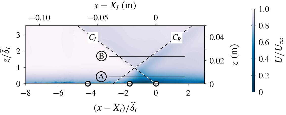
The location of fast-response pressure transducers and wall-parallel PIV planes with respect to the mean incident ( $C_{I}$) and reflected (
 $C_{R}$) shock locations. The colour iso-contours correspond to the mean streamwise velocity field. The pressure transducers
 $\mathtt{P}_{1}$–
 $\mathtt{P}_{3}$ are denoted by ○ symbols and are located at
 $(x-X_{I})/\,\widehat{\unicode[STIX]{x1D6FF}}_{I}\approx -4$,
 $-1.5$ and 0, respectively; while the wall-parallel PIV planes Ⓐ and Ⓑ are at
 $z/\,\widehat{\unicode[STIX]{x1D6FF}}_{I}\approx 0.4$ and 1.7.

2.3 Velocity fields – wall-parallel plane
In addition to the wall-normal PIV plane, wall-parallel measurements are undertaken at  $z/\,\widehat{\unicode[STIX]{x1D6FF}}_{I}\approx 0.4$ and 1.7, as illustrated in figure 4. Both wall-parallel planes are intersected by the incident and reflected shocks, and the planes are configured so that the plane closer to the wall resides within the boundary layer developing over the flat wall, while the plane away from the wall is at the free-stream region. The combined FOV of 0.065 m × 0.16 m (
 $5\,\widehat{\unicode[STIX]{x1D6FF}}_{I}\times 11\,\widehat{\unicode[STIX]{x1D6FF}}_{I}$) in the streamwise and spanwise directions, respectively, with a scaling of
 $400~\unicode[STIX]{x03BC}\text{m}~\text{pixel}^{-1}$ is obtained using two Imager sCMOS cameras. The laser, tracer particles and the PIV software used are the same as that for the wall-normal PIV. The initial and final window sizes are set to
 $64\times 64$ pixels and
 $24\times 24$ pixel, respectively, with an initial constant window shift to account for the mean velocity along the plane (Raffel et al. Reference Raffel, Willert, Scarano, Kähler, Wereley and Kompenhans2018). In addition, the time offset between double images is set at
 $2~\unicode[STIX]{x03BC}\text{s}$, resulting in a mean particle image shift of 26 and 30 pixels for the two wall-parallel planes, while all other settings are kept the same. Unlike the wall-normal plane PIV, a mirror-like surface is undesirable for the wall-parallel plane PIV, in terms of minimising the scattered light captured by the camera. Hence, the pressure tap ports were covered and the wall surface painted matt black. Consequently, the wall pressure signals are not available for the current wall-parallel PIV measurements.
Streamwise–wall-normal view of shock wave boundary layer interaction in a shock reflection configuration. The flow is from left to right and (a) and (b) correspond to the mean and instantaneous streamwise velocity fields.

3 Basic features of data
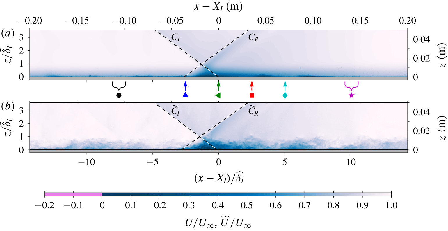
Figure 5(a,b) shows the mean and an instantaneous streamwise velocity fields obtained from the combined FOV for the wall-normal PIV measurement. The large streamwise extent allows for the recovery of the modified boundary layer after the shock to be quantified, while capturing the  $2\,\widehat{\unicode[STIX]{x1D6FF}}_{I}$ region of the free stream allows the instantaneous shock locations to be determined (shown in figure 5 as the dashed lines). In addition to the instantaneous shock location, turbulent features within the boundary layer are simultaneously captured, thus providing a unique dataset where interaction between the turbulent features and the shock can be analysed directly. It should be noted that the current configuration is optimised to capture the outer region of the boundary layer (
 $z/\widehat{\unicode[STIX]{x1D6FF}}\gtrsim 10^{-2}$) since the very-large-scale structures and the mixing layer identified as a possible source of the reflection shock unsteadiness by the past researchers (see § 1 for further details) are thought to reside in this region. However, this means that the chosen configuration is not best suited for evaluation of velocity vectors in the near-wall region where a presence of strong light scatter, low seeding density and strong shear not encountered in the outer region can exist (Theunissen, Scarano & Riethmuller Reference Theunissen, Scarano and Riethmuller2008; Kähler et al. Reference Kähler, Scharnowski and Cierpka2012). This can increase the likelihood of spurious velocity vector evaluation, which can lead to erroneous statistics in the near-wall region.
Despite instances with a reverse flow accounting for approximately 40 % of the total dataset, since the position where the flow separates varies in time, the mean field is found not to contain any separation region, as evident from figure 5(a). Therefore, the current configuration may correspond to an incipient separation case, according to Piponniau et al. (Reference Piponniau, Dussauge, Debieve and Dupont2009). Although Clemens & Narayanaswamy (Reference Clemens and Narayanaswamy2014) caution the use of PIV velocity fields to classify the separation strength since the PIV technique can suppress the reverse flow region due to an inadequate spatial resolution and advocate instead the use of surface flow visualisation techniques, it is unlikely to change the classification for the current study. This is because  $(X_{I}-X_{R})/\widehat{\unicode[STIX]{x1D6FF}}\approx 2$ for the current configuration, and since the streamwise offset between the mean incident and reflected shock foot locations,
 $X_{I}-X_{R}$, provides an upper bound for the extent of the separation region,
 $L_{sep}/\widehat{\unicode[STIX]{x1D6FF}}\ll 2$ (where
 $L_{sep}$ corresponds to the streamwise extent of the separation bubble). Therefore, the current configuration falls under the weakly separated case based on the classification by Clemens & Narayanaswamy (Reference Clemens and Narayanaswamy2014).
3.1 Mean and variance profiles
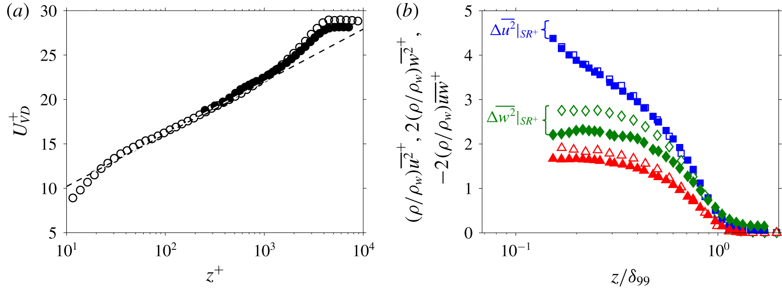
In order to establish whether the boundary layer upstream of the shock is in a canonical state, figure 6(a) shows a comparison between the van Driest (Reference van Driest1951) transformed  $U$ profile at
 $(x-X_{I})/\,\widehat{\unicode[STIX]{x1D6FF}}_{I}\approx -7.5$ from the current work against the incompressible canonical boundary layer profile obtained in the high Reynolds number wind tunnel at the University of Melbourne (Baidya et al. Reference Baidya, Philip, Hutchins, Monty and Marusic2017). The van Driest transformation takes into account the influence of wall-normal gradient in density that arises in the compressible flows, thereby allowing comparisons against the incompressible cases where extensive datasets are available in the literature. Note that the time-averaged density,
 $\unicode[STIX]{x1D70C}(z)$, required for the van Driest transformation is estimated from the mean velocity profile following the temperature–velocity relation of Walz (Reference Walz1959) and the ideal gas law. In order to calculate the mean friction velocity,
 $U_{\unicode[STIX]{x1D70F}}$, the transformed profile is fitted against a composite profile (Chauhan, Monkewitz & Nagib Reference Chauhan, Monkewitz and Nagib2009), as done for the incompressible dataset. In figure 6, superscript ‘+’ is used to denote length (e.g.
 $z^{+}=zU_{\unicode[STIX]{x1D70F}}/\unicode[STIX]{x1D708}_{w}$) and velocity (e.g.
 $U^{+}=U/U_{\unicode[STIX]{x1D70F}}$) scaled by the corresponding viscous scales (where
 $\unicode[STIX]{x1D708}_{w}$ corresponds to the kinematic viscosity of the fluid at the wall). A good agreement observed between the two profiles shown in figure 6(a), indicates that the incoming compressible turbulent boundary layer is in a canonical state.
Figure 6(b) shows comparisons between incompressible and compressible turbulent stress profiles. Note that, here,  $\unicode[STIX]{x1D6FF}_{99}$ corresponds to the
 $z$ location where
 $U=0.99U_{\infty }$ for the
 $U$ profile at
 $(x-X_{I})/\,\widehat{\unicode[STIX]{x1D6FF}}_{I}\approx -7.5$, while the turbulent stress profiles have been pre-multiplied by a factor corresponding to the ratio between the mean density profile and the mean density at the wall,
 $\unicode[STIX]{x1D70C}/\unicode[STIX]{x1D70C}_{w}$, to account for the influence of the wall-normal density gradient in the compressible turbulent boundary layer. Note that, here an additional factor of two is applied to the wall-normal turbulence intensity and the Reynolds shear stress to enhance the readability of the stress values. Furthermore, unlike the mean velocity, the measured turbulent stress profiles are dependent on the spatial resolution of the sensor utilised (Ligrani & Bradshaw Reference Ligrani and Bradshaw1987; Lee et al. Reference Lee, Monty and Hutchins2016). The integration window used for PIV evaluation has dimensions of 130 viscous units × 130 viscous units, while the laser sheet thickness is estimated to be approximately 0.5–1 mm (Grayson et al. Reference Grayson, de Silva, Hutchins and Marusic2018), which corresponds to 150–300 viscous units. In contrast, the incompressible dataset is obtained utilising a cross-wire with dimensions of 13 viscous units × 13 viscous units, with a wire spacing of 7 viscous units. Thus, the turbulent stress profiles from the current study are expected to be more attenuated due to spatial averaging over a larger viscous-scaled dimension compared to the incompressible dataset, as observed for the
 $\overline{w^{2}}$ and
 $\overline{uw}$ profiles. Based on invariance of the small scales when scaled in viscous units, an estimate of the attenuation in
 $\overline{u^{2}}$ and
 $\overline{w^{2}}$ due to mismatched spatial resolution can be obtained (Lee et al. Reference Lee, Monty and Hutchins2016), and the estimated missing energy is indicated by the curly braces at
 $z/\unicode[STIX]{x1D6FF}_{99}\approx 0.15$ (see figure 6b,
 $\unicode[STIX]{x0394}\overline{u^{2}}|_{SR^{+}}$ and
 $\unicode[STIX]{x0394}\overline{w^{2}}|_{SR^{+}}$). The results suggest a slight (
 ${\approx}10\,\%$) overestimation of the
 $\overline{u^{2}}$ statistics and a good agreement of the
 $\overline{w^{2}}$ statistics for the current experiment once the missing energy
 $\unicode[STIX]{x0394}\overline{u^{2}}|_{SR^{+}}$ and
 $\unicode[STIX]{x0394}\overline{w^{2}}|_{SR^{+}}$ are added to account for the finite spatial resolution effects; however, the observed differences are within the experimental uncertainty.
Wall-normal profiles of the (a) first- and (b) second-order moments at  $(x-X_{I})/\,\widehat{\unicode[STIX]{x1D6FF}}_{I}\approx -7.5$ (the streamwise locations contributing to the statistics are shown using curly brace above the ● symbol in figure 5).
 $U_{VD}$ denotes the van Driest transformed
 $U$ profile. Solid symbols: current experiment. Open symbols:
 $Re_{\unicode[STIX]{x1D70F}}\approx 5000$ incompressible canonical turbulent boundary layer data (Baidya et al. Reference Baidya, Philip, Hutchins, Monty and Marusic2017). The symbols represent: ○, ●, mean streamwise velocity (
 $U$); ▫, ▪, streamwise turbulence intensity (
 $\overline{u^{2}}$); ♢, ♦, wall-normal turbulence intensity (
 $\overline{w^{2}}$); and ▵, ▴, Reynolds shear stress (
 $-\overline{uw}$). The
 $\unicode[STIX]{x0394}\overline{u^{2}}|_{SR^{+}}$ and
 $\unicode[STIX]{x0394}\overline{w^{2}}|_{SR^{+}}$ indicate the unresolved missing energy at
 $z/\unicode[STIX]{x1D6FF}_{99}\approx 0.15$ for the current dataset relative to the incompressible dataset due to larger sensor dimensions in viscous units, based on the formulation by Lee et al. (Reference Lee, Monty and Hutchins2016).

Boundary layer parameters upstream of the shock. Here,  ${\mathcal{W}}_{x}$,
 ${\mathcal{W}}_{y}$ and
 ${\mathcal{W}}_{z}$ correspond to the expected spatial resolutions upstream of the shock in the
 $x$,
 $y$ and
 $z$ directions, respectively, based on the PIV window size and the laser thickness.

The mean flow parameters upstream of the shock are summarised in table 2, where  $T_{w}$ corresponds to the temperature at the wall. The momentum thickness is defined as
 $$\begin{eqnarray}\unicode[STIX]{x1D703}=\int _{0}^{\infty }\frac{\unicode[STIX]{x1D70C}}{\unicode[STIX]{x1D70C}_{\infty }}\frac{U}{U_{\infty }}\left(1-\frac{U}{U_{\infty }}\right)\text{d}z,\end{eqnarray}$$
while the friction and momentum thickness Reynolds numbers are given by  $Re_{\unicode[STIX]{x1D70F}}=(\unicode[STIX]{x1D6FF}_{99}U_{\unicode[STIX]{x1D70F}})/\unicode[STIX]{x1D708}_{w}$ and
 $Re_{\unicode[STIX]{x1D703}}=(\unicode[STIX]{x1D703}U_{\infty })/\unicode[STIX]{x1D708}_{w}$, respectively. In compressible flows, an alternative to
 $Re_{\unicode[STIX]{x1D703}}$,
 $Re_{\unicode[STIX]{x1D6FF}_{2}}=(\unicode[STIX]{x1D70C}_{\infty }\unicode[STIX]{x1D703}U_{\infty })/\unicode[STIX]{x1D707}_{w}$, where
 $\unicode[STIX]{x1D707}_{w}$ corresponds to the dynamic viscosity of the fluid at the wall, is more widely cited since the Reynolds number based on the conventional momentum thickness ceases to be an effective specifying parameter for the compressible flows (Fernholz & Finley Reference Fernholz and Finley1980).
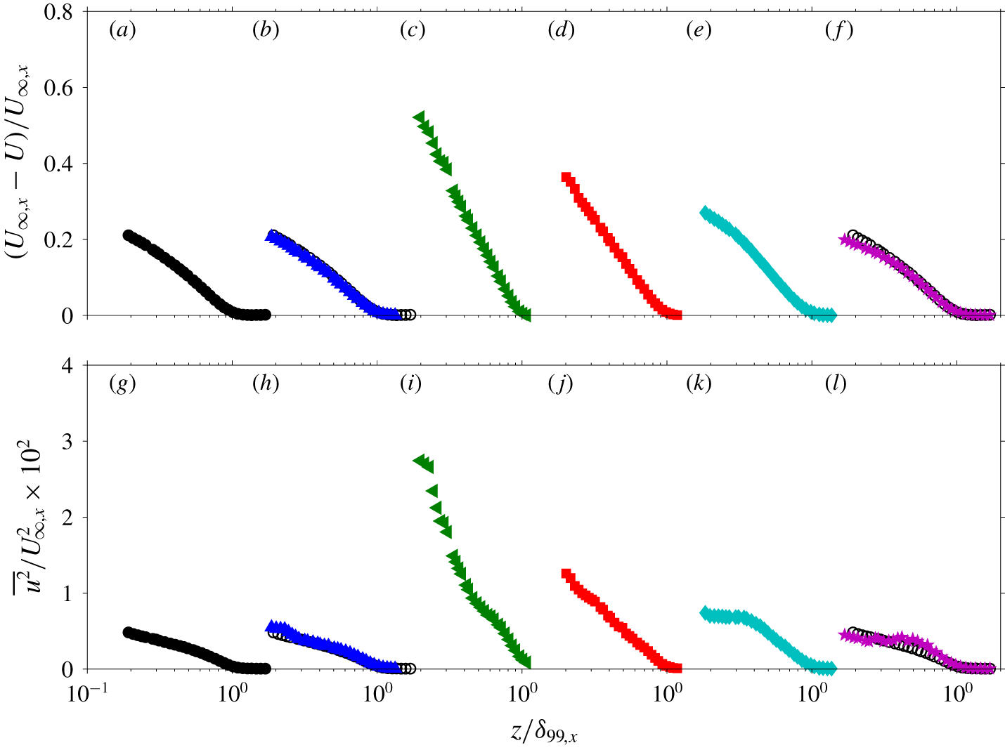
Figures 7(a–f) and 7(g–l) show the streamwise evolution of the velocity deficit ( $U_{\infty }-U$) and the streamwise turbulence intensity (
 $\overline{u^{2}}$), respectively. Note that, for convergence reasons, the profiles at
 $(x-X_{I})/\,\widehat{\unicode[STIX]{x1D6FF}}_{I}=-7.5$ and 10 have been obtained by spatial averaging the velocity vectors that lie within
 $\pm 0.5\,\widehat{\unicode[STIX]{x1D6FF}}_{I}$ in the
 $x$ direction. At far upstream and downstream locations from the shock, the streamwise change in
 $U$ and
 $\overline{u^{2}}$ over one boundary layer thickness is minimal. Thus, by considering the velocity vectors that lie within
 $\pm 0.5\,\widehat{\unicode[STIX]{x1D6FF}}_{I}$, the total number of independent samples used to compute the statistics can be increased, which reduces the uncertainty associated with the computed value. For
 $x$ locations in the vicinity of the shock (i.e.
 $(x-X_{I})/\,\widehat{\unicode[STIX]{x1D6FF}}_{I}=-2.5$, 0, 2.5 and 5), a large change in
 $U$ and
 $\overline{u^{2}}$ can occur over a small
 $x$ displacement and therefore only temporal averaging is performed for these profiles. The profiles are shown normalised by the local boundary layer thickness,
 $\unicode[STIX]{x1D6FF}_{99,x}$, and the local edge velocity,
 $U_{\infty ,x}$.
The streamwise evolution of (a–f) the velocity deficit and (g–l) the streamwise turbulence intensity. Panels (a–f) correspond to locations  $(x-X_{I})/\,\widehat{\unicode[STIX]{x1D6FF}}_{I}=-7.5$,
 $-2.5$, 0, 2.5, 5 and 10, as indicated by the corresponding symbols in figure 5(a), and this is repeated for (g–l). The open symbols in (b,f,h,l) corresponds to the
 $U$ and
 $\overline{u^{2}}$ profiles at
 $(x-X_{I})/\,\widehat{\unicode[STIX]{x1D6FF}}_{I}=-7.5$.

Immediately downstream of where the interaction region starts (▴), the  $\overline{u^{2}}$ profiles in the vicinity of the wall are modified while the upstream canonical profiles are retained for the
 $z$ locations further away from the wall (see figure 7h). This is because the reflected shock that forms upstream of the incident shock foot location is at an acute angle with respect to the
 $x$ direction and therefore the interaction region is first encountered at the vicinity of the wall as the flow travels downstream (see figure 5a). At the end of the interaction region (◂), the
 $U$ and
 $\overline{u^{2}}$ profiles have been extensively modified throughout the entire boundary layer thickness. The canonical
 $U$ profile is fuller compared to the
 $U$ profile at
 $(x-X_{I})/\,\widehat{\unicode[STIX]{x1D6FF}}_{I}=0$, while the
 $u$ fluctuations are much more energetic at
 $(x-X_{I})/\,\widehat{\unicode[STIX]{x1D6FF}}_{I}=0$ compared to
 $(x-X_{I})/\,\widehat{\unicode[STIX]{x1D6FF}}_{I}=-7.5$. Notably, a similar trend in the deviation of
 $U$ and
 $\overline{u^{2}}$ profiles occurs for the rough-wall turbulent boundary layer compared to the canonical smooth-wall profiles (Krogstad, Antonia & Browne Reference Krogstad, Antonia and Browne1992). Downstream of
 $(x-X_{I})/\,\widehat{\unicode[STIX]{x1D6FF}}_{I}=0$, the flow recovers towards a canonical state, and the
 $U$ and
 $\overline{u^{2}}$ statistics approach the upstream canonical values. However, even at
 $(x-X_{I})/\,\widehat{\unicode[STIX]{x1D6FF}}_{I}=10$ the recovery is not complete, and differences exist compared to
 $(x-X_{I})/\,\widehat{\unicode[STIX]{x1D6FF}}_{I}=-7.5$ (see figure 7f,l). Since a collapse of the velocity deficit and streamwise turbulence intensity is expected in the outer scaling for a canonical boundary layer flow (Fernholz & Finleyt Reference Fernholz and Finleyt1996; Marusic et al. Reference Marusic, Chauhan, Kulandaivelu and Hutchins2015), the results suggest that a complete recovery of the first- and second-order statistics requires in excess of 10 boundary layer thickness downstream from the SWBLI.
4 Oscillation of the shock location
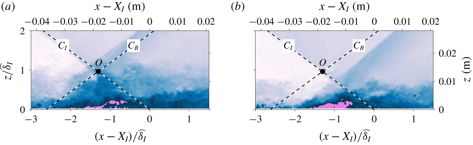
Figure 8(a,b) shows instantaneous streamwise velocity examples where an incident shock impinges on a boundary layer developing over a flat plate, resulting in a reflected shock. As noted in the introduction, one of the striking features of SWBLI is the variation in the shock location due to its oscillation, as illustrated in figure 8 where the reflected shock is located upstream and downstream with respect to the mean shock location denoted by the dashed line.
Instantaneous streamwise velocities when the reflected shock is located (a) upstream and (b) downstream of the mean location,  $C_{R}$, indicated by the dashed line. The colour contours are as in figure 5, and the flow is from left to right.

Joint probability density function of the incident and reflected shock angles,  $\unicode[STIX]{x1D6FD}_{I}$ and
 $\unicode[STIX]{x1D6FD}_{R}$, respectively (a positive
 $\unicode[STIX]{x1D6FD}$ is clockwise in the
 $x$–
 $z$ plane, following the right-hand rule).

4.1 Influences of the oscillating incident shock
In most of the past works examining a shock reflection SWBLI configuration, the incident shock is generated utilising a two-dimensional obstacle placed in the free-stream region (e.g. Dupont et al. Reference Dupont, Haddad and Debieve2006), leading to a relatively fixed incident shock. However, in many practical applications, a series of shock reflections are generated from two opposing walls. Hence, the reflected shock from one side of the wall can impinge on the opposing wall, leading to cases where the incident shocks themselves oscillate. To investigate the influence of oscillating incident shock, the shock generator is fixed to the roof of the wind tunnel in the current work, as illustrated in figure 2. Therefore, the incoming flow to the shock generator is unsteady and contains a wide range of turbulent scales from the boundary layer developing on the roof, resulting in an oscillating incident shock. Furthermore, high-speed schlieren visualisation indicate that the incident shock oscillations are dominated by time scales that are smaller than  $3\,\widehat{\unicode[STIX]{x1D6FF}}_{I}/U_{\infty }$, which corresponded to the smallest resolvable time step from the high-speed visualisation (see § 5 for further details).
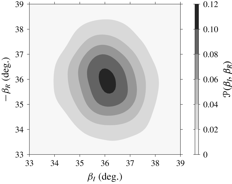
Figure 9 shows the joint probability density function ( j.p.d.f.) of the incident and reflected shock angles. To identify the shock locations, a linear fit is performed through the  $\text{d}\widetilde{U}/\text{d}x$ minima in the free-stream region. The j.p.d.f. shown in figure 9 resembles an upright ellipse, an indication that the two variables are linearly independent with a correlation coefficient approximately equal to 0.08. The independence of
 $\unicode[STIX]{x1D6FD}_{I}$ and
 $\unicode[STIX]{x1D6FD}_{R}$ is contrary to the inviscid theory, where
 $\unicode[STIX]{x1D6FD}_{R}$ is expected to be more perpendicular to the wall when
 $\unicode[STIX]{x1D6FD}_{I}$ increases, suggesting that the instantaneous location of the oscillating incident shock has a minimal influence on the instantaneous reflected shock location, at least in a linear sense (there may be a nonlinear influence as further discussed in § 6.1).
4.2 Influences of the incoming boundary layer
Notably, in figure 8 the incoming boundary layer is thicker when the reflected shock is located upstream of the mean location compared to the case when it is located downstream of the mean location. This suggests that the reflected shock location is influenced by the state of the incoming boundary layer as proposed by Ünalmis & Dolling (Reference Ünalmis and Dolling1998), Beresh et al. (Reference Beresh, Clemens and Dolling2002), Humble et al. (Reference Humble, Elsinga, Scarano and Van Oudheusden2009) and others. To further assess the relation between the state of the incoming boundary layer and the reflected shock location, a subset of the data where the incident shock lies in the range  $\pm 0.25^{\circ }$ of the mean position (corresponding to 15 % of the total dataset), and therefore remains relatively fixed, is used for the subsequent analysis presented in this section.
(a) Two-point correlation coefficient between local boundary layer thickness and reflected shock location. Three choices for the measure of local boundary layer thickness are shown: ○, instantaneous displacement thickness; ▵,  $z_{75}$, i.e.
 $z$ locations where
 $\widetilde{U}=0.75U_{\infty }$; and ♢, upper TNTI envelope. (b) Instantaneous and (c) temporal-averaged streamwise velocity fields, where the colour contours are as in figure 5. The corresponding displacement thickness,
 $z_{75}$ and upper TNTI envelope are indicated by the dashed (– – –), dash-dotted (— ⋅ —) and dotted (
 $\cdots \cdots$) lines.

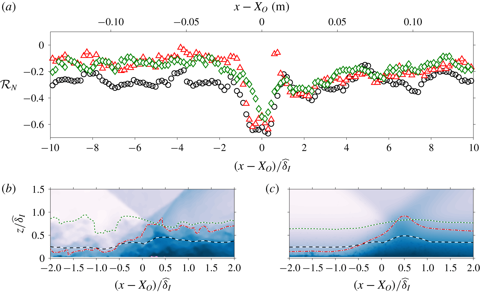
Figure 10(a) shows the correlation coefficient between the instantaneous boundary layer thicknesses and the reflected shock location at various  $x$ locations. Note that, through the interaction region the edge velocity changes as a function of the streamwise location, resulting in difficulties when defining a boundary layer thickness that remains consistent across all
 $x$ locations. In figure 10(a), three choices are considered (their relative locations are demonstrated in figure 10b,c). The circles (○) show the correlation coefficient when the instantaneous displacement thickness,
 $\widetilde{\unicode[STIX]{x1D6FF}}^{\ast }=\int 1-(\unicode[STIX]{x1D70C}_{upstream}\widetilde{U}\,)/(\unicode[STIX]{x1D70C}_{\infty }U_{\infty })\,\text{d}z$, is considered as a measure of the boundary layer thickness. Note that, here,
 $\unicode[STIX]{x1D70C}_{upstream}$ corresponds to the mean density estimated from the mean velocity profile upstream of the shock following Walz’s (Reference Walz1959) relation. The triangles (▵) consider the
 $z$ locations where the velocity is 75 % of the incoming free-stream velocity as a measure of the boundary layer thickness. Lastly, the diamonds (♢) consider the upper envelope of the turbulent/non-turbulent interface (TNTI) as a measure of the boundary layer thickness. Note that, here, the TNTI location is determined from the velocity field based on the local kinetic energy criterion proposed by Reuther & Kähler (Reference Reuther and Kähler2018), where a value close to zero is expected in the free-stream region while a non-zero value occurs within the boundary layer. For full details of the TNTI detection procedure utilised for the current study, the reader is referred to Baidya et al. (Reference Baidya, Scharnowski, Bross and Kähler2019).
All three choices for the boundary layer thickness used in figure 10(a) indicate that the reflected shock location is well correlated ( $|{\mathcal{R}}_{N}|>0.4$) with the instantaneous boundary layer thickness immediately upstream of the SWBLI region. In addition, the instantaneous boundary layer thickness is influenced by the presence of the
 $\unicode[STIX]{x1D6FF}$-scaled structures. Hence, the passage of low-/high-momentum large-scale turbulent features through the interaction region leads to the reflected shock to move upstream/downstream of the mean position, respectively.
Joint probability function of the reflected shock location and TNTI upper envelope,  $z_{TNTI}$. The j.p.d.f. at (a)
 $(x-X_{O})=-2\,\widehat{\unicode[STIX]{x1D6FF}}_{I}$, (b)
 $(x-X_{O})=0$ and (c)
 $(x-X_{O})=2\,\widehat{\unicode[STIX]{x1D6FF}}_{I}$ is shown.

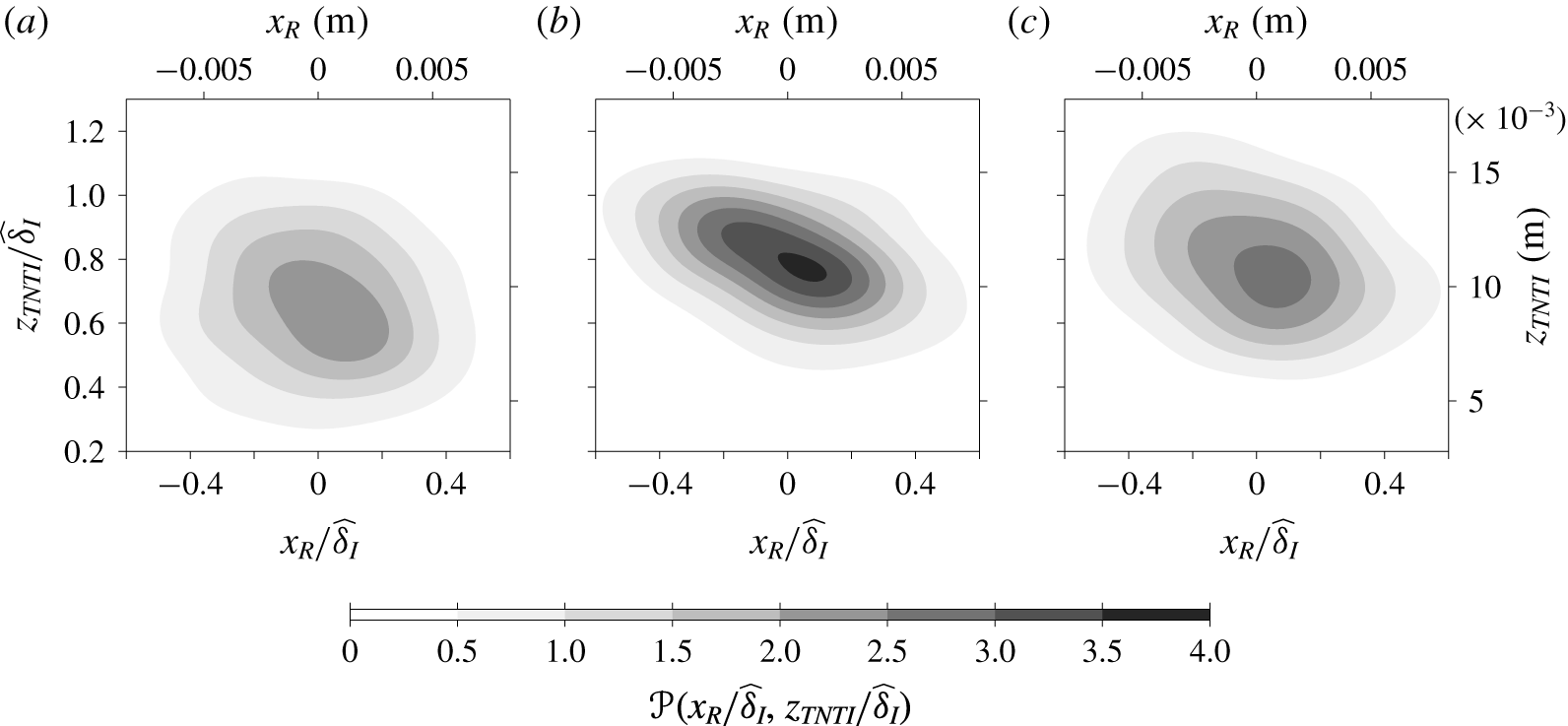
To further quantify how the two-point correlation coefficient,  ${\mathcal{R}}_{N}$, changes as a function of the streamwise location, figure 11(a–c) shows the j.p.d.f. of the reflected shock location and TNTI upper envelope at
 $(x-X_{O})/\,\widehat{\unicode[STIX]{x1D6FF}}_{I}=-2$, 0 and 2, respectively. Here,
 $X_{O}$ corresponds to the
 $x$ location where the mean locations of the incident and reflected shock intersect (i.e. point
 $O$ in figure 8). In the vicinity of
 $x=X_{O}$, the TNTI upper envelope correlates most strongly with the reflected shock (
 ${\mathcal{R}}_{N}\approx -0.5$), leading to a j.p.d.f. resembling an inclined elongated ellipse. Upstream of the SWBLI region, the degree of correlation drops rapidly and
 ${\mathcal{R}}_{N}\approx -0.1$ is reached at
 $(x-X_{O})/\,\widehat{\unicode[STIX]{x1D6FF}}_{I}=-2$, and consequently, the j.p.d.f. is circular in shape. In contrast, the drop in correlation downstream of the shock is much more gradual and
 ${\mathcal{R}}_{N}\approx -0.3$ is reached at
 $(x-X_{O})/\,\widehat{\unicode[STIX]{x1D6FF}}_{I}=2$. Hence, the j.p.d.f. at
 $(x-X_{O})/\,\widehat{\unicode[STIX]{x1D6FF}}_{I}=2$ is more elliptical than at
 $(x-X_{O})/\,\widehat{\unicode[STIX]{x1D6FF}}_{I}=-2$. The gradual approach to
 ${\mathcal{R}}_{N}=0$ suggests that the instantaneous velocity profiles several boundary layer thicknesses downstream of SWBLI are modified by the presence of the shock, which is consistent with the long recovery observed for the mean and variance statistics in § 3.
Conditional statistics based on the  $\widetilde{C}_{R}$ shock foot (streamwise) location. The left (a,c) and right (b,d) columns show the ensemble-averaged streamwise velocity and Reynolds shear stress, respectively. The top row (a,b) corresponds to instances when the shock foot is upstream from the mean value, while the bottom row (c,d) corresponds to the downstream instances. The colour and line contour shown in (a) and (c) are at levels 0.2 to 0.8 in steps of 0.2, where the dotted lines indicate the contours of ensemble-averaged
 $\widetilde{U}$ over all instances when the location of
 $\widetilde{C}_{I}$ is fixed. The dashed lines in (b) and (d) correspond to
 $-\langle uw\rangle /U_{\infty }^{2}=-0.2\times 10^{-3}$ contours, while the dotted lines are as in (a) and (c) for the 0.2
 $\langle \widetilde{U}\rangle /U_{\infty }$ level. The grey lines denote the mean incident (
 $C_{I}$) and reflected (
 $C_{R}$) shock locations.

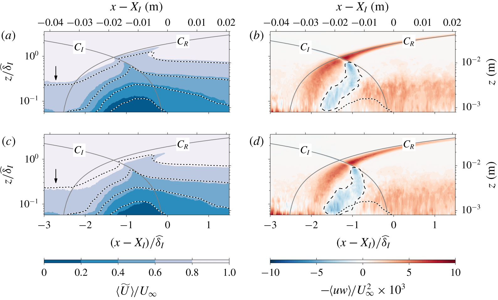
Figure 12 shows the conditional statistic results based on the streamwise location of the reflected shock foot. Figure 12(a,b) shows the conditional statistics for the third of cases when the shock foot is at the most upstream location. Conversely, figure 12(c,d) corresponds to the third of cases when the shock foot is at the most downstream location. The colour contours shown in figure 12(a,c) corresponds to the ensemble-averaged streamwise velocity,  $\langle \widetilde{U}\rangle$, while the dotted lines show iso-contours of the ensemble average from the entire dataset when the incident shock location
 $\widetilde{C}_{I}$ is fixed. Both the colour and line contours are at levels 0.2 to 0.8 in steps of 0.2. Due to issues with obtaining accurate velocity measurements in the vicinity to the wall from the large FOV configuration utilised in the current study, the conditional statistics shown in figure are only reliable starting from 0.8 mm away from the wall and are unfortunately unable to capture the separation region (however, we are able to observe instances with separation – see figure 8). Nevertheless, other studies where the separation bubble is resolved show that the decrease/increase in the zero-velocity isocontour corresponding to the separation bubble size is accompanied by the decrease/increase of other velocity isocontour levels (Piponniau et al. Reference Piponniau, Dussauge, Debieve and Dupont2009; Grilli et al. Reference Grilli, Schmid, Hickel and Adams2012; Priebe & Martín Reference Priebe and Martín2012). Hence, the higher velocity isocontour level is typically used as a surrogate for the behaviour of the separation bubble when the zero-velocity isocontour is not experimentally accessible (Ganapathisubramani et al. Reference Ganapathisubramani, Clemens and Dolling2007; Ganapathisubramani, Clemens & Dolling Reference Ganapathisubramani, Clemens and Dolling2009). From comparisons of the 0.2 level, it is evident that the region where
 $\langle \widetilde{U}\rangle <0.2U_{\infty }$ is smaller in (c) compared to (a). Furthermore, comparison of
 $\langle \widetilde{U}\rangle =0.8U_{\infty }$ at the
 $x$ locations indicated by arrows shows that the incoming boundary layer is thinner in (c) compared to (a). Since the
 $\unicode[STIX]{x1D6FF}$-scaled structures play a critical role in determining the instantaneous boundary layer thickness, the present results support the direct link between the passage of very-large-scale structures through the interaction region and the expansion and contraction of the separation bubble proposed by Ganapathisubramani et al. (Reference Ganapathisubramani, Clemens and Dolling2007, Reference Ganapathisubramani, Clemens and Dolling2009). A similar correlation between the passage of very-large-scale structures and the expansion/contraction of the separation bubble (for this particular case the separation bubble was well resolved using a highly magnified FOV PIV, unlike for the current experiment) has also been observed in adverse-pressure-gradient turbulent boundary layer flows (Bross, Fuchs & Kähler Reference Bross, Fuchs and Kähler2019a). Furthermore, a region of strongly negative Reynolds shear stress is observed to move downstream with the shock foot (see the dashed lines relative to dotted lines in figure 12b,d), which notably coincides with the shrinking of
 $\langle \widetilde{U}\rangle =0.2U_{\infty }$ contour observed at
 $(x-X_{I})/\,\widehat{\unicode[STIX]{x1D6FF}}_{I}\approx -1.5$. Thus, the data suggest that the expansion and contraction of the separation bubble is strongly influenced by the ejection and sweep mechanisms associated with the low- and high-momentum fluid that dominates the Reynolds shear stress contributions.
5 Analysis of wall pressure signals
In the past, experimental investigations of SWBLI were mostly based solely on wall pressure measurements. One of the key findings from these works is that the oscillation of the shock foot leads to pressure fluctuations that are dominated by time scales that are orders of magnitude slower than the time scales associated with the very-large-scale motions residing in the boundary layer. This large separation of the scales is one of the leading arguments presented by the researchers who argue that the influence of the incoming boundary layer is not the dominant mechanism responsible for the reflected shock oscillations (e.g. Piponniau et al. Reference Piponniau, Dussauge, Debieve and Dupont2009). However, the origin of the low-frequency oscillation has not been fully resolved, which we aim to redress in the current work, through examination of a dataset where a plane of velocity and wall pressure are simultaneously captured.
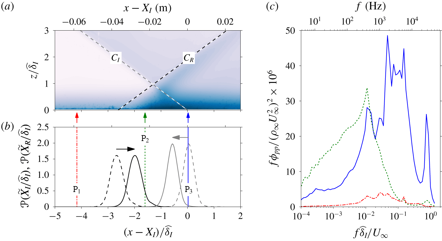
(a) Mean streamwise velocity, where the colour contours are as in figure 5. (b) Probability density function of the incident (grey lines) and reflected (black lines) shock foot locations, where the dashed lines show the shock location based on a linear fit in the free-stream region. The solid lines denote the shifted p.d.f. (as indicated by the horizontal arrows) accounting for the deviation from the linear fit due to presence of a boundary layer, based on the mean field. (c) Pre-multiplied pressure spectra. The location of the pressure transducer is indicated by the arrows in (a) coloured according to the lines.

Figure 13(a) shows the location of three fast-response pressure transducer relative to the mean shock location. In addition, (b) shows the probability density function (p.d.f.) of the incident and reflected shock foot locations, where the dashed lines denote the p.d.f. based on a linear fit to the  $\text{d}\widetilde{U}/\text{d}x$ minima in the free-stream region extrapolated to the wall. Meanwhile, the solid lines correspond to the p.d.f. accounting for the deviations from the straight line due to the presence of the boundary layer, based on the
 $U$ field. From figure 13(b), it is evident that the oscillation of the shock foot does not extend to
 $\mathtt{P}_{1}$ (location shown in dash-dotted line), while the pressure signals from
 $\mathtt{P}_{2}$ and
 $\mathtt{P}_{3}$ (locations shown by dotted and solid lines) contain fluctuations due to movement of the reflected and incident shock feet relative to the sensors. Hence, the pressure fluctuations recorded by
 $\mathtt{P}_{2}$ and
 $\mathtt{P}_{3}$ are significantly more energetic compared to
 $\mathtt{P}_{1}$ as evident from the pressure spectra,
 $\unicode[STIX]{x1D719}_{pp}$, shown in figure 13(c) where
 $\int _{0}^{\infty }f\unicode[STIX]{x1D719}_{pp}\,\text{d}f=\overline{p^{2}}$. Furthermore, the wall pressure fluctuation captured by the sensor
 $\mathtt{P}_{2}$ has a dominant frequency at
 $f\,\widehat{\unicode[STIX]{x1D6FF}}_{I}/U_{\infty }\sim 10^{-2}$ associated with the oscillation of the reflected shock foot, which is consistent with the observations by Grilli et al. (Reference Grilli, Schmid, Hickel and Adams2012), Priebe & Martín (Reference Priebe and Martín2012) and others. Touber & Sandham (Reference Touber and Sandham2009) find that the dominant wall pressure mode also agrees with the linear stability analysis conducted on the mean LES fields, where the unstable global mode has a time scale that is
 $O(10^{2}\,\widehat{\unicode[STIX]{x1D6FF}}/U_{\infty })$. Furthermore, Pirozzoli et al. (Reference Pirozzoli, Larsson, Nichols, Bernardini, Morgan and Lele2010) observe that the modes containing turbulent structures from the dynamic mode decomposition analysis occur at a much higher frequency (by two orders of magnitude) compared to the dominant mode of the separation bubble unsteadiness. This has led some researchers to argue that the unstable global mode is the main mechanism that drives the expansion–contraction cycle of the separation bubble and hence the shock oscillation (Touber & Sandham Reference Touber and Sandham2009; Priebe & Martín Reference Priebe and Martín2012). However, the reflected shock oscillations are clearly influenced by the incoming boundary layer for the current dataset, as discussed in § 4.2, and since the low-frequency pressure oscillations are found to correlate well with the shock oscillations (see figure 14), the current results suggest that these two phenomena are related even though there is a two orders of magnitude difference in the dominant time scales.
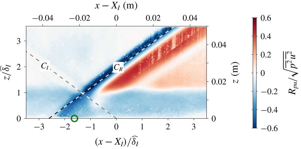
Figure 14 shows the pressure–velocity correlation at a zero time offset between the velocity and pressure signals from the planar PIV and sensor  $\mathtt{P}_{2}$, respectively. The velocities in the free-stream region, that are in the vicinity of the mean reflected shock location, are well correlated with the pressure signal. It should be noted that the
 $u$ fluctuations in the free stream are an artefact from the use of Reynolds decomposition and the oscillation of the shock front. That is, when a shock front travels upstream, a low-momentum region relative to the mean value is formed immediately downstream of the shock. Conversely, when a shock front moves downstream, a high-momentum region is present immediately upstream of the shock. Thus, figure 14 indicates that the oscillation of the reflected shock is well correlated with the pressure fluctuations registered by
 $\mathtt{P}_{2}$.
Pressure–velocity two-point correlation coefficient. Here, the pressure signal from sensor  $\mathtt{P}_{2}$, located at the circle symbol (○), is the reference.

Unlike the sensor  $\mathtt{P}_{2}$, figure 13(c) indicates that the pressure spectrum from
 $\mathtt{P}_{3}$ has two distinct peaks at
 $f\,\widehat{\unicode[STIX]{x1D6FF}}_{I}/U_{\infty }\sim 10^{-2}$ and
 $10^{0}$. In addition, a dominant broadband mode with a near-uniform energetic content (a plateau in the pre-multiplied spectra) is observed at
 $5\times 10^{-2}\lesssim f\,\widehat{\unicode[STIX]{x1D6FF}}_{I}/U_{\infty }\lesssim 2\times 10^{-1}$. The pressure–velocity correlation for the band-passed pressure signal to extract these dominant modes indicates that while the mode at
 $f\,\widehat{\unicode[STIX]{x1D6FF}}_{I}/U_{\infty }\sim 10^{-2}$ correlates with both the incident and reflected shock oscillations (a correlation coefficient of approximately 0.25), non-significant correlations are observed for the broadband and
 $f\,\widehat{\unicode[STIX]{x1D6FF}}_{I}/U_{\infty }\sim 10^{0}$ modes. In contrast, the wall pressure signal captured by sensor
 $\mathtt{P}_{2}$ exhibits strong correlation only with the reflected shock oscillation (see figure 14 where
 $R_{pu}\approx 0$ in the vicinity of
 $C_{I}$), and therefore the unsteady reflected shock foot behaviour is best captured by sensor
 $\mathtt{P}_{2}$ and the subsequent analysis presented will be based on the wall pressure signal from this sensor.
In addition to examining how the correlation  $R_{pu}$ varies in space, one can also look at how the correlation decays as the time offset,
 $\unicode[STIX]{x0394}t$, between signals
 $p(t)$ and
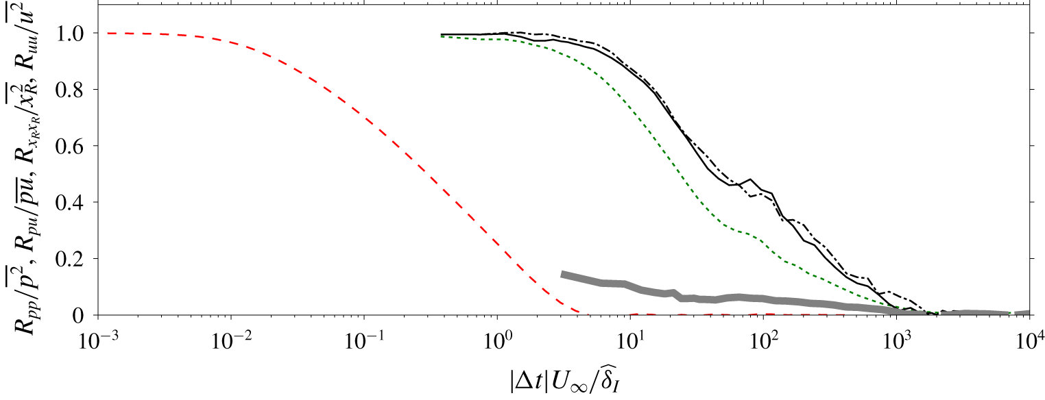
 $u(t+\unicode[STIX]{x0394}t)$ is increased. Figure 15 shows
 $R_{pu}$ as a function of
 $\unicode[STIX]{x0394}t$, where the negative and positive offsets are indicated using the dash-dotted and solid lines, respectively. Here, the
 $u$ signal is taken in the free-stream region corresponding to the location where the strongest correlation between the wall pressure signal and the velocity fields is observed in figure 14. More specifically, the correlated
 $u$ velocity corresponds to an averaged velocity along a line approximately
 $0.05\,\widehat{\unicode[STIX]{x1D6FF}}$ upstream of the mean reflected shock position in the region
 $z/\widehat{\unicode[STIX]{x1D6FF}}_{I}\geqslant 1.4$. Also shown are autocorrelations of the wall pressure signal from sensor
 $\mathtt{P}_{2}$ (dotted line), the
 $u$ velocity in the logarithmic region of a canonical incompressible boundary layer (dashed line) and the reflected shock location based on schlieren images (thick solid line) for comparison purposes. Note that, here, the sampling frequency for the schlieren images is not sufficiently high to capture the small-scale energetic contributions, leading to an incomplete
 $R_{x_{R}x_{R}}$. Similarly, the incident shock oscillation is also not fully captured by the high-speed schlieren visualisation (the normalised temporal correlation of the incident shock location is found to be very similar to that of the reflected shock location and is therefore not shown here for brevity). Furthermore, although
 $R_{uu}$ is not from the current configuration, based on Morkovin’s (Reference Morkovin and Favre1962) hypothesis the large-scale energetic contents in compressible and incompressible boundary layers are expected to reside at similar multiples of the boundary layer thickness (Pirozzoli & Bernardini Reference Pirozzoli and Bernardini2011).
Comparisons of energetic scales in the pressure ( $p$) and reflected shock location (
 $x_{R}$) fluctuations. The dotted line (
 $\cdots \cdots$) corresponds to the temporal correlation of the wall pressure signal, while a pressure–velocity correlation with a velocity in the free-stream region is shown by dash-dotted (— ⋅ —) and solid lines (——) for the negative and positive time offsets, respectively. The temporal correlation of
 $x_{R}$, obtained from schlieren images, is shown as a thick grey line. In addition, the streamwise velocity correlation,
 $R_{uu}$, in the logarithmic region of a canonical, incompressible turbulent boundary layer from Baidya et al. (Reference Baidya, Philip, Hutchins, Monty and Marusic2017) is indicated with the dashed line (– – –).

The time offsets where the normalised temporal correlations, shown in figure 15, deviate from unity and zero correspond to the energetic range of scales. Thus, as reported by past researchers, the pressure fluctuations are dominated by time scales that are orders of magnitude slower than the time scales associated with the very-large-scale structures that reside in the logarithmic region. Since  $R_{x_{R}x_{R}}\ll \overline{x_{R}^{2}}$ at
 $(\unicode[STIX]{x0394}tU_{\infty })/\widehat{\unicode[STIX]{x1D6FF}}_{I}\approx 3$, while
 $R_{pp}\approx \overline{p^{2}}$, the reflected shock positions in the free stream,
 $x_{R}$, are dominated by time scales smaller than
 $O(\,\widehat{\unicode[STIX]{x1D6FF}}_{I}/U_{\infty })$, in contrast to the pressure fluctuations. Therefore, based on the strong correlation observed between the large-scale structure entering the SWBLI region and
 $x_{R}$ (see § 4), we postulate that the
 $u$ fluctuation in the incoming boundary layer and the
 $x_{R}$ fluctuations are dominated by time scales that are similar in order of magnitude. Moreover, a strong correlation between the wall pressure and the velocity in the vicinity of the shock (see figure 14) and the fact that the correlation is dominated by time scales that are
 $(\unicode[STIX]{x0394}tU_{\infty })/\widehat{\unicode[STIX]{x1D6FF}}_{I}\gtrsim O(10)$ (see figure 15) suggest that the movement of the reflected shock in the free stream and the movement of its foot at the wall are only linear for the low-frequency contents. Therefore, the scales excited through the SWBLI region by the incoming boundary layer perturbations seem to exhibit a wall-normal dependency. In particular, higher-frequency contents beyond the unstable global mode associated with the interaction region seem to be dampened and only the low-frequency contents transferred to the shock foot, leading to a dominant mode in the wall pressure signal that is two orders of magnitude smaller than the dominant energetic mode observed for the incoming boundary layer. Evidence exists which indicate different levels of influence from the upstream and downstream effects on the separation bubble unsteadiness as a function of its frequency content. For example, Vanstone & Clemens (Reference Vanstone and Clemens2019) show based on band-pass filtered high-speed PIV data that, while the low (
 $f\,\widehat{\unicode[STIX]{x1D6FF}}_{I}/U_{\infty }<10^{-2}$) and medium (
 $10^{-2}<f\,\widehat{\unicode[STIX]{x1D6FF}}_{I}/U_{\infty }<10^{-1}$) frequency contents exhibit strong correlation with the low- and high-momentum events in the upstream boundary layer, the high (
 $f\,\widehat{\unicode[STIX]{x1D6FF}}_{I}/U_{\infty }>10^{-1}$) frequency contents appear to be primarily driven by shear layer flapping from the downstream region. Hence for cases when the separation is stronger, the perturbation at time scales corresponding to the unstable global mode may be dominated by sources other than the perturbations from the incoming boundary layer, leading to reduced influence of the upstream boundary layer for these cases, as reported by Piponniau et al. (Reference Piponniau, Dussauge, Debieve and Dupont2009), Clemens & Narayanaswamy (Reference Clemens and Narayanaswamy2014) and others.
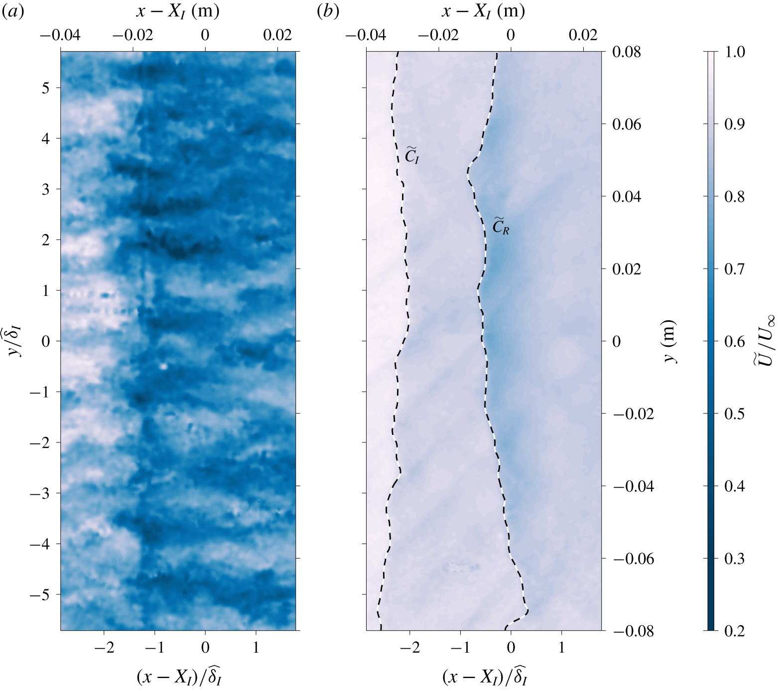
Instantaneous wall-parallel plane of the streamwise velocity. The flow is from left to right and (a) and (b) correspond to  $z$ locations in the outer region of the boundary layer (
 $z/\,\widehat{\unicode[STIX]{x1D6FF}}_{I}\approx 0.4$) and the free-stream region (
 $z/\,\widehat{\unicode[STIX]{x1D6FF}}_{I}\approx 1.7$), respectively.

6 Spanwise characteristics of the shock and its interactions
Figure 16 shows instantaneous examples of wall-parallel velocity fields in the outer region of the boundary layer at  $z/\,\widehat{\unicode[STIX]{x1D6FF}}_{I}\approx 0.4$ (a) and in the free-stream region at
 $z/\,\widehat{\unicode[STIX]{x1D6FF}}_{I}\approx 1.7$ (b). The field shown in figure 16(a) exhibits distinct low- and high-momentum streaks with a spanwise spacing of
 $O(\unicode[STIX]{x1D6FF})$, which is consistence with a presence of counter-rotating Görtler-like vortices observed by Pasquariello, Hickel & Adams (Reference Pasquariello, Hickel and Adams2017) downstream of the SWBLI region. However, the curvature criterion based on a streamline from the mean field, given by Smits & Dussauge (Reference Smits and Dussauge2006) and Pasquariello et al. (Reference Pasquariello, Hickel and Adams2017), is not met in the recovery region (
 $x$ location downstream of where the minimum
 $U$ occurs within the interaction region) for the current case and therefore these features may also be related to the low- and high-momentum very-large-scale structures entering the interaction region (Humble et al. Reference Humble, Elsinga, Scarano and Van Oudheusden2009), which are also observed to have a spanwise spacing of
 $O(\unicode[STIX]{x1D6FF})$. The presence of the shock leads to a sharp change in
 $\widetilde{U}$, and in the free-stream region the location of the shock can be identified based on
 $\text{d}\widetilde{U}/\text{d}x$ minima, as illustrated in figure 16(b). However, within the boundary layer, the change in
 $\widetilde{U}$ due to the shock is more difficult to identify as its magnitude is of the order of or smaller than the turbulent
 $u$ fluctuations (see figure 16a), even though there is a clear influence from the shock on the mean field at this wall height. From figure 16(b), it is evident that the shock fronts undulate as a function of spanwise location, leading to a rippling pattern on a wall-parallel plane. Besides the location of the incident and reflected shocks, elevated values for the
 $\text{d}\widetilde{U}/\text{d}x$ magnitude appear in figure 16(b) as diagonal lines. These diagonal lines correspond to shocks formed due to the presence of suction holes (used to reduce the influence of the boundary layer developing over the side walls during subsonic experiments) on the test section side walls.
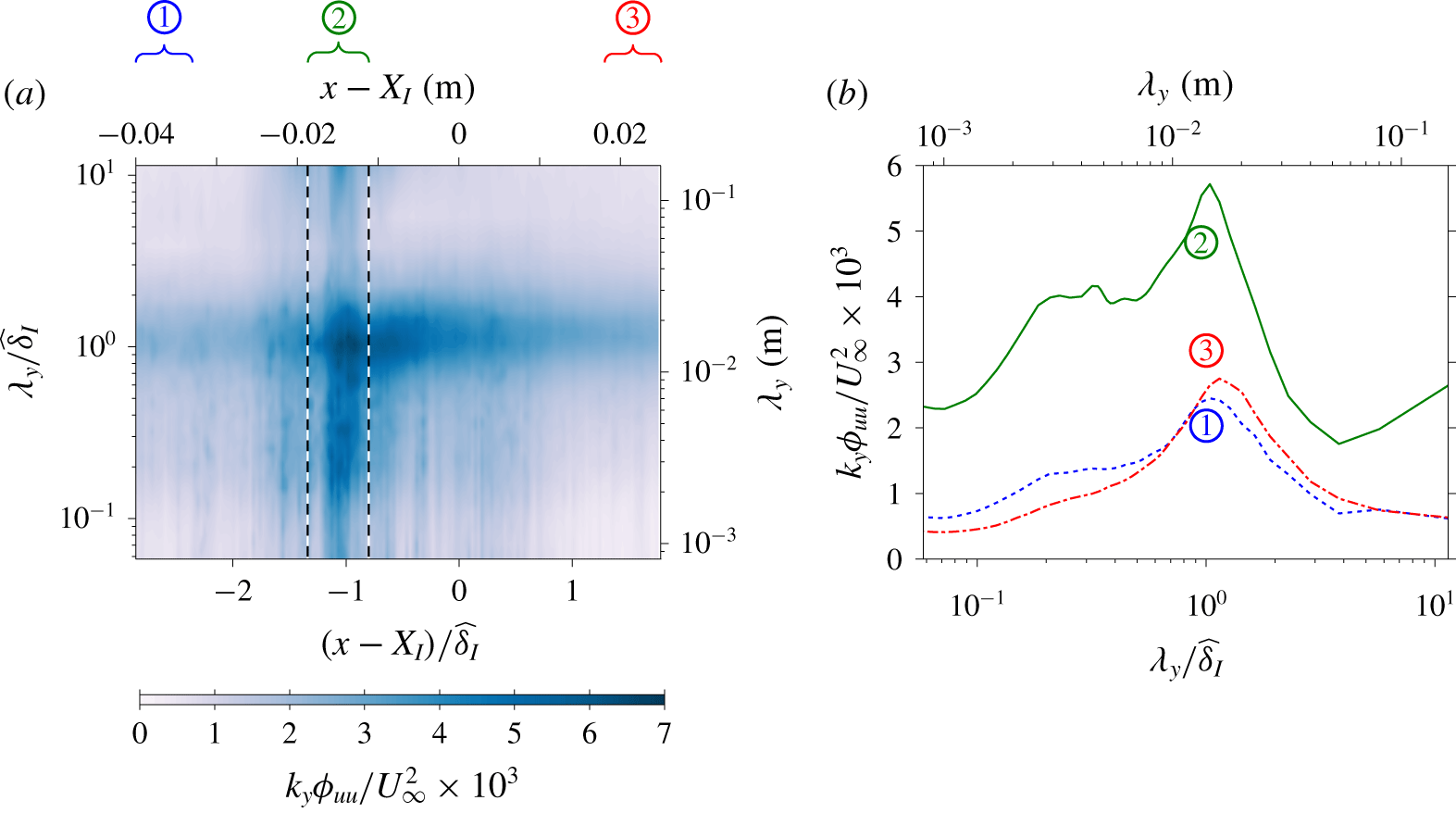
Pre-multiplied spanwise spectra of the streamwise velocity at  $z/\,\widehat{\unicode[STIX]{x1D6FF}}_{I}\approx 0.4$. (a) Spanwise spectra as a function of
 $x$, where the vertical dashed lines denote the location of the incident and reflected shocks based on the mean
 $U$ field. (b) Spatially averaged one-dimensional spectra over the streamwise domains
 $\unicode[STIX]{x2460}$,
 $\unicode[STIX]{x2461}$ and
 $\unicode[STIX]{x2462}$ as indicated in (a).

Figure 17(a) shows the pre-multiplied spanwise  $u$-spectra,
 $k_{y}\unicode[STIX]{x1D719}_{uu}$, as a function of streamwise displacement relative to the shock locations. Here,
 $k_{y}$ and
 $\unicode[STIX]{x1D706}_{y}$ correspond to the spanwise wavenumber and wavelength, respectively (i.e.
 $\unicode[STIX]{x1D706}_{y}=2\unicode[STIX]{x03C0}/k_{y}$). Upstream of the shock, in region
 $\unicode[STIX]{x2460}$, the
 $u$-spectrum is close to
 $x$-invariant as the growth in the boundary layer with respect to
 $x$ is minimal. Within the interaction region, region
 $\unicode[STIX]{x2461}$, strong
 $u$ fluctuations that are energetic over a wide range of scales are introduced by the shocks. Downstream of the interaction region, the flow recovers towards a canonical state and the excessive
 $u$ fluctuations are dissipated and a near
 $x$-invariant
 $u$-spectrum is observed at the most downstream location within the FOV, indicated as region
 $\unicode[STIX]{x2462}$. Figure 17(b) shows the streamwise-averaged spectra over regions
 $\unicode[STIX]{x2460}$–
 $\unicode[STIX]{x2462}$ as a function of
 $\unicode[STIX]{x1D706}_{y}$. Notably, the dominant spanwise mode remains at
 $O(\,\widehat{\unicode[STIX]{x1D6FF}}_{I})$ for regions
 $\unicode[STIX]{x2460}$–
 $\unicode[STIX]{x2462}$, which coincides with the dominant spanwise length scale of large-scale and very-large-scale motions present in wall-bounded flows (Kim & Adrian Reference Kim and Adrian1999). Moreover, the spanwise mode of
 $O(10\,\widehat{\unicode[STIX]{x1D6FF}}_{I})$ seems to be excited in region
 $\unicode[STIX]{x2461}$, in contrast to decay of the energetic content for modes
 $\unicode[STIX]{x1D706}_{y}>\widehat{\unicode[STIX]{x1D6FF}}_{I}$ observed for regions
 $\unicode[STIX]{x2460}$ and
 $\unicode[STIX]{x2462}$. However, the physical mechanisms that would lead to the creation of structures with such a wide correlation are not clear and these modes could be an artefact associated with the wind tunnel and field of view employed rather than being a feature due to SWBLI.
6.1 Behaviour of spanwise scales as a function of the streamwise location
The presence of the shock alters the behaviour of the spanwise scales, as evident from figure 17. Here, how these spanwise scales are altered as a function of the streamwise location from the shock front is further investigated by means of cross-spectrum between  $u(x_{ref})$ and
 $u(x_{ref}+\unicode[STIX]{x0394}x)$. The cross-spectrum
 $\unicode[STIX]{x1D719}_{u_{ref}u_{\unicode[STIX]{x0394}x}}$ is defined as
 $$\begin{eqnarray}\unicode[STIX]{x1D719}_{u_{ref}u_{\unicode[STIX]{x0394}x}}(x_{ref},\unicode[STIX]{x0394}x;\unicode[STIX]{x1D706}_{y})={\mathcal{F}}_{y}(\langle u(x_{ref},y_{ref})u(x_{ref}+\unicode[STIX]{x0394}x,y_{ref}+\unicode[STIX]{x0394}y)\rangle ),\end{eqnarray}$$
where  ${\mathcal{F}}_{y}$ denotes the Fourier transform in the spanwise direction, while
 $\unicode[STIX]{x0394}x$ and
 $\unicode[STIX]{x0394}y$ are streamwise and spanwise displacements relative to the reference point
 $(x_{ref},y_{ref})$.
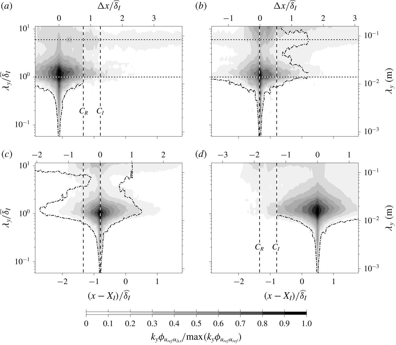
The  $\unicode[STIX]{x1D719}_{u_{ref}u_{\unicode[STIX]{x0394}x}}$ cross-spectrogram at (a)
 $(x_{ref}-X_{I})/\,\widehat{\unicode[STIX]{x1D6FF}}_{I}=-2$, (b)
 $(x_{ref}-X_{I})/\,\widehat{\unicode[STIX]{x1D6FF}}_{I}\approx -1.25$, (c)
 $(x_{ref}-X_{I})/\,\widehat{\unicode[STIX]{x1D6FF}}_{I}\approx -0.75$ and (d)
 $(x_{ref}-X_{I})/\,\widehat{\unicode[STIX]{x1D6FF}}_{I}=0.5$. The colour contours are at levels 0.1 to 0.9 in steps of 0.1, while the line contours correspond to
 $k_{y}\unicode[STIX]{x1D719}_{u_{ref}u_{\unicode[STIX]{x0394}x}}(x_{ref},-\unicode[STIX]{x0394}x;\unicode[STIX]{x1D706}_{y})/\max (k_{y}\unicode[STIX]{x1D719}_{u_{ref}u_{ref}})=0.1$ (i.e. the colour contour 0.1 level reflected about the
 $\unicode[STIX]{x0394}x=0$ axis). The horizontal dotted lines correspond to
 $\unicode[STIX]{x1D706}_{y}/\,\widehat{\unicode[STIX]{x1D6FF}}_{I}=1$ and
 $\unicode[STIX]{x1D706}_{y}/\,\widehat{\unicode[STIX]{x1D6FF}}_{I}=6$, while the vertical dashed lines denote the mean incident and reflected shock locations.

Figure 18(a–d) shows  $\unicode[STIX]{x1D719}_{u_{ref}u_{\unicode[STIX]{x0394}x}}$ cross-spectrogram normalised by
 $\max (k_{y}\unicode[STIX]{x1D719}_{u_{ref}u_{ref}})$ when the reference
 $x$ location is upstream, in the vicinity and downstream of the SWBLI region. In addition to colour contours at levels 0.1 to 0.9 in steps of 0.1, the line contours show the lowest colour contour level reflected about the
 $\unicode[STIX]{x0394}x=0$ axis. Thus, by comparing the 0.1 colour contour and the dash-dotted line, the upstream and downstream
 $\unicode[STIX]{x1D719}_{u_{ref}u_{\unicode[STIX]{x0394}x}}$ behaviour can be compared. For example, at
 $(x_{ref}-X_{I})/\,\widehat{\unicode[STIX]{x1D6FF}}_{I}=-2$ the cross-spectrogram is nearly symmetric about the reference point for spanwise scales
 $\unicode[STIX]{x1D706}_{y}/\,\widehat{\unicode[STIX]{x1D6FF}}_{I}<0.6$, since 0.1 level colour and line contours exhibit a good collapse. Also note that for an unmodified boundary layer the cross-spectrogram is near symmetric for all scales as the change with respect to
 $x$ is minimal.
At spanwise wavelengths larger than  $\widehat{\unicode[STIX]{x1D6FF}}_{I}$, figure 18(a–d) suggests that the
 $u$ fluctuations retain correlation even after being modified by the shock. At
 $(x_{ref}-X_{I})/\,\widehat{\unicode[STIX]{x1D6FF}}_{I}\approx -1.25$, two persistent modes,
 $\unicode[STIX]{x1D706}_{y}/\,\widehat{\unicode[STIX]{x1D6FF}}_{I}\approx 1$ and
 $\unicode[STIX]{x1D706}_{y}/\,\widehat{\unicode[STIX]{x1D6FF}}_{I}\approx 6$, are evident and they remain correlated over longer streamwise distances compared to other spanwise wavelengths. Furthermore, the persistent mode at
 $\unicode[STIX]{x1D706}_{y}/\,\widehat{\unicode[STIX]{x1D6FF}}_{I}\approx 6$ shifts towards a wider spanwise length scales downstream of the interaction region. Since the boundary layer thickens downstream of the interaction region, the widening of the spanwise length scales may be an indication that these highly persistent modes scale with the local boundary layer thickness. However, it should be noted that the very wide persistent mode is close to the full FOV of the current experiment and therefore the cross-spectra can only be resolved at limited wavelengths at these scales, and experiments with a much wider FOV are necessary to confirm these findings. The dual persistent modes are again evident at
 $(x_{ref}-X_{I})/\,\widehat{\unicode[STIX]{x1D6FF}}_{I}\approx -0.75$, and the correlations are generally retained longer downstream of
 $x_{ref}$ compared to upstream where the
 $u$ fluctuations are modified by the shock. Finally, at
 $(x_{ref}-X_{I})/\,\widehat{\unicode[STIX]{x1D6FF}}_{I}=0.5$, the small scales exhibit symmetry in the
 $x$ direction about the reference point, suggesting that these scales depend only on the local conditions, while the larger spanwise scales still retain influence from modifications due to shock and are yet to recover to a canonical state. Note that to verify that the highly persistent modes observed are not an artefact of the wind tunnel, where spanwise variations that are
 $O(\widehat{\unicode[STIX]{x1D6FF}})$ can be generated within the boundary layer due to slight wind tunnel imperfections (Townsend Reference Townsend1976), further SWBLI experiments with a different incoming boundary layer thickness are necessary.
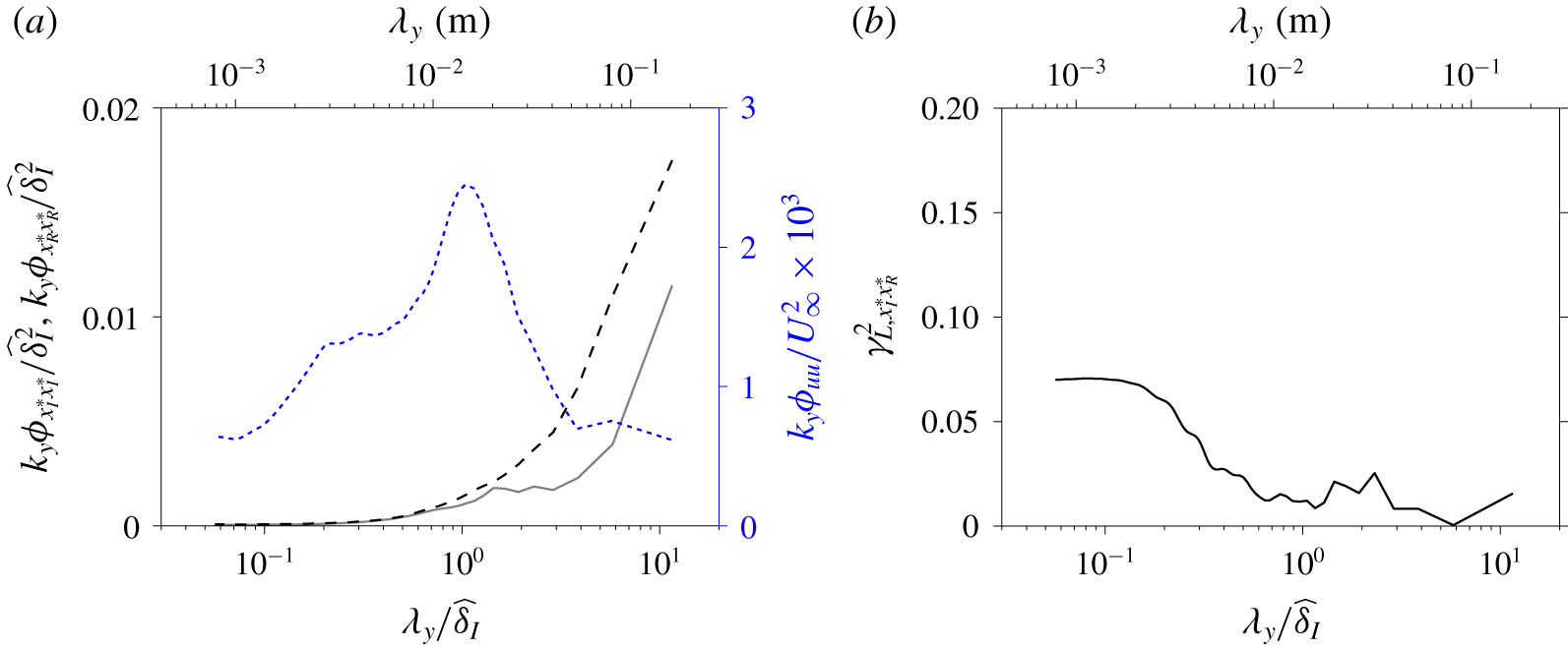
(a) Pre-multiplied spanwise spectra of the streamwise shock location captured on the plane  $z/\,\widehat{\unicode[STIX]{x1D6FF}}_{I}\approx 1.7$. The solid (——) and dashed (– – –) lines correspond to the incident and reflected shock locations,
 $x_{I}^{\ast }$ and
 $x_{R}^{\ast }$, respectively. Also shown in (a) as a dotted (
 $\cdots \cdots$) line is the pre-multiplied
 $u$-spectra for the incoming boundary layer at
 $z/\,\widehat{\unicode[STIX]{x1D6FF}}_{I}\approx 0.4$ (i.e.
 $u$-spectra corresponding to region
 $\unicode[STIX]{x2460}$ from figure 17b). (b) Linear coherence spectra of incident and reflected shock locations.

Figure 19(a) shows the pre-multiplied spanwise spectra of the incident (——) and reflected (– – –) shock locations. It should be noted that the incident and reflected shock fluctuations,  $x_{I}^{\ast }$ and
 $x_{R}^{\ast }$, respectively, are based on wall-parallel PIV conducted at
 $z/\,\widehat{\unicode[STIX]{x1D6FF}}_{I}\approx 1.7$. Also shown overlaid is the
 $u$-spectra of the incoming boundary layer in the outer region of the boundary layer (
 $\cdots \cdots$). From the figure, it is evident that the spanwise scales of the reflected shock location become increasingly energetic at wider spanwise length scales when
 $\unicode[STIX]{x1D706}_{y}/\,\widehat{\unicode[STIX]{x1D6FF}}_{I}\gtrsim 4$, while the energetic
 $u$ motion of the incoming boundary layer remains approximately constant at these length scales. Hence, the increase in the energetic content of
 $x_{R}^{\ast }$ at these spanwise scales is unlikely to originate from the incoming boundary layer. In contrast to the
 $u$-spectra, an increased energetic contribution at a wider spanwise scale, similar to that observed for the reflected shock location, is also observed for the incident shock location. Thus, the data suggest that the increasing energetic contribution at a very wide spanwise scale (
 $\unicode[STIX]{x1D706}_{y}/\,\widehat{\unicode[STIX]{x1D6FF}}_{I}>4$) for the reflected shock is due to influence of increasing energetic content for the incident shock at these scales. Figure 19(b) shows the linear coherence spectra of the incident and reflected shock oscillations. Here, the linear coherence spectra,
 $\unicode[STIX]{x1D6FE}_{L,x_{I}^{\ast }x_{R}^{\ast }}^{2}$ is defined as
 $$\begin{eqnarray}\unicode[STIX]{x1D6FE}_{L,x_{I}^{\ast }x_{R}^{\ast }}^{2}(\unicode[STIX]{x1D706}_{y})=\frac{|\unicode[STIX]{x1D719}_{x_{I}^{\ast }x_{R}^{\ast }}(\unicode[STIX]{x1D706}_{y})|^{2}}{\unicode[STIX]{x1D719}_{x_{I}^{\ast }x_{I}^{\ast }}(\unicode[STIX]{x1D706}_{y})\unicode[STIX]{x1D719}_{x_{R}^{\ast }x_{R}^{\ast }}(\unicode[STIX]{x1D706}_{y})},\end{eqnarray}$$
where  $\unicode[STIX]{x1D719}_{x_{I}^{\ast }x_{R}^{\ast }}$ corresponds to cross-spectrum of the incident and reflected shock locations while
 $\unicode[STIX]{x1D719}_{x_{I}^{\ast }x_{I}^{\ast }}$ and
 $\unicode[STIX]{x1D719}_{x_{R}^{\ast }x_{R}^{\ast }}$ denote the spectra of the incident and reflected shock locations, respectively, and a vertical bar (
 $|\;|$) designates the modulus. By definition
 $0\leqslant \unicode[STIX]{x1D6FE}_{L,x_{I}^{\ast }x_{R}^{\ast }}^{2}\leqslant 1$, and here may be interpreted as a square of scale-specific correlation coefficient (Bendat & Piersol Reference Bendat and Piersol2010; Baars, Hutchins & Marusic Reference Baars, Hutchins and Marusic2017). Hence, although the very wide scales in
 $x_{R}^{\ast }$ are influenced by
 $x_{I}^{\ast }$, the relation is not linear in nature and therefore results in a near-zero correlation as reported in § 4.1.
7 Summary and conclusions
Experimental investigation of shock wave boundary layer interaction for a reflection shock configuration at Mach 2 is presented. For the current configuration, an oblique incident shock impinges on a canonical compressible boundary layer, leading to the formation of a reflected shock upstream of the incident shock foot (see figure 1). A particle image velocimetry technique is used to examine velocities on a plane that extends several boundary thicknesses upstream and downstream of the shock. Furthermore, to ensure a good spatial resolution to capture the small-scale turbulent features, a multi-camera approach is used where the field of view is constructed by combining the images from eight cameras. Downstream of the SWBLI region, recovery of the mean and variance profiles towards a canonical state is observed; however, a complete recovery did not occur within ten boundary layer thicknesses downstream of SWBLI captured in the current experiment.
One of the striking features of SWBLI is the oscillation of the shock front, which can lead to a large dynamic pressure loading and a modification to the heat transfer. In order to examine the mechanisms responsible for the shock oscillations, the current experiments are designed to simultaneously capture the shock location and the turbulent features residing within the boundary layer, as illustrated in figure 8. Our analysis shows that the instantaneous location of the reflected shock is dependent on the state of the incoming boundary layer (see figure 10). We find evidence that a passage of a very-large-scale low-/high-momentum structure through the SWBLI region leads to an expansion/contraction of the separation bubble, which in turn causes the shock front to oscillate, as proposed by Ünalmis & Dolling (Reference Ünalmis and Dolling1998), Beresh et al. (Reference Beresh, Clemens and Dolling2002) and others. Furthermore, the conditionally averaged results based on the shock location showed a region with strongly negative Reynolds shear stress contribution. Thus, the results suggest that the ejection and sweeps events associated with low- and high-momentum structures strongly influence the expansion and contraction processes of the separation bubble.
The wall-normal PIV is supplemented by concurrent wall pressure measurements. The pressure fluctuations recorded as a result of the reflected shock foot travelling past the pressure transducer during the oscillation cycle, are dominated by energetic contribution at frequencies that are two orders of magnitude slower than the dominant frequency of the  $u$ fluctuations associated with the very-large-scale structures, as previously observed by Dolling & Erengil (Reference Dolling and Erengil1991), Dupont et al. (Reference Dupont, Haddad and Debieve2006) and others. Our analysis shows that, despite a large separation of scales, they cannot be thought of as independent phenomena as advocated by the researchers who argue that the downstream effects from the mixing layer are the dominant mechanism governing the reflected shock oscillation (e.g. Dupont et al. Reference Dupont, Haddad and Debieve2006; Piponniau et al. Reference Piponniau, Dussauge, Debieve and Dupont2009). In fact, our result shows that the low-frequency pressure fluctuations remain well correlated with the instantaneous shock locations, which have been shown to be influenced by the incoming boundary layer. Furthermore, the dominant frequency of the pressure fluctuations is found to correspond to the critical frequency of the unstable global mode (Touber & Sandham Reference Touber and Sandham2009). Thus, we postulate that the pressure oscillations are energised by the perturbations introduced by the very-large-scale structures as they interact with the shock. Moreover, not all scales are transferred equally. While the low-frequency components are retained, the unstable global mode does not respond to frequency contents beyond the critical frequency and hence these scales subsequently appear dampened in the pressure fluctuations, leading to a scale separation of two orders of magnitude between the dominant frequencies in the shock location and wall pressure fluctuations. It should be noted that, for cases when the separation is stronger, the perturbation at time scales corresponding to the unstable global mode may be dominated by sources other than the perturbations from the incoming boundary layer, leading to reduced influence of the upstream boundary layer for these cases, as observed by some researchers. However, further experiments examining the stronger separation cases are necessary to confirm this hypothesis.
Wall-parallel PIV is used to investigate the spanwise characteristics of the shock and its interaction with the boundary layer and the large-scale structure therein. While the shocks can be instantaneously identified in the free-stream region, the streamwise velocity fluctuations ( $u$) in the outer region of the boundary layer (at a wall height equal to 0.4 boundary layer thickness) are dominated by turbulent fluctuations, making detection of the instantaneous
 $u$ contribution from the shock difficult, even though there is a clear influence on the mean
 $U$ field at that
 $z$ location. In addition, the shocks introduce
 $u$ fluctuations across a wide range of spanwise scales. The smaller scales are observed to recover faster towards the canonical state downstream of the SWBLI region, while the larger scales still retain the influence of the upstream shock. Figure 18 indicates the existence of two persistence spanwise modes, at spanwise wavelength approximately equal to one and six boundary layer thicknesses, where they remain correlated for a longer streamwise extent than other spanwise wavelength modes. Moreover, evidence exists which suggests that the wider persistent mode can survive an interaction with the shock.
The spanwise spectra of the reflected shock, shown in figure 19, indicate a large energetic contribution beyond the dominant spanwise scales in the velocity fluctuations of the incoming boundary layer. For the present experiment, the incident shock itself oscillates, unlike in past investigations, to mimic a common scenario in an engineering application. Thus, these scales are thought to be energised by influence from the oscillating incident shock where it also exhibits a large energetic contribution at these spanwise scales. However, the influence from the incident shock is nonlinear in nature, presumably due to interactions with the turbulence features, and therefore a near-zero correlation coefficient is observed between the incident and reflected shock angles.
Acknowledgements
This work is partly supported by the Priority Programme SPP 1881 Turbulent Superstructures funded by the German Research Foundation (Deutsche Forschungsgemeinschaft – DFG) under the project no. KA1808/21-1.
Declaration of interests
The authors report no conflict of interest.