Average measure-theoretic entropy for a family of expanding on average random Blaschke products

CECILIA GONZÁLEZ-TOKMAN; RENEE OLDFIELD

doi:10.1017/etds.2026.10336

Average measure-theoretic entropy for a family of expanding on average random Blaschke products

Part of: Complex dynamical systems Ergodic theory Random dynamical systems

Published online by Cambridge University Press: 05 August 2026

CECILIA GONZÁLEZ-TOKMAN and

RENEE OLDFIELD

Show author details

CECILIA GONZÁLEZ-TOKMAN: Affiliation:
School of Mathematics and Physics, The University of Queensland , Australia (e-mail: cecilia.gt@uq.edu.au)
RENEE OLDFIELD*: Affiliation:
School of Mathematics and Physics, The University of Queensland , Australia
*: e-mail: renee.oldfield@uq.edu.au

Article contents

Abstract
Introduction
Preliminaries
Measure-theoretic entropy for an admissible Blaschke product cocycle
Average entropy over a family of admissible Blaschke product cocycles
Examples
References

Rights & Permissions

Abstract

This work gives a computable formula for the average measure-theoretic entropy of a family of expanding on average random Blaschke products, generalizing the paper by Pujals, Robert and Shub [Expanding maps of the circle rerevisited: positive Lyapunov exponents in a rich family. Ergod. Th. & Dynam. Sys. 26(6) (2006), 1931–1937] to the random setting. In doing so, we describe the random invariant measure and associated measure-theoretic entropy for a class of admissible random Blaschke products, allowing for maps which are not necessarily expanding and may even have an attracting fixed point.

Keywords

Random dynamical systems Blaschke products entropy low-dimensional dynamics

MSC classification

Primary: 37A35: Entropy and other invariants, isomorphism, classification

Secondary: 37F10: Polynomials; rational maps; entire and meromorphic functions 37H15: Multiplicative ergodic theory, Lyapunov exponents

Information

Type: Original Article
Information: Ergodic Theory and Dynamical Systems , First View , pp. 1 - 19

DOI: https://doi.org/10.1017/etds.2026.10336 [Opens in a new window]
Creative Commons: This is an Open Access article, distributed under the terms of the Creative Commons Attribution licence (https://creativecommons.org/licenses/by/4.0), which permits unrestricted re-use, distribution and reproduction, provided the original article is properly cited.
Copyright: © The Author(s), 2026. Published by Cambridge University Press

1 Introduction

In the study of chaotic dynamical systems, it is natural to consider measure-theoretic entropy, also known as metric entropy or Kolmogorov–Sinaı̆ entropy, a valuable measure-theoretic invariant representing the complexity of the dynamical system. The notion of measure-theoretic entropy is developed by Kolmogorov in [Reference Kolmogorov19] and by Sinaı̆ in [Reference Sinaĭ29]. In general, the measure-theoretic entropy is challenging to compute for a dynamical system, or even determine if it is zero or positive [Reference Crovisier and Pujals9].

Measure theoretic entropy shares a connection with the positive Lyapunov exponents of a map. Pesin proves in [Reference Pesin25] that for a diffeomorphism on a compact manifold, the measure-theoretic entropy with respect to an ergodic probability measure absolutely continuous with respect to Lebesgue is equal to the sum of the positive Lyapunov exponents. In [Reference Ruelle27], Ruelle proves the Margulis–Ruelle inequality, which asserts that for a continuously differentiable map the measure-theoretic entropy is bounded above by the sum of the positive Lyapunov exponents. Ledrappier and Young give a formula for the metric entropy of a diffeomorphism in terms of its Lyapunov exponents in [Reference Ledrappier and Young20, Reference Ledrappier and Young21]. In [Reference Walters32], Walters proves a convergence theorem for the Perron–Frobenius operators of a family of distance expanding maps and uses this to investigate the invariant measures and equilibrium states, the measures of maximal (measure-theoretic) entropy, of these maps.

In [Reference Bogenschütz5], Bogenschütz shows that some properties of the measure-theoretic entropy for a map in the deterministic case extend to the random setting. As a corollary to the more general result, he proves a variational principle for a random dynamical system. Kifer establishes the existence and uniqueness of equilibrium states for smooth, expanding random maps in [Reference Kifer18]. Urbański and Simmons investigate the equilibrium states of random distance expanding maps and establish a variational principle in [Reference Simmons and Urbański28]. In [Reference Atnip, Froyland, González-Tokman and Vaienti3], Atnip et al. establish a variational principle and the existence of relative equilibrium states for random open and closed interval maps, in addition to proving a random Ruelle–Perron–Frobenius theorem.

Obtaining results for systems that are expanding on average, rather than uniformly expanding, enables the investigation of a much broader class of systems. Kifer and Khanin extend the results from [Reference Kifer18] to the case where the maps are expanding on average in [Reference Khanin and Kifer17]. Buzzi establishes the existence of absolutely continuous SRB measures for random expanding on average Lasota–Yorke maps under certain conditions in [Reference Buzzi8] and the uniqueness of such a measure under a covering condition in [Reference Buzzi7]. Mayer, Skorulski and Urbański establish a Ruelle–Perron–Frobenius theorem for expanding random maps and use inducing on first return times to show that these results extend to random expanding on average cocycles [Reference Mayer, Skorulski and Urbanski24]. Froyland, González-Tokman and Murray establish the stability of eventually expanding on average interval map cocycles under a variety of perturbations, including Ulam’s method, in [Reference Froyland, González-Tokman and Murray12]. Atnip et al. develop a quenched thermodynamic formalism for random dynamical systems that satisfy a random covering condition in [Reference Atnip, Froyland, González-Tokman and Vaienti2].

A particular class of functions of interest are Blaschke products. These functions, comprised of products of Möbius transformations mapping the unit circle to itself, are amenable to rigorous analysis. As such, Blaschke products are a natural choice for investigation. They have connections to operator theory, hyperbolic geometry, and dynamics. The various applications and connections of Blaschke products are discussed extensively in [Reference Garcia, Mashreghi and Ross13, Reference Mashreghi and Fricain23]. In [Reference Martin22], Martin obtains a sufficient condition on the zeros of a Blaschke product for it to be uniformly expanding on the unit circle, and describes the measure-theoretic entropy for these Blaschke products. The entropy for expanding Blaschke products is also investigated in [Reference Jiang16]. Bandtlow, Just and Slipantschuk explicitly determine the spectrum of Perron–Frobenius operators for these uniformly expanding Blaschke products in [Reference Bandtlow, Just and Slipantschuk4].

In [Reference González-Tokman and Quas15], González-Tokman and Quas completely characterize the Lyapunov spectrum of the Perron–Frobenius operator cocycle of a uniformly expanding random Blaschke product cocycle, generalizing [Reference Bandtlow, Just and Slipantschuk4] to the random setting. They also obtain necessary and sufficient conditions for the stability of its spectrum, showing that small perturbations can lead to a collapse of the spectrum. Blaschke product cocycles fixing the origin are investigated by González-Tokman and Peters in [Reference González-Tokman and Peters14].

Pujals, Robert and Shub describe the metric entropy for a general Blaschke product and prove a lower bound for the average measure-theoretic entropy of a family of Blaschke products consisting of a fixed Blaschke product T composed with rotations, that is, the family $(\theta T)_{\theta \in \mathbb {T}}$ [Reference Pujals, Robert and Shub26].

This paper aims to extend the results of [Reference Pujals, Robert and Shub26] to the random setting. This would allow us to obtain information on the measure-theoretic entropy with only knowledge of the maps, rather than $\omega $ -dependent orbits, in particular, without needing to explicitly find the random invariant measure for each cocycle.

Before stating our results, we first define a transfer operator. Let $C(\mathbb {T})$ denote the space of continuous functions on the complex unit circle $\mathbb {T}.$

Definition 1.1. (Transfer operator)

Let $(X, \mathcal {B}, m)$ be a measure space and $T:X\to X$ a non-singular transformation. The unique operator $\mathcal {L}_{T}:L^{1}(m)\to L^{1}(m)$ satisfying

$$ \begin{align*}\int_{A}\mathcal{L}_{T}f\, dm=\int_{T^{-1}(A)}f\,dm\end{align*} $$ StartLayout 1st Row integral Underscript upper A Endscripts script upper L Subscript upper T Baseline f d m equals integral Underscript upper T Superscript negative 1 Baseline left parenthesis upper A right parenthesis Endscripts f d m EndLayout

for all $f\in L^{1}(m)$ and $A\in \mathcal {B}$ is called the transfer operator (associated to T).

For our first main result, we describe the random invariant measure of an admissible Blaschke product cocycle (Definition 3.1). We consider a probability space $(\Omega , \mathcal {F},\mathbb {P})$ with invertible, ergodic, $\mathbb {P}$ -preserving transformation $\sigma :\Omega \to \Omega $ and a family of maps ${\mathcal {T}:=(T_{\omega })_{\omega \in \Omega }.}$ For each $\omega \in \Omega $ , let $\mathcal {L}_{\omega }:=\mathcal {L}_{T_{\omega }}.$

Theorem 1.2. Let $\sigma :\Omega \to \Omega $ be an invertible, ergodic, measure-preserving transformation of a probability space $(\Omega , \mathcal {F}, \mathbb {P}).$ Let $(\mathcal {T}, \sigma )$ be an admissible Blaschke product cocycle. Let m denote the Lebesgue measure. Then there exists a unique random absolutely continuous invariant measure (acim) $\mu $ , with disintegration $\{\mu _{\omega }\}_{\omega \in \Omega }$ with respect to $\mathbb {P}$ , such that the following conditions hold.

(i) There exists a measurable map $x:\Omega \to D$ such that for $\mathbb {P}$ -almost every (a.e.) $\omega \in \Omega $ , $x_{\omega }=\lim _{n\to \infty }T_{\sigma ^{-n}\omega }^{(n)}(z)$ for all $z\in D$ , and $h_{\omega }:=(({d\mu _{\omega }})/{dm})=P_{x_{\omega }} (z)=(({1-|x_{\omega }|^2})/({|z-x_{\omega }|^2})), z\in \mathbb {T}.$ Moreover, $\mathcal {L}_{\omega }h_{\omega }=h_{\sigma \omega }$ for $\mathbb {P}$ -a.e. $\omega \in \Omega $ .
(ii) For $\mathbb {P}$ -a.e. $\omega \in \Omega $ and any $h_{*}$ such that $\|h_{*}\|_{1}=1$ and $h_{*}$ is of bounded variation, there exist $n_{0}(\omega )\in \mathbb {N}$ and $\rho <1$ such that for all $n\ge n_{0}(\omega ), \|\mathcal {L}_{\sigma ^{-n}\omega }^{(n)} h_{*}-h_{\omega }\|_{\infty }\le \rho ^n.$

For our second main result, we use Theorem 1.2 to obtain a formula for the average measure-theoretic entropy for a one-parameter family of admissible Blaschke product cocycles, extending [Reference Pujals, Robert and Shub26] to the expanding on average random setting.

Theorem 1.3. (Average metric entropy of an admissible Blaschke product cocycle)

Let $(\mathcal {T}_{1}:=\mathcal {T}, \sigma )$ be as in Theorem 1.2. For fixed $\theta \in \mathbb {T}$ , let $\mathcal {T}_{\theta }:=(\theta T_{\omega })_{\omega \in \Omega }.$ Let $h_{\mathbb {P}}(\sigma )$ be the measure-theoretic entropy of the base dynamical system with respect to $\mathbb {P}.$ Then the average metric entropy over $\theta \in \mathbb {T}$ of the family of cocycles $(\mathcal {T}_{\theta })_{\theta \in \mathbb {T}}$ , $\bar {h}(\mathcal {T}):=\int _{\mathbb {T}} h^{\mathrm {fib}}_{\mu _{\theta }}(\mathcal {T}_{\theta })d\theta +h_{\mathbb {P}}(\sigma )$ , is given by

$$ \begin{align*}\bar{h}(\mathcal{T})=\int_{\Omega}\int_{\mathbb{T}}\log|T_{\omega}'|\,dm \,d\mathbb{P}(\omega)+h_{\mathbb{P}}(\sigma),\end{align*} $$

where $\mu _{\theta }$ is the random invariant measure for $\mathcal {T}_{\theta }$ as in Theorem 1.2.

The main steps in extending the work of Pujals, Robert and Shub from the deterministic setting to the random setting are (i) establishing the existence and properties of the random invariant measure, and (ii) adapting the harmonic trick of [Reference Pujals, Robert and Shub26] to the random setting. The first step is achieved by relying on a result of Buzzi (Theorem 2.21) to establish the existence of a random invariant measure, and by exploiting properties of Blaschke products to describe what this invariant measure must be (Theorem 1.2). For the second step, we rely on Fubini’s and dominated convergence theorems, as well as on properties of the Poisson kernel.

In §2 we give relevant definitions and results that will be used throughout the paper. In §3, we use the results of Buzzi [Reference Buzzi7, Reference Buzzi8] to prove Theorem 1.2. In §4, we use Theorem 1.2 and the techniques of [Reference Pujals, Robert and Shub26] to prove Theorem 1.3.

In §5 we give an example of an admissible Blaschke product cocycle and numerically approximate the measure-theoretic entropy of $\mathcal {T}_{\theta }$ for two different drivings and compare the numerically approximated average entropy over $\theta \in \mathbb {T}$ to the analytically computed value. By considering a Blaschke product cocycle fixing the origin, we also show that the conditions on admissible Blaschke product cocycles are sufficient but not necessary for the conclusions of Theorem 1.3 to hold.

2 Preliminaries

2.1 Finite Blaschke products and their acims

In this section, we give relevant definitions and results about Blaschke products, their acims, and their measure-theoretic entropy.

Let $D=\{z\in \mathbb {C}:|z|<1\}$ denote the complex unit disc and $\mathbb {T}=\{z\in \mathbb {C}:|z|=1\}$ the complex unit circle.

Definition 2.1. (Inner function)

Let $f:D\to \mathbb {C}$ be a bounded, analytic function, and $f^{*}(z):=\lim _{r\nearrow 1}f(rz)$ , provided this limit exists. We call f an inner function if ${|f^*(z)|=1}$ for a.e. $z\in \mathbb {T}.$

One class of inner functions of interest for this work is Blaschke products, holomorphic functions mapping the unit circle/disc to itself, given by the following definition.

Definition 2.2. (Finite Blaschke product)

Let $\hat {\mathbb {C}}=\mathbb {C}\cup \{\infty \}.$ Fix $n\ge 1.$ A map ${T:\hat {\mathbb {C}}\to \hat {\mathbb {C}}}$ given by

$$ \begin{align*}T(z)=\theta_{0}\prod_{i=1}^{n}\frac{z-a_{i}}{1-\bar{a}_{i}z},\end{align*} $$ upper T left parenthesis z right parenthesis equals theta 0 product Underscript i equals 1 Overscript n Endscripts StartFraction z minus a Subscript i Baseline Over 1 minus a overbar Subscript i Baseline z EndFraction comma

where $\theta _{0}\in \mathbb {T}$ and $a_{i}\in D$ , is called a Blaschke product of degree n, or simply a (finite) Blaschke product.

Proposition 2.3. [Reference Martin22, Proposition 1]

For $z\in \mathbb {T}$ , we have

$$ \begin{align*}|T'(z)|=\sum_{i=1}^{n}\frac{1-|a_{i}|^2}{|z-a_{i}|^2}>0.\end{align*} $$ StartAbsoluteValue upper T prime left parenthesis z right parenthesis EndAbsoluteValue equals sigma summation Underscript i equals 1 Overscript n Endscripts StartFraction 1 minus StartAbsoluteValue a Subscript i Baseline EndAbsoluteValue squared Over StartAbsoluteValue z minus a Subscript i Baseline EndAbsoluteValue squared EndFraction greater than 0 period

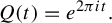
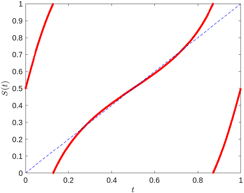
Let $Q:[0,1)\to \mathbb {T}$ be given by $Q(t)=e^{2\pi it}.$ Throughout, we identify $T:\mathbb {T}\to \mathbb {T}$ with $S:[0,1)\to [0,1)$ where S is given by $S(t)=(Q^{-1}TQ)(t).$ Figure 1 shows an example of one such map.

Remark 2.4. When $n=1$ , T is a Möbius transformation, and so some literature restricts the definition of a Blaschke product to $n\ge 2$ , but throughout this work we consider $n\ge 1.$

Figure 1

Plot of t versus $S(t)=(Q^{-1}TQ)(t)$ , where $T(z)=-(({z-0.4})/({1-0.4z}))^2, Q(t)=e^{2\pi i t}$ (color online).

Line graph of S of t versus t on a unit square. A thick red curve shows a periodic sigmoidal trend with discontinuities at t equals 0.13 and 0.87. A dashed blue diagonal line represents the identity function from 0,0 to 1,1.

Theorem 2.5. [Reference Pujals, Robert and Shub26, Proposition 1.2]

For $n\ge 2$ , let T be a Blaschke product of degree n. Then one of three mutually exclusive cases holds:

(1) T has $n+1$ fixed points on $\mathbb {T}$ , where one is attracting and the remaining n are expanding;
(2) T has $n-1$ expanding fixed points on $\mathbb {T}.\, T$ has one attracting fixed point $x\in D$ and another fixed point at $1/\bar {x}$ ;
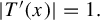
(3) T has $n+1$ fixed points on $\mathbb {T}$ where one fixed point x is indifferent, that is, ${|T'(x)|=1.}$

Proposition 2.6. [Reference Andersson1, Proposition 1.4]

For $x\in D$ and a continuous function $f:\mathbb {T}\to \mathbb {C}$ , let $\tilde {f}:D\to \mathbb {C}$ be given by

$$ \begin{align*}\tilde{f}(x)=\int_{\mathbb{T}}f(z)\frac{1-|x|^{2}}{|x-z|^{2}}\,dm(z).\end{align*} $$ StartLayout 1st Row ModifyingAbove f With tilde left parenthesis x right parenthesis equals integral Underscript double struck upper T Endscripts f left parenthesis z right parenthesis StartFraction 1 minus StartAbsoluteValue x EndAbsoluteValue squared Over StartAbsoluteValue x minus z EndAbsoluteValue squared EndFraction d m left parenthesis z right parenthesis period EndLayout

We call $\tilde {f}$ the harmonic extension of f to the disc and $P_{x}:=P_{x}(z)=({1-|x|^{2}})/({|z-x|^{2}})$ the Poisson kernel (associated to x).

Then $\tilde {f}$ has the following properties:

• $\tilde {f}$ is harmonic on $D;$ and
• for $z\in \mathbb {T}$ , $\lim _{r\nearrow 1}\tilde {f}(rz)=f(z).$

The next lemma follows from [Reference Stein and Shakarchi30, Lemma 8.1.3] and will be used in the proof of Lemma 4.2.

Lemma 2.7. If $\tilde {f}:D\to D$ is harmonic and $T:D\to D$ is holomorphic, then $\tilde {f}\circ T$ is harmonic.

The next theorem follows from [Reference Pujals, Robert and Shub26, Proposition 4.1], and we include a proof here for completeness.

Theorem 2.8. If T is a Blaschke product, $f\in C(\mathbb {T})$ and $x\in D$ , then

$$ \begin{align*}\int_{\mathbb{T}}f\circ T\cdot P_{x}\,dm=\int_{\mathbb{T}}f\cdot P_{T(x)}\,dm.\end{align*} $$

Proof. Let $f\in C(\mathbb {T}).$ Fix $x\in D.$ Then we have

$$ \begin{align*} \int_{\mathbb{T}} f\circ T\cdot P_{x}\,dm&=\widetilde{f\circ T}(x)\\&=\tilde{f}\circ T(x)\\&=\int_{\mathbb{T}} f\cdot P_{T(x)}\,dm, \end{align*} $$

StartLayout 1st Row 1st Column integral Underscript double struck upper T Endscripts f ring upper T dot upper P Subscript x d m 2nd Column equals ModifyingAbove f ring upper T With tilde left parenthesis x right parenthesis 2nd Row 1st Column Blank 2nd Column equals f overtilde ring upper T left parenthesis x right parenthesis 3rd Row 1st Column Blank 2nd Column equals integral Underscript double struck upper T Endscripts f dot upper P Subscript upper T left parenthesis x right parenthesis Baseline d m comma EndLayout

where the first and third lines follow from Proposition 2.6 and the second line from Lemma 2.7.

For a function $f:\mathbb {T}\to \mathbb {C}$ , we let $\|f\|_{\infty }:=\mathrm {ess}\sup _{z\in \mathbb {T}}|f(z)|.$ Lemmas 2.9 and 2.10 will be used in the proof of Theorem 1.2(i).

Lemma 2.9. Let $0<r<1$ and take $z_{0}\in \mathbb {T}.$ Then

$$ \begin{align*}\lim_{r\to1}\|P_{rz_{0}}\|_{\infty}=\infty.\end{align*} $$

Proof. Since $P_{rz_0}(z)=({1-|rz_{0}|^2})/({|z-rz_{0}|^2})=({1-r^2})/({|z-rz_{0}|^2})$ is continuous on $\mathbb {T}$ , it follows that

$$ \begin{align*}\|P_{rz_{0}}\|_{\infty}&=\frac{1-r^2}{\inf_{z\in\mathbb{T}}|z-rz_{0}|^2}\\&=\frac{1-r^2}{|z_{0}-rz_{0}|^2}\\&=\frac{1+r}{1-r}.\end{align*} $$

StartLayout 1st Row 1st Column StartMetric upper P Subscript r z 0 Baseline EndMetric Subscript infinity 2nd Column equals StartFraction 1 minus r squared Over inf Underscript z element of double struck upper T Endscripts StartAbsoluteValue z minus r z 0 EndAbsoluteValue squared EndFraction 2nd Row 1st Column Blank 2nd Column equals StartFraction 1 minus r squared Over StartAbsoluteValue z 0 minus r z 0 EndAbsoluteValue squared EndFraction 3rd Row 1st Column Blank 2nd Column equals StartFraction 1 plus r Over 1 minus r EndFraction period EndLayout

In the second line we have used the fact that $z_{0}$ is the closest point on $\mathbb {T}$ to $rz_{0}.$ Thus the claim follows.

Lemma 2.10. Take $x,y\in D.$ Then

$$ \begin{align*}\|P_{x}-P_{y}\|_{\infty}\le\frac{12|x-y|}{(1-|x|)^2(1-|y|)^2}.\end{align*} $$ StartMetric upper P Subscript x Baseline minus upper P Subscript y Baseline EndMetric Subscript infinity Baseline less than or equals StartFraction 12 StartAbsoluteValue x minus y EndAbsoluteValue Over left parenthesis 1 minus StartAbsoluteValue x EndAbsoluteValue right parenthesis squared left parenthesis 1 minus StartAbsoluteValue y EndAbsoluteValue right parenthesis squared EndFraction period

Proof. For $z\in \mathbb {T}$ we have

$$ \begin{align*} |P_{x}(z)-P_{y}(z)|&=\bigg|\frac{1-|x|^2}{|z-x|^2}-\frac{1-|y|^2}{|z-y|^2}\bigg|\\&\le\frac{(1-|x|^2)\|z-y|^2-|z-x|^2|+|z-x|^2\|y|^2-|x|^2|}{|z-x|^2|z-y|^2}\\&\le\frac{(1-|x|^2)|(z-y)^2-(z-x)^2|+|z-x|^2|y^2-x^2|}{|z-x|^2|z-y|^2}\\&=\frac{(1-|x|^2)|y-x|(|y+x-2z|+|z-x|^2|y+x|)}{|z-x|^2|z-y|^2}\\&\le\frac{12|x-y|}{(1-|x|)^2(1-|y|)^2}, \end{align*} $$

StartLayout 1st Row 1st Column StartAbsoluteValue upper P Subscript x Baseline left parenthesis z right parenthesis minus upper P Subscript y Baseline left parenthesis z right parenthesis EndAbsoluteValue 2nd Column equals StartAbsoluteValue StartFraction 1 minus StartAbsoluteValue x EndAbsoluteValue squared Over StartAbsoluteValue z minus x EndAbsoluteValue squared EndFraction minus StartFraction 1 minus StartAbsoluteValue y EndAbsoluteValue squared Over StartAbsoluteValue z minus y EndAbsoluteValue squared EndFraction EndAbsoluteValue 2nd Row 1st Column Blank 2nd Column less than or equals StartFraction left parenthesis 1 minus StartAbsoluteValue x EndAbsoluteValue squared right parenthesis StartMetric z minus y vertical bar Superscript 2 Baseline minus StartAbsoluteValue z minus x EndAbsoluteValue squared StartAbsoluteValue plus EndAbsoluteValue z minus x vertical bar Superscript 2 Baseline EndMetric y vertical bar Superscript 2 Baseline minus StartAbsoluteValue x EndAbsoluteValue squared vertical bar Over StartAbsoluteValue z minus x EndAbsoluteValue squared StartAbsoluteValue z minus y EndAbsoluteValue squared EndFraction 3rd Row 1st Column Blank 2nd Column less than or equals StartFraction left parenthesis 1 minus StartAbsoluteValue x EndAbsoluteValue squared right parenthesis StartAbsoluteValue left parenthesis z minus y right parenthesis squared minus left parenthesis z minus x right parenthesis squared EndAbsoluteValue plus StartAbsoluteValue z minus x EndAbsoluteValue squared StartAbsoluteValue y squared minus x squared EndAbsoluteValue Over StartAbsoluteValue z minus x EndAbsoluteValue squared StartAbsoluteValue z minus y EndAbsoluteValue squared EndFraction 4th Row 1st Column Blank 2nd Column equals StartFraction left parenthesis 1 minus StartAbsoluteValue x EndAbsoluteValue squared right parenthesis StartAbsoluteValue y minus x EndAbsoluteValue left parenthesis StartAbsoluteValue y plus x minus 2 z EndAbsoluteValue plus StartAbsoluteValue z minus x EndAbsoluteValue squared StartAbsoluteValue y plus x EndAbsoluteValue right parenthesis Over StartAbsoluteValue z minus x EndAbsoluteValue squared StartAbsoluteValue z minus y EndAbsoluteValue squared EndFraction 5th Row 1st Column Blank 2nd Column less than or equals StartFraction 12 StartAbsoluteValue x minus y EndAbsoluteValue Over left parenthesis 1 minus StartAbsoluteValue x EndAbsoluteValue right parenthesis squared left parenthesis 1 minus StartAbsoluteValue y EndAbsoluteValue right parenthesis squared EndFraction comma EndLayout

where the second, third and last lines follow by applying the triangle inequality.

Definition 2.11. Consider a point $x\in \overline {D}.$ We define the probability measure $\mu _{x}$ as follows.

• If $x\in D$ , then let $\mu _{x}$ be the measure satisfying ${d\mu _{x}}/{dm}=P_{x}$ , where m denotes the Lebesgue measure.
• If $x\in \mathbb {T}$ , let $\mu _{x}=\delta _{x}$ , the Dirac measure.

Remark 2.12. [Reference Pujals, Robert and Shub26]

Let $\phi _{x}$ be the Möbius transformation mapping $0$ to x, $\phi _{x}(z)=({z+x})/({1+\bar {x}z})$ . For $x\in D$ , $\mu _{x}$ in Definition 2.11 is equivalently given by ${\mu _{x}=(\phi _{x})_*(m)}$ , the pushforward of m with respect to $\phi _{x}$ .

If $x\in \overline {D}$ is a fixed point of a Blaschke product T, then it follows from Definition 2.11 and Theorem 2.8 that $\mu _{x}$ is T-invariant, that is, $(T)_{*}(\mu _{x})=\mu _{x}.$

The next theorem follows as a consequence of [Reference Pujals, Robert and Shub26, Theorem 1.2].

Theorem 2.13. Let T be a Blaschke product of degree $n\ge 2$ with fixed point $x\in D$ . Let $\mu _{x}$ be as in Definition 2.11. The measure-theoretic entropy of T with respect to $\mu _{x}$ is given by

$$ \begin{align*}h_{\mu_{x}}(T)=\int_{\mathbb{T}}\log|T'(z)|\,d\mu_{x}.\end{align*} $$

2.2 Map cocycles and their measure-theoretic entropy

In this section, we give relevant definitions and results relating to map cocycles and their measure-theoretic entropy that will be used throughout this work.

Definition 2.14. (Map cocycle)

Let $(\Omega ,\mathcal {F},\mathbb {P})$ be a probability space. Let $\mathcal {T}:=(T_{\omega })_{\omega \in \Omega }$ be a family of measurable transformations of $(X,\mathcal {B}).$ A map cocycle is a tuple ${\mathcal {R}=(\mathcal {T},\sigma )}$ where $\sigma :\Omega \to \Omega $ is an invertible, ergodic, measure-preserving transformation of $(\Omega ,\mathcal {F},\mathbb {P}).$ We call $(\Omega , \mathcal {F},\mathbb {P}, \sigma )$ the base dynamical system. We will simply write $\mathcal {T}$ when $\sigma $ is clear from the context.

Throughout we will refer to a $\mathcal {T}$ -invariant measure (or random invariant measure), given by the follow definition.

Definition 2.15. ( $\mathcal {T}$ -invariant measure)

Let $(\mathcal {T},\sigma )$ be a map cocycle. Let $\mu $ be a measure on $\Omega \times \mathbb {T}$ which has disintegration $\{\mu _{\omega }\}_{\omega \in \Omega }$ with respect to $\mathbb {P}.$ We call $\mu $ a $\mathcal {T}$ -invariant measure if $\mu _{\omega }$ is a probability measure, $\omega \mapsto \mu _{\omega }$ is measurable and for $\mathbb {P}$ -a.e. $\omega \in \Omega $ ,

$$ \begin{align*} (T_{\omega})_{*}(\mu_{\omega})=\mu_{\sigma\omega}. \end{align*} $$

The following result due to Bogenschütz, adapted to our setting, tells us that the metric entropy of a random dynamical system is given as the sum of its so-called fibre entropy and the entropy of its base dynamical system.

Lemma 2.16. [Reference Bogenschütz and Crauel6, Corollary 1]

Let $(\Omega ,\mathcal {F},\mathbb {P},\sigma )$ be a dynamical system where ${\sigma :\Omega \to \Omega }$ is an ergodic invertible $\mathbb {P}$ -preserving transformation. Let $(\mathcal {T}, \sigma )$ be a map cocycle. Furthermore, let $\mu $ be a $\mathcal {T}$ -invariant measure. For a partition $\mathcal {P}$ of X, let

$$ \begin{align*}h^{\mathrm{fib}}_{\mu}(\mathcal{T};\mathcal{P})=\lim_{n\to\infty}\frac{1}{n}\int_{\Omega} H_{\mu_{\omega}}\bigg(\bigvee_{i=0}^{n-1}T^{-i}_{\omega}\mathcal{P}\bigg)\,d\mathbb{P}(\omega),\end{align*} $$

h Subscript mu Superscript fib Baseline left parenthesis script upper T semicolon script upper P right parenthesis equals limit Underscript n right arrow infinity Endscripts StartFraction 1 Over n EndFraction integral Underscript normal upper Omega Endscripts upper H Subscript mu Sub Subscript omega Subscript Baseline left parenthesis or Underscript i equals 0 Overscript n minus 1 Endscripts upper T Subscript omega Superscript negative i Baseline script upper P right parenthesis d double struck upper P left parenthesis omega right parenthesis comma

where $H_{\mu _{\omega }}(\mathcal {P})=-\sum _{A\in \mathcal {P}}\mu _{\omega }(A)\log \mu _{\omega }(A)$ , and let $h_{\mu }^{\mathrm {fib}}(\mathcal {T})=\sup \{h^{\mathrm {fib}}_{\mu }(\mathcal {T};\mathcal {P})\}$ where the supremum is taken over all finite partitions $\mathcal {P}$ of $X.$ If $\mathcal {F}$ is countably generated $(\text {mod }0)$ , then

$$ \begin{align*}h_{\mu}(\mathcal{T})=h_{\mu}^{\mathrm{fib}}(T)+h_{\mathbb{P}}(\sigma).\end{align*} $$

Definition 2.17. A measurable function $T:X\to X$ on a measure space $(X,\mathcal {B},\mu )$ is said to be non-singular with respect to $\mu $ if $\mu (T^{-1}(B))=0$ for all $B\in \mathcal {B}$ such that $\mu (B)=0.$

Definition 2.18. (Lasota–Yorke map)

$T:[0,1]\to [0,1]$ is called a Lasota–Yorke map if there exists a finite subdivision $0=b_{0}<b_{1}<\cdots <b_{n}=1$ such that for each restriction $T_{i}$ of T to any subinterval $(b_{i-1}, b_{i}),\ i=1,\ldots ,n$ :

(1) $T_{i}$ is a homeomorphism on its image; and
(2) $T_{i}$ is non-singular with respect to the Lebesgue measure.

Lemma 2.19. (Duality relation)

Let $\mathcal {L}_{T}$ be as in Definition 1.1. Let $f\in C(\mathbb {T})$ , $g\in L^{\infty }(\mathbb {T}).$ Then $\mathcal {L}_{T}$ satisfies the duality relation

$$ \begin{align*}\int_{\mathbb{T}}f\cdot g\circ T\,dm=\int_{\mathbb{T}}g\cdot\mathcal{L}_{T}f\,dm.\end{align*} $$

Definition 2.20. (Variation)

For a function $f:[0,1]\to \mathbb {R}$ , the variation of f is given by

$$ \begin{align*}\mathrm{var}(f):=\sup_{\mathcal{P}}\sum_{j=1}^{n}|f(b_{j})-f(b_{j-1})|\end{align*} $$ StartLayout 1st Row var left parenthesis f right parenthesis colon equals sup Underscript script upper P Endscripts sigma summation Underscript j equals 1 Overscript n Endscripts StartAbsoluteValue f left parenthesis b Subscript j Baseline right parenthesis minus f left parenthesis b Subscript j minus 1 Baseline right parenthesis EndAbsoluteValue EndLayout

where $\mathcal {P}=(0=b_{0}<b_{1}<\cdots <b_{n}=1)$ is a finite partition of $[0,1].$

The following theorem gives sufficient conditions for the existence of a limiting random invariant measure for a class of random maps.

Theorem 2.21. [Reference Buzzi7]

Let $\sigma $ be an invertible, ergodic, measure-preserving transformation of a probability space $(\Omega , \mathcal {F}, \mathbb {P}).$ Suppose a random Lasota–Yorke map $\mathcal {T}:=(T_{\omega })_{\omega \in \Omega }$ satisfies the following conditions:

(1) $\omega {\kern-1pt}\mapsto{\kern-1pt} (\inf _{x\in [0,1]\backslash \{b_{0},\ldots ,b_{d_{\omega }}\}}|T_{\omega }'(x)|,\mathrm {var}(1/|T_{\omega }'|), d_{\omega }, b_{0},\ldots ,b_{d_{\omega }})$ is measurable on $\Omega $ ;
(2) $\lim _{K\to \infty }\int _{\Omega }\log \min (\inf _{x\in [0,1]\backslash \{b_{0},\ldots ,b_{d_{\omega }}\}}|T'(x)|, K)\,d\mathbb {P}(\omega )>0$ ;
(3) $\int _{\Omega }\log ^{+}({d_{\omega }}/{\inf _{x\in [0,1]\backslash \{b_{0},\ldots ,b_{d_{\omega }}\}}|T'(x)|})\,d\mathbb {P}(\omega )<\infty $ ;
(4) $\int _{\Omega }\log ^{+}\mathrm {var}({1}/{|T_{\omega }'|})\,d\mathbb {P}(\omega )<\infty $ ;
(5) for every non-trivial $I\subset [0,1]$ and $\mathbb {P}$ -a.e. $\omega \in \Omega $ there exists $n_{c}:=n_{c}(\omega )$ such that for all $n\ge n_{c}$ , $\mathrm {ess}\inf _{x\in [0,1]}(\mathcal {L}_{\omega }^{(n)}1_{I}(x))>0$ , where $1_{I}$ is the characteristic function of I and $\mathcal {L}_{\omega }^{(n)}:=\mathcal {L}_{\sigma ^{n-1}\omega }\circ \cdots \circ \mathcal {L}_{\omega }.$

Then the following assertions hold.

(i) There is a density h on $\Omega \times [0,1]$ , such that $\int _{0}^{1}h_{\omega }dm=1$ and for $\mathbb {P}$ -a.e. $\omega \in \Omega $ ,
$$ \begin{align*}\mathcal{L}_{\omega}h_{\omega}=h_{\sigma\omega}.\end{align*} $$

Moreover, h is unique modulo m and $\mathrm {var}(h_{\omega })<\infty $ for $\mathbb {P}$ -a.e. $\omega \in \Omega $ ,
(ii) There exists $\rho <1$ such that for all $h_{*}:X\to [0,\infty )$ with bounded variation and $\|h_{*}\|_{1}=1$ , for $\mathbb {P}$ -a.e. $\omega \in \Omega $ , there is $n_{0}(\omega ):=n_{0}$ such that for all $n\ge n_{0}$ ,
$$ \begin{align*}\|\mathcal{L}_{\sigma^{-n}\omega}^{(n)}h_{*}-h_{\omega}\|_{\infty}\le\rho^n.\end{align*} $$

The following theorem is a corollary of [Reference Bogenschütz5, Theorem 6.1].

Theorem 2.22. Let $(\mathcal {T},\sigma )$ be a map cocycle with the family of transfer operators $(\mathcal {L}_{\omega })_{\omega \in \Omega }$ as in Definition 1.1. Then

$$ \begin{align*}0=\sup_{\mu\ \mathcal{T}\text{-}\mathrm{inv.}}\bigg\{h_{\mu}^{\mathrm{fib}}(\mathcal{T})-\int_{\Omega\times X}\log|T_{\omega}'| \,d\mu\bigg\}.\end{align*} $$ 0 equals sup Underscript mu script upper T minus inv period Endscripts left brace h Subscript mu Superscript fib Baseline left parenthesis script upper T right parenthesis minus integral Underscript normal upper Omega times upper X Endscripts log StartAbsoluteValue upper T Subscript omega Superscript prime Baseline EndAbsoluteValue d mu right brace period

Definition 2.23. (Blaschke product cocycle)

Let $\sigma $ be an invertible, ergodic, measure-preserving transformation of a probability space $(\Omega , \mathcal {F}, \mathbb {P}).$ Let $\mathcal {T}=(T_{\omega })_{\omega \in \Omega }$ , where for each $\omega \in \Omega $ , we let $T_{\omega }:\hat {\mathbb {C}}\to \hat {\mathbb {C}}$ be given by

$$ \begin{align*}T_{\omega}(z)=\rho_{\omega}\prod_{i=1}^{d_{\omega}}\frac{z-a_{i,\omega}}{1-\bar{a}_{i,\omega}z},\end{align*} $$ upper T Subscript omega Baseline left parenthesis z right parenthesis equals rho Subscript omega Baseline product Underscript i equals 1 Overscript d Subscript omega Baseline Endscripts StartFraction z minus a Subscript i comma omega Baseline Over 1 minus a overbar Subscript i comma omega Baseline z EndFraction comma

upper T Subscript omega Baseline left parenthesis z right parenthesis equals rho Subscript omega Baseline product Underscript i equals 1 Overscript d Subscript omega Baseline Endscripts StartFraction z minus a Subscript i comma omega Baseline Over 1 minus a overbar Subscript i comma omega Baseline z EndFraction comma

where $\mathrm{d}:\Omega \to \mathbb {N},\rho :\Omega \to \mathbb {T}$ are measurable and for each $j\ge 1$ such that $\Omega _{j}:=\{\omega \in \Omega :\mathrm{d}_{\omega }=j\}$ is non-empty, $a:\Omega _{j}\to D^{j}, D^{j}:=\underbrace {D\times \cdots \times D}_{j \text { times}}$ a colon normal upper Omega Subscript j Baseline right arrow upper D Superscript j Baseline comma upper D Superscript j Baseline colon equals ModifyingBelow upper D times midline horizontal ellipsis times upper D With bottom brace Underscript j times Endscripts is measurable. The Blaschke product cocycle is $(\mathcal {T}, \sigma )$ , or simply $\mathcal {T}.$ We let ${T_{\omega }^{(n)}{\kern-1pt}={\kern-1pt}T_{\sigma ^{n-1}\omega }\circ \cdots \circ T_{\omega }}$ and $T_{\sigma ^{-n}\omega }^{(n)}=T_{\sigma ^{-1}\omega }\circ \cdots \circ T_{\sigma ^{-n}\omega }.$

In Theorem 1.3, we consider the family $\mathcal {T}_{\theta }:=(\theta T_{\omega })_{\omega \in \Omega }.$ For all $\omega \in \Omega $ , we let $T_{\omega ,\theta }:=\theta T_{\omega }$ and $T_{\sigma ^{-n}\omega ,\theta }^{(n)}=T_{\sigma ^{-1}\omega ,\theta }\circ \cdots \circ T_{\sigma ^{-n}\omega ,\theta }.$ When $\theta =1$ , we will write $\mathcal {T}$ and $T_{\sigma ^{-n}\omega }^{(n)}.$

The following theorem gives a sufficient condition on a Blaschke product cocycle for the existence of measurable $x:\Omega \to D$ such that for $\mathbb {P}$ -a.e. $\omega \in \Omega $ and all $z\in D$ , $x_{\omega }=\lim _{n\to \infty }T_{\sigma ^{-n}\omega }^{(n)}(z).$ We call $(x_{\omega })_{\omega \in \Omega }$ a random fixed point.

Theorem 2.24. [Reference González-Tokman and Quas15, Theorem 1(1)]

Let $\sigma $ be an invertible ergodic measure-preserving transformation of a probability space $(\Omega ,\mathbb {P}).$ Let $r_{T}(R)=\sup _{|z|=R}|T(z)|.$ We denote $r_{\mathcal {T}}(R)=\mathrm {ess}\sup _{\omega \in \Omega }r_{T_{\omega }}(R).$ Let $R<1$ and let $\mathcal {T}=(T_{\omega })_{\omega \in \Omega }$ be a Blaschke product cocycle, depending measurably on $\omega $ , satisfying $r:=r_{\mathcal {T}}(R)<R.$ Then there exists a measurable map $x:\Omega \to \bar {D}_{r}$ (with $x(\omega )$ written as $x_{\omega }$ ), such that $T_{\omega }(x_{\omega })=x_{\sigma \omega }$ . Furthermore, for all $z\in D_{R}$ , $T_{\sigma ^{-N}\omega }^{(N)}(z):=T_{\sigma ^{-1}\omega }\circ \cdots \circ T_{\sigma ^{-N}\omega }(z)\to x_{\omega }$ as $N\to \infty .$

Remark 2.25. The hypotheses of Theorem 2.24 ensure the existence of a random fixed point through uniform contraction $D_{R}$ into a smaller disc $D_{r}.$ In particular, this means that, for all $\omega \in \Omega $ , $\inf _{z\in \mathbb {T}}|T_{\omega }'(z)|\ge ({\log r})/({\log R})>1$ [Reference Tischler31, Theorem 2]. In contrast, Theorem 1.2 requires expansion on average, allowing for some maps that are not only not uniformly expanding, but also have an attracting fixed point on the circle (see Example 5.1).

3 Measure-theoretic entropy for an admissible Blaschke product cocycle

In this section, we obtain a formula for the measure-theoretic entropy of an admissible Blaschke product cocycle $\mathcal {T}.$

For $B\subset \mathbb {T}$ , let $m(B)$ denote the normalized Lebesgue measure of B, so that $m(\mathbb {T})=1$ .

Definition 3.1. (Admissible Blaschke product cocycle)

Consider a Blaschke product cocycle $(\mathcal {T},\sigma ).$ Let $d_{\omega }:=\deg (T_{\omega }).$ Suppose the following conditions hold:

(1) $\omega \mapsto (\inf _{z\in \mathbb {T}}|T_{\omega }'(z)|, \mathrm {var}({1}/({|T_{\omega }'|})))$ is measurable on $\Omega ;$
(2) $\log \inf _{z\in \mathbb {T}}|T_{\omega }'(z)|\in L^{1}(\mathbb {P})\text { and }$ $\int _{\Omega }\log \inf _{z\in \mathbb {T}}|T_{\omega }'(z)|\,d\mathbb {P}(\omega )>0;$
(3) $\int _{\Omega }\log ({d_{\omega }}/({\inf _{z\in \mathbb {T}} |T_{\omega }'(z)|}))\,d\mathbb {P}(\omega )<\infty ;$ and
(4) $\int _{\Omega }\log ^{+}\int _{\mathbb {T}} |{T"}/{(T')^2} |\,dm\,d\mathbb {P}(\omega )<\infty .$

Then $(\mathcal {T}, \sigma )$ , or simply $\mathcal {T}$ , is called an admissible Blaschke product cocycle.

Remark 3.2. These conditions ensure that the cocycle conjugated to $[0,1)$ , given by $\tilde {T}_{\omega }=Q^{-1}\circ T_{\omega }\circ Q$ , where $Q(x)=e^{2\pi i x}$ , satisfies the hypotheses of Theorem 2.21. For all $\omega \in \Omega $ , $\lim _{K\to \infty }\log \min (K, \inf _{z\in \mathbb {T}}|T_{\omega }'(z)|)=\log \inf _{z\in \mathbb {T}}|T_{\omega }'(z)|$ and, since $\log \inf _{z\in \mathbb {T}}|T_{\omega }'(z)|$ is integrable (condition (2)), Theorem 2.21 $(2)$ holds by dominated convergence. In addition, condition (2) in this setting implies Theorem 2.21 $(5)$ (see Lemma 3.3). Conditions (1), (3) and (4) are equivalent to the corresponding conditions in Theorem 2.21 (see the proof of Theorem 1.2(ii)).

The proof of the following lemma follows similarly to [Reference Dragičević, Hafouta and Sedro11, Example 6].

Lemma 3.3. Take non-trivial arc $A\subset \mathbb {T}$ such that $m(A)<1.$ Suppose $\mathcal {T}$ is an admissible Blaschke product cocycle. Then, for $\mathbb {P}$ -a.e. $\omega \in \Omega $ , there exists $n_{c}(\omega , A):=n_{c}(\omega )$ such that for every $n\ge n_{c}(\omega )$ we have $m(T_{\omega }^{(n)}(A))=1.$

Proof. The measure m can be thought of as the normalized arc length measure on the unit circle. Assuming $m(T_{\omega }^{(n)}(A))<1$ , we have

$$ \begin{align*}m(T_{\omega}^{(n)}(A))\ge\inf_{z\in\mathbb{T}}|(T_{\omega}^{(n)})'(z)|m(A)\ge m(A)\prod_{k=0}^{n-1}\inf_{z\in\mathbb{T}}|T_{\sigma^{k}\omega}'(z)|.\end{align*} $$

StartLayout 1st Row m left parenthesis upper T Subscript omega Superscript left parenthesis n right parenthesis Baseline left parenthesis upper A right parenthesis right parenthesis greater than or equals inf Underscript z element of double struck upper T Endscripts StartAbsoluteValue left parenthesis upper T Subscript omega Superscript left parenthesis n right parenthesis Baseline right parenthesis prime left parenthesis z right parenthesis EndAbsoluteValue m left parenthesis upper A right parenthesis greater than or equals m left parenthesis upper A right parenthesis product Underscript k equals 0 Overscript n minus 1 Endscripts inf Underscript z element of double struck upper T Endscripts StartAbsoluteValue upper T prime Subscript sigma Sub Superscript k Subscript omega Baseline left parenthesis z right parenthesis EndAbsoluteValue period EndLayout

By the Birkhoff ergodic theorem, for $\mathbb {P}$ -a.e. $\omega \in \Omega $ ,

$$ \begin{align*}\lim_{n\to\infty}\frac{1}{n}\sum_{k=0}^{n-1}\inf_{z\in\mathbb{T}}|T_{\sigma^{k}\omega}'(z)|=\int_{\Omega}\log\inf_{z\in\mathbb{T}}|T_{\omega}'(z)|\,d\mathbb{P}(\omega)=:\Lambda>0.\end{align*} $$

StartLayout 1st Row limit Underscript n right arrow infinity Endscripts StartFraction 1 Over n EndFraction sigma summation Underscript k equals 0 Overscript n minus 1 Endscripts inf Underscript z element of double struck upper T Endscripts StartAbsoluteValue upper T prime Subscript sigma Sub Superscript k Subscript omega Baseline left parenthesis z right parenthesis EndAbsoluteValue equals integral Underscript normal upper Omega Endscripts log inf Underscript z element of double struck upper T Endscripts StartAbsoluteValue upper T prime Subscript omega Baseline left parenthesis z right parenthesis EndAbsoluteValue d double struck upper P left parenthesis omega right parenthesis equals colon normal upper Lamda greater than 0 period EndLayout

We choose $n_{0}:=n_{0}(\omega )$ sufficiently large such that $({1}/{n_{0}})\sum _{k=0}^{n_{0}-1}\inf _{z\in \mathbb {T}}|T_{\sigma ^{k}\omega }'(z)|\ge \Lambda /2.$ Thus, for all $n\ge n_{0}$ , we have

$$ \begin{align*}\prod_{k=0}^{n-1}\inf_{z\in\mathbb{T}}|T_{\sigma^{k}\omega}'(z)|\ge e^{n\Lambda/2}.\end{align*} $$ product Underscript k equals 0 Overscript n minus 1 Endscripts inf Underscript z element of double struck upper T Endscripts StartAbsoluteValue upper T prime Subscript sigma Sub Superscript k Subscript omega Baseline left parenthesis z right parenthesis EndAbsoluteValue greater than or equals e Superscript n normal upper Lamda divided by 2 Baseline period

product Underscript k equals 0 Overscript n minus 1 Endscripts inf Underscript z element of double struck upper T Endscripts StartAbsoluteValue upper T prime Subscript sigma Sub Superscript k Subscript omega Baseline left parenthesis z right parenthesis EndAbsoluteValue greater than or equals e Superscript n normal upper Lamda divided by 2 Baseline period

Now, taking $n_{c}(\omega )=\max (n_{0}(\omega ),\lceil -({2}/{\Lambda })\log m(A)\rceil )$ it follows that $m(T_{\omega }^{(n)}(A))=1$ for $n\ge n_{c}(\omega ).$

Lemma 3.4. Assume $(\mathcal {T}, \sigma )$ is a Blaschke product cocycle. Suppose there is measurable $x:\Omega \to D$ such that $T_{\omega }(x_{\omega })=x_{\sigma \omega }.$ Suppose $\mu $ is a measure on $\Omega \times X$ with disintegration $\{\mu _{\omega }\}_{\omega \in \Omega }$ and marginal $\mathbb {P}$ with respect to $\Omega $ such that $({d\mu _{\omega }}/{dm}):=P_{x_{\omega }}.$ Then $\{\mu _{\omega }\}_{\omega \in \Omega }$ is a $\mathcal {T}-$ invariant measure.

Proof. Take $f\in C(\mathbb {T}).$ We have

$$ \begin{align*} \int_{\mathbb{T}}f\circ T_{\omega}\,d\mu_{\omega}&=\int_{\mathbb{T}}f\circ T_{\omega}P_{x_{\omega}}\,dm\\&=\int_{\mathbb{T}} fP_{T_{\omega}(x_{\omega})}\,dm\\&=\int_{\mathbb{T}} fP_{x_{\sigma\omega}}\,dm\\&=\int_{\mathbb{T}} f\,d\mu_{\sigma\omega}, \end{align*} $$

StartLayout 1st Row 1st Column integral Underscript double struck upper T Endscripts f ring upper T Subscript omega Baseline d mu Subscript omega 2nd Column equals integral Underscript double struck upper T Endscripts f ring upper T Subscript omega Baseline upper P Subscript x Sub Subscript omega Baseline d m 2nd Row 1st Column Blank 2nd Column equals integral Underscript double struck upper T Endscripts f upper P Subscript upper T Sub Subscript omega Subscript left parenthesis x Sub Subscript omega Subscript right parenthesis Baseline d m 3rd Row 1st Column Blank 2nd Column equals integral Underscript double struck upper T Endscripts f upper P Subscript x Sub Subscript sigma omega Baseline d m 4th Row 1st Column Blank 2nd Column equals integral Underscript double struck upper T Endscripts f d mu Subscript sigma omega Baseline comma EndLayout

where the second line follows from Theorem 2.8.

We show that the conditions for an admissible Blaschke product cocycle can be identified with the hypotheses of Theorem 2.21 and use this result to describe the unique acim for such a cocycle.

Proof of Theorem 1.2(ii).

Let $(\mathcal {T}, \sigma )$ be an admissible Blaschke product cocycle as in Definition 3.1.

Since each Blaschke product $T_{\omega }$ is a $d_{\omega }$ -to-one local homeomorphism, it follows that Definition 2.18(1) is satisfied. Definition 2.18(2) is satisfied since any Blaschke product T is a local diffeomorphism and thus non-singular with respect to Lebesgue [Reference de Faria and Guarino10].

Next we check the conditions of Theorem 2.21. Let $S_{\omega }=Q^{-1}T_{\omega }Q$ as in Definition 2.2. First note that $|{dS_{\omega }(t)}/{dt}|=|{dT_{\omega }(z)}/{dz}|$ .

From $|{dS_{\omega }(t)}/{dt}|=|{dT_{\omega }(z)}/{dz}|$ , it follows that $\mathrm {var}({1}/{|T_{\omega }'|})=\int _{\mathbb {T}}|{T_{\omega }"}/\, {(T_{\omega }')^2}|\,dm$ . Thus, Definition 3.1(4) is equivalent to Theorem 2.21(4).

Lastly, Lemma 3.3 implies Theorem 2.21(5). Thus, Theorem 1.2(ii) follows from Theorem 2.21.

Proof of Theorem 1.2(i).

Step 1 (Identification with Poisson kernel): Take $h^{*}=1.$ From Theorem 2.21, it follows that for $\mathbb {P}$ -a.e. $\omega \in \Omega $ there exists $h_{\omega }$ of bounded variation such that $\lim _{n\to \infty }\mathcal {L}_{\sigma ^{-n}\omega }^{(n)}1=h_{\omega }.$

From Lemma 2.19 and Lemma 2.8, we have

$$ \begin{align*}\int_{\mathbb{T}}f\cdot\mathcal{L}_{\sigma^{-n}\omega}^{(n)}1\,dm=\int_{\mathbb{T}}f\circ T_{\sigma^{-n}\omega}^{(n)}\,dm=\int_{\mathbb{T}} fP_{T_{\sigma^{-n}\omega}^{(n)}(0)}\,dm\end{align*} $$

for all $f\in C(\mathbb {T}).$ It follows that $\text { for all } n\in \mathbb {N}$ , $\mathcal {L}_{\sigma ^{-n}\omega }^{(n)}1=P_{T_{\sigma ^{-n}\omega }^{(n)}(0)}$ and thus from Theorem 2.21(ii) that $\lim _{n\to \infty }P_{T_{\sigma ^{-n}\omega }^{(n)}(0)}=h_{\omega }$ in $L^{\infty }.$

Step 2 (Extraction of a convergent subsequence): Now we will show for $\mathbb {P}$ -a.e. $\omega \in \Omega $ the existence of the limit $y_{\omega }=\lim _{n\to \infty }T_{\sigma ^{-n}\omega }^{(n)}(0)$ , and that $h_{\omega }=P_{y_{\omega }}.$ Consider the sequence $T_{\sigma ^{-n}\omega }^{(n)}(0)\subset D.$ This must have a convergence subsequence. In particular, there must be a subsequence $(n_{\omega ,k}):=(n_{k})$ such that $\lim _{k\to \infty }T_{\sigma ^{-n_{k}}\omega }^{(n_{k})}(0)= y_{\omega }\in \bar {D}.$

Suppose that $y_{\omega }\in \mathbb {T}$ , and so $|T_{\sigma ^{-n}\omega }^{(n)}(0)|\to 1.$ From Lemma 2.9, it follows that $\|h_{\omega }\|_{\infty }=\lim _{n\to \infty }\|P_{T_{\sigma ^{-n}\omega }^{(n)}(0)}\|_{\infty }=\infty .$ This can only happen on $\mathbb {P}$ measure 0, since $h_{\omega }$ is of bounded variation for $\mathbb {P}$ -a.e. $\omega \in \Omega $ , in particular $\|h_{\omega }\|_{\infty }<\infty .$ Thus, we must have $y_{\omega }\in D$ for $\mathbb {P}$ -a.e. $\omega \in \Omega .$

Step 3 (Uniqueness of the random fixed point): If $y_{\omega }\in D$ , then from Lemma 2.10,

$$ \begin{align*}\lim_{k\to\infty}|T_{\sigma^{-n_{k}}\omega}^{(n_{k})}(0)-y_{\omega}|=0\implies \lim_{k\to\infty}\|P_{T_{\sigma^{-n_{k}}\omega}^{(n_{k})}(0)}-P_{y_{\omega}}\|_{\infty}=0.\end{align*} $$

Furthermore, the uniqueness of $h_{\omega }$ gives $\lim _{n\to \infty }T_{\sigma ^{-n}\omega }^{(n)}(0)=y_{\omega }.$ For fixed $z\in D$ , taking $h_{*}=P_{z}$ gives $\lim _{n\to \infty }T_{\sigma ^{-n}\omega }^{(n)}(z)=y_{\omega }$ , and thus (i) holds.

We call $(y_{\omega })_{\omega \in \Omega }$ a random fixed point of $\mathcal {T}.$

Step 4 (Construction and invariance of $\mu $ ): Lastly, let $\mu $ be the measure with disintegration $\{\mu _{\omega }\}_{\omega \in \Omega }$ with respect to $\mathbb {P}$ , where ${d\mu _{\omega }}/{dm}=P_{y_{\omega }}.$ It follows from Lemma 3.4 that $\{\mu _{\omega }\}_{\omega \in \Omega }$ is $\mathcal {T}$ -invariant.

We now give the measure-theoretic entropy of $\mathcal {T}$ with respect to $\mu .$

Corollary 3.5. Let $\mathcal {T}$ be an admissible random Blaschke product with $\mu $ its random acim as in Theorem 1.2. Then the metric entropy with respect to $\mu $ of $\mathcal {T}$ is given by

$$ \begin{align*}h_{\mu}(\mathcal{T})=h_{\mathbb{P}}(\sigma)+\int_{\Omega}\int_{\mathbb{T}}\log|T^{\prime}_{\omega}|\,d\mu_{\omega}\,d\mathbb{P}(\omega).\end{align*} $$

Proof. From Lemma 2.16, it follows that

$$ \begin{align*}h_{\mu}(\mathcal{T})=h^{\mathrm{fib}}_{\mu}(\mathcal{T})+h_{\mathbb{P}}(\sigma).\end{align*} $$

By Theorem 2.22, $\sup _{\mu _{0}\text { }\mathcal {T}\text{-}\mathrm {inv.}}(h^{\mathrm {fib}}_{\mu _{0}}(\mathcal {T})+\int _{\Omega \times \mathbb {T}}-\log |T^{\prime }_{\omega }|\,d\mu _{0})=0.$ Thus, with random acim $\mu $ as in Theorem 1.2,

$$ \begin{align*}h_{\mu}^{\mathrm{fib}}(\mathcal{T})=\int_{\mathbb{T}\times\Omega}\log|T^{\prime}_{\omega}|\,d\mu=\int_{\Omega}\int_{\mathbb{T}}\log|T^{\prime}_{\omega}|\,d\mu_{\omega}\,d\mathbb{P}(\omega).\end{align*} $$

Thus the claim follows.

Example 3.6. Let $\mathcal {T}$ be a Blaschke product cocycle. Let $A_{\omega }=\sum _{i=1}^{d_{\omega }}(({1-|a_{i,\omega }|})/ ({1+|a_{i,\omega }|})).$ Suppose $\mathcal {T}$ satisfies the following assumptions:

(1) $\int _{\Omega }\log A_{\omega }\,d\mathbb {P}(\omega )>0;$
(2) $\int _{\Omega }\log ({d_{\omega }}/{A_{\omega }})\,d\mathbb {P}(\omega )<\infty ;$ and
(3) $\int _{\Omega }\log ({1}/({(1-\max _{k=1,\ldots ,d_{\omega }}|a_{k,\omega }|)A_{\omega }}))\,d\mathbb {P}(\omega )<\infty .$

Then the hypotheses of Theorem 1.2 hold. Indeed, it follows from [Reference Martin22] that $\inf _{z\in \mathbb {T}}|T_{\omega }'(z)|\ge \sum _{i=1}^{d_{\omega }}(({1-|a_{i,\omega }|})/({1+|a_{i,\omega }|}))$ , and so (1) gives Definition 3.1(2), (2) gives Definition 3.1(3). From applying the triangle inequality, it follows that (3) gives Definition 3.1(4).

4 Average entropy over a family of admissible Blaschke product cocycles

Let $\mathcal {T}$ be an admissible Blaschke product cocycle over $\sigma $ . For fixed $\theta \in \mathbb {C}$ , let $\mathcal {T}_{\theta }:=(\theta T_{\omega })_{\omega \in \Omega }.$ In this section, we obtain a formula for the average metric entropy over $\theta \in \mathbb {T}$ for the family of cocycles $(\mathcal {T}_{\theta })_{\theta \in \mathbb {T}}.$ This allows us to obtain information on the entropy without knowledge of particular orbits, in particular, without needing to find explicitly the invariant measure for each $\mathcal {T}_{\theta }.$

Let $T_{\omega , \theta }:=\theta T_{\omega }.$ The next lemma follows as in the deterministic case in [Reference Pujals, Robert and Shub26, Proposition 4.3]. We include the proof for completeness.

Lemma 4.1. Let $f:\mathbb {T}\to \mathbb {C}$ be a continuous function. Then, for all $n\in \mathbb {N}, \omega \in \Omega $ , $\int _{\mathbb {T}}\int _{\mathbb {T}} f\circ T_{\sigma ^{-n}\omega ,\theta }^{(n)} \,dm\,d\theta =\int _{\mathbb {T}}f\,dm.$

Proof. First, consider the inner integral. Recall that for a continuous function $f:\mathbb {T}\to \mathbb {C}$ , $\tilde {f}$ denotes the harmonic extension of f to the disc. We have

$$ \begin{align*} \int_{\mathbb{T}}f\circ T^{(n)}_{\sigma^{-n}\omega,\theta}\,dm&=\widetilde{f\circ T^{(n)}_{\sigma^{-n}\omega,\theta}}(0)\\&=\tilde{f}\circ T^{(n)}_{\sigma^{-n}\omega,\theta}(0), \end{align*} $$

StartLayout 1st Row 1st Column integral Underscript double struck upper T Endscripts f ring upper T Subscript sigma Sub Superscript negative n Subscript omega comma theta Superscript left parenthesis n right parenthesis Baseline d m 2nd Column equals ModifyingAbove f ring upper T Subscript sigma Sub Superscript negative n Subscript omega comma theta Superscript left parenthesis n right parenthesis Baseline With tilde left parenthesis 0 right parenthesis 2nd Row 1st Column Blank 2nd Column equals f overtilde ring upper T Subscript sigma Sub Superscript negative n Subscript omega comma theta Superscript left parenthesis n right parenthesis Baseline left parenthesis 0 right parenthesis comma EndLayout

where the first line follows from Proposition 2.6 and the second from Lemma 2.7. Note that $\theta \mapsto T^{(n)}_{\sigma ^{-n}\omega ,\theta }(0)$ is analytic in D for each $\omega $ and n, and $T_{\sigma ^{-n}\omega ,0}^{(n)}(0)=0.$ Since the average value with respect to Lebesgue of a harmonic function on the boundary of a disc is equal to the harmonic function evaluated at the center of the disc ( $\theta =0$ ), it thus follows that

$$ \begin{align*} \int_{\mathbb{T}}\int_{\mathbb{T}}f\circ T_{\sigma^{-n}\omega,\theta}^{(n)}\,dm\,d\theta&=\int_{\mathbb{T}}\tilde{f}\circ T_{\sigma^{-n}\omega,\theta}^{(n)}(0)d\theta\\&=\tilde{f}\circ T^{(n)}_{\sigma^{-n}\omega, 0}(0)\\&=\tilde{f}(0)\\&=\int_{\mathbb{T}}f\,dm. \\[-42pt] \end{align*} $$

StartLayout 1st Row 1st Column integral Underscript double struck upper T Endscripts integral Underscript double struck upper T Endscripts f ring upper T Subscript sigma Sub Superscript negative n Subscript omega comma theta Superscript left parenthesis n right parenthesis Baseline d m d theta 2nd Column equals integral Underscript double struck upper T Endscripts ModifyingAbove f With tilde ring upper T Subscript sigma Sub Superscript negative n Subscript omega comma theta Superscript left parenthesis n right parenthesis Baseline left parenthesis 0 right parenthesis d theta 2nd Row 1st Column Blank 2nd Column equals ModifyingAbove f With tilde ring upper T Subscript sigma Sub Superscript negative n Subscript omega comma 0 Superscript left parenthesis n right parenthesis Baseline left parenthesis 0 right parenthesis 3rd Row 1st Column Blank 2nd Column equals ModifyingAbove f With tilde left parenthesis 0 right parenthesis 4th Row 1st Column Blank 2nd Column equals integral Underscript double struck upper T Endscripts f d m period EndLayout

We now use Theorem 1.2 and Lemma 4.1 to compute the average fibre entropy of $\mathcal {T}_{\theta }$ over $\theta \in \mathbb {T}.$

Proposition 4.2. Let $\mathcal {T}_{1}$ be an admissible Blaschke product cocycle. Let $\{f_{\omega }\}_{\omega \in \Omega }$ be a measurable family of functions, where for each $\omega \in \Omega $ , $f_{\omega }:\mathbb {T}\to \mathbb {C}$ is continuous. For fixed $\theta \in \mathbb {T}$ , let $\mu _{\theta }$ be the $\mathcal {T}_{\theta }$ -invariant measure as in Theorem 1.2. Then for $\mathbb {P}$ -a.e. $\omega \in \Omega $ ,

$$ \begin{align*}\int_{\Omega}\int_{\mathbb{T}}\int_{\mathbb{T}}f_{\omega}\,d\mu_{\omega,\theta}\,d\theta \,d\mathbb{P}(\omega)=\int_{\Omega}\int_{\mathbb{T}}f_{\omega}\,dm\,d\mathbb{P}(\omega),\end{align*} $$

where m denotes the Lebesgue measure.

Proof. First, note that if $\mathcal {T}_{1}$ satisfies the hypothesis of Theorem 1.2, then so does $\mathcal {T}_{\theta }$ for every $\theta \in \mathbb {T}.$ In particular, for $\mathbb {P}$ -a.e. $\omega \in \Omega $ , we have the existence of $x_{\omega ,\theta }:=\lim _{n\to \infty }T_{\sigma ^{-n}\omega ,\theta }^{(n)}(0).$ Recall that we can write $\int _{\mathbb {T}}f_{\omega }\circ T_{\sigma ^{-n}\omega }^{(n)}\,dm=\int _{\mathbb {T}}f_{\omega }P_{T_{\sigma ^{-n}\omega ,\theta }^{(n)}(0)}\,dm.$ Let $\tilde {f}_{\omega }$ be the harmonic extension of $f_{\omega }$ as in Proposition 2.6. Then, for $\mathbb {P}$ -a.e. $\omega \in \Omega $ ,

$$ \begin{align*} \int_{\mathbb{T}}\int_{\mathbb{T}}f_{\omega}\,d\mu_{\omega,\theta}\,d\theta&=\int_{\mathbb{T}}\int_{\mathbb{T}}f_{\omega}P_{x_{\omega,\theta}}\,dm\,d\theta\\&=\int_{\mathbb{T}}\tilde{f}_{\omega}(x_{\omega,\theta})\,d\theta.\end{align*} $$

From Proposition 2.6, it follows that for all $z\in D$ , $|\tilde {f}_{\omega }(z)|$ is bounded by $\sup _{z\in \mathbb {T}}|f_{\omega }(z)|<\infty .$ Thus, by dominated convergence,

$$ \begin{align*}\int_{\mathbb{T}}\tilde{f}(x_{\omega,\theta})\,d\theta&=\int_{\mathbb{T}}\lim_{n\to\infty}\tilde{f}_{\omega}(T_{\sigma^{-n}\omega,\theta}^{(n)}(0))\,d\theta\\&=\lim_{n\to\infty}\int_{\mathbb{T}}\tilde{f}_{\omega}(T_{\sigma^{-n}\omega,\theta}^{(n)}(0))\,d\theta.\end{align*} $$

StartLayout 1st Row 1st Column integral Underscript double struck upper T Endscripts ModifyingAbove f With tilde left parenthesis x Subscript omega comma theta Baseline right parenthesis d theta 2nd Column equals integral Underscript double struck upper T Endscripts limit Underscript n right arrow infinity Endscripts ModifyingAbove f With tilde Subscript omega Baseline left parenthesis upper T Subscript sigma Sub Superscript negative n Subscript omega comma theta Superscript left parenthesis n right parenthesis Baseline left parenthesis 0 right parenthesis right parenthesis d theta 2nd Row 1st Column Blank 2nd Column equals limit Underscript n right arrow infinity Endscripts integral Underscript double struck upper T Endscripts ModifyingAbove f With tilde Subscript omega Baseline left parenthesis upper T Subscript sigma Sub Superscript negative n Subscript omega comma theta Superscript left parenthesis n right parenthesis Baseline left parenthesis 0 right parenthesis right parenthesis d theta period EndLayout

Lastly, we have

$$ \begin{align*}\lim_{n\to\infty}\int_{\mathbb{T}}\tilde{f}_{\omega}(T_{\sigma^{-n}\omega,\theta}^{(n)}(0))\,d\theta&=\lim_{n\to\infty}\int_{\mathbb{T}}\int_{\mathbb{T}}f_{\omega}\circ T_{\sigma^{-n}\omega,\theta}^{(n)}\,dm \,d\theta\\&=\int_{\mathbb{T}}f_{\omega}\,dm, \end{align*} $$

StartLayout 1st Row 1st Column limit Underscript n right arrow infinity Endscripts integral Underscript double struck upper T Endscripts ModifyingAbove f With tilde Subscript omega Baseline left parenthesis upper T Subscript sigma Sub Superscript negative n Subscript omega comma theta Superscript left parenthesis n right parenthesis Baseline left parenthesis 0 right parenthesis right parenthesis d theta 2nd Column equals limit Underscript n right arrow infinity Endscripts integral Underscript double struck upper T Endscripts integral Underscript double struck upper T Endscripts f Subscript omega Baseline ring upper T Subscript sigma Sub Superscript negative n Subscript omega comma theta Superscript left parenthesis n right parenthesis Baseline d m d theta 2nd Row 1st Column Blank 2nd Column equals integral Underscript double struck upper T Endscripts f Subscript omega Baseline d m comma EndLayout

where the first line follows from Proposition 2.6 and the second from Proposition 4.1. Integrating both sides with respect to $\mathbb {P}$ , the claim follows.

Now, combining Corollary 3.5 and Proposition 4.2, we prove Theorem 1.3.

Proof of Theorem 1.3.

By Corollary 3.5, the fibre entropy of $\mathcal {T}_{\theta }$ is

$$ \begin{align*}h^{\mathrm{fib}}_{\mu_{\theta}}(\mathcal{T}_{\theta})=\int_{\mathbb{T}}\int_{\mathbb{T}}\log|T^{\prime}_{\omega}(z)|\,d\mu_{\omega,\theta}\,d\mathbb{P}(\omega),\end{align*} $$

where $d\mu _{\omega ,\theta }=P_{x_{\omega ,\theta }}\,dm$ and $(x_{\omega ,\theta })_{\omega \in \Omega }$ is the random fixed point of $\mathcal {T}_{\theta }.$ Then the average metric entropy over $\theta \in \mathbb {T}$ is given by

$$ \begin{align*}\bar{h}(\mathcal{T})=\int_{\mathbb{T}}\int_{\Omega}\int_{\mathbb{T}}\log|T^{\prime}_{\omega}(z)|\,d\mu_{\omega,\theta}\,d\mathbb{P}(\omega)\,d\theta+h_{\mathbb{P}}(\sigma).\end{align*} $$

Applying Fubini’s theorem to this integral, we have

$$ \begin{align*}\bar{h}(\mathcal{T})_=\int_{\Omega}\int_{\mathbb{T}}\int_{\mathbb{T}}\log|T^{\prime}_{\omega}(z)|\,d\mu_{\omega,\theta}\,d\theta \,d\mathbb{P}(\omega)+h_{\mathbb{P}}(\sigma).\end{align*} $$

Consider $f_{\omega }(z)=\log |T^{\prime }_{\omega }(z)|$ on $\mathbb {T}$ . Since $|T_{\omega }'(z)|>0$ for all $z\in \mathbb {T}$ , clearly $f_{\omega }$ is continuous and bounded. Thus, $f_{\omega }$ satisfies the hypotheses of Proposition 4.2. Applying Proposition 4.2 with $f_{\omega }(z)=\log |T^{\prime }_{\omega }(z)|$ , we have

$$ \begin{align*} \bar{h}(\mathcal{T})=\int_{\Omega}\int_{\mathbb{T}}\log|T_{\omega}'(z)|\,dm \,d\mathbb{P}(\omega)+h_{\mathbb{P}}(\sigma). \\[-42pt] \end{align*} $$

Remark 4.3. $h_{\mu }^{\mathrm {fib}}(\mathcal {T})$ is equal to the Lyapunov exponent of $\mathcal {T}$ with respect to $\mu .$ Theorem 1.3 shows that for a family of admissible Blaschke product cocycles $(\mathcal {T}_{\theta })_{\theta \in \mathbb {T}}$ , the average Lyapunov exponent of $\mathcal {T}_{\theta }$ with respect to $\mu _{\theta }$ over $\theta \in \mathbb {T}$ is equal to the average logarithmic expansion of $\mathcal {T}$ on $\mathbb {T}.$

5 Examples

In this section we give an example of an admissible Blaschke product cocycle and compute its average measure-theoretic entropy. We also give an example of an inadmissible Blaschke product cocycle which satisfies the conclusions of Corollary 3.5 and Theorem 1.3, showing that the conditions on an admissible Blaschke are sufficient but not necessary for these conclusions to hold.

In the following example, the admissible Blaschke product cocycle is not in the setting of Theorem 2.24. In particular, it is expanding on average but not uniformly expanding, and so does not satisfy $r_{\mathcal {T}}(R)<R$ for any $R<1.$

Example 5.1. Consider a Blaschke product cocycle $\mathcal {T}:=\mathcal {T}_{1}$ comprised of two maps ${T_{0}=z^2}$ and $T_{1}=-(({z-0.4})/({1-0.4z}))^2$ with $\mathbb {P}(\omega :T_{\omega }=T_{0})=p=1-\mathbb {P}(\omega :T_{\omega }=T_{1}).$ Figure 1 shows $S_{1}=Q^{-1}T_{1}Q$ as in Definition 2.2. $T_{0}$ is uniformly expanding on $\mathbb {T}$ with $|T_{0}'(z)|=2$ for all $z\in \mathbb {T}.\, T_{1}$ is not uniformly expanding on $\mathbb {T}$ since $\inf _{z\in \mathbb {T}}|T_{1}'(z)|=\tfrac 67$ , and it has an attracting fixed point at $z=-1.\, \mathcal {T}$ is an admissible Blaschke product cocycle if $p\log 2+(1-p)\log \tfrac 67>0$ , that is, $p>({\log \tfrac 67})/({\log \tfrac 37})\approx 0.182$ . Take, for example, $p=0.2.$ Applying Theorem 1.3 to the family $(\mathcal {T}_{\theta })_{\theta \in \mathbb {T}}$ , we have

$$ \begin{align*} \bar{h}(\mathcal{T})&=0.2\int_{\mathbb{T}}\log|T_{0}'(z)|\,dm+0.8\int_{\mathbb{T}}\log|T_{1}'(z)|\,dm+h_{\mathbb{P}}(\sigma)\\&=0.2\int_{\mathbb{T}}\log2\,dm+0.8\int_{\mathbb{T}}\log\bigg(2\frac{1-0.4^2}{|z-0.4|^2}\bigg)\,dm+h_{\mathbb{P}}(\sigma)\\&\approx0.553\,664+h_{\mathbb{P}}(\sigma). \end{align*} $$

StartLayout 1st Row 1st Column ModifyingAbove h With bar left parenthesis script upper T right parenthesis 2nd Column equals 0.2 integral Underscript double struck upper T Endscripts log StartAbsoluteValue upper T prime 0 left parenthesis z right parenthesis EndAbsoluteValue d m plus 0.8 integral Underscript double struck upper T Endscripts log StartAbsoluteValue upper T prime 1 left parenthesis z right parenthesis EndAbsoluteValue d m plus h Subscript double struck upper P Baseline left parenthesis sigma right parenthesis 2nd Row 1st Column Blank 2nd Column equals 0.2 integral Underscript double struck upper T Endscripts log 2 d m plus 0.8 integral Underscript double struck upper T Endscripts log left parenthesis 2 StartFraction 1 minus 0.4 squared Over StartAbsoluteValue z minus 0.4 EndAbsoluteValue squared EndFraction right parenthesis d m plus h Subscript double struck upper P Baseline left parenthesis sigma right parenthesis 3rd Row 1st Column Blank 2nd Column almost equals 0.553 664 plus h Subscript double struck upper P Baseline left parenthesis sigma right parenthesis period EndLayout

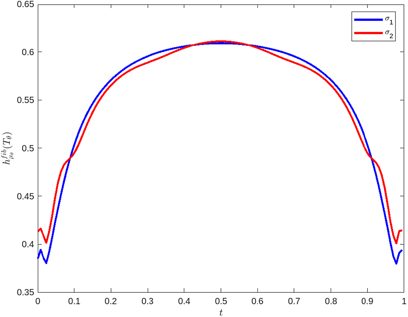
For fixed $\theta =e^{2\pi it}$ , let $T_{i}:=T_{i,\theta }, i=0,1.$ Figure 2 shows a numerical approximation of $h^{\mathrm {fib}}_{\mu _{\theta }}(\mathcal {T}_{\theta })$ over $t\in [0,1)$ for two choices of driving $\sigma _{1}, \sigma _{2}$ :

(1) $\Omega _{1}=\{0,1\}^{\mathbb {Z}}$ with $\mathbb {P}([0\cdot ])=0.2=1-\mathbb {P}([1\cdot ])$ ; here $\sigma _{1}$ is the left shift where ${\omega :=[\ldots \omega _{-1}\omega _{0}\omega _{1}\ldots ]}$ and $T_{\omega }:=T_{\omega _{0}}$ ;
(2) $\Omega _{2}=[0,1)$ and $\sigma _{2}\omega =\omega +({1}/{\pi })\text {(mod 1)}$ ; if $\omega <0.2$ , then $T_{\omega }=T_{0}$ , otherwise $T_{\omega }=T_{1}$ .

The numerical approximation of the average over $\theta \in \mathbb {T}$ is $0.5531$ for $(\mathcal {T},\sigma _{1})$ and $0.5533$ for $(\mathcal {T},\sigma _{2})$ over 10 000 steps, an error of approximately $0.10\%$ and $0.07\%$ , respectively.

Figure 2

Plot of t versus $h_{\mu _{\theta }}^{\mathrm {fib}}(\mathcal {T}_{\theta })$ , where $\theta =e^{2\pi i t}$ , for $(\mathcal {T}_{\theta },\sigma _{1})$ and $(\mathcal {T}_{\theta }, \sigma _{2})$ (color online).

A line graph comparing two curves, sigma sub 1 and sigma sub 2, plotting h super fib sub mu sub theta of T sub theta against t. See long description.

Figure 2 Long description

The x-axis is labeled t and ranges from 0 to 1 with increments of 0.1. The y-axis is labeled h super fib sub mu sub theta (T sub theta) and ranges from 0.35 to 0.65 with increments of 0.05.

Two curves are plotted:

* A blue curve representing sigma sub 1. It starts at approximately y equals 0.39 when t equals 0, dips slightly, then rises in a smooth, symmetric bell-shaped arc peaking at y equals 0.61 when t equals 0.5, before descending symmetrically to t equals 1.

* A red curve representing sigma sub 2. It follows a similar symmetric arc but exhibits small oscillations or ripples. It starts slightly higher than the blue curve at t equals 0, crosses below it around t equals 0.05, crosses above it near t equals 0.1, and stays slightly below the blue curve near the peak at t equals 0.5.

A legend in the top-right corner identifies the blue line as sigma sub 1 and the red line as sigma sub 2.

The admissibility conditions in Definition 3.1 are sufficient but not necessary for the conclusions of Theorem 1.3 and Corollary 3.5 to hold. In the following example, we give a Blaschke product cocycle which is not admissible, as Definition 3.1 $(3)$ does not hold, yet the average entropy formula still holds by direct computation.

Example 5.2. Fix $c>0.$ Let $\Omega =[0,1)$ , $\mathbb {P}=m$ and $\sigma \omega =\omega +\alpha \text { (mod 1)}$ for some fixed $\alpha \not \in \mathbb {Q}.$ For $j\in \mathbb {N}$ , let $\Omega _{j}$ be such that $\Omega =\bigcup _{j}\Omega _{j}$ and $\mathbb {P}(\Omega _{j})=({6}/({\pi ^2(j+1)^2})).$ Let $(\mathcal {T},\sigma )$ be a Blaschke product cocycle consisting of Blaschke products fixing the origin with real zeros, in particular, for each $\omega \in \Omega _{j}$ let $d_{\omega }=(j+1)^2$ , $a_{i,\omega }\in (-1,1)$ and

$$ \begin{align*}T_{\omega}(z)=\rho_{\omega} z\prod_{i=2}^{d_{\omega}}\frac{z-a_{i,\omega}}{1-a_{i,\omega}z}.\end{align*} $$ upper T Subscript omega Baseline left parenthesis z right parenthesis equals rho Subscript omega Baseline z product Underscript i equals 2 Overscript d Subscript omega Baseline Endscripts StartFraction z minus a Subscript i comma omega Baseline Over 1 minus a Subscript i comma omega Baseline z EndFraction period

upper T Subscript omega Baseline left parenthesis z right parenthesis equals rho Subscript omega Baseline z product Underscript i equals 2 Overscript d Subscript omega Baseline Endscripts StartFraction z minus a Subscript i comma omega Baseline Over 1 minus a Subscript i comma omega Baseline z EndFraction period

Furthermore, for every j such that $j^2-2j\ge c$ assume that

$$ \begin{align*}\inf_{\substack{2\le i\le (j+1)^2\\\omega\in\Omega_{j}}}|a_{i,\omega}|\ge\frac{j^2-2j-c}{j^2-2j+c}.\end{align*} $$

inf Underscript StartLayout 1st Row 2 less than or equals i less than or equals left parenthesis j plus 1 right parenthesis squared 2nd Row omega element of normal upper Omega Subscript j Baseline EndLayout Endscripts StartAbsoluteValue a Subscript i comma omega Baseline EndAbsoluteValue greater than or equals StartFraction j squared minus 2 j minus c Over j squared minus 2 j plus c EndFraction period

Then $\mathcal {T}$ is not admissible, but the conclusions of Corollary 3.5 and Theorem 1.3 hold with $\mu =m\times \mathbb {P}.$ In particular,

$$ \begin{align*}h_{\mu}(\mathcal{T})=\int_{\Omega}\int_{\mathbb{T}}\log|T_{\omega}'|\,dm\,d\mathbb{P}(\omega)+h_{\mathbb{P}}(\sigma),\end{align*} $$

but

$$ \begin{align*}\int_{\Omega}\frac{d_{\omega}}{\inf_{z\in\mathbb{T}}|T_{\omega}'(z)|}\,d\mathbb{P}(\omega)=\infty.\end{align*} $$ integral Underscript normal upper Omega Endscripts StartFraction d Subscript omega Baseline Over inf Underscript z element of double struck upper T Endscripts StartAbsoluteValue upper T prime Subscript omega Baseline left parenthesis z right parenthesis EndAbsoluteValue EndFraction d double struck upper P left parenthesis omega right parenthesis equals infinity period

Proof. First, note that each $T_{\omega }$ is expanding since

$$ \begin{align*}|T^{\prime}_{\omega}(z)|=\sum_{i=1}^{d_{\omega}}\frac{1-|a_{i,\omega}|^2}{|z-a_{i,\omega}|^2}\ge1+\sum_{i=2}^{d_{\omega}}\frac{1-|a_{i,\omega}|}{1+|a_{i,\omega}|}>1 \quad\text{for all } z\in\mathbb{T}.\end{align*} $$

StartAbsoluteValue upper T prime Subscript omega Baseline left parenthesis z right parenthesis EndAbsoluteValue equals sigma summation Underscript i equals 1 Overscript d Subscript omega Baseline Endscripts StartFraction 1 minus StartAbsoluteValue a Subscript i comma omega Baseline EndAbsoluteValue squared Over StartAbsoluteValue z minus a Subscript i comma omega Baseline EndAbsoluteValue squared EndFraction greater than or equals 1 plus sigma summation Underscript i equals 2 Overscript d Subscript omega Baseline Endscripts StartFraction 1 minus StartAbsoluteValue a Subscript i comma omega Baseline EndAbsoluteValue Over 1 plus StartAbsoluteValue a Subscript i comma omega Baseline EndAbsoluteValue EndFraction greater than 1 for all z element of double struck upper T period

For $\mathbb {P}$ -a.e. $\omega \in \Omega $ , it follows that $r_{T_{\omega }}(R)<R$ for any choice of $0<R<1$ (see Propositions 4.4, 4.5 and Corollary 4.6 [Reference González-Tokman and Peters14]). Applying Theorem 2.24, we have for $\mathbb {P}$ -a.e. $\omega \in \Omega $ ,

$$ \begin{align*}x_{\omega}=\lim_{n\to\infty}T^{(n)}_{\sigma^{-n}\omega}(z)=0\quad\text{for all } z\in D,\end{align*} $$

and $\mu _{\omega }=m.$

Then we have

$$ \begin{align*}h_{\mu}^{\mathrm{fib}}(\mathcal{T})=\int_{\Omega}\int_{\mathbb{T}}\log|T_{\omega}'|\,dm\,d\mathbb{P}(\omega),\end{align*} $$

and thus

$$ \begin{align*}h_{\mu}(\mathcal{T})=\int_{\Omega}\int_{\mathbb{T}}\log|T_{\omega}'|\,dm\,d\mathbb{P}(\omega)+h_{\mathbb{P}}(\sigma).\end{align*} $$

Note that since the zeros are real, for fixed $\omega $ and $1\le i\le d_{\omega }$ , we have $\sup _{z\in \mathbb {T}}|z-a_{i,\omega }|=1+|a_{i,\omega }|.$ From Proposition 2.3, we thus have

$$ \begin{align*} \inf_{z\in\mathbb{T}}|T_{\omega}'(z)|&=1+\inf_{z\in\mathbb{T}}\sum_{i=2}^{d_{\omega}}\frac{1-|a_{i,\omega}|^2}{|z-a_{i,\omega}|^2}\\&\le1+(d_{\omega}-1)\sup_{i=2,\ldots, d_{\omega}}\inf_{z\in\mathbb{T}}\frac{1-|a_{i,\omega}|^2}{|z-a_{i,\omega}|^2}\\&=1+(d_{\omega}-1)\sup_{i=2,\ldots, d_{\omega}}\frac{1-|a_{i,\omega}|^2}{(1+|a_{i,\omega}|)^2}\\&=1+(d_{\omega}-1)\sup_{i=2,\ldots, d_{\omega}}\frac{1-|a_{i,\omega}|}{1+|a_{i,\omega}|}\\&=1+(d_{\omega}-1)\frac{1-\inf_{i=2,\ldots, d_{\omega}}|a_{i,\omega}|}{1+\inf_{i=2,\ldots, d_{\omega}}|a_{i,\omega}|}. \end{align*} $$

StartLayout 1st Row 1st Column inf Underscript z element of double struck upper T Endscripts StartAbsoluteValue upper T prime Subscript omega Baseline left parenthesis z right parenthesis EndAbsoluteValue 2nd Column equals 1 plus inf Underscript z element of double struck upper T Endscripts sigma summation Underscript i equals 2 Overscript d Subscript omega Baseline Endscripts StartFraction 1 minus StartAbsoluteValue a Subscript i comma omega Baseline EndAbsoluteValue squared Over StartAbsoluteValue z minus a Subscript i comma omega Baseline EndAbsoluteValue squared EndFraction 2nd Row 1st Column Blank 2nd Column less than or equals 1 plus left parenthesis d Subscript omega Baseline minus 1 right parenthesis sup Underscript i equals 2 comma ellipsis comma d Subscript omega Baseline Endscripts inf Underscript z element of double struck upper T Endscripts StartFraction 1 minus StartAbsoluteValue a Subscript i comma omega Baseline EndAbsoluteValue squared Over StartAbsoluteValue z minus a Subscript i comma omega Baseline EndAbsoluteValue squared EndFraction 3rd Row 1st Column Blank 2nd Column equals 1 plus left parenthesis d Subscript omega Baseline minus 1 right parenthesis sup Underscript i equals 2 comma ellipsis comma d Subscript omega Baseline Endscripts StartFraction 1 minus StartAbsoluteValue a Subscript i comma omega Baseline EndAbsoluteValue squared Over left parenthesis 1 plus StartAbsoluteValue a Subscript i comma omega Baseline EndAbsoluteValue right parenthesis squared EndFraction 4th Row 1st Column Blank 2nd Column equals 1 plus left parenthesis d Subscript omega Baseline minus 1 right parenthesis sup Underscript i equals 2 comma ellipsis comma d Subscript omega Baseline Endscripts StartFraction 1 minus StartAbsoluteValue a Subscript i comma omega Baseline EndAbsoluteValue Over 1 plus StartAbsoluteValue a Subscript i comma omega Baseline EndAbsoluteValue EndFraction 5th Row 1st Column Blank 2nd Column equals 1 plus left parenthesis d Subscript omega Baseline minus 1 right parenthesis StartFraction 1 minus inf Underscript i equals 2 comma ellipsis comma d Subscript omega Baseline Endscripts StartAbsoluteValue a Subscript i comma omega Baseline EndAbsoluteValue Over 1 plus inf Underscript i equals 2 comma ellipsis comma d Subscript omega Baseline Endscripts StartAbsoluteValue a Subscript i comma omega Baseline EndAbsoluteValue EndFraction period EndLayout

If $c> d_{\omega }-1$ , then trivially $\inf _{z\in \mathbb {T}}|T_{\omega }'(z)|\le d_{\omega }< c+1.$ If $c\le d_{\omega }-1$ , then the hypothesis $\inf _{i=2,\ldots , d_{\omega }}|a_{i,\omega }|\le (({d_{\omega }-1-c})/({d_{\omega }-1+c}))$ gives

$$ \begin{align*}\inf_{z\in\mathbb{T}}|T_{\omega}'(z)|\le1+(d_{\omega}-1)\frac{1-\inf_{i=2,\ldots, d_{\omega}}|a_{i,\omega}|}{1+\inf_{i=2,\ldots, d_{\omega}}|a_{i,\omega}|}\le c+1.\end{align*} $$

Thus, $\mathcal {T}$ is not admissible since

$$ \begin{align*} \int_{\Omega}\frac{d_{\omega}}{\inf_{z\in\mathbb{T}}|T_{\omega}'(z)|}\,d\mathbb{P}(\omega)&\ge\frac{1}{c+1}\int_{\Omega}d_{\omega}\,d\mathbb{P}(\omega)\\&=\frac{1}{c+1}\sum_{n=1}^{\infty}n\mathbb{P}(d_{\omega}=n)\\&=\frac{1}{c+1}\sum_{j=1}^{\infty}(j+1)^2\mathbb{P}(d_{\omega}=(j+1)^2)\\&=\frac{6}{\pi^2(c+1)}\sum_{j=1}^{\infty}\frac{(j+1)^2}{j^2}=\infty. \end{align*} $$

StartLayout 1st Row 1st Column integral Underscript normal upper Omega Endscripts StartFraction d Subscript omega Baseline Over inf Underscript z element of double struck upper T Endscripts StartAbsoluteValue upper T prime Subscript omega Baseline left parenthesis z right parenthesis EndAbsoluteValue EndFraction d double struck upper P left parenthesis omega right parenthesis 2nd Column greater than or equals StartFraction 1 Over c plus 1 EndFraction integral Underscript normal upper Omega Endscripts d Subscript omega Baseline d double struck upper P left parenthesis omega right parenthesis 2nd Row 1st Column Blank 2nd Column equals StartFraction 1 Over c plus 1 EndFraction sigma summation Underscript n equals 1 Overscript infinity Endscripts n double struck upper P left parenthesis d Subscript omega Baseline equals n right parenthesis 3rd Row 1st Column Blank 2nd Column equals StartFraction 1 Over c plus 1 EndFraction sigma summation Underscript j equals 1 Overscript infinity Endscripts left parenthesis j plus 1 right parenthesis squared double struck upper P left parenthesis d Subscript omega Baseline equals left parenthesis j plus 1 right parenthesis squared right parenthesis 4th Row 1st Column Blank 2nd Column equals StartFraction 6 Over pi squared left parenthesis c plus 1 right parenthesis EndFraction sigma summation Underscript j equals 1 Overscript infinity Endscripts StartFraction left parenthesis j plus 1 right parenthesis squared Over j squared EndFraction equals infinity period EndLayout

However, the other conditions for admissibility hold from

$$ \begin{align*}1<\log\inf_{z\in\mathbb{T}}|T_{\omega}'(z)|\le \log(c+1)\end{align*} $$

and the bound on the zeros. Lastly, note that for every $\theta \in \mathbb {T}$ , the same hypotheses hold for $\mathcal {T}_{\theta }$ . Thus, $h_{\mu }(\mathcal {T}_{\theta })=h_{\mu }(\mathcal {T})$ and clearly $\bar {h}(\mathcal {T})=h_{\mu }(\mathcal {T})$ , but each $\mathcal {T}_{\theta }$ is not admissible.

Acknowledgments

The authors thank Enrique Pujals for encouraging them to pursue this project. CGT and RO acknowledge support from the Australian Research Council. CGT acknowledges Lorenzo Díaz and PUC Rio for their hospitality during a visit in 2023, where this project started. RO acknowledges the Australian Government Research Training Program for financial support.

References

Andersson, M.. Topics in Complex Analysis (Universitext). Springer-Verlag, New York, 1997.Google Scholar

Atnip, J., Froyland, G., González-Tokman, C. and Vaienti, S.. Thermodynamic formalism for random weighted covering systems. Comm. Math. Phys. 386(2) (2021), 819–902.10.1007/s00220-021-04156-1CrossRef Google Scholar

Atnip, J., Froyland, G., González-Tokman, C. and Vaienti, S.. Equilibrium states for non-transitive random open and closed dynamical systems. Ergod. Th. & Dynam. Sys. 43(10) (2023), 3193–3215.10.1017/etds.2022.68CrossRef Google Scholar

Bandtlow, O. F., Just, W. and Slipantschuk, J.. Spectral structure of transfer operators for expanding circle maps. Ann. Inst. H. Poincaré Anal. Non Linéaire 34(1) (2017), 31–43.Google Scholar

Bogenschütz, T.. Entropy, pressure, and a variational principle for random dynamical systems. Random Comput. Dynam. 1(1) (1992/93), 99–116.Google Scholar

Bogenschütz, T. and Crauel, H.. The Abramov-Rokhlin formula. Ergodic Theory and Related Topics, III (Güstrow, 1990) (Lecture Notes in Mathematics, 1514). Ed. U. Krengel, K. Richter and V. Warstat. Springer, Berlin, 1992, pp. 32–35.10.1007/BFb0097526CrossRef Google Scholar

Buzzi, J.. Exponential decay of correlations for random Lasota-Yorke maps. Comm. Math. Phys. 208(1) (1999), 25–54.10.1007/s002200050746CrossRef Google Scholar

Buzzi, J.. Absolutely continuous S.R.B. measures for random Lasota-Yorke maps. Trans. Amer. Math. Soc. 352(7) (2000), 3289–3303.10.1090/S0002-9947-00-02607-6CrossRef Google Scholar

Crovisier, S. and Pujals, E.. From zero to positive entropy. Notices Amer. Math. Soc. 69(5) (2022), 748–761.10.1090/noti2478CrossRef Google Scholar

de Faria, E. and Guarino, P.. Dynamics of Circle Mappings (IMPA Monographs), 2nd edn. Springer, Cham, 2024.10.1007/978-3-031-67495-2CrossRef Google Scholar

Dragičević, D., Hafouta, Y. and Sedro, J.. A vector-valued almost sure invariance principle for random expanding on average cocycles. J. Stat. Phys. 190(3) (2023), Paper no. 54.10.1007/s10955-023-03067-wCrossRef Google Scholar

Froyland, G., González-Tokman, C. and Murray, R.. Quenched stochastic stability for eventually expanding-on-average random interval map cocycles. Ergod. Th. & Dynam. Sys. 39(10) (2019), 2769–2792.10.1017/etds.2017.143CrossRef Google Scholar

Garcia, S. R., Mashreghi, J. and Ross, W. T.. Finite Blaschke Products and their Connections. Springer, Cham, 2018.10.1007/978-3-319-78247-8CrossRef Google Scholar

González-Tokman, C. and Peters, J.. Prevalence of stability for smooth Blaschke product cocycles fixing the origin. Discrete Contin. Dyn. Syst. 45(2) (2025), 585–606.10.3934/dcds.2024104CrossRef Google Scholar

González-Tokman, C. and Quas, A.. Stability and collapse of the Lyapunov spectrum for Perron-Frobenius operator cocycles. J. Eur. Math. Soc. (JEMS) 23(10) (2021), 3419–3457.10.4171/jems/1096CrossRef Google Scholar

Jiang, Y.. Global graph of metric entropy on expanding Blaschke products. Discrete Contin. Dyn. Syst. 41(3) (2021), 1469–1482.10.3934/dcds.2020325CrossRef Google Scholar

Khanin, K. and Kifer, Y.. Thermodynamic formalism for random transformations and statistical mechanics. Sinaiĭ’s Moscow Seminar on Dynamical Systems (American Mathematical Society Translations Series 2, 171). Ed. L. A. Bunimovich, B. M. Gurevich and Ya. B. Pesin. American Mathematical Society, Providence, RI, 1996, pp. 107–140.Google Scholar

Kifer, Y.. Equilibrium states for random expanding transformations. Random Comput. Dynam. 1(1) (1992/93), pp. 1–31.Google Scholar

Kolmogorov, A. N.. A new metric invariant of transitive dynamical systems and automorphisms of Lebesgue spaces. Trudy Mat. Inst. Steklov. 169 (1985), 94–98, 254.Google Scholar

Ledrappier, F. and Young, L.-S.. The metric entropy of diffeomorphisms. I. Characterization of measures satisfying Pesin’s entropy formula. Ann. of Math. (2) 122(3) (1985), 509–539.10.2307/1971328CrossRef Google Scholar

Ledrappier, F. and Young, L.-S.. The metric entropy of diffeomorphisms. II. Relations between entropy, exponents and dimension. Ann. of Math. (2) 122(3) (1985), 540–574.10.2307/1971329CrossRef Google Scholar

Martin, N. F. G.. On finite Blaschke products whose restrictions to the unit circle are exact endomorphisms. Bull. Lond. Math. Soc. 15(4) (1983), 343–348.10.1112/blms/15.4.343CrossRef Google Scholar

Mashreghi, J. and Fricain, E.. Blaschke Products and their Applications (Fields Institute Communications, 65). Springer and Fields Institute for Research in Mathematical Sciences, New York and Toronto, ON, 2013.10.1007/978-1-4614-5341-3CrossRef Google Scholar

Mayer, V., Skorulski, B. and Urbanski, M.. Distance Expanding Random Mappings, Thermodynamical Formalism, Gibbs Measures and Fractal Geometry (Lecture Notes in Mathematics, 2036). Springer, Heidelberg, 2011.10.1007/978-3-642-23650-1CrossRef Google Scholar

Pesin, J. B.. Characteristic Lyapunov exponents, and smooth ergodic theory. Uspehi Mat. Nauk 32(4(196)) (1977), 55–112, 287.Google Scholar

Pujals, E. R., Robert, L. and Shub, M.. Expanding maps of the circle rerevisited: positive Lyapunov exponents in a rich family. Ergod. Th. & Dynam. Sys. 26(6) (2006), 1931–1937.10.1017/S0143385706000368CrossRef Google Scholar

Ruelle, D.. An inequality for the entropy of differentiable maps. Bull. Braz. Math. Soc. (N.S.) 9(1) (1978), 83–87.10.1007/BF02584795CrossRef Google Scholar

Simmons, D. and Urbański, M.. Relative equilibrium states and dimensions of fiberwise invariant measures for random distance expanding maps. Stoch. Dyn. 14(1) (2014), 1350015 25.10.1142/S0219493713500159CrossRef Google Scholar

Sinaĭ, J.. On the concept of entropy for a dynamic system. Dokl. Akad. Nauk SSSR 124 (1959), 768–771.Google Scholar

Stein, E. M. and Shakarchi, R.. Complex Analysis (Princeton Lectures in Analysis, 2). Princeton University Press, Princeton, NJ, 2003.Google Scholar

Tischler, D.. Blaschke products and expanding maps of the circle. Proc. Amer. Math. Soc. 128(2) (2000), 621–622.10.1090/S0002-9939-99-05175-8CrossRef Google Scholar

Walters, P.. Invariant measures and equilibrium states for some mappings which expand distances. Trans. Amer. Math. Soc. 236 (1978), 121–153.10.1090/S0002-9947-1978-0466493-1CrossRef Google Scholar

Figure 1 Plot of t versus S(t)=(Q−1TQ)(t)$S(t)=(Q^{-1}TQ)(t)$, where T(z)=−((z−0.4)/(1−0.4z))2,Q(t)=e2πit$T(z)=-(({z-0.4})/({1-0.4z}))^2, Q(t)=e^{2\pi i t}$ (color online).

Figure 2 Plot of t versus hμθfib(Tθ)$h_{\mu _{\theta }}^{\mathrm {fib}}(\mathcal {T}_{\theta })$, where θ=e2πit$\theta =e^{2\pi i t}$, for (Tθ,σ1)$(\mathcal {T}_{\theta },\sigma _{1})$ and (Tθ,σ2)$(\mathcal {T}_{\theta }, \sigma _{2})$ (color online).Figure 2 long description.

Article contents

Average measure-theoretic entropy for a family of expanding on average random Blaschke products

Abstract

Keywords

MSC classification

Information

1 Introduction

Definition 1.1. (Transfer operator)

Theorem 1.3. (Average metric entropy of an admissible Blaschke product cocycle)

2 Preliminaries

2.1 Finite Blaschke products and their acims

Definition 2.1. (Inner function)

Definition 2.2. (Finite Blaschke product)

Proposition 2.3. [Reference Martin22, Proposition 1]

Theorem 2.5. [Reference Pujals, Robert and Shub26, Proposition 1.2]

Proposition 2.6. [Reference Andersson1, Proposition 1.4]

Remark 2.12. [Reference Pujals, Robert and Shub26]

2.2 Map cocycles and their measure-theoretic entropy

Definition 2.14. (Map cocycle)

Definition 2.15. ( $\mathcal {T}$ -invariant measure)

Lemma 2.16. [Reference Bogenschütz and Crauel6, Corollary 1]

Definition 2.18. (Lasota–Yorke map)

Lemma 2.19. (Duality relation)

Definition 2.20. (Variation)

Theorem 2.21. [Reference Buzzi7]

Definition 2.23. (Blaschke product cocycle)

Theorem 2.24. [Reference González-Tokman and Quas15, Theorem 1(1)]

3 Measure-theoretic entropy for an admissible Blaschke product cocycle

Definition 3.1. (Admissible Blaschke product cocycle)

Proof of Theorem 1.2(ii).

Proof of Theorem 1.2(i).

4 Average entropy over a family of admissible Blaschke product cocycles

Proof of Theorem 1.3.

5 Examples

Acknowledgments

References

Save article to Kindle

Save article to Dropbox

Save article to Google Drive

Reply to: Submit a response

Your details

You have entered the maximum number of contributors

Conflicting interests