


1. Introduction
Understanding the settling dynamics of inertial particles in turbulence is important for predicting particle transport in the atmosphere, such as aeolian transport of dust and sand (Durán, Claudin & Andreotti Reference Durán, Claudin and Andreotti2011), formation and growth of droplets and particle aggregates in clouds (Shaw Reference Shaw2003), and precipitation of hydrometeors, such as raindrops, graupels and snowflakes (Garrett et al. Reference Garrett, Yuter, Fallgatter, Shkurko, Rhodes and Endries2015; Nemes et al. Reference Nemes, Dasari, Hong, Guala and Coletti2017; Zeugin et al. Reference Zeugin, Krol, Fouxon and Holzner2020; Li et al. Reference Li, Lim, Berk, Abraham, Heisel, Guala, Coletti and Hong2021). Numerous laboratory experiments and numerical simulations have been conducted to investigate the effects of turbulence on the behaviour of inertial particles. Two evident manifestations of particle–turbulence interaction mechanisms are the formation of particle clusters and the modulation of their settling velocity (Balachandar & Eaton Reference Balachandar and Eaton2010). These phenomena are observed in certain conditions depending on the turbulence (through the Kolmogorov time scale,  $\tau _{\eta }$), and on the particle size (
 ${D_p}$), density (
 $\rho _p$) and aerodynamic properties, contributing to the definition of the particle response time,
 $\tau _p$ (Maxey & Riley Reference Maxey and Riley1983). The phenomena of clustering and enhanced settling can be described as follows: as particles preferentially concentrated in strain-dominated regions (e.g. in between vortices), they settle along the downward side of swirling motions as clusters. As a result, the fall speed of the particles on the downward side is increased. This mechanism is known as preferential sweeping (Wang & Maxey Reference Wang and Maxey1993). Studies have shown that the average settling velocity of inertial particles in turbulence can be enhanced significantly by the preferential sweeping mechanism (Wang & Maxey Reference Wang and Maxey1993; Yang & Lei Reference Yang and Lei1998; Aliseda et al. Reference Aliseda, Cartellier, Hainaux and Lasheras2002; Good et al. Reference Good, Ireland, Bewley, Bodenschatz, Collins and Warhaft2014; Falkinhoff et al. Reference Falkinhoff, Obligado, Bourgoin and Mininni2020), in particular under critical conditions, i.e. when the Stokes number
 $St = \tau _p/\tau _{\eta } \approx 1$ (Yang & Lei Reference Yang and Lei1998; Aliseda et al. Reference Aliseda, Cartellier, Hainaux and Lasheras2002; Ferrante & Elghobashi Reference Ferrante and Elghobashi2003). There are also other mechanisms that have been described to hinder the settling of inertial particles in turbulence such as loitering (Nielsen Reference Nielsen1993) and vortex trapping (Tooby, Wick & Isaacs Reference Tooby, Wick and Isaacs1977), but they usually tend to be suppressed by preferential sweeping (Good et al. Reference Good, Ireland, Bewley, Bodenschatz, Collins and Warhaft2014; Rosa et al. Reference Rosa, Parishani, Ayala and Wang2016).
Despite the large number of laboratory experiments and simulations, field measurements of inertial particles (e.g. snow particles, droplets and dust) settling in the atmospheric turbulence are scarce. The lack of field evidence is mostly due to the fact that field measurements are experimentally challenging (Shaw Reference Shaw2003): local turbulent field conditions are difficult to parameterize, and the effects of particle interaction and flow Reynolds numbers on non-Stokesian particle kinematics is far from being clear (see recent advancements by Petersen, Baker & Coletti Reference Petersen, Baker and Coletti2019; Tom & Bragg 2019; Falkinhoff et al. Reference Falkinhoff, Obligado, Bourgoin and Mininni2020). Moreover, the implementation of particle–turbulence interaction mechanisms in predictive models of settling velocity at geophysical scales is also limited, since the field conditions (e.g. wide range of turbulence scales, complex particle shape) are often different from those reproduced in laboratory experiments and simulations.
To enable spatially and temporally resolved flow measurements in the field, a super-large-scale particle image velocimetry (SLPIV), using natural snow particles as tracers, has been recently developed for studying the wake structure downstream of a utility scale wind turbine in the atmospheric boundary layer (Hong et al. Reference Hong, Toloui, Chamorro, Guala, Howard, Riley, Tucker and Sotiropoulos2014; Dasari et al. Reference Dasari, Wu, Liu and Hong2019; Abraham & Hong Reference Abraham and Hong2020) and for the study of high-Reynolds-number wall turbulence (Toloui et al. Reference Toloui, Riley, Hong, Howard, Chamorro, Guala and Tucker2014; Heisel et al. Reference Heisel, Dasari, Liu, Hong, Coletti and Guala2018). Using a similar set-up, Nemes et al. (Reference Nemes, Dasari, Hong, Guala and Coletti2017) quantified the settling trajectories of 87 000 snow particles in a 4 m (width)  $\times$ 7 m (height) field of view using particle tracking velocimetry (PTV), in parallel with a digital inline holography (DIH) system, to characterize the size and morphology of snow particles. In the absence of direct estimates of snow particle density, the acceleration probability density function (p.d.f.) obtained by PTV was used to estimate the Stokes number and the aerodynamic particle response time of snow particles (Mordant, Crawford & Bodenschatz Reference Mordant, Crawford and Bodenschatz2004; Ayyalasomayajula et al. Reference Ayyalasomayajula, Gylfason, Collins, Bodenschatz and Warhaft2006; Bec et al. Reference Bec, Biferale, Boffetta, Celani, Cencini, Lanotte, Musacchio and Toschi2006). Nemes et al. (Reference Nemes, Dasari, Hong, Guala and Coletti2017) found that the settling velocity of snow particles measured using PTV showed multifold enhancements in the atmospheric turbulence, in comparison to the still-air terminal velocity
 ${W_p}= \tau _p\cdot {g}$ predicted using the acceleration-based aerodynamic response time. Employing the same set-up, Li et al. (Reference Li, Lim, Berk, Abraham, Heisel, Guala, Coletti and Hong2021) investigated the settling and clustering of snow particles under various turbulence and snow conditions. They observed intense clustering and enhanced settling velocity during near-critical Stokes conditions, showing statistical evidence of the correlation between enhanced settling velocity and local preferential concentration, thus, indirectly supporting the preferential sweeping mechanism. Despite these major findings, both contributions could not simultaneously provide flow measurements and trajectories of snow particles.
In the present study we leverage the ability of SLPIV to measure large-scale flows and PTV to observe and track individual particles, allowing us to unveil the direct, local linkages between coherent vortex structures, snow concentration distribution and settling velocity at 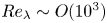 $Re_\lambda \sim O(10^3)$. We quantify here both the preferential concentration around vortices and enhanced settling velocity on the downward side of vortices, thus highlighting the fundamental mechanism of preferential sweeping. The experiment set-up, atmospheric conditions and turbulence properties are introduced in § 2. In § 3 results are presented for the quantification and visualization of the preferential sweeping mechanism. Conclusions and discussion follow in § 4.
2. Methodology
2.1. Field experiment set-up
The field deployment was conducted to acquire data on Jan. 13, 2020 between 18:00 and 21:00 local time, at the Eolos wind energy research field station in Rosemount, MN. The light sheet-based SLPIV and PTV, described in Hong et al. (Reference Hong, Toloui, Chamorro, Guala, Howard, Riley, Tucker and Sotiropoulos2014) and Nemes et al. (Reference Nemes, Dasari, Hong, Guala and Coletti2017), respectively, have been applied to capture the turbulent flow field, the trajectories and the concentration distribution of snow particles. We used a 5 kW search light with a curved mirror expanding the beam vertically into a light sheet to illuminate the snow particles. For our current measurements, the light sheet thickness is restricted to 10 cm (different from our previous measurements with 30 cm diameter light beam) at the ground and it increases to approximately 12 cm at 10 m considering the divergence angle of our search light. The light sheet was oriented to be parallel with the average wind direction and minimize the out-of-plane motion. Throughout the deployment, the instantaneous wind direction relative to the light sheet varied from  $-25^{\circ }$ to
 $15^{\circ }$. An 11-minute duration dataset has been selected for the measurement presented in this paper: within the selected period of time the wind direction was stable and well aligned with the light sheet direction with a deviation of less than
 $5^{\circ }$, and the snowfall intensity was steady, providing adequate seeding density of around 150 snow particles
 ${\textrm {m}}^{-2}$.
A Nikon D600 (Nikon Inc.) camera and a Sony A7RII (Sony Corp.) camera were equipped to record the overall flow field at 30 f.p.s. and  $1080 \times 1920\,\textrm {pixel}^2$, and the motion of snow particles at 120 f.p.s. and
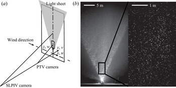
 $720\times 1280\,\textrm {pixel}^2$, respectively (referred to as SLPIV and PTV in the following sections). The start time of each recording for both cameras is documented, and a large-scale turbulent structure visible as a void at the beginning of both videos is used to further confirm the synchronization of the two datasets. Both cameras were placed on tripods with measured tilt angles from the horizontal direction (table 1). The relative locations of the two cameras and the light sheet are illustrated in figure 1(a) with the defined coordinate system (x, y, z) and corresponding velocity components (u, v, w). The specifications (e.g. duration, field of view elevation, size and distance to the camera, etc.) for the two cameras are shown in table 1.
Summary of key parameters of the SLPIV and PTV measurement set-ups for the deployment dataset used in the present paper (here FOV denotes field of view).

(a) The experiment set-up of simultaneous SLPIV and PTV measurements; (b) sample images showing the fields of view of SLPIV (left) and PTV (right).

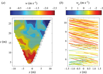
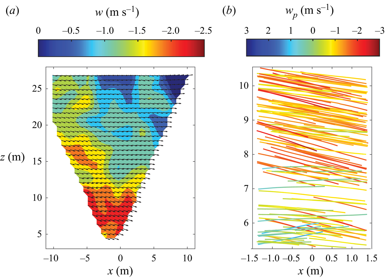
Sample images for SLPIV (Nikon camera) and PTV (Sony camera) are shown in figure 1(b), and sample results are shown in figure 2. Particle image velocimetry (PIV) analysis is conducted using LaVision Davis 8.2.0. A multi-pass setting was adopted with a final pass of 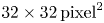 $32\times 32\,\textrm {pixel}^2$ and
 $50\,\%$ overlap. Around 700 vectors are obtained from each image pair. For PTV, we apply the learning-based tracking method from Mallery, Shao & Hong (Reference Mallery, Shao and Hong2020) using a long short-term memory network to acquire individual trajectories. Specifically, we first implement tracking methods from Crocker & Grier (Reference Crocker and Grier1996) and Ouellette, Xu & Bodenschatz (Reference Ouellette, Xu and Bodenschatz2006) to our PTV data. However, due to the lower quality of field data and relatively high particle concentration, the conventional methods generate substantially less tracks compared with those that can be determined through manual examination, potentially causing sampling bias (i.e. preferentially shorter tracks, sampling only downward tracks). Therefore, good quality trajectories generated by the conventional methods are manually selected as the training set for the learning-based method. After iterations of the training process, the well-trained model generates significantly more tracks regardless of their direction (upward or downward). In total, there are around 460 000 trajectories longer than
 $10\tau _\eta$ (where
 $\tau _\eta$ is the Kolmogorov time scale) being identified by the tracking algorithm. After the flow field and trajectories are obtained, we further identify the distribution of potential vortical structures in the flow field based on swirling strength (Zhou et al. Reference Zhou, Adrian, Balachandar and Kendall1999) and calculate the Lagrangian velocity and acceleration using the trajectory information. The swirling strength is defined as
 $\lambda _{ci}$, the imaginary part of the complex eigenvalues of the velocity gradient tensor (
 $\boldsymbol{\mathsf{D}}=\boldsymbol {\nabla }\boldsymbol {u}$). Under two-dimensional measurement,
 $\boldsymbol{\mathsf{D}}$ have either two real eigenvalues (
 $\textsf{$\mathit{\lambda}$}_\textsf{$\mathit{r}$}$) or a pair of conjugate complex eigenvalues (
 $\textsf{$\mathit{\lambda}$}_{{\mathsf{cr}}} \pm {\mathsf{i}}\textsf{$\mathit{\lambda}$}_{{\mathsf{ci}}}$), where
 $\textsf{$\mathit{\lambda}$}_{{\mathsf{cr}}}$ and
 $\textsf{$\mathit{\lambda}$}_{{\mathsf{ci}}}$ are absolute values. Thus, the vortices can be identified with finite
 $\lambda _{ci}$ (Adrian, Christensen & Liu Reference Adrian, Christensen and Liu2000). Three threshold values of the swirling strength (
 $0.4\,\text {s}^{-1}$,
 $0.5\,\text {s}^{-1}$ and
 $0.65\,\text {s}^{-1}$) are applied for detecting the vortices, and the concentration and settling velocity are analysed using all three threshold values. In the results section we will show the preferential concentration and enhanced settling with the
 $0.4\,\text {s}^{-1}$ threshold, and figures with the other thresholds will be shown in the supplementary material available at https://doi.org/10.1017/jfm.2021.816.
(a) Instantaneous flow field sample from SLPIV; (b) and snow particle trajectory samples from PTV.
Following the same procedures as in our previous studies (Hong et al. Reference Hong, Toloui, Chamorro, Guala, Howard, Riley, Tucker and Sotiropoulos2014; Toloui et al. Reference Toloui, Riley, Hong, Howard, Chamorro, Guala and Tucker2014), the traceability of snow particles for our SLPIV measurement is analysed. Specifically, the spatial resolution of the SLPIV is usually limited by the smallest interrogation window size and light sheet thickness (whichever is larger), i.e.  $l=0.66$ m in our current SLPIV measurements. Correspondingly, the flow time scale that our measurements can resolve is estimated as
 $\tau _{f} = l/u_{{rms}}=0.62$ s, where
 $u_{{rms}} = 1.07\,\textrm {m}\,\textrm {s}^{-1}$ is the root mean square (r.m.s.) of the streamwise velocity fluctuations. Thus, the particle Stokes number based on the particle response time (
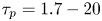 $\tau _{p} = 1.7-20$ ms, from the acceleration p.d.f. in § 3.1) and
 $\tau _{f}$ is estimated to be
 $St = \tau _{p} / \tau _{f} = 0.0028-0.032$, much smaller than the typical threshold for good traceability (i.e. 0.1 according to Tropea, Yarin & Foss Reference Tropea, Yarin and Foss2007). As a result, turbulent flows above the spatial and temporal resolution limits (i.e. 0.66 m and 0.62 s, respectively) are reasonably captured in our measurements. Note also that the mean settling velocity of the snow particles is subtracted from the SLPIV flow field.
A DIH (Nemes et al. Reference Nemes, Dasari, Hong, Guala and Coletti2017) system was deployed, and around 1580 snow particles are captured during the 11 min of the SLPIV and PTV data. The mean snow particle equivalent diameter is measured to be 0.39 mm with a standard deviation of 0.29 mm, and the average aspect ratio of the fitted minor and major ellipsoid axis is 0.62. The sample volume for the DIH measurement is  $42 \,\text {cm}^3$, thus, the mean snow particle number concentration is around
 $28\,460\,\text {m}^{-3}$, and the volume fraction is
 $3.8 \times 10^{-6}$.
2.2. Atmospheric turbulence conditions
The atmospheric and turbulence conditions during the deployment are determined using a meteorological tower instrumented with wind velocity, temperature and humidity sensors at 50 m downstream of the light sheet. Four sonic anemometers (20 Hz sampling rate, 5.8 cm horizontal measurement path length and 10 cm vertical measurement path length, CSAT3, Campbell Scientific) are installed at elevations of 10, 30, 80 and 129 m, and six cup-and-vane anemometers (1 Hz sampling rate) are installed at elevations of 7, 27, 52, 77, 102 and 126 m. Note that the measurement uncertainty of the sonic anemometer is  $\pm$0.08
 $\textrm {m}\,\textrm {s}^{-1}$ (Toloui et al. Reference Toloui, Riley, Hong, Howard, Chamorro, Guala and Tucker2014), corresponding to 1.4 % of the average wind speed. Thus, we estimate that the uncertainties for the turbulence properties would be less than 4 %. The key parameters are listed in table 2. The atmospheric stability is estimated using the bulk Richardson number
 $R_b$ and the Monin–Obukhov length
 $L_{OB}$,
 \begin{gather} R_{b}={-}|g| \Delta \overline{\theta_{v}} \Delta z /\left(\overline{\theta_{v}}\left[\left(\Delta V_{N}\right)^{2}+\left(\Delta V_{W}\right)^{2}\right]\right), \end{gather}
 \begin{gather} L_{O B}={-}U_{\tau}^{3} \overline{\theta_{v}} / \kappa g \overline{w^{\prime} \theta_{v}^{\prime}}. \end{gather}
In the equations g is the gravitational acceleration,  $\theta _{v}$ is the virtual potential temperature,
 $V_N$ and
 $V_W$ are the average wind velocity components to the North and West, respectively, measured by the sonic anemometers,
 $\kappa$ is the von Kármán constant and
 $U_{\tau }$ is the shear velocity estimated from the Reynolds stresses (Stull Reference Stull1988), where
 $U_{\tau }=(\langle V_N^{\prime } V_Z^{\prime }\rangle ^{2}+\langle V_W^{\prime } V_Z^{\prime }\rangle ^{2})^{1/4}$. The average velocity differences are calculated from the sonic anemometers at the top (129 m) and bottom (10 m) which yields a height difference
 $\Delta z$ of 119 m. The Monin–Obukhov length and all other turbulence conditions are measured with the data from the 20 Hz sonic sensor at 10 m. For the duration of the analysed dataset, the bulk Richardson number and the Monin–Obukhov length indicate that the atmospheric boundary layer during the experiment is near-neutrally stratified (typically for the near-neutrally stratified atmospheric boundary layer,
 $R_b$ ranges from 0 to 0.25 and the stability parameter (
 $z/L_{OB}$) ranges from 0 to 0.1 as suggested by Stull Reference Stull1988 and Högström, Hunt & Smedman Reference Högström, Hunt and Smedman2002).
Estimated meteorological and turbulence conditions from the sonic anemometer at  $z = 10\,\text {m}$. See the text for the definition of the symbols.

The turbulence conditions are estimated using the methods described in Nemes et al. (Reference Nemes, Dasari, Hong, Guala and Coletti2017) and Li et al. (Reference Li, Lim, Berk, Abraham, Heisel, Guala, Coletti and Hong2021). Velocity data from the sonic anemometer at 10 m are used for the flow characterization, consistent with the sample area elevation ranges of the SLPIV (from 3 m to around 40 m) and PTV (from 5.3 m to 10.6 m) measurements.The integral time scale  $\tau _{L}$ and the length scale L are estimated based on the temporal autocorrelation function
 $\rho _{u u}$,
 \begin{gather} \rho_{u u}(\tau)=\left\langle u^{\prime}(t) u^{\prime}(t+\tau)\right\rangle / u^{\prime 2}, \end{gather}
 \begin{gather} \tau_{L}=\int_{0}^{T_{0}} \rho_{u u}(\tau)\,\textrm{d} \tau, \end{gather}
 \begin{gather} L=u_{rms} \tau_{L}. \end{gather}
In these equations t is the variable time,  $\tau$ is the time difference and
 $T_0$ is the first zero-crossing point of the auto-correlation function. The turbulence dissipation rate
 $\epsilon$ is estimated using the second-order structure function of the streamwise velocity component, applying the Taylor hypothesis to convert the measured time series into spatial velocity variations,
 \begin{gather} D_{11}(\tau)=\langle[u^{\prime}(t+\tau)-u^{\prime}(t)]^{2}\rangle, \end{gather}
 \begin{gather} D_{11}(r)=C_{2} \epsilon^{2 / 3} r^{2 / 3}. \end{gather}
With the Kolmogorov prediction for the second-order structure function in the inertial range (2.7), where  $C_2$ is a constant of around 2 in high-Reynolds-number turbulence (Saddoughi & Veeravalli Reference Saddoughi and Veeravalli1994), we can estimate the turbulence dissipation rate
 $\epsilon =(D_{11} /(C_{2} r^{2 / 3}))^{3 / 2}$. Furthermore, we calculated the Kolmogorov time and length scale,
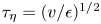 $\tau _{\eta }=(v / \epsilon )^{1 / 2}$ and
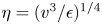 $\eta =(v^{3} / \epsilon )^{1 / 4}$, the Taylor microscale
 $\lambda =u_{rms}(15 v / \epsilon )^{1 / 2}$ and the Reynolds number
 $Re_{\lambda }=u_{{rms}} \lambda / \nu$, where
 $\nu$ is the kinematic viscosity of air and
 $u_{{rms}}$ is the r.m.s. of the velocity fluctuations
 $u^{\prime }$.
3. Results
3.1. Snow particle acceleration and Stokes number
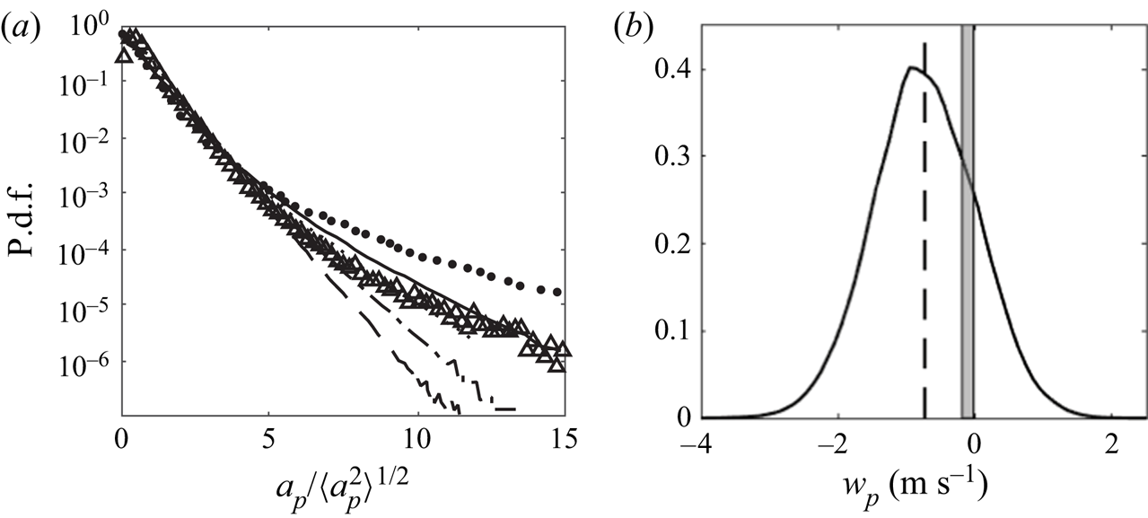
The snow particle acceleration and vertical velocity obtained from PTV analysis are evaluated in this section. Figure 3(a) shows the p.d.f. of the fluctuations of the snow particle acceleration normalized by their r.m.s. value. The p.d.f. is compared with data from previous laboratory experiments and numerical simulations of tracers and inertial particles in isotropic turbulence (Mordant et al. Reference Mordant, Crawford and Bodenschatz2004; Ayyalasomayajula et al. Reference Ayyalasomayajula, Gylfason, Collins, Bodenschatz and Warhaft2006; Bec et al. Reference Bec, Biferale, Boffetta, Celani, Cencini, Lanotte, Musacchio and Toschi2006). In figure 3(a) the exponential tail of the in-plane acceleration p.d.f. curve of snow particles lies in between the curves with Stokes numbers of 0.16 and 1.01 from Bec et al. (Reference Bec, Biferale, Boffetta, Celani, Cencini, Lanotte, Musacchio and Toschi2006), while a comparison of streamwise acceleration with Ayyalasomayajula et al. (Reference Ayyalasomayajula, Gylfason, Collins, Bodenschatz and Warhaft2006), in a similar boundary layer flow, seem to narrow the range to 0.09–0.15. As discussed in Nemes et al. (Reference Nemes, Dasari, Hong, Guala and Coletti2017), the acceleration kurtosis manifests the tendency of inertial particles to experience only a portion of the high acceleration events sustained by fluid parcels. The direct numerical simulation by Ireland, Bragg & Collins (Reference Ireland, Bragg and Collins2016) showed that the kurtosis of acceleration becomes insensitive to the change of Reynolds number with  $St > 0.1$ and
 $Re_{\lambda } > 398$ (e.g. as
 $Re_{\lambda }$ changes from 398 to 597 at
 $St = 0.1$, the kurtosis of acceleration increases only 3 %, and the change becomes smaller at higher
 $St$). Therefore, following the reasoning in our previous studies (Nemes et al. Reference Nemes, Dasari, Hong, Guala and Coletti2017; Li et al. Reference Li, Lim, Berk, Abraham, Heisel, Guala, Coletti and Hong2021), we extend the comparison of the acceleration p.d.f.s to the atmospheric turbulence case with high
 $Re_{\lambda }$ investigated here, and conservatively estimate the Stokes number in the range of 0.09–1.01.
(a) Probability density functions of in-plane snow particle acceleration from PTV (triangles), compared with  $St$ = 0 from Mordant et al. (Reference Mordant, Crawford and Bodenschatz2004) (dots), and Bec et al. (Reference Bec, Biferale, Boffetta, Celani, Cencini, Lanotte, Musacchio and Toschi2006) (
 $St$ = 0.16, solid line;
 $St$ = 0.37, dotted line;
 $St$ = 1.01, dash–dotted line;
 $St$ = 2.03, dashed line); (b) comparison of the measured distribution (solid line) and average (dashed line) of settling velocity with the estimated range of still-air terminal velocities (grey region).

With the estimated  $St$, the aerodynamic particle response time of the observed snow particles is predicted to be in the range of 1.7 ms to 19.6 ms, where
 $\tau _p = St\cdot \tau _{\eta }$, leading to a still-air terminal velocity defined by
 $W_p= \tau _p\cdot {g}$ and estimated between 0.02
 $\textrm {m}\,\textrm {s}^{-1}$ and 0.19
 $\textrm {m}\,\textrm {s}^{-1}$. The estimated Stokes number indicates a near-critical condition (
 $St\sim \textit {O}(1)$), anticipating the occurrence of preferential concentration (clustering) and sweeping, as well as enhanced settling velocity. In figure 3(b) we compare the vertical velocity distribution (solid line) from PTV (the average vertical velocity (
 $\langle w_p\rangle$) of 0.73
 $\textrm {m}\,\textrm {s}^{-1}$ is indicated as a dashed line) with the estimated terminal velocity range accounting for the uncertainty in the Stokes number (grey region). The increase is evident and multifold (around seven times larger on average,
 $\langle w_p\rangle / \overline {W}_{p}$). This enhancement is consistent with what has been observed in the previous study by Nemes et al. (Reference Nemes, Dasari, Hong, Guala and Coletti2017) (around three times enhancement on average). However, since our estimated range for
 $St$ is closer to the critical value, the observed enhancement here is higher.
Note that the corresponding particle Reynolds number  $Re = {\langle w_p\rangle }D/\nu$ based on the measured settling velocity and particle size is
 $\sim$16.8, implying that a non-Stokesian drag correction is required. Due to the disk-like shape of the observed snow particles, the Schiller–Neumann approach based on the Reynolds-corrected sphere drag is not recommended, which in part justifies the estimation of the Stokes number from the acceleration p.d.f. with no explicit dependency on density, and size. The only option to account for snow morphology is to use the semi-empirical
 $\chi$ number approach proposed by Böhm (Reference Böhm1989), corrected by Heymsfield & Westbrook (Reference Heymsfield and Westbrook2010), and also employed in Nemes et al. (Reference Nemes, Dasari, Hong, Guala and Coletti2017). The resulting parameterization leads to
 $\chi = 997$ and a drag coefficient of
 $C_{D}=3.53$, which is not unusual given the relatively low particle Reynolds number (Westbrook & Sephton Reference Westbrook and Sephton2017). It is important to stress that the
 $\chi$ number accounts for the snow morphology effects on drag (Garrett et al. Reference Garrett, Yuter, Fallgatter, Shkurko, Rhodes and Endries2015; Dunnavan et al. Reference Dunnavan, Jiang, Harrington, Verlinde, Fitch and Garrett2019), not necessarily for the effect of ambient turbulence, which is the main point of this work.
3.2. Preferential distribution of snow particle concentration
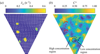
Snow particle concentration around vortices in the flow is first evaluated using the SLPIV data. As shown in an instantaneous flow sample (figure 4a), the vortices are identified using the swirling strength derived from the velocity fields of SLPIV as described in detail in § 2.1. Subsequently, the particle number concentration within and around the vortices is estimated using the image intensity ( $I(x,z,t)$) of the SLPIV data. The estimation of concentration using image intensity is supported by Raffel et al. (Reference Raffel, Willert, Scarano, Kähler, Wereley and Kompenhans2018) which shows that the image intensity of PIV is proportional to the concentration of particles with the same averaged diameters. However, factors such as stochastic light attenuation by particles within the light sheet and in between the light sheet and the cameras, as well as the power fluctuation of the search light might lead to a nonlinear relationship between the light intensity and local particle concentration (Kalt, Birzer & Nathan Reference Kalt, Birzer and Nathan2007; Banko et al. Reference Banko, Villafañe, Kim, Esmaily and Eaton2019). Nevertheless, due to relatively low volume fraction, the light attenuation by particles between the light sheet and the cameras is not inferred to be dominant as compared with the other two factors. Furthermore, to minimize the spatial and temporal non-uniformity in background image intensity due to the decay of light intensity with height and its fluctuation over time, relative concentration
 $C^{*}=I(x, z, t) / I(x, z)_{{10s,avg}}$ is defined according to Li et al. (Reference Li, Lim, Berk, Abraham, Heisel, Guala, Coletti and Hong2021), where
 $I(x, z)_{{10s,avg}}$ is an average of the intensity of images recorded in a 10 s moving window. Figure 4(b) shows the relative concentration of the flow sample corresponding to figure 4(a). In particular, we observe that snow concentration is low within the vortex cores. The phenomenon is considered to be a result of the inertia bias (Maxey Reference Maxey1987), i.e. inertial particle trajectories are biased towards the region of low vorticity. Remarkably, for all three strong vortices (i.e. vortices with high swirling strength values) highlighted in the figure, including both prograde and retrograde vortices, the particle concentration is preferentially higher on the downward flow side of the vortices (referred to as preferential concentration hereafter).
(a) Swirling strength contour of an instantaneous sample (threshold  $0.4\,\text {s}^{-1}$ applied) with relative flow velocity vectors (white arrows, subtracted by the convective velocity of
 $3.4\,\textrm {m}\,\textrm {s}^{-1}$ of the prograde vortex at the centre left of the field of view). (b) Corresponding snow particle concentration colourmap (
 $C^{*}$ is the relative concentration) with vortices detected from (a). Note that the white dashed lines represent vortex boundaries, red arrows indicate prograde vortices and the blue arrow indicates the retrograde vortex, the black circle and arrow define the coordinate system of the local vortex.

It is worth noting that the relative concentration map in figure 4(b) seems to suggest the clustering of snow particles in the atmospheric surface layer similar to those studied in our previous work (Li et al. Reference Li, Lim, Berk, Abraham, Heisel, Guala, Coletti and Hong2021). However, the clusters in figure 4(b) are on smaller scales and do not exhibit a clear preferential orientation in comparison to those presented in Li et al. (Reference Li, Lim, Berk, Abraham, Heisel, Guala, Coletti and Hong2021) with the January 2019 dataset. The difference is mainly caused by relatively lower turbulence and snow concentration in the current cases which lead to a weaker interaction between particles and turbulence. In addition, since the current study focuses on elucidating the connection between the vortical structures in the turbulent flow and settling of individual snow particle, the PTV was designed to have a more focused field of view (3 m  $\times$ 5 m, smaller than the integral scale), limiting our ability to quantify the large-scale clusters that extend beyond our region of interest.
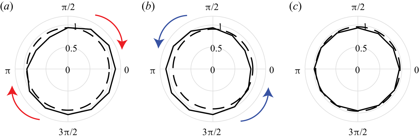
To substantiate the observation of preferential concentration associated with the presence of vortices in the flow, the ensemble-averaged concentration contours are calculated for prograde (28 700 prograde vortices identified) and retrograde vortices (9,700 retrograde vortices), respectively. As shown in figure 5, the averaged concentration is determined for both the central region defined as the region within half of the effective radius (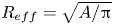 $R_{{eff}}=\sqrt {A / {\rm \pi}}$, where A is the area of the vortex region detected through the swirling strength criterion) from the centre of the vortex, and in the rest of proximity, defined as the region from
 $0.7R_{{eff}}$ to
 $1.4R_{{eff}}$ from the centre. The latter is divided into twelve angular sectors with angle of
 ${\rm \pi} / 6$. For both prograde (figure 5a) and retrograde vortices (figure 5b), it is observed that the particle concentration is higher on the downward side, than that on the upward side and in the centre of vortices. For reference, the averaged concentration distribution in the background (figure 5c) does not exhibit any appreciable preferential concentration. For each prograde/retrograde vortex, the reference background is defined as a circular region that has a radius equal to the
 $R_{{eff}}$ of the prograde/retrograde vortex with a centre at a randomly selected location in the SLPIV measurement field of view. In addition, the averaged particle concentration is relatively higher at the bottom of the downward side for retrograde vortices, possibly due to gravity and downward fluid motion causing a stronger preferential concentration effect. But for prograde vortices, relative concentration is more uniformly distributed on the downward side. Such a discrepancy can be explained by the different organizations of prograde and retrograde vortices in the atmospheric surface layer. Specifically, the prograde vortices tend to form in packets (Christensen & Adrian Reference Christensen and Adrian2001), predominantly located in the internal shear layers in the atmospheric surface layer, the interaction between snow particles around a certain prograde vortex with adjacent vortices may smooth out the particle concentration on the downward side.
Comparison between the ensemble-averaged concentration from the SLPIV dataset in the central region (dashed lines), defined as the region within half  $R_{{eff}}$ from the vortex centre where
 $R_{{eff}}$ is the effective radius of the vortices, and in the proximity (solid lines), defined as the region from
 $0.7R_{{eff}}$ to
 $1.4R_{{eff}}$ from the centre spanning a circumferential angle range of
 ${\rm \pi} / 6$, for (a) prograde vortices, (b) retrograde vortices and (c) reference background. For each prograde/retrograde vortex, the reference background is defined as a circular region that has a radius equal to the
 $R_{{eff}}$ of the prograde/retrograde vortex with a centre at a randomly selected location in the SLPIV measurement field of view.

It is well known that preferential concentration in turbulent flows is a multi-scale phenomenon. As shown in (Baker et al. Reference Baker, Frankel, Mani and Coletti2017), particles start clustering at the Kolmogorov scale when they preferentially sample the high strain regions in the flow. As the clusters yield a larger response time than that of individual particles, they can subsequently interact with larger-scale flow structures and grow in size up to the integral scale (see examples in Li et al. Reference Li, Lim, Berk, Abraham, Heisel, Guala, Coletti and Hong2021). However, due to the limit of the SLPIV resolution, we can only resolve vortices above a certain size ( $\sim$66 cm) in our measurements. Therefore, the preferential concentration statistics shown in figure 5 are captured only by sampling large, energetic vortices leaving a signature several times larger than the Taylor microscale in our coarsely resolved turbulent flow. Nevertheless, the estimated Stokes number in § 3.1 (with the upper range close to the critical condition) suggests strong interaction between the particles and flow structure at the Kolmogorov scales, causing preferential concentration and clustering that cannot be resolved with the current SLPIV measurement. We thus acknowledge resolving a limited range of scale contributing to particle clustering, but capturing the key mechanism governing preferential sweeping at the resolved scale.
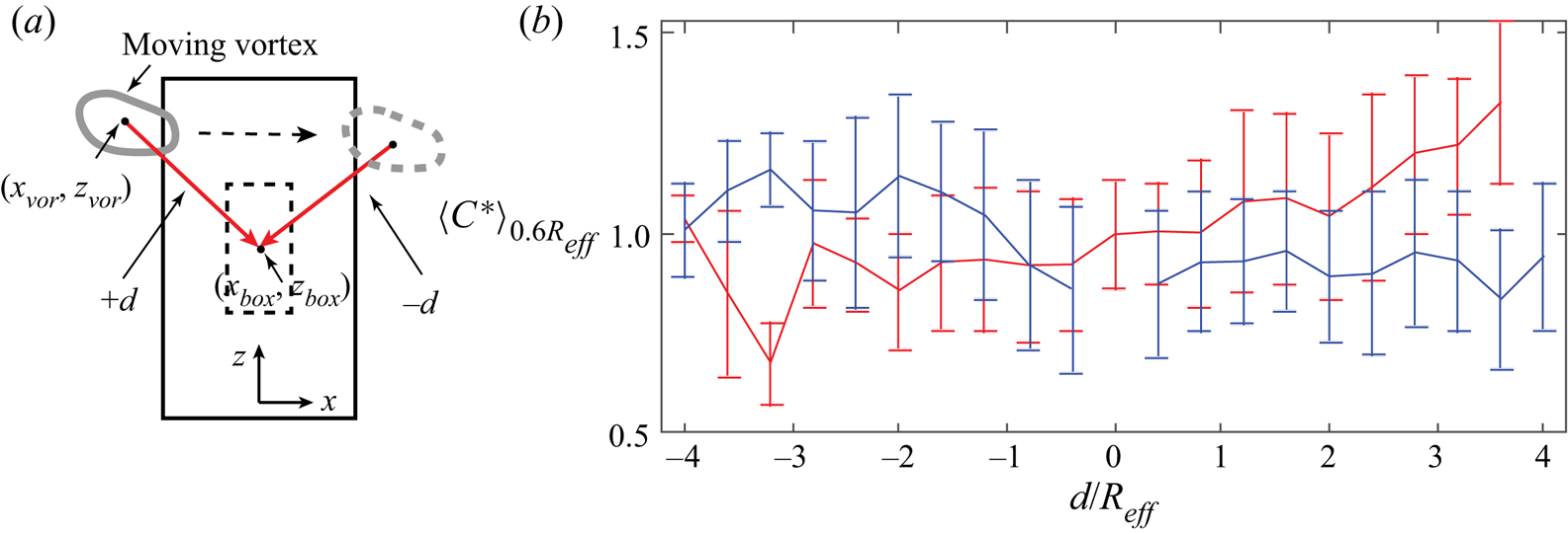
Furthermore, we examine the images from the PTV measurements in which individual snow particles can be counted and tracked within and around the vortices (see movies 1 and 2 in the supplementary material), supporting the observation of preferential concentration based on the change in the intensity of images from SLPIV. We first select the vortices determined from the corresponding SLPIV measurements at the same time instant as the PTV with overlapping field of view. Most of these vortices have an equivalent diameter  $\gtrsim$1.3 m and are only partially inside the PTV images as they move across the small (relative to SLPIV) sample area of PTV. As a result, the previous method (that for SLPIV) for estimating particle concentration cannot be applied. Instead, as illustrated in figure 6(a), a box counting method is used to determine the change of snow particle concentration due to the presence of vortices in the PTV sample area (note that the uncertainty of particle concentration associated with the changing light sheet thickness within the PTV field is estimated to be less than 9 %). A fixed counting box (
 $100\times 200\,\text {pixel}^2$) is selected at the centre of the PTV area. When the vortex appears in the sample area of PTV, the total number of snow particles in the box is counted. The relative displacement (d) between the vortex centre (
 $x_{{vor}}$,
 $z_{{vor}}$) and box centre (
 $x_{{box}}$,
 $z_{{box}}$) is calculated as
 \begin{equation} d=\frac{x_{{box}}-x_{{vor}}}{\left|x_{{box}}-x_{{vor}}\right|} \sqrt{\left(x_{{box}}-x_{{vor}}\right)^{2}+\left(z_{{box}}-z_{{vor}}\right)^{2}}. \end{equation}
Particularly, the sign of the relative displacement indicates which side the particles are located with respect to the moving vortex. Similar to that in the SLPIV data processing, to account for the variation of snow particle concentration in the background, the relative concentration for PTV data ( $C^{*}$) is estimated using total particle number counts in the box at each time instant divided by the averaged total particle counts for the time duration during which each vortex is present in the sample area of PTV. Subsequently, the ensemble averaged
 $C^{*}$ in a bin of a width of
 $0.6R_{{eff}}$ (
 $\langle C^{*}\rangle _{0.6 R_{{eff}}}$) at different relative displacements is determined for prograde (550 in total) and retrograde (380 in total) vortices, respectively (figure 6b). As the figure shows, for prograde vortices, the
 $\langle C^{*}\rangle _{0.6 R_{{eff}}}$ is evidently higher on the downward side of the vortices (positive
 $d$). For retrograde vortices, the
 $\langle C^{*}\rangle _{0.6 R_{{eff}}}$ also yields larger values on the downward side (negative
 $d$), though the difference in
 $\langle C^{*}\rangle _{0.6 R_{{eff}}}$ between two sides appears to be smaller than that observed for prograde vortices. To determine the significance of the difference in
 $\langle C^{*}\rangle _{0.6 R_{{eff}}}$, we conduct a t-test to the concentration distribution at the two sides of the vortices: the particle concentration on the downward side is in general 13 %–22 % higher (at 95 % confidence level) than that at the upward side for both prograde and retrograde vortices. These trends (see also the supplementary material) provide further support of the preferential concentration. Nevertheless, due to the limited number of vortices that can be simultaneously detected by SLPIV and PTV, the standard deviation of the
 $\langle C^{*}\rangle _{0.6 R_{{eff}}}$ presented in the current analysis is considerable. In addition, we would like to point out that the statistical signature of preferential concentration observed in PTV is likely to be underestimated potentially due to the relatively large counting box size used in the analysis in comparison to the size of vortices.
(a) A schematic showing the box counting process to determine the change of snow particle concentration due to the presence of a vortex (grey solid and dashed contours) in the PTV sample area (black solid line). The vortex is determined from the corresponding SLPIV measurement at the same time instant as the PTV. A fixed counting box (black dashed line,  $100 \times 200\, \text {pixel}^2$) is selected at the centre of the PTV area. The relative displacement (red arrow) between the vortex centre (
 $x_{{vor}}$,
 $z_{{vor}}$) and box centre (
 $x_{{box}}$,
 $z_{{box}}$) is defined by (3.1). (b) The ensemble-averaged particle concentration (
 $\langle C^{*}\rangle _{0.6 R_{{eff}}}$) at different relative displacements with respect to the vortex centre. In total, 550 prograde (red line) and 380 retrograde (blue line) vortices are selected for the ensemble average, respectively. The bin of relative displacement (
 $\Delta d$) used in ensemble average has a width of
 $0.6R_{{eff}}$ and spaced
 $0.4R_{{eff}}$ from adjacent bins (
 $\sim$33 % overlap). The bin size and spacing are determined to ensure sufficient statistical convergence of the data.

3.3. Enhanced settling velocity due to preferential sweeping
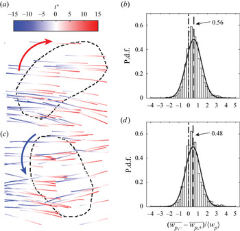
In this subsection we investigate how the settling velocity of snow particles is influenced by the presence of the vortical structures in the flow. Consistent with the method presented in the last section, the vortices are first identified using SLPIV data. Subsequently, the particle trajectories around these identified vortices are extracted from PTV for the following analysis. For the prograde vortex (figure 7a), the settling velocity of particles increases when moving toward the downward side (right-hand side in the sample) of the vortex. Similarly, for the retrograde vortex (figure 7c), the settling of snow particles slows down; some particles are even lifted upward, as they travel to the upward side (right-hand side in the sample) of the vortex. Both cases illustrate clearly higher settling velocities of the snow particles situating on the downward side of the vortices.
(a,c) Samples of snow particle trajectories around a prograde vortex (a) and a retrograde vortex (c) (see also movies 1 and 2 uploaded in the supplementary material). Black dashed lines represent vortex boundaries, and trajectories are coloured based on the dimensionless time  $t^{*}$, defined as the difference between the timestamps of snow particles and that of a selected vortex at one time instant normalized by the Kolmogorov time scale. (b,d) Histograms of the differences between the settling velocities on the downward sides and upward sides for (b) prograde and (d) retrograde vortices (a total of 4300 prograde and 1700 retrograde vortices are identified), normalized by the average vertical velocity
 $\langle w_{p}\rangle$ of snow particles tracked with zeros marked by the dash–dotted lines, and the dashed lines represent the average velocity difference in each case. The bin size is chosen to be one fifth of
 $\langle w_{p}\rangle$. The histograms are compared with the Gaussian distributions marked by the solid lines.

To further substantiate these observations, the average vertical accelerations conditioned on the downward ( $\overline {a_{p,-}}$) and the upward (
 $\overline {a_{p,+}}$) sides of prograde and retrograde vortices are calculated, and the histograms of settling velocity difference between the downward (
 $\overline {w_{p,-}}$) and upward (
 $\overline {w_{p,+}}$) sides of vortices, i.e.
 $\overline {w_{p,-}}-\overline {w_{p,+}}$, normalized by the ensemble average snow particle vertical velocity (
 $\langle w_{p}\rangle =0.73 \,\mathrm {m} \, \mathrm {s}^{-1}$) are presented for all prograde (figure 7b) and retrograde (figure 7d) vortices, respectively. The
 $\overline {a_{p,-}}$,
 $\overline {a_{p,+}}$,
 $\overline {w_{p,-}}$ and
 $\overline {w_{p,+}}$ are calculated by averaging the vertical velocities of particles within boxes ranging from
 $0.5R_{{eff}}$ to
 $1.5R_{{eff}}$ to the centre of vortices in the x direction and covering the whole diameter (
 $2R_{{eff}}$) in the vertical direction at the two sides of the vortices. Specifically, for prograde vortices, the two conditionally averaged accelerations are
 $\overline {a_{p,-}} = -0.16 \pm 2.20\, \textrm {m}\,\textrm {s}^{-2}$ on the downward side and
 $\overline {a_{p,+}} = 0.0065 \pm 2.54\, \textrm {m}\,\textrm {s}^{-2}$ on the upward side. While for retrograde vortices,
 $\overline {a_{p,-}} = -0.33 \pm 2.93\,\textrm {m}\,\textrm {s}^{-2}$ and
 $\overline {a_{p,+}} = 0.12 \pm 2.09\,\textrm {m}\,\textrm {s}^{-2}$. These conditional averages support the fact that particles on the downward side of vortices would accelerate with the flow and particles falling on the upward side would decelerate, or even be lifted up. Note that the variability in acceleration (e.g. the standard deviation) is much higher than that for the settling velocity due to the higher-order derivative in the acceleration calculation. Moreover, the settling velocity differences display a near Gaussian distribution with the mean value above zero. As compared with Gaussian distribution with the same mean value and standard deviation, the p.d.f.s of settling velocity difference exhibit higher probability near the mean values and heavier tails on the right-hand side for both prograde and retrograde vortices, indicating statistically higher settling velocities on the downward side of vortices. Specifically, approximately 78 % of the prograde vortices yield a higher settling velocity on the downward side with an average settling velocity differences of 0.56
 $\langle w_p\rangle$, and the proportion is approximately 73 % for the retrograde vortices with an average settling velocity difference of 0.48
 $\langle w_p\rangle$. Note that the total number of vortices identified in figure 7 is larger than that for particle concentration in figure 6. It is because we identify an individual vortex from the PTV field for settling velocity analysis, while vortices selected for preferential concentration in figure 6 are tracked across the region of interest.
However, not every single occasion is observed with higher settling velocity at the downward side of vortices, due to the fact that the vortices detected in the current study are planar projections of highly complex three-dimensional vortices. In addition, the snow particles interacting with one vortex can also be affected by adjacent vortices in the atmosphere, which are usually weaker and less appreciable in the SLPIV data as compared with the vortices analysed. Nevertheless, we observe an increasing percentage of events showing such a trend when we sample vortices with higher swirling strength and the percentage for prograde vortices is consistently higher than that for retrograde vortices. Such discrepancies are likely due to the difference in self-organization characteristics for prograde and retrograde vortices (i.e. prograde vortices are found to be predominantly located in the proximity of internal shear layers as shown in the field PIV measurement in the atmospheric surface layer by Heisel et al. Reference Heisel, Dasari, Liu, Hong, Coletti and Guala2018). Therefore, prograde vortices could have a cumulative and stronger effect on the enhanced settling of nearby snow particles compared with retrograde vortices. Nevertheless, with the observed preferential concentration from § 3.2 and statistically higher settling velocity on the downward side of the vortices, we conclude that under near-critical conditions ( $St\sim O(1)$) observed in our field measurements, preferential sweeping plays a significant role in controlling the settling velocity of hydrometeors in the atmospheric turbulence.
4. Conclusions and discussion
In this paper we present the first field study of snow settling dynamics based on simultaneous measurements of the atmospheric flow field using a SLPIV and snow particle trajectories using PTV within the SLPIV sample area. Our results reveal the direct linkage among the coherent vortex structures in the atmospheric turbulence, and the concentration distribution and settling dynamics of snow particles in the field. Specifically, we observe a settling velocity enhancement of around seven folds on average compared with the estimated still-air terminal velocity. This value is larger than what has been observed in our previous field study (Nemes et al. Reference Nemes, Dasari, Hong, Guala and Coletti2017), potentially due to the fact that the Stokes number associated with the snow particles in the present deployment is closer to the critical condition ( $St\sim O(1)$). Using the SLPIV we are able to detect the strong vortices present in the atmospheric turbulent flow, and we show that the snow concentration (represented by the variation in the particle image intensity in SLPIV) is preferentially higher on the downward side for both prograde and retrograde vortices in the flow. This observation is further substantiated by counting individual snow particles around the vortices using PTV data. The result indicates an average of 18 % higher concentration on the downward side of the detected strong vortices present in our study. In addition, the samples of snow particle trajectories around vortices from PTV demonstrate that snow particles accelerate as they move toward the downward side of vortices and decelerate or even are lifted upward when travelling to the upward side. Based on the histograms of snow settling velocity from PTV, we show that the snow particles on the downward side of vortices yield a statistically higher settling velocity than that at the upward side, with an average difference of approximately 52 % of the mean settling velocity.
Our results provide direct evidence and underlying mechanisms for the preferential concentration and preferential sweeping during snow particles settling in the atmospheric surface layer. While the presented results focus on the quantification of particle–turbulence interaction mechanisms at the scale of individual vortices, we recognize that atmospheric turbulence in the near-neutrally stratified boundary layer in our study contains vortices over a broad range of scales and intensities. Therefore, we hypothesize that the preferential paths of highly concentrated particles along layers of vortices are likely to produce a cumulative effect on enhancing the settling of the snow particles. This conceptual framework has not been considered in current snow settling models. Under this framework, our observed results of preferential concentration and preferential sweeping may be critical to inform a stochastic model to reproduce the observed fall speed under specific micrometeorological conditions. By incorporating the framework, it may be possible to model the settling of snow particles starting from the still-air terminal velocity with specific drag coefficient and sampling a population of vortices consistent with the inertial range in the air column. Under the assumption of accelerated preferential paths, each snow particle has a large probability to sample a number of vortices, and the effects of both the drag force and vortex flow sweeping will progressively enhance the settling velocity to a certain value. With this perspective, it is reasonable to hypothesize that the multifold increase in observed settling velocity compared with the still-air terminal velocity, as well as its large variability, is a result of the cumulative effect of particles settling through the turbulent air column occupied by many vortices. In addition, the disparity in settling velocities observed on the downward and upward sides of vortices of  $0.4\,\textrm {m}\,\textrm {s}^{-1}$ might also be directly affected by the azimuthal velocity of the flow around vortices, manifested in vertical velocity fluctuations that are more readily available from the measured flow field.
In the end, we acknowledge the uncertainties involved in our concentration measurement using box counting from the PTV data. Such uncertainties are largely caused by the limited data of synchronized SLPIV and PTV measurements from our field deployment. Nevertheless, the main observations related to the snow particle concentration and settling dynamics present in our study are still statistically significant. A second relevant uncertainty is in the estimate of the snow particle velocity in still air. While the Stokes number range is conservatively defined, it would still be important to provide a direct estimate of the snow particle density, combining measurements of single particle volume with the weighing of particle ensemble in time. We expect that more converged trends can be obtained with an increasing number of deployments. In particular, we expect to extend our current field PTV to a three-dimensional imaging system using multiple cameras. Such an upgraded system will allow us to quantify, more accurately, the particle concentration and distribution, particle setting kinematics (e.g. curvature of the trajectories) and dynamics (e.g. acceleration, inertial response) associated with the presence of three-dimensional vortex structures in the atmospheric turbulence.
Supplementary movies
Supplementary movies are available at https://doi.org/10.1017/jfm.2021.816.
Acknowledgements
The authors thank engineers from St Anthony Falls Laboratory, including J. Tucker, J. Mullin, C. Ellis, J. Marr, C. Milliren and D. Christopher, for their assistance in the experiments.
Funding
This work is supported by the National Science Foundation (Program Manager, Nicholas Anderson) under grant NSF-AGS-1822192.
Declaration of interests
The authors report no conflict of interest.