

1. Introduction
To predict accurately the transition from laminar flow to turbulence in high-speed boundary layers is a crucial issue in aircraft designs because the surface drag and heat flux differ markedly in laminar and turbulent phases. In practical applications, idealised (smooth and isothermal) walls are rarely seen, and surface inhomogeneity, such as roughness, appears frequently. For a hypersonic flight under cruise conditions, different parts of the flight surface may show different temperatures due to the diverse thermal conductivity of their materials, leading to the appearance of an array of heating or cooling sources. Moreover, surface ablation may also appear due to the strong aerodynamic heating, which could enhance the intensity of a heating or cooling source (HCS). Another motivation of the present study is from the viewpoint of the laminar flow control. In order to reduce the total friction and heat flux, to maintain the laminar phase longer or to delay the transition onset is favourable. An HCS may be a potentially efficient strategy for the laminar flow control, and a systematic study of its impact on transition is needed.
The laminar–turbulent transition is affected crucially by environmental perturbations. For low environmental perturbations, the transition follows a natural route (Morkovin Reference Morkovin1969; Kachanov Reference Kachanov1994), for which the accumulation of the instability modes plays the dominant role. Thus a rational transition prediction requires comprehensive descriptions of three factors, namely, (i) the initial amplitude, (ii) the linear evolution, and (iii) the nonlinear threshold of the instability modes. The second factor is a linear process; for a smooth wall, it can be described by either the linear stability theory under the parallel flow assumption (Mack Reference Mack1987) or the linear parabolised stability equation, which takes into account the first-order derivative with respect to the streamwise coordinate (Chang & Malik Reference Chang and Malik1994; Herbert Reference Herbert1997). When the instability modes are accumulated to finite amplitudes (say  $O(1\,\%)$ of the oncoming stream
 $U_\infty$), the nonlinear interaction among different Fourier components leads to breakdown of the laminar flow in a rather short streamwise distance, following a few resonance regimes, such as the fundamental, subharmonic and oblique-breakdown regimes (Hader & Fasel Reference Hader and Fasel2019; Jiang et al. Reference Jiang, Lee, Chen, Smith and Linden2020; Hatman, Hader & Fasel Reference Hatman, Hader and Fasel2021). Thus the transition onset (the third factor) is usually set to be the location where the dominant instability mode reaches
 $O(1\,\% U_\infty )$, and now the question is how to prescribe the initial amplitude of the dominant instability mode (the first factor).
The initial amplitude of an instability mode relies on both the property of the external perturbation and the efficiency of the receptivity process. For a compressible configuration, the external perturbations could be acoustic, vortical or entropy disturbances, which excite boundary-layer instabilities through different receptivity mechanisms. Additionally, even for a fixed external perturbation, the receptivity process can occur either from the leading edge, where the mean flow varies rapidly, or from a downstream location where an imperfection exists, which are referred to as the leading-edge receptivity and the local receptivity, respectively.
The first leading-edge receptivity theory was developed by Goldstein (Reference Goldstein1983), who, using the asymptotic matching technique, formulated the generation of the Tollmien–Schlichting (TS) waves in incompressible boundary layers by freestream disturbances. It shows how the long-wavelength freestream perturbations generate TS waves of much shorter wavelength. However, for hypersonic boundary layers, the scenario is completely different. Solving the compressible Orr–Sommerfeld (OS) equations, one can obtain, among others, two distinguished discrete modes, whose phase speeds, in the low-frequency limit, connect to those of the freestream fast acoustic wave  $1+1/M$ and slow acoustic wave
 $1-1/M$, respectively, where
 $M$ denotes the Mach number. Therefore, they are referred to as the fast and slow modes, respectively (Fedorov Reference Fedorov2011). The slow mode would evolve directly to the unstable Mack first mode in a downstream region. Because the fast (slow) mode has the same phase speed as the freestream fast (slow) acoustic wave, it can be excited in the sharp-leading-edge region due to a so-called synchronisation regime (Fedorov & Khokhlov Reference Fedorov and Khokhlov1991, Reference Fedorov and Khokhlov2001). Moreover, as they propagate downstream, the phase speeds of the fast and slow modes approach each other. The synchronisation mechanism also appears when the fast mode crosses the unity-phase-speed line (synchronisation with the freestream vortical and entropy disturbances), and when the fast and slow modes intersect (synchronisation of the fast and slow modes). The implication is that the second Mack mode – the most unstable mode for hypersonic configurations – could also be excited by the aforementioned synchronisation mechanisms. The theoretical prediction was applied to the leading-edge receptivity to three-dimensional acoustic waves (Fedorov Reference Fedorov2003a), which agrees with the Mach 5.92 flat-plate experimental results of Maslov et al. (Reference Maslov, Shiplyuk, Sidorenko and Arnal2001) for relatively small oblique angles. Goldstein & Ricco (Reference Goldstein and Ricco2018) later pointed out that for higher oblique angles, the instability mode is of a viscous nature, which should be described by the triple-deck formalism (Smith Reference Smith1989). They also constructed a theory to predict the leading-edge receptivity for greater oblique angles. The synchronisation mechanisms for the inviscid Mack receptivity were confirmed numerically by Ma & Zhong (Reference Ma and Zhong2003, Reference Ma and Zhong2005) and Zhong & Wang (Reference Zhong and Wang2012). If, however, the leading edge is not sharp, then the effects on receptivity of the bow-shaped shock and the entropy layer forming above the boundary layer in the leading-edge region have to be taken into account. Early numerical simulations (Kara, Balakumar & Kandil Reference Kara, Balakumar and Kandil2011; Lei & Zhong Reference Lei and Zhong2012) reported that the receptivity for a blunt cone is much less efficient than that for a sharp cone. For the receptivity of the second mode in a hypersonic blunt-cone boundary layer, Wan, Su & Chen (Reference Wan, Su and Chen2020) reported a non-synchronisation scenario, indicating that the entropy-layer disturbances excited by freestream slow acoustic waves play the dominant role in the generation of the second mode.
The local receptivity appears when the freestream perturbations are scattered by the rapidly distorted mean flow induced by surface imperfections downstream of the leading-edge region. The earliest local receptivity theory was developed separately by Ruban (Reference Ruban1984) and Goldstein (Reference Goldstein1985) for the excitation of the TS waves in subsonic boundary layers by freestream acoustic waves. Under the high-Reynolds-number asymptotic analysis, both the mean-flow distortion and the TS instability are described by the triple-deck formalism, and the receptivity is due to the interaction between the mean-flow distortion and the acoustic-driven Stokes-layer wave in the lower deck. Such a framework was extended substantially to the receptivity due to roughness–vorticity interaction (Duck, Ruban & Zhikarev Reference Duck, Ruban and Zhikarev1996; Wu Reference Wu2001) and roughness–entropy interaction (Ruban, Kershari & Kravtsova Reference Ruban, Kershari and Kravtsova2021). Alternatively, at a finite Reynolds number, the local receptivity can be described by the extensive use of the OS equation. As demonstrated by Choudhari & Streett (Reference Choudhari and Streett1992) and Crouch (Reference Crouch1992), the acoustic signature, the roughness-induced mean-flow distortion and their interaction are all governed by the OS and Squire equations with different boundary conditions. For the receptivity calculation, the OS operator becomes singular if the wavenumber and frequency satisfy the instability dispersion equation, and use of the residue theorem leads to the quantitative description of the receptivity efficiency. The Ruban–Goldstein receptivity theory was confirmed later by direct numerical simulations De Tullio & Ruban (Reference De Tullio and Ruban2015), and by the harmonic linearised Navier–Stokes (HLNS) calculations (Raposo, Mughal & Ashworth Reference Raposo, Mughal and Ashworth2019). The latter was later applied to the roughness–acoustic receptivity in boundary layers over subsonic aerofoils (Raposo et al. Reference Raposo, Mughal, Bensalah and Ashworth2021). Remarkably, a strong receptivity regime in supersonic boundary layers was reported by Liu, Dong & Wu (Reference Liu, Dong and Wu2020); namely, if the incident angle of the freestream acoustic wave is around a particular value such that its streamwise phase speed is quasi-zero, then the perturbation velocity of the acoustic signature in the near-wall viscous layer could be amplified by a factor of  $O(Re^{1/8})$ compared to its freestream value, leading to an extra amplification of the receptivity efficiency in comparison with the Ruban–Goldstein regime, where
 $Re$ is the Reynolds number, with the length scale being the distance to the leading edge.
However, the local receptivity of the inviscid Mack modes in supersonic or hypersonic boundary layers is completely different from the TS receptivity. Based on the bi-orthogonal eigenfunction system of the compressible OS equations, Fedorov (Reference Fedorov2003b) calculated the receptivity efficiency due to scattering of the freestream acoustic waves by a wavy wall or a localised roughness element at a finite Reynolds number, which reported a relatively strong coupling coefficient appearing near the synchronisation point of the fast and slow modes. Dong, Liu & Wu (Reference Dong, Liu and Wu2020) developed an asymptotic theory of the Mack receptivity due to roughness–acoustic interaction in the large-Reynolds-number asymptotic framework, uncovering that the leading-order receptivity is attributed to the distortion of the acoustic signature in the Stokes layer by the curved wall, while the second-order contribution is from the nonlinear interaction of the mean-flow distortion and the acoustic signature in the main and wall layers. However, this conclusion may not be generic, because such a leading-order contributor could be absent if the surface imperfection does not induce any geometric deformation of the wall. In this paper, we will choose a streamwise-localised HCS instead of the surface roughness, and uncover the mechanism of its interaction with the freestream acoustic waves to generate inviscid Mack modes in hypersonic boundary layers.
A surface HCS may affect transition to turbulence through two mechanisms: (1) a local scattering mechanism, for which it interacts with the oncoming boundary-layer instability modes, leading to the change of the downstream instability amplitudes; (2) a local receptivity mechanism, for which it interacts with the freestream perturbations, leading to the excitation of the instability modes. Both mechanisms would affect the accumulation of the Mack instability in hypersonic boundary layers, leading to the change of the transition onset. The former mechanism was revealed recently by Zhao & Dong (Reference Zhao and Dong2022) using the large- $R$ asymptotic approach. In that paper, the change of the instability amplitude was quantified by a transmission coefficient, following Wu & Dong (Reference Wu and Dong2016b), Dong & Zhang (Reference Dong and Zhang2018) and Dong & Zhao (Reference Dong and Zhao2021), which was predicted theoretically by an asymptotic model. The asymptotic predictions were verified by the HLNS calculations. In the HLNS approach, the perturbations are assumed to be infinitesimal, and the Fourier transform is performed with respect to time, whose solutions were confirmed to be sufficiently accurate as compared to the direct numerical simulations (Zhao, Dong & Yang Reference Zhao, Dong and Yang2019). In this paper, we are going to study the local receptivity due to the HCS–acoustic interaction using the asymptotic approach and the finite-Reynolds-number calculations.
The rest of the paper is structured as follows. The physical model and governing equations are introduced in § 2. In § 3, we present the asymptotic theory for the Mack-mode receptivity due to scattering of the acoustic wave by a heating/cooling source, including the scaling estimate (§ 3.1) and the formulations of the mean-flow distortion (§ 3.2), the acoustic signature (§ 3.3), the Mack instability (§ 3.4), their interaction in different layers (§ 3.5) and the receptivity efficiency (§ 3.6). To confirm the accuracy of the receptivity theory, we carry out two types of calculations at finite Reynolds numbers, namely, the extended OS approach and the HLNS approach, which are introduced in §§ 4.1 and 4.2, respectively. The numerical results are presented in § 5, and finally, concluding remarks and discussion are in § 6.
2. Mathematical description
2.1. Physical model
The physical model to be studied is a semi-infinite flat plate with a streamwise localised and spanwise periodically distributed HCS (the two-dimensional (2-D) streamwise localised source is also included), which is inserted into a perfect-gas hypersonic stream, as shown in figure 1. The plate is assumed to be isothermal except at the HCS. The distance from the leading edge of the plate to the centre of the HCS is  $L$. The maximum temperature deviation at the HCS from the base state (wall temperature away from the HCS) is denoted by
 $\varTheta _m^*$, which determines the intensity of the mean-flow distortion and is positive (negative) for a heating (cooling) source. In what follows, we use an asterisk to represent the dimensional quantities. The flow is described in Cartesian coordinates
 $(x^*,y^*,z^*)$, with its origin located at the HCS centre. The reference length is selected as the characteristic boundary-layer thickness at the HCS centre for the case
 $\varTheta _m^*=0$, denoted by
 $\delta = \sqrt {\nu _\infty L/U_\infty }$, where, in what follows, the subscript
 $\infty$ denotes the quantities of the oncoming stream, and
 $U$ and
 $\nu$ are the velocity and kinematic viscosity, respectively. The dimensionless coordinate system and time are
 $(x,y,z)=(x^*,y^*,z^*)/\delta$ and
 $t=t^*U_\infty /\delta$. The velocity field
 $(u,v,w)$, density
 $\rho$, temperature
 $T$ and pressure
 $p$ are normalised by their freestream quantities
 $U_\infty$,
 $\rho _\infty$,
 $T_\infty$ and
 $\rho U_\infty ^2$, respectively. The Reynolds and Mach numbers are defined as
 \begin{equation} R=U_\infty\delta/\nu_\infty=\sqrt{U_\infty L/\nu_\infty},\quad M=U_\infty/a_\infty, \end{equation}
where  $a$ denotes the sound speed. It is assumed that
 $R\gg 1$ and
 $M>1$ in this paper.
Side-view sketch of the physical model, where the red region denotes the HCS. In the spanwise direction, the HCS is distributed periodically, and the two-dimensional HCS for which its spanwise wavelength is infinity is also included.

A three-dimensional plane acoustic wave is introduced from the freestream, with dimensionless frequency  $\omega$ and incident angle
 \begin{equation} \theta=\cos^{{-}1}\left[\alpha_{a,r}/\sqrt{\alpha_{a,r}^2+\gamma_{a,r}^2+\beta_{a,r}^2}\right], \end{equation}
where  $\alpha _{a,r}$,
 $\gamma _{a,r}$ and
 $\beta _{a,r}$ are the dimensionless streamwise, wall-normal and spanwise wavenumbers, respectively. We focus on the spatially evolving case, for which
 $\omega$,
 $\gamma _a$ and
 $\beta _a$ are real, whereas
 $\alpha _a=\alpha _{a,r}+\text{i}\,\alpha _{a,i}$ is complex with a small damping rate due to viscosity (
 $\alpha _{a,i}>0$).
2.2. Governing equations
For a perfect gas with a constant ratio of specific heat  $\gamma$, the dimensionless Navier–Stokes (NS) equations are (Zhao & Dong Reference Zhao and Dong2020, Reference Zhao and Dong2022; Dong & Zhao Reference Dong and Zhao2021)
 \begin{equation} \left. \begin{gathered} \frac{\partial \rho}{\partial t}+\boldsymbol{\nabla}\boldsymbol{\cdot}(\rho \boldsymbol u)=0,\\ \rho\,\frac{\partial \boldsymbol u}{\partial t}+\rho(\boldsymbol u\boldsymbol{\cdot} \boldsymbol{\nabla})\boldsymbol u={-}\boldsymbol{\nabla} p+\frac{1}{R}\,\boldsymbol{\nabla}\boldsymbol{\cdot} (2\mu \boldsymbol{\mathsf{e}})+\frac{1}{R}\,\boldsymbol{\nabla}\left[\left({\mu_0}-\frac{2}{3}\,\mu\right)\boldsymbol{\nabla}\boldsymbol{\cdot}\boldsymbol u\right] ,\\ \rho\,\frac{\partial T}{\partial t}+ \rho(\boldsymbol u\boldsymbol{\cdot} \boldsymbol{\nabla})T=(\gamma-1)M^2\left[\frac{\partial p}{{\partial \bar t}}+(\boldsymbol u\boldsymbol{\cdot} \boldsymbol{\nabla})p\right] +\frac{\boldsymbol{\nabla}\boldsymbol{\cdot}(\mu\,\boldsymbol{\nabla} T)}{{Pr}\,R}+\frac{(\gamma-1)M^2\varPhi}{R},\\ \gamma M^2 p=\rho T, \end{gathered} \right\} \end{equation}
where the strain rate tensor  $\boldsymbol{\mathsf{e}}$ and the dissipation function
 $\varPhi$ are expressed as
 \begin{equation} {\mathsf{e}}_{ij}=\frac{1}{2}\left(\frac{\partial u_i}{\partial x_j}+\frac{\partial u_j}{\partial x_i}\right),\quad \varPhi=2\mu\boldsymbol{\mathsf{e}}:\boldsymbol{\mathsf{e}}+\left({\mu_0}-\frac{2}{3}\,\mu\right)(\boldsymbol{\nabla}\boldsymbol{\cdot} \boldsymbol u)^2, \end{equation}
 $Pr$ is the Prandtl number,
 $\mu =\mu (T)$ is the dimensionless dynamic viscous coefficient, and
 $\mu _0=\mu _0^*/\mu _\infty$ is the dimensionless second viscosity. Here, we choose the Sutherland viscosity law
 \begin{equation} \mu(T)=\frac{(1+\bar{\mathcal{C}})T^{3/2}}{T+\bar{\mathcal{C}}}, \end{equation}
with  $\bar {\mathcal {C}}=110.4\,{\textrm {K}}/T_\infty$, and take
 $\gamma = 1.4$,
 $Pr=0.72$ and
 $\mu _0=0$.
The wall away from the HCS is assumed to be isothermal,  $T_w\equiv T_w^*/T_\infty$, and at the HCS, a certain temperature deviation, whose amplitude is measured by
 $\varTheta _m=\varTheta _m^*/T_w^*$, appears. Thus the wall temperature of the mean flow is taken to be
 \begin{equation} \bar T(x,0,z)=T_w\left(1+\varTheta_m\,f(x,z)\right), \end{equation}
where  $f$ denotes the temperature distribution, which is zero except at the HCS. Note that if
 $\varTheta _m=O(1)$, then the difference between the temperature at the HCS and that at the otherwise wall is comparable with
 $T_w$. The streamwise and spanwise length scales
 $d^*$ of the HCS are assumed to be comparable with the local boundary-layer thickness
 $\delta$.
3. Asymptotic description for HCS–acoustic interaction
The total flow field can be decomposed as a sum of the background base flow  $\boldsymbol {\varPhi }_0$, the local mean-flow distortion
 $\bar {\boldsymbol {\varPhi }}$ and an unsteady perturbation
 $\tilde {\boldsymbol {\varPhi }}$, namely,
 \begin{equation} \boldsymbol{\varPhi}=\boldsymbol{\varPhi}_0(y)+\bar{ \boldsymbol{\varPhi}}(x,y,z)+\tilde{ \boldsymbol{\varPhi}}(x,y,z,t), \end{equation}
where  $\boldsymbol {\varPhi }=(u,v,w,\rho,T,p)^\textrm {T}$, and
 $\boldsymbol {\varPhi }_0\equiv (U_B,O(R^{-1}),0,T_B^{-1},T_B,1/(\gamma M^2))^\textrm {T}$ denotes the compressible Blasius solution as in Wu & Dong (Reference Wu and Dong2016a). Because the streamwise length scale of the base flow
 $\boldsymbol {\varPhi }_0$ is
 $O(R)$, which is much greater than that of the HCS, i.e.
 $O(1)$, the non-parallelism of the base flow is negligible up to the first three orders for the receptivity description; see the scaling estimate in § 3.1.
3.1. Scaling estimate
As pointed out by Bogolepov (Reference Bogolepov1977), Choudhari & Duck (Reference Choudhari and Duck1996) and Dong et al. (Reference Dong, Liu and Wu2020), in the limit of  $R\rightarrow \infty$, the mean-flow distortion induced by surface roughness with a width comparable with
 $\delta$ and a height comparable with
 $R^{-1/3}\delta$ shows a double-deck structure, a main layer where
 $y=O(1)$ and a wall layer where
 $y=O(R^{-1/3})$; the same structure appears for the mean-flow distortion induced by an HCS with similar width. However, being different from the roughness configuration, the compressible effect of the HCS-induced distortion in the wall layer is non-negligible. The intensity of the HCS (which is also the magnitude of the temperature distortion) is of the same order as its maximum deviation from the base state,
 $O(\varTheta _m)$ (note that we have assumed
 $T_w=O(1)$); then the temperature and density distortions are
 $O(\varTheta _m)$, the streamwise and spanwise velocity distortions are
 $O(R^{-1/3}\varTheta _m)$, and the transverse velocity distortion is only
 $O(R^{-2/3}\varTheta _m)$ (from balance of the continuity equation). Noting that the streamwise length scale of the HCS is taken to be
 $O(1)$, the wall layer communicates with the main layer by producing an outflux velocity, which is
 $O(R^{-2/3}\varTheta _m)$. As a response, the main-layer distortion of all the velocity components, temperature, density and pressure is of the same order of magnitude, i.e.
 $O(R^{-2/3}\varTheta _m)$. The detailed mathematics will be shown in § 3.2.
The acoustic signature in the boundary layer also shows a double-deck structure, which also includes the main layer where  $y=O(1)$. However, being different from the mean-flow distortion, an even thinner Stokes layer where
 $y=O((\omega R)^{-1/2})$ appears in the near-wall region (note that
 $\omega =O(1)$ here). The main-layer behaviour is governed by the Rayleigh equation, for which the viscosity is neglected. In this layer, the perturbation velocities, pressure, density and temperature are of the same order of magnitude, say
 $O({\mathcal {E}}_a)$. The underneath Stokes layer appears to ensure that the no-slip condition is satisfied at the wall, in which all the perturbations except the transverse velocity remain of the same magnitude; the transverse velocity perturbation is changed to
 $O((\omega R)^{-1/2}{\mathcal {E}}_a)$. Therefore, in order to predict the receptivity efficiency due to the HCS–acoustic interaction, all the aforementioned three distinguished layers need to be taken into account. Assuming the amplitude of the incident acoustic wave and the intensity of the HCS to be
 ${\mathcal {E}}_a$ and
 $\varTheta _m$, respectively, we can estimate that the magnitudes of the excited perturbation of the transverse velocity in the main, wall and Stokes layers are
 $O(R^{-2/3}\varTheta _m {\mathcal {E}}_a)$,
 $O(R^{-1/3}\varTheta _m {\mathcal {E}}_a)$ and
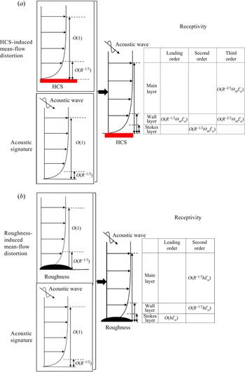
 $O(R^{-1/2}\varTheta _m {\mathcal {E}}_a)$, respectively (a detailed proof will be provided in § 3.5). Therefore, the leading-order receptivity is determined by the interaction in the wall layer, the second-order receptivity is determined by the Stokes-layer interaction, and the main-layer interaction appears only in the third-order receptivity. Note that it will be shown later that the higher-order wall-layer interaction also appears in the third-order receptivity, indicating that the third-order receptivity is determined by both the main-layer and wall-layer interactions. It also needs to be noted that even at third order, the non-parallelism of the Blasius solution is still negligible. A sketch of the interaction regime is provided in figure 2(a), and the detailed mathematics will be presented in § 3.5.
Sketch of the scaling estimate of the receptivity mechanism: (a) HCS–acoustic receptivity; (b) roughness–acoustic receptivity.

To this end, we are able to compare the present receptivity regime with that induced by the roughness–sound interaction (Dong et al. Reference Dong, Liu and Wu2020), whose scaling interaction is sketched in figure 2(b). In the latter regime, the three distinguished layers also appear, but the leading-order receptivity appears in the Stokes layer, which is  $O(h{\mathcal {E}}_a)$ and is attributed to the distortion of the acoustic signature by the curved wall, where
 $h\leq O(R^{-1/3})$ denotes the height of the roughness; the second-order receptivity appears in both the wall and main layers, which is
 $O(R^{-1/3}h{\mathcal {E}}_a)$ and is attributed to the nonlinear interaction between the mean-flow distortion and acoustic signature. Comparing the two regimes, we draw the following conclusions. (1) The leading-order contributors,
 $O(R^{-1/3}\varTheta _m{\mathcal {E}}_a)$ for the HCS cases, and
 $O(h{\mathcal {E}}_a)$ for the roughness cases, are essentially comparable, because for a nonlinear HCS and a nonlinear roughness element, we have assumed
 $\varTheta _m=O(1)$ and
 $h=O(R^{-1/3})$, respectively. (Note that the linear assumptions are made when
 $\varTheta _m\ll 1$ and
 $h\ll R^{-1/3}$.) (2) The leading-order contributors are driven by different mechanisms in different asymptotic layers. (3) The third-order contributor of the HCS cases is equivalent to the second-order contributor of the roughness cases, because they are both
 $O(R^{-1/3})$ smaller than the leading-order contributor and are driven by the same mechanism. (4) The second-order contributor of the HCS cases does not have a corresponding contributor in the roughness–acoustic receptivity.
3.2. HCS-induced mean-flow distortion
The streamwise length scale of the HCS is taken to be comparable with the local boundary-layer thickness. Actually, the asymptotic theory is valid for  $\varTheta _m\leq O(1)$, but numerical techniques are required to solve the nonlinear compressible boundary-layer equations when
 $\varTheta _m=O(1)$. For convenience of the asymptotic analysis, we assume the amplitude of the temperature of the HCS to be small, i.e.
 $\varTheta _m\ll 1$. The cases for
 $\varTheta _m=O(1)$ will be visited by employing the HLNS approach in § 5.5.
For demonstration, we assume the shape function of the temperature HCS to be
 \begin{equation}
f(x,z)=f_0(x)\cos(k_zz),\quad\text{with
}f_0(x)=\left\{\begin{array}{@{}ll} 1, & |x|\leq d/2, \\ 0, &
\text{otherwise}, \end{array} \right.
\end{equation}
where  $d=O(1)$ characterises the width of the HCS, and
 $k_z$ is the spanwise wavenumber of the HCS. The HCS is 2-D if
 $k_z=0$. Note that the choice of
 $f_0(x)$ here is only for demonstration, and in reality, the distribution at the two ends of the HCS,
 $x=\pm d/2$, should be rounded. Indeed, the amplitude of the excited instability mode relies on the Fourier transform of the distribution function only, and the choice of
 $f_0(x)$ does not affect the following analysis.
The mean flow distorted by the HCS exhibits a double-layered structure, as sketched in figure 2(a). For convenience, we introduce a small parameter
 \begin{equation} \epsilon=R^{{-}1/3}\ll 1. \end{equation}
3.2.1. Wall-layer solution
In the thin wall layer where  $y\sim \epsilon$, we introduce an
 $O(1)$ coordinate
 \begin{equation} Y=\epsilon^{{-}1}y. \end{equation}
Since  $\varTheta _m\ll 1$, the flow quantities can be expressed in terms of asymptotic series:
 $$\begin{gather} (\bar U,\bar
V,\bar W,\bar P,\bar T,\bar R)=\left(\epsilon\lambda
Y,0,0,\frac1{\gamma M^2},T_w(1+\epsilon
\lambda_TY),T_w^{{-}1}(1-\epsilon \lambda_T
Y)\right)\nonumber\\ {}+\frac{\varTheta_m}2(\epsilon
\bar U_0,\epsilon^2\bar V_0,\epsilon \bar W_0,\epsilon^2
T_w^{{-}1}\bar P_0,T_w(\bar T_0+\epsilon \bar
T_1),T_w^{{-}1}(\bar R_0+\epsilon\bar
R_1))\text{e}^{\text{i} k_zz}+\cdots+\text{c.c.},
\end{gather}$$
where  $\textrm {c.c.}$ denotes the complex conjugate,
 $\lambda \equiv U_{B,y}(0)$, and
 $\lambda _T\equiv T_{B,y}(0)/T_w$.
For  $\varTheta _m\ll 1$, the HCS-induced distortion
 $\bar \varPhi _0$ is to be solved in the spectrum space. We introduce the Fourier transform with respect to
 $x$:
 \begin{equation} \hat \varPhi^{\dagger}(k_x,y)={\mathcal{F}}[\bar \varPhi (x,y)]\equiv \frac{1}{\sqrt{2{\rm \pi}}}\int_{-\infty}^\infty \bar \varPhi(x,y)\,\text{e}^{-\text{i} k_x x}\,{\text{d}\kern0.06em x}. \end{equation}
Noticing that the mean-flow distortion is proportional to the spectrum of the shape function of the HCS,  $\hat f_0(k_x)={\mathcal {F}}[f_0(x)]$, we introduce
 \begin{equation} \hat \varPhi(k_x,y)=\hat \varPhi^{\dagger}(k_x,y)/\hat f_0(k_x). \end{equation}
For the shape function (3.2), we have
 \begin{equation} \hat f_0(k_x)=\frac{\text{i}}{\sqrt{2{\rm \pi}}k_x}(\text{e}^{-\text{i} k_xd/2}-\text{e}^{\text{i} k_x d/2}). \end{equation}
Substituting into the governing equations (2.3) and collecting the leading-order terms, we arrive at the linear system
 \begin{gather} \text{i} k_x(\hat U_{0}+\lambda Y\hat R_0)+\hat V'_0+\text{i} k_z\hat W_{0}=0, \end{gather}
 \begin{gather} \text{i} k_x\lambda Y\hat U_0+\lambda \hat V_0+\text{i} k_x\hat P_0=C_w(\hat U_{0}''+\lambda \mu_{T0}\hat T_0'), \end{gather}
 \begin{gather} \hat P_0'=0,\quad \text{i} k_x\lambda Y\hat W_0+\text{i} k_z\hat P_0=C_w\hat W_{0}'', \end{gather}
 \begin{gather} \text{i} k_x\lambda Y\hat T_0 =\frac{C_w}{Pr}\,\hat T_0'',\quad \hat T_0={-}\hat R_0, \end{gather}
 \begin{gather} \text{i} k_x\lambda Y\hat T_1-\frac{C_w}{Pr}\,\hat T_1''=\text{i} k_x{\lambda\lambda_T Y^2}\hat T_0+\frac{2\lambda_T C_w\mu_{T0}}{Pr}\,\hat T_0',\quad \hat T_1={-}\hat R_1, \end{gather}
where  $C_w=\mu _wT_w$, with
 $\mu _w=\mu (T_w)$. Throughout this paper, a prime denotes the derivative with respect to its argument, a hat represents the Fourier transformed quantity. Also,
 $k_x$ represents the streamwise wavenumber, and
 \begin{equation} \mu_{T0}=\left(\frac{\text{d}\mu}{\text{d}T}\right)_w\frac{T_w}{\mu_w} =\frac32-\frac{T_w}{T_w+\bar{\mathcal{C}}}. \end{equation}
This linear system is an extension of (5.3) in Dong et al. (Reference Dong, Liu and Wu2020) to the compressible-wall-layer configuration, and the boundary conditions remain the same. First, the no-slip, isothermal conditions are imposed at the wall. Second, for the cases with the HCS width comparable with boundary-layer thickness, the wall layer communicates with the main layer through an outflux velocity, and the displacement effect of the perturbation streamwise velocity as in the triple-deck theory becomes negligibly weak. The second boundary condition can also be found in Neiland et al. (Reference Neiland, Bogolepov, Dudin and Lipatov2008) for the roughness configuration, with its height and width being  $O(1)$ and
 $O(R^{-1/3})$, respectively. Therefore, the boundary conditions read
 \begin{gather} \hat U_0(0)=\hat V_0(0)=\hat W_0(0)=\hat T_1(0)=0,\quad \hat T_0(0)=1, \end{gather}
 \begin{gather} (\hat U_0,\hat W_0,\hat T_0,\hat T_1)\rightarrow 0\quad \text{as }Y\rightarrow \infty. \end{gather}
Solving (3.9e) with boundary conditions (3.11e,h), we obtain
 \begin{equation} \hat T_0(Y)=\mbox{Ai}(\bar\sigma Y)/\mbox{Ai}(0), \end{equation}
where Ai is the Airy function of the first kind, and  $\bar \sigma =({\textrm {i} k_x\lambda }\,Pr/{C_w})^{1/3}$. Differentiating (3.9d) with respect to
 $Y$, we arrive at an Airy equation of
 $\hat W_0'$, whose solution satisfying the boundary condition (3.11g) reads
 \begin{equation} \hat W_0(Y)={-}\frac{\text{i} k_z{\rm \pi}\hat P_0}{\sigma^2 C_w}\,\mbox{Gi}(\sigma Y)+C_0\,\mbox{Ai}(\sigma Y), \end{equation}
where  $\sigma =({\textrm {i} k_x\lambda }/{C_w})^{1/3}$,
 $\mbox {Gi}(\xi )={\rm \pi} ^{-1}\int _0^\infty \sin (t^2/3+\xi t)\,\textrm {d}t$, and
 $C_0$ is a constant. Applying the no-slip boundary condition (3.11c), we obtain
 \begin{equation} C_0=\frac{\text{i} k_z{\rm \pi}\hat P_0}{\sigma^2C_w}\,\frac{\mbox{Gi}(0)}{\mbox{Ai}(0)}\approx\frac{0.5774\,\text{i} k_z{\rm \pi}\hat P_0}{\sigma^2C_w}. \end{equation}
Differentiating (3.9b) with respect to  $Y$ and substituting (3.9a), we obtain
 \begin{align} \hat U_0'=\mbox{Ai}(\sigma
Y)\left(C_1\,{-}\,\frac{\rm \pi}{\sigma}\int_0^Y{\mbox{Bi}(\sigma
Y)\,g(Y)}\,\text{d}Y\right)\,{+}\,\mbox{Bi}(\sigma
Y)\left(C_2\,{+}\,\frac{\rm \pi}{\sigma}\int_0^Y{\mbox{Ai}(\sigma
Y)\,g(Y)}\,\text{d}Y\right)\!,
\end{align}
where Bi is the Airy function of the second kind,  $C_1$ and
 $C_2$ are two constants to be determined, and
 \begin{equation} g(Y)=\frac{ k_z^2\hat P_0\lambda{\rm \pi}}{\sigma^2 C_w^2}\left(0.5774\,\mbox{Ai}(\sigma Y)-\mbox{Gi}(\sigma Y)\right) +\frac{\lambda\sigma^3 (1-\mu_{T0}\,Pr)}{\mbox{Ai}(0)}\,Y\,\mbox{Ai}(\bar\sigma Y). \end{equation}
From the boundary condition (3.11f), we know that the exponentially growing part Bi $(\sigma Y)$ must be dropped in the limit of
 $Y\rightarrow \infty$, which leads to
 \begin{equation} C_2={-}\frac{\rm \pi}{\sigma}\int_0^\infty {\mbox{Ai}(\sigma Y)\,g(Y)}\,\text{d}Y\approx \frac{0.03563\, k_z^2\hat P_0\lambda{\rm \pi}^2}{\sigma^4 C_w^2} -\frac{0.2588\,{\rm \pi}\lambda (1-\mu_{T0}\,Pr)(1-Pr^{1/3})} {1-Pr}. \end{equation}
Applying (3.9b) at the wall, we obtain
 \begin{align} C_1=\frac{\text{i} k_x\hat P_0}{\sigma\,\mbox{Ai}'(0)\,C_w}-\frac{\mbox{Bi}'(0)\,C_2}{\mbox{Ai}'(0)}-\frac{\lambda\,Pr^{1/3}\,\mu_{T0} }{\mbox{Ai}(0)}\approx{-}\frac{\text{i} k_x\hat P_0}{0.2588\,\sigma C_w}+\sqrt{3}{C_2}-\frac{\lambda\, Pr^{1/3}\,\mu_{T0} }{0.3550}. \end{align}
Integrating (3.15) and applying the boundary condition (3.11f), we obtain
 $$\begin{gather} \frac{C_1}{\sigma}\int_0^\infty\mbox{Ai}(Y)\,\text{d}Y -\frac{\rm \pi}{\sigma}\int_0^\infty\mbox{Ai}(\sigma Y)\left(\int_0^Y{\mbox{Bi}(\sigma Y)\,g(Y)}\,\text{d}Y\right)\,\text{d}Y\nonumber\\ {}+\int_0^\infty\mbox{Bi}(\sigma Y)\left(C_2+\frac{\rm \pi}{\sigma}\int_0^Y{\mbox{Ai}(\sigma Y)\,g(Y)}\,\text{d}Y\right)\,\text{d}Y=0. \end{gather}$$
Solving numerically (3.17), (3.18) and (3.19), we can obtain  $C_1$,
 $C_2$ and
 $\hat P_0$.
Integrating the continuity equation (3.9a), we obtain the transverse velocity distortion
 \begin{equation} \hat V_0={-}\int_0^Y[\text{i} k_x(\hat U_0-\lambda Y\hat T_0)+\text{i} k_z \hat W_0]\,\text{d}Y. \end{equation}
In the limit of  $Y\rightarrow \infty$,
 \begin{equation} (\hat U_0,\hat
V_0,\hat W_0)\rightarrow (\hat C_u/Y,\hat C,\hat
C_w/Y)+\cdots,
\end{equation}
where
 \begin{equation} \hat C_u=\frac{ k_z^2 \hat P_0}{k_x^2\lambda},\quad\hat C_w={-}\frac{ k_z \hat P_0}{k_x\lambda},\quad \hat C={-}\frac{\text{i} k_x\hat P_0}{\lambda}\left(1+\frac{k_z^2}{k_x^2}\right). \end{equation}
Here,  $\hat C$ appears as the outflux from the wall layer to the main layer. It is seen that an HCS plays an equivalent role as a roughness element by inducing an outflux to the main layer. Especially for a 2-D HCS case (
 $k_z=0$), we find that both
 $\hat C_u$ and
 $\hat C_w$ are zero.
Additionally, the second-order temperature distortion reads
 \begin{align} \hat T_1=\mbox{Ai}(\bar\sigma Y)\left(\bar C_1-\int_0^Y\frac{{\rm \pi}\,\mbox{Bi}(\bar\sigma Y)\,\bar g(Y)}{\bar \sigma}\right)+\mbox{Bi}(\bar\sigma Y)\left(\bar C_2+\int_0^Y\frac{{\rm \pi}\,\mbox{Ai}(\bar\sigma Y)\,\bar g(Y)}{\bar \sigma}\,\text{d}Y\right), \end{align}
where  $\bar C_1$ and
 $\bar C_2$ are constants, and
 \begin{equation} \bar g(Y)={-}\frac{Pr}{\bar\sigma^2C_w}\left[\text{i} k_x{\lambda\lambda_T Y^2}\hat T_0+\frac{2\lambda_T C_w\mu_{T0}}{Pr}\,\hat T_0'\right]. \end{equation}
From the upper boundary condition, we obtain
 \begin{equation} \bar C_2={-}\frac{\rm \pi}{\bar \sigma}\int_0^\infty{\mbox{Ai}(\bar\sigma Y)\,\bar g(Y)}\,\text{d}Y, \end{equation}
whereas from the lower boundary condition, we obtain
 \begin{equation} \bar C_1={-}\bar C_2\,\mbox{Bi}(0)/\mbox{Ai}(0). \end{equation}
3.2.2. Main layer
The outflux  $\bar V=\epsilon ^2\varTheta _m\bar V_0$ from the wall layer is
 $O(\epsilon ^2\varTheta _m)$, which is actually the magnitude of the mean-flow distortion in the main layer. The analysis of the mean-flow distortion in the main layer is the same as in § 5.1.2 of Dong et al. (Reference Dong, Liu and Wu2020), and the asymptotic scalings can also be found in Neiland et al. (Reference Neiland, Bogolepov, Dudin and Lipatov2008). The velocity field, density, temperature and pressure of the mean flow in this layer are expressed as
 \begin{align} \bar\varphi=\left(U_B,0,0,\frac{1}{T_B},T_B,\frac{1}{\gamma M^2}\right)+\epsilon^2 \varTheta_m\hat C\left( U_{w1},V_{w1},W_{w1},R_{w1},T_{w1},P_{w1}\right)\frac{\text{e}^{\text{i} k_z z}}{2}+\cdots+\text{c.c.}, \end{align}
where  $\hat C=\hat C(k_x)$ has been defined in (3.21). Substituting into the NS equations (2.3) and retaining the
 $O(\epsilon ^2\varTheta _m)$ terms, we obtain governing equations for
 ${\boldsymbol {\varPhi }}_{w1}=( V_{w1}, P_{w1})$, which, under Fourier transform
 $\hat {\boldsymbol {\varPhi }}_{w1}(k_x,y)={\mathscr F}[{\boldsymbol {\varPhi }}_{w1}(x,y)]$, are expressed as
 \begin{equation} {\boldsymbol L}_R({\text{d}_y};\omega=0,k_x,k_z)\,\hat{\boldsymbol{\varPhi}}_{w1}=0, \end{equation}
where  ${\boldsymbol L}_R$ is the Rayleigh operator
 \begin{equation} \boldsymbol L_R(d_y;\omega,\alpha,\beta)=\boldsymbol I\,\frac{\text{d}}{\text{d} y}-\left(\begin{array}{@{}cc} {\text{i}\alpha U_B'}/{S_0} & [{-M^2S_0^2-T_B(\alpha^2+\beta^2)}]/{S_0} \\ -{S_0}/{T_B} & 0 \end{array}\right), \end{equation}
with  $S_0=\textrm {i}(\alpha U_B-\omega )$. The lower and upper boundary conditions read
 \begin{equation} \hat V_{w1}(0;k_x)=1,\quad k_y\hat P_{w1}+k_x\hat V_{w1}\rightarrow 0\ \text{as }y\rightarrow \infty, \end{equation}
where  $k_y=\pm [k_x^2(M^2-1)-k_z^2]^{1/2}$, with the negative and positive signs being selected for
 $k_x>0$ and
 $k_x<0$, respectively. The upper boundary condition represents a Mach wave radiating to the potential flow.
3.3. Acoustic signature
As sketched in figure 2, the boundary-layer response of freestream acoustic waves exhibits a double-layered structure: an inviscid main layer with  $y=O(1)$, and a viscous Stokes layer with
 $y=O(R^{-1/2})$. In the main layer, the perturbation is expressed as
 \begin{equation} \tilde{\boldsymbol\varphi}_{a}={\mathcal{E}}_a\,\hat{\boldsymbol\varphi}_{a0}(y)\,E_a\,\text{e}^{-\text{i}\omega t}+\cdots+\text{c.c.}, \end{equation}
where  ${\boldsymbol \varphi }=(v,p)^\textrm {T}$,
 ${\mathcal {E}}_a$ denotes its amplitude, and
 $E_a=\textrm {e}^{\textrm {i}(\alpha _ax+\beta _az)}$, with
 $\alpha _a$ and
 $\beta _a$ representing the streamwise and spanwise wavenumbers of the acoustic wave, respectively. The acoustic signature is governed by the unsteady Rayleigh equations
 ${\mathcal {L}}_R\hat {\boldsymbol \varphi }_{a0}=0$. The other quantities of the acoustic signature are expressed as
 \begin{equation} \left. \begin{aligned} & \hat u_{a0}=({-\text{i}\alpha_a T_B\hat p_{a0}-U_B'\hat v_{a0}})/{S_0}, \quad \hat w_{a0}={-\text{i}\beta_a T_B\hat p_{a0}}/{S_0},\\ & \hat \rho_{a0}={T_B'\hat v_{a0}}/({T_B^2S_0})+{M^2\hat p_{a0}}/{T_B},\quad \hat\theta_{a0}=(\gamma-1)M^2T_B\hat p_{a0}-{T_B'\hat v_{a0}}/{S_0}. \end{aligned} \right\} \end{equation}
The boundary condition at the wall is  $\hat v_{a0}(0)=0$, whereas in the freestream, the perturbation is a superposition of the incident and reflected acoustic waves,
 \begin{equation} \hat p_{a0}=\text{e}^{\text{i}\gamma_a y}+R_a\,\text{e}^{-\text{i}\gamma_a y}, \end{equation}
where  $\gamma _a$ denotes the wavenumber in the wall-normal direction, the amplitude of the incident component is set to be 1 for normalisation, and
 $R_a$ represents the amplitude of the reflected component. The dispersion relation of the acoustic wave reads
 \begin{equation} \omega=\left(1\pm\frac1{M\cos\theta}\right)\alpha_a, \end{equation}
where  $\theta$ represents its incident angle. The
 $\pm$ signs represent the fast and slow acoustic waves, respectively, because the phase speed
 $\omega /\alpha _a$ is faster and slower than the mainstream velocity, respectively. The incident wave must be propagating towards the wall, indicating a negative group velocity, i.e.
 $\textrm {d}\omega /\textrm {d}\gamma _a<0$. Therefore,
 $\gamma _a$ is positive for a slow acoustic wave and negative for a fast acoustic wave.
3.4. Mack instability
The double-deck structure for the acoustic signature is also valid for the Mack instability. In the main layer, the leading-order perturbation is governed by the Rayleigh equation
 \begin{equation} \boldsymbol L_R(d_y;\omega, k,\beta)(\hat v,\hat p)^\text{T}=0,\quad \hat p(\infty)\rightarrow 0. \end{equation}
In principle, the lower boundary condition should be the non-penetration condition to leading order,  $\hat v(0)=0$. However, as pointed out by Dong et al. (Reference Dong, Liu and Wu2020) and Dong & Zhao (Reference Dong and Zhao2021), the outflux of the underneath Stokes layer would induce an
 $O(R^{-1/2})$ correction. Although the magnitude of this correction is small, this term would include a factor
 $M^2$, which is quantitatively large for a hypersonic regime. Therefore, at a moderate Reynolds number, taking into account this correction would lead to a much more accurate prediction on the dispersion relation, as well as on the receptivity calculations. Therefore, we introduce a new parameter
 \begin{equation} \chi=R^{{-}1/2}M^2, \end{equation}
which could be  $O(1)$ at a moderate Reynolds number, but approaches zero as
 $R\to \infty$.
Taking into account the Stokes layer correction, we arrive at an improved boundary condition (Dong et al. Reference Dong, Liu and Wu2020),
 \begin{align} \hat v(0)&={-}\left(\frac{R}{C_w}\right)^{{-}1/2}\left[\frac{\text{i} (\gamma-1)\omega M^2}{(-\text{i}\omega\, Pr)^{1/2}}+\frac{(\alpha^2+\beta^2)T_w}{(-\text{i}\omega)^{3/2}}\right]\hat p(0)\nonumber\\ & ={-}\chi C_w^{1/2}\left[\frac{\text{i} (\gamma-1)\omega }{(-\text{i}\omega\, Pr)^{1/2}}+\frac{(\alpha^2+\beta^2)\bar T_w}{(-\text{i}\omega)^{3/2}}\right]\hat p(0), \end{align}
where  $\bar T_w=T_w/M^2$. For an adiabatic wall, the wall temperature
 $T_w$ is approximated by
 $T_{ad}=1+{Pr^{1/2}\,(\gamma -1)M^2}/{2}$, indicating that
 $\bar T_w$ can be assumed to be
 $O(1)$. For a cold (but not very cold) wall, such an approximation is also employed. Note that this improved boundary condition can also be applied to calculate the acoustic signature, but the improvement is rather limited because it is not an eigenvalue problem.
3.5. Excited perturbation
3.5.1. Main-layer solutions
In the receptivity process, the unsteady perturbation is a superposition of the acoustic signature and the excited perturbation induced by the HCS–acoustic interaction. In the main layer, they are expanded as
 \begin{align} \tilde{\boldsymbol\varphi}={\mathcal{E}}_a[\hat{\boldsymbol\varphi}_{a0}(y)\,E_a+\epsilon\varTheta_m\hat f_0(\tilde{\boldsymbol\varphi}_0+\epsilon^{1/2}\tilde{\boldsymbol\varphi}_1+\epsilon\tilde{\boldsymbol\varphi}_2+\cdots)\,\text{e}^{\text{i}\beta z}/2]\text{e}^{-\text{i}\omega t}+\cdots+\text{c.c.}, \end{align}
where  ${\boldsymbol \varphi }=(v,p)^\textrm {T}$, the subscript
 ${a0}$ denotes the acoustic signature, and the subscripts
 $0$, 1 and 2 represent the leading-, second- and third-order expansions of the excited perturbation. The magnitudes of the first three excited perturbations are estimated from the interactions between the acoustic signature and mean-flow distortion in the wall layer or in the Stokes layer, which will be demonstrated later. The excited perturbations under Fourier transform,
 $\hat { \boldsymbol \varphi }(y;k)={\mathcal {F}}[\tilde {\boldsymbol \varphi }(x,y)]$, satisfy
 \begin{gather} \boldsymbol L_R(d_y;\omega, k,\beta)\,\hat{\boldsymbol\varphi}_0=0; \end{gather}
 \begin{gather} \boldsymbol L_R(d_y;\omega, k,\beta)\,\hat{\boldsymbol\varphi}_1=0; \end{gather}
 \begin{gather} \boldsymbol L_R(d_y;\omega, k,\beta)\,\hat{\boldsymbol\varphi}_2=\hat C(k-\alpha_a)\,{\boldsymbol B}(\hat{\boldsymbol \varphi}_{a0},\hat{\boldsymbol{\varPhi}}_{w1}), \end{gather}
where the coefficient vector  ${\boldsymbol B}$ associated with the nonlinear interaction between the acoustic signature
 $\hat {\boldsymbol \varphi }_{a0}$ and the mean-flow distortion
 $\hat {\boldsymbol \varPhi }_{w1}$ is the same as that in Dong et al. (Reference Dong, Liu and Wu2020). As sketched in figure 2(a), the nonlinear interaction in the main layer is
 $O(\epsilon ^2 \varTheta _m {\mathcal {E}}_a)$, which appears only as a volumetric forcing in the third-order equation. Two types of the upper boundary conditions may be imposed. For a very-cold-wall configuration, the instability with a frequency close to the upper-branch neutral frequency would radiate acoustic wave to the far field, for which the perturbation fluctuates with a certain wall-normal wavenumber; see the boundary condition (36) of Zhao & Dong (Reference Zhao and Dong2022). For other cases, the perturbation attenuates in the far field, for which the boundary conditions to different orders read
 \begin{equation} (\hat p_0,\hat p_1,\hat p_2)\rightarrow 0\quad \text{as }y\rightarrow\infty. \end{equation}
In this paper, we do not take the wall temperature to be very low, and so the radiating mode is excluded in the following calculations. The wall boundary conditions read
 \begin{gather} \hat v_0(0)={\mathcal{G}}_0-(R/C_w)^{{-}1/2}\left[\frac{\text{i} (\gamma-1)\omega M^2}{(-\text{i}\omega\, Pr)^{1/2}}+\frac{(\alpha^2+\beta^2)T_w}{(-\text{i}\omega)^{3/2}}\right]\hat p_0(0), \end{gather}
 \begin{gather} \hat v_1(0)={\mathcal{G}}_1-(R/C_w)^{{-}1/2}\left[\frac{\text{i} (\gamma-1)\omega M^2}{(-\text{i}\omega\, Pr)^{1/2}}+\frac{(\alpha^2+\beta^2)T_w}{(-\text{i}\omega)^{3/2}}\right]\hat p_1(0), \end{gather}
 \begin{gather} \hat v_2(0)={\mathcal{G}}_2-(R/C_w)^{{-}1/2}\left[\frac{\text{i} (\gamma-1)\omega M^2}{(-\text{i}\omega\, Pr)^{1/2}}+\frac{(\alpha^2+\beta^2)T_w}{(-\text{i}\omega)^{3/2}}\right]\hat p_2(0), \end{gather}
where  ${\mathcal {G}}_{0}$,
 ${\mathcal {G}}_{1}$ and
 ${\mathcal {G}}_{2}$ denote the outflux obtained by analysing the underneath wall layer or Stokes layer, and the
 $O(R^{-1/2})$ terms are obtained by taking into account the viscous effect of the Stokes layer on the main layer (following (3.37)). Now our task is to solve for the outflux velocities
 ${\mathcal {G}}_{0}$,
 ${\mathcal {G}}_{1}$ and
 ${\mathcal {G}}_{2}$.
3.5.2. Wall-layer interaction
In the wall layer where  $y=O(\epsilon )$, the perturbation velocity field
 $(\tilde u_w,\tilde v_w,\tilde w_w)$, temperature
 $\tilde \theta _w$, density
 $\tilde \rho _w$ and pressure
 $\tilde p_w$ should match with the main-layer solutions asymptotically, which are expressed as
 \begin{align}
&{\mathcal{E}}_a\Bigg[(\hat u_{a00},\epsilon\hat
v'_{a00}Y,\hat w_{a00},\hat
\theta_{a00},\hat\rho_{a00},\hat p_{a00})E_a+\varTheta_m\hat f_0\sum_{k,\beta} (\hat
u_0+\epsilon^{1/2} \hat u_1+\epsilon \hat
u_2,\nonumber\\ &\quad \epsilon (\hat
v_0+\epsilon^{1/2} \hat v_1+\epsilon \hat v_2),\hat
w_0+\epsilon^{1/2}\hat w_1+\epsilon\hat w_1,\hat
\theta_0+\epsilon^{1/2}\hat \theta_1+\epsilon\hat
\theta_2,\nonumber\\ &\quad \quad
\hat\rho_0+\epsilon^{1/2}\hat \rho_1+\epsilon\hat
\rho_2,\epsilon(\hat p_0+\epsilon^{1/2}\hat
p_1+\epsilon\hat
p_2))\text{e}^{\text{i}(kx+\beta
z)}/2+\cdots\Bigg]\text{e}^{-\text{i}\omega
t}+\text{c.c.}, \end{align}
where  $\hat \varphi _{a00}=\hat \varphi _{a0}(0)$ and
 $\hat v_{a00}'=\textrm {d}\hat v_{a0}/{\textrm {d}y}|_{y=0}$. The three orders of
 $\hat v$ in the wall layer agree with the scaling estimate of the interaction regimes in figure 2. Note that the second-order inhomogeneous forcing,
 $O(\epsilon ^{3/2}\varTheta _m{\mathcal {E}}_a)$, should be from the thinner Stokes layer, and it will be shown that the wall layer acts as a ‘bridge’ to transmit the outflux from the Stokes layer to the main layer.
The leading-order excited perturbations are governed by
 \begin{gather} -\text{i} \omega T_w\hat\rho_0+\text{i} k\hat u_0+\hat v_0'+\text{i}\beta \hat w_0=\hat T_0(\text{i} k\hat u_{a00}+\hat v'_{a00}+\text{i}\beta\hat w_{a00})+\hat v_{a00}'Y\hat T_0', \end{gather}
 \begin{gather} -\text{i}\omega \hat u_0={-}\text{i}\omega\hat T_0\hat u_{a00},\quad\hat p_0'=0, \quad -\text{i}\omega\hat w_0={-}\text{i}\omega\hat T_0\hat w_{a00}, \end{gather}
 \begin{gather} -\text{i}\omega \hat\theta_0={-}\text{i}\omega \hat T_0\hat \theta_{a00}-\text{i} (k_x\hat u_{a00}+k_z\hat w_{a00})T_w\hat T_0-T_w\hat v_{a00}'Y\hat T_0', \end{gather}
 \begin{gather} T_w^2\hat \rho_0+\hat \theta_0={-}T_w^2\hat T_0\hat \rho_{a00}+\hat T_0\hat \theta_{a00}, \end{gather}
where  $\hat T_0=\hat T_0(y;k_x,k_z)=\hat T_0(y;k-\alpha _a,\beta -\beta _a)$. It is seen that this layer is inviscid. Noticing the relations of the acoustic signature (3.32), we obtain the solutions of (3.43):
 \begin{gather} \hat u_0=\frac{\alpha_a\hat T_0T_w\hat p_{a00}}{\omega},\quad\hat w_0=\frac{\beta_a\hat T_0T_w\hat p_{a00}}{\omega}, \end{gather}
 \begin{gather} \hat\theta_0=(\gamma-1)M^2T_w\hat T_0\hat p_{a00}+T_w\left(\frac{(k_x\alpha_a+k_z\beta_a)T_w\hat T_0\hat p_{a00}}{\omega^2}+\frac{Y\hat T_0'\hat v_{a00}'}{\text{i}\omega}\right), \end{gather}
 \begin{gather} \hat \rho_0={-}\frac{M^2\hat T_0\hat p_{a00}}{T_w}-\left(\frac{(k_x\alpha_a+k_z\beta_a)\hat T_0\hat p_{a00}}{\omega^2}+\frac{Y\hat T_0'\hat v_{a00}'}{\text{i}\omega T_w}\right){.} \end{gather}
Integrating (3.43a), and noticing that the transverse velocity in the underneath Stokes layer is at most  $O(\epsilon ^{3/2})$, which is negligible, we obtain
 \begin{equation} \hat v_0\rightarrow {\mathcal{G}}_0\quad\text{as }Y\rightarrow \infty, \end{equation}
where
 \begin{equation} {\mathcal{G}}_0={\mathcal{D}}_0\int_0^\infty\hat T_0\,\text{d}Y\,\hat p_{a00}\approx\frac{0.939\,{\mathcal{D}}_0(k_x)\,\hat p_{a00}}{(\text{i} \lambda k_x\,Pr/C_w)^{1/3}}, \end{equation}
with  ${\mathcal {D}}_0=-\textrm {i} (k\alpha _a+\beta \beta _a)T_w/\omega$. It determines the lower boundary condition of (3.39a).
The second-order perturbations in this layer are governed by the homogeneous linear system, which is the same as (3.43) but with the inhomogeneous terms on the right-hand side of each equation removed. However, there is an inhomogeneous forcing from the lower boundary, and so the transverse velocity is
 \begin{equation} {\mathcal{G}}_1=\hat v_1=\hat v_{10}, \end{equation}
where  $\hat v_{10}$ is the outflux from the underneath Stokes layer, to be obtained in the next subsection. Therefore, the wall layer only behaves as a bridge to transmit the outflux
 $\hat v_{10}$ to the lower boundary condition of the main-layer perturbations.
The third-order excited perturbations are governed by
 $$\begin{gather} -\text{i} \omega T_w\hat\rho_2+\text{i} k\hat u_2+\hat v_2'+\text{i}\beta \hat w_2=\hat T_1(\text{i} k\hat u_{a00}+\hat v'_{a00}+\text{i}\beta\hat w_{a00})+\hat v_{a00}'Y\hat T_1'\nonumber\\ {}-T_w\hat\rho_{a00}(\text{i} k \hat U_0+\hat V_0'+\text{i}\beta \hat W_0), \end{gather}$$
 $$\begin{gather}-\text{i}\omega \hat u_2+\text{i} kT_w\hat p_0={-}\text{i}\omega\hat T_1\hat u_{a00}-\text{i} k\hat U_0\hat u_{a00}-Y\hat v'_{a00}\hat U_0'-\text{i} \beta_a\hat W_0 \hat u_{a00}-\text{i} k_z \hat w_{a00}\hat U_0, \end{gather}$$
 $$\begin{gather}\hat p_2'=0, \end{gather}$$
 $$\begin{gather}-\text{i}\omega\hat
w_2+\text{i} \beta T_w\hat p_0={-}\text{i}\omega\hat
T_1\hat w_{a00}-\text{i} \alpha_a\hat U_0\hat
w_{a00}-\text{i} k_x\hat W_0\hat u_{a00}-Y\hat v_{a00}'\hat
W_0'-\text{i}\beta\hat W_0\hat
w_{a00},\nonumber\\ -\text{i}\omega
\hat\theta_2+\text{i}\omega(\gamma-1)M^2 T_w\hat
p_0={-}\text{i}\omega \hat T_1\hat \theta_{a00}-\text{i}
(k_x\hat u_{a00}+k_z\hat w_{a00})T_w\hat T_1\nonumber\\
{}-T_w\hat v_{a00}'Y\hat T_1'-\text{i}\alpha_a \hat U_0\hat
\theta_{a00}-\text{i} \beta_a\hat W_0\hat \theta_{a00}, \end{gather}$$
 $$\begin{gather}T_w^2\hat \rho_2+\hat \theta_2-\gamma M^2T_w\hat p_0={-}T_w^2\hat T_1\hat \rho_{a00}+\hat T_1\hat \theta_{a00}. \end{gather}$$
The solutions to these equations read
 \begin{equation} \left. \begin{aligned} \hat u_2 & =\frac{kT_w}{\omega}\,\hat p_0+\left[\frac{\alpha_a\hat T_1}{\omega}+ \frac{ k \alpha_a \hat U_0+\beta_a \alpha_a \hat W_0+ k_z\beta_a\hat U_0}{\omega^2}+ \left(\frac{M^{2}}{T_{w}}-\frac{\alpha_{a}^{2}+\beta_{a}^{2}}{\omega^{2}}\right) Y\hat{U}_0'\right]T_w\hat{p}_{a00},\\ \hat w_2 & =\frac{\beta T_w}{\omega}\,\hat p_0+\left[\frac{\beta_a\hat T_1}{\omega}+\frac{\beta_a\alpha_a\hat U_0+k_x\alpha_a\hat W_0+\beta\beta_a\hat W_0}{\omega^2}+\left(\frac{M^2}{T_w}-\frac{\alpha_a^2+\beta_a^2}{\omega^2}\right)Y\hat W_0'\right]T_w\hat p_{a00},\\ \hat \theta_2 & =(\gamma-1)M^2T_w\hat p_0+\left[\hat T_1+\frac{\alpha_a\hat U_0+\beta_a\hat W_0}{\omega}\right](\gamma-1)M^2T_w\hat p_{a00}\\ & \quad +\left({(k_x\alpha_a+k_z\beta_a)\hat T_1}+{\left[\frac{\omega^2M^2}{T_w}-(\alpha_a^2+\beta_a^2)\right]Y\hat T_1'}\right)\frac{T_w^2\hat p_{a00}}{\omega^2},\\ \hat \rho_2 & = \frac{M^2}{T_w}\,\hat p_0-\left[M^2\hat T_1+(\gamma-1)M^2\,\frac{\alpha_a\hat U_0+\beta_a\hat W_0}{\omega}\right]\frac{\hat p_{a00}}{T_w}\\ & \quad-\left({(k_x\alpha_a+k_z\beta_a)\hat T_1}+{\left[\frac{\omega^2M^2}{T_w}-(\alpha_a^2+\beta_a^2)\right]Y\hat T_1'}\right)\frac{\hat p_{a00}}{\omega^2}. \end{aligned} \right\} \end{equation}
Integrating (3.48a), we obtain
 \begin{equation} \hat v_2\rightarrow \left[\text{i}\omega M^2-\frac{\text{i}(k^2+\beta^2)T_w}{\omega}\right]\hat p_0Y+{\mathcal{G}}_2\quad\text{as }Y\rightarrow \infty, \end{equation}
where
 \begin{align} {\mathcal{G}}_2&= \left[{\mathcal{D}}_0\int_0^\infty\hat T_1\,\text{d}Y-\text{i}\left(\alpha_a(\gamma-1)M^2+\frac{T_w(k\alpha_a+\beta\beta_a)(k+\alpha_a) }{\omega^2}\right)\int_0^\infty\hat U_0 \,\text{d}Y\right.\nonumber\\ &\quad -\text{i}\left(\beta_a(\gamma-1)M^2+\frac{T_w (k\alpha_a+\beta\beta_a)(\beta+\beta_a) }{\omega^2}\right)\int_0^\infty\hat W_0 \,\text{d}Y-M^2\hat V_0\nonumber\\ &\left.\quad +\left(\frac{\alpha_a^2+\beta_a^2}{\omega^2}-\frac{M^2}{T_w}\right)\text{i} T_w( k\hat C_u+\beta \hat C_w)\vphantom{\int_0^\infty}\right]\hat p_{a00}. \end{align}
This leads to the wall boundary condition of (3.39c).
3.5.3. Stokes-layer interaction
Now we consider the Stokes layer where  $y=O(\epsilon ^{3/2})$. For convenience, we introduce a local coordinate
 \begin{equation} \bar Y=(R/C_w)^{1/2}y=O(1). \end{equation}
In this layer, the perturbation velocity field  $(\tilde u_S,\tilde v_S,\tilde w_S)$, temperature
 $\tilde \theta _S$, density
 $\tilde \rho _S$ and pressure
 $\tilde p_S$ are expressed as
 \begin{align}
&{\mathcal{E}}_a\,\text{e}^{-\text{i}\omega
t}\left[\vphantom{\sum_{k,\beta}}(\hat
u_{S},(R/C_w)^{{-}1/2}\hat v_S,\hat w_{S},\hat
\theta_{S},\hat\rho_{S},\hat p_{a00}
)E_a\right.\nonumber\\ &\quad
\left.{}+\varTheta_m\hat f_0\sum_{k,\beta} (\hat
U_S,(R/C_w)^{{-}1/2}\hat V_S,\hat W_S,\hat T_S,\hat
R_S,\epsilon\hat P_S)\text{e}^{\text{i}(kx+\beta
z)}/2\right]+\cdots+\text{c.c.},
\end{align}
where the acoustic-induced Stokes solutions read
 \begin{gather} (\hat u_S,\hat w_S)=(\alpha_a,\beta_a)\,\frac{T_w}{\omega}(1-\text{e}^{(-\text{i}\omega)^{1/2}\bar Y})\hat p_{a00}, \end{gather}
 \begin{gather} \hat \theta_S=M^2T_w(\gamma-1)(1-\text{e}^{(-\text{i}\omega\,Pr)^{1/2}\bar Y})\hat p_{a00}, \end{gather}
 \begin{gather} \hat\rho_S=\frac{M^2}{T_w}(1+(\gamma-1)\text{e}^{(-\text{i}\omega\,Pr)^{1/2}\bar Y})\hat p_{a00}, \end{gather}
with  $-\textrm {i}\equiv \textrm {e}^{3{\rm \pi} \textrm {i}/2}$. Here, we only probe the leading-order expansion, because the next-order excited perturbation of the transverse velocity should be
 $O(\epsilon ^{5/2}\varTheta _m{\mathcal {E}})$, producing only the fourth-order contribution to the receptivity efficiency.
Substituting (3.53) into the NS equations, we obtain, for each  $k\unicode{x2013} \beta$ spectrum, the linearised system
 \begin{gather} -\text{i} \omega T_w\hat R_S+\text{i} k\hat U_S+\hat V_S'+\text{i}\beta W_S=\text{i} k \hat u_S+\hat v_S'+\text{i}\beta\hat w_S, \end{gather}
 \begin{gather} -\text{i}\omega \hat U_S-\hat U_S''={-}\text{i}\omega \hat u_S+\mu_{T0}\hat u_S'',\quad\hat P_S'=0, \end{gather}
 \begin{gather} -\text{i}\omega \hat W_S-\hat W_S''={-}\text{i}\omega\hat w_S+\mu_{T0}\hat w_S'', \end{gather}
 \begin{gather} -\text{i}\omega \hat T_S-\frac{1}{Pr}\,\hat T_S''={-}\text{i}\omega \hat \theta_S-\text{i} T_w(k_x\hat u_S+k_z\hat w_S)+\frac{\mu_{T0}\theta_S''}{Pr}, \end{gather}
 \begin{gather} T_w^2\hat R_S+\hat T_S={-}T_w^2\hat \rho_S+\hat \theta_{S}, \end{gather}
where  $k_x=k-\alpha _a$, and
 $k_z=\beta -\beta _a$. The no-slip, non-penetration and isothermal conditions are imposed at the wall
 $\bar Y=0$. The solutions to (3.55) read
 $$\begin{gather} \hat U_S=\frac{T_w\alpha_a\hat p_{a00}}{\omega}\left[1-\text{e}^{(-\text{i}\omega)^{1/2}\bar Y}+\frac{(-\text{i}\omega)^{1/2}(\mu_{T0}+1)}{2}\,\bar Y\,\text{e}^{(-\text{i}\omega)^{1/2}\bar Y}\right], \end{gather}$$
 $$\begin{gather}\hat W_S=\frac{T_w\beta_a\hat p_{a00}}{\omega}\left[1-\text{e}^{(-\text{i}\omega)^{1/2}\bar Y}+\frac{(-\text{i}\omega)^{1/2}(\mu_{T0}+1)}{2}\,\bar Y\,\text{e}^{(-\text{i}\omega)^{1/2}\bar Y}\right],\end{gather}$$
 $$\begin{gather} \hat T_S=(\gamma-1)M^2T_w\hat p_{a00}\left[1-\text{e}^{(-\text{i}\omega\,Pr)^{1/2}\bar Y}+\frac{(-\text{i}\omega\, Pr)^{1/2}(\mu_{T0}+1)}{2}\,\bar Y\,\text{e}^{(-\text{i}\omega\,Pr)^{1/2}\bar Y} \right]\nonumber\\ +\frac{(k_x\alpha_a+k_z\beta_a)T_w^2\hat p_{a00}}{\omega^2}\left[1-\text{e}^{(-\text{i}\omega\,Pr)^{1/2}\bar Y}+\frac{Pr}{1-Pr}(\text{e}^{(-\text{i}\omega)^{1/2}\bar Y}-\text{e}^{(-\text{i}\omega\,Pr)^{1/2}\bar Y})\right]. \end{gather}$$
Integrating (3.55) from  $\bar Y=0$ to
 $\infty$, we obtain the outflux to the main layer
 \begin{equation} C_w^{1/2}\hat V_S\rightarrow O(\bar Y)+\hat v_{10}\quad \text{as }\bar Y\rightarrow \infty, \end{equation}
where
 \begin{align} \hat v_{10}&=\left[\frac{\text{i} (\alpha_a^2+\beta_a^2) (2-Pr) }{\omega(\sqrt{Pr}+1)}-\frac{\text{i}\omega M^2(\gamma-1)(1+\mu_{T0})}{2T_w}\right.\nonumber\\ &\left.\quad{}-\frac{\text{i} (k\alpha_a+\beta\beta_a) [4-2\,Pr+(\sqrt{Pr}+Pr)(\mu_{T0}+3)]}{2\omega(1+\sqrt{Pr})}\right]\frac{C_w^{1/2}T_w\hat p_{a00}}{(-\text{i}\omega\,Pr)^{1/2}}. \end{align}
This leads to the wall boundary condition of (3.47) and (3.39b).
3.6. Receptivity coefficients
The solutions for  $\hat {\boldsymbol \varphi }_0$,
 $\hat {\boldsymbol \varphi }_1$ and
 $\hat {\boldsymbol \varphi }_2$ in physical space are obtained by inverting the Fourier transform
 \begin{equation} \tilde{\boldsymbol\varphi}_l={\mathscr F}^{{-}1}[\hat{\boldsymbol\varphi}_l(k,y)]\equiv \frac1{\sqrt{2{\rm \pi}}}\int_{-\infty}^\infty \hat{\boldsymbol\varphi}_l(k,y)\,\text{e}^{\text{i} k x}\,\text{d}k,\quad l=0,1,2. \end{equation}
The integrand has a pole at  $k=\alpha$, where
 $\alpha$ is the wavenumber of a discrete mode. The integral in (3.59) may be evaluated by closing the integration contour in the upper half of the complex
 $k$-plane (Terent'ev Reference Terent'ev1981, Reference Terent'ev1984). The downstream perturbation is dominated by the contribution of the pole, and use of the residue theorem leads to
 \begin{equation} \tilde{\boldsymbol\varphi}_l\rightarrow\frac{\sqrt{2{\rm \pi}}\,\text{i}}{[\partial( \hat{\boldsymbol\varphi}_l)^{{-}1}/\partial k]_{k=\alpha}}\,\text{e}^{\text{i}\alpha x}\quad\text{as }x\rightarrow \infty. \end{equation}
Note that  $(\hat {\boldsymbol \varphi }_l)^{-1}$ for a vector
 $\hat {\boldsymbol \varphi }_l$ is a vector with each component being the reciprocal of the corresponding component in
 $\hat {\boldsymbol \varphi }_l$, which is evaluated by following the same approaches as in Dong et al. (Reference Dong, Liu and Wu2020). The exponential term on the right-hand side represents the growth of the excited eigenmode, and the prefactor is the equivalent amplitude at the centre of the HCS.
The receptivity can be quantified by an efficiency function
 \begin{equation} \varLambda_l=\lim_{x\rightarrow\infty}\tilde p_l(x,0)\,\text{e}^{-\text{i}\alpha x}=\frac{\sqrt{2{\rm \pi}}\,\text{i}}{[\partial \hat p_l^{{-}1}(k,0)/\partial k]_{k=\alpha}}, \end{equation}
which is independent of the distribution of the temperature at the HCS. The downstream perturbation pressure at the wall thus reads
 \begin{equation} \tilde{\boldsymbol p}\rightarrow {\mathcal{E}}_a\left[\hat{\boldsymbol p}_{a0}E_a+\frac{\epsilon \varTheta_m\hat f_0(\alpha-\alpha_a)}{2}\,(\varLambda_0+ \epsilon^{1/2}\varLambda_1+\epsilon\varLambda_2)\,\text{e}^{\text{i}(\alpha x+\beta z)}+\cdots\right]\text{e}^{-\text{i}\omega t}+\text{c.c.} \end{equation}
Combining the efficiency function at each order, we arrive at the receptivity coefficient
 \begin{equation} \varLambda=\varLambda_0+\epsilon^{1/2}\varLambda_1+\epsilon \varLambda_2+\cdots, \end{equation}
which is a quantity independent of the shape and intensity of the HCS.
4. Calculations at finite Reynolds numbers
In order to confirm the accuracy of the large- $R$ predictions, we carry out calculations at finite Reynolds numbers using two different approaches. The first is based on the compressible OS equations with inhomogeneous forcing considered, and is referred to as the extended OS (EOS) approach, which is valid only when
 $\varTheta _m\ll 1$. The second approach is the HLNS approach, which assumes only that the freestream acoustic waves and the excited Mack modes are infinitesimal and valid for any
 $\varTheta _m$.
4.1. EOS approach
This approach was first formulated by Zhigulev & Tumin (Reference Zhigulev and Tumin1987). For a linear HCS, the mean-flow distortion  $\bar { \boldsymbol {\varPhi }}$ in (3.1) depends linearly on
 $\varTheta _m$, which, in the spectrum space, is expressed as
 \begin{equation} \bar{\boldsymbol{\varPhi}}=T_w\varTheta_m\sum_{k_x}\hat f_0(k_x)\,\hat{ \boldsymbol{\varPhi}}_m\,\text{e}^{\text{i} (k_x x+k_z z)}+\text{c.c.} \end{equation}
Substituting (4.1) into the NS equations and neglecting the  $O(\varTheta _m^2)$ terms, we arrive at the steady OS equations
 \begin{equation} {\mathcal{L}}_{OS}({\text{d}_y};\omega=0,k_x,k_z,R)\,\hat{\boldsymbol\phi}_m=0, \end{equation}
where  ${\mathcal {L}}_{OS}$ denotes the compressible OS operator (Wu & Dong Reference Wu and Dong2016a), and
 $\hat {\boldsymbol \phi }=(\hat u,\hat u_{y},\hat v,\hat p,\hat \theta,\hat \theta _{y},\hat w,\hat w_{y})^\textrm {T}$. The wall boundary conditions read
 \begin{equation} \hat u_m(0)=\hat v_m(0)=\hat w_m(0)=0,\quad\hat \theta_m(0)=1. \end{equation}
The upper boundary condition, representing the radiated Mach waves, is the same as (3.8) of Dong et al. (Reference Dong, Liu and Wu2020).
The perturbation  $\tilde { \boldsymbol {\varPhi }}$ in (3.1) for an infinitesimal freestream acoustic wave (
 ${\mathcal {E}}_a\ll 1$) is expressed as
 \begin{equation} \tilde{ \boldsymbol{\varPhi}}={\mathcal{E}}_a(\hat{ \boldsymbol{\varPhi}}_a\,\text{e}^{\text{i}(\alpha_a x+\beta_a z)}+T_w\varTheta_m \hat{ \boldsymbol{\varPhi}}_e\,\text{e}^{\text{i}(k x+\beta z)})+\text{c.c.}, \end{equation}
where the subscripts  $a$ and
 $e$ represent the acoustic signature and excited perturbation, respectively. The acoustic signature also satisfies the compressible OS equations, which are subject to the boundary conditions
 \begin{equation} \hat u_a(0)=\hat v_a(0)=\hat w_a(0)=\hat \theta_a(0)=0, \end{equation}
and the same upper boundary conditions as (3.14) of Dong et al. (Reference Dong, Liu and Wu2020) (representing the incident and reflected acoustic waves).
The excited perturbation is governed by the inhomogeneous OS equations
 \begin{equation} {\mathcal{L}}_{OS}({\text{d}_y};\omega,k,\beta,R)\,\hat{\boldsymbol\phi}_{e}={\boldsymbol F}(\hat{\boldsymbol\phi}_a,\hat{\boldsymbol\phi}_m), \end{equation}
where the inhomogeneous forcing term  ${\boldsymbol F}$ is associated with the nonlinear interaction between the acoustic signature
 $\hat {\boldsymbol \phi }_a$ and the HCS-induced mean-flow distortion
 $\hat {\boldsymbol \phi }_m$; see Appendix A of Dong et al. (Reference Dong, Liu and Wu2020). The coupling conditions read
 $k_x\pm \alpha _a=k$ and
 $k_z\pm \beta _a=\beta$. Without loss of generality, we take the plus sign in the following.
Being the same as the asymptotic approach, the receptivity coefficient is given by
 \begin{equation} \varLambda_{EOS}=\frac{\sqrt{2{\rm \pi}}\,\text{i} T_w}{[\partial \hat p^{{-}1}_{e}(k,0)/\partial k]_{k=\alpha}}. \end{equation}
4.2. HLNS approach
The HLNS calculation includes two steps. First, we solve the full NS equations by an in-house code as in Zhao et al. (Reference Zhao, Dong and Yang2019), Zhao & Dong (Reference Zhao and Dong2020, Reference Zhao and Dong2022) and Dong & Zhao (Reference Dong and Zhao2021), to calculate the steady base flow. Second, we calculate the unsteady perturbation field  $\tilde \varphi$ by the HLNS approach (Zhao et al. Reference Zhao, Dong and Yang2019). This approach is applicable for both a weak (
 $\varTheta \ll 1$) and a strong (
 $\varTheta =O(1)$) HCS, in contrast to the EOS approach.
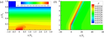
For a 2-D HCS, a rectangular computational domain  $[x_0,x_I]\times [0,y_J]$ is selected as shown in figure 3, and
 $(I+1)\times (J+1)$ grid points are employed. Here, we choose
 $(I,J)=(850,400)$, and a careful resolution study has been carried out. In the calculation of the mean flow for the first step, the convective and viscous terms of the NS equations are discretised by the fifth-order partial (using three upstream points and two downstream points) and fourth-order central finite difference schemes, respectively, whereas the third-order Runge–Kutta method is used for time advancing. In order to be comparable with the asymptotic predictions, the non-parallelism of the Blasius solution is neglected by introducing a body force as in Liu et al. (Reference Liu, Dong and Wu2020). The boundary conditions are set as follows. The compressible Blasius solution is set at the inlet of the computational domain
 $x_0$; the no-slip condition, non-penetration condition and isothermal condition (2.6) are imposed at the wall; a buffer region is introduced at the outlet
 $x_I$; the outflow condition is employed at the upper boundary
 $y_J$. The calculations continue until the solution converges to be time-independent, namely, the difference of the flow field between two neighbouring time steps is less than a certain threshold.
Sketch of the mesh system for the HLNS approach.

When the mean flow has been obtained by the first step, we can calculate the unsteady perturbation field  $\tilde \varphi$ (the second step) by solving the HLNS equation system. As illustrated in Zhao et al. (Reference Zhao, Dong and Yang2019), an infinitesimal perturbation with a given frequency
 $\omega$ can be expressed as
 \begin{equation} \tilde{\boldsymbol\varphi}={\mathcal{E}}_a\,\breve {\boldsymbol\varphi} (x,y)\,\text{e}^{\text{i} (\beta z-\omega t)}+\text{c.c.} \end{equation}
To ease the numerical process, we rearrange  $\breve {\boldsymbol \varphi }$ in terms of a Wentzel–Kramers–Brillouin form,
 $\breve {\boldsymbol \varphi }(x,y)=\textrm {e}^{\textrm {i}\alpha _0x}\,\breve {\boldsymbol \varphi }_0(x,y)$, where
 $\breve {\boldsymbol \varphi }_0$ varies slowly with
 $x$. Here,
 $\alpha _0$ is set to be the complex wavenumber obtained by the OS solution at
 $x=x_0$. Substituting (4.8) into the NS equation system and neglecting the
 $O({\mathcal {E}}_a^2)$ terms, we obtain a linear system
 \begin{equation} (\tilde{\boldsymbol{\mathsf{D}}}+\tilde{\boldsymbol{\mathsf{A}}}\partial_x+\tilde{\boldsymbol{\mathsf{B}}}\partial_y+\boldsymbol{\mathsf{V}}_{xx}\partial_{xx}+\boldsymbol{\mathsf{V}}_{yy}\partial_{yy}+\boldsymbol{\mathsf{V}}_{xy}\partial_{xy})\breve {\boldsymbol\varphi}_0(x,y)=0, \end{equation}
where the coefficient matrices  $\tilde {\boldsymbol{\mathsf{D}}}$,
 $\tilde {\boldsymbol{\mathsf{A}}}$,
 $\tilde {\boldsymbol{\mathsf{B}}}$,
 $\boldsymbol{\mathsf{V}}_{xx}$,
 $\boldsymbol{\mathsf{V}}_{yy}$ and
 $\boldsymbol{\mathsf{V}}_{xy}$ can be found in the Appendix of Zhao et al. (Reference Zhao, Dong and Yang2019). Under a proper discretisation, the system (4.9) is reduced to a system of linear algebraic equations.
At the inlet boundary, we introduce an acoustic-branch continuous mode of the OS equations,  $\hat { \boldsymbol {\varPhi }}_a$ (defined in (4.4)), representing the boundary-layer response to the acoustic forcing. For normalisation, we set the pressure amplitude of the incident acoustic mode to be unity. The wall and upper boundary conditions are the same as for the EOS approach, and the outflow condition is set at the outlet boundary.
Solving the linear system (4.9) with the aforementioned boundary conditions, we obtain the perturbation field  $\breve {\boldsymbol \varphi }$, which includes both the acoustic signature
 $\breve {\boldsymbol \varphi }_a$ and the excited perturbations
 $\breve {\boldsymbol \varphi }_e$. The latter eventually evolves into the Mack mode in the downstream limit. Therefore, the receptivity coefficient
 $\varLambda$ is calculated by the amplitude of the excited Mack-mode pressure at the HCS normalised by
 $\varTheta _m\hat f_0(\alpha -\alpha _a)$, since the amplitude of the oncoming perturbation is set to be unity.
5. Numerical results
5.1. Base flow and its linear instability
In this paper, the receptivity calculations are performed for four cases with different  $M$ and
 $T_w$, as listed in table 1. In the table, the detailed parameters are given, including the ratio of the wall temperature
 $T_w$ to the adiabatic wall temperature
 $T_{ad}$, the displacement and nominal boundary-layer thicknesses (
 $\delta _1$,
 $\delta _{99}$), the location of the generalised inflectional point (GIP)
 $y_c$, and the velocity
 $U_c$ at the GIP. All these cases were also studied in Zhao & Dong (Reference Zhao and Dong2022), although in that paper the reference length was chosen to be
 $\delta _1$.
Parameters for case studies.

The  $U_B$ and
 $T_B$ profiles of the base flow are shown in figure 4. For the same
 $M$, the boundary-layer thickness
 $\delta _{99}$ decreases with decrease of
 $T_w$, whereas for adiabatic walls,
 $\delta _{99}$ increases with
 $M$. It is seen clearly that in the near-wall region,
 $U_B$ for each case shows a linear dependence of
 $y$ in a rather wide transverse region, confirming the approximation of
 $\bar U$ in (3.5). However, the approximation of
 $\bar T$ in (3.5),
 $T_w(1+\epsilon \lambda _T Y)$, is valid in a much thinner region adjacent to the wall, and the lower
 $T_w$, the greater the error of the approximation at a certain transverse location. This may lead to a greater error for the calculations of the mean-flow distortion for a lower
 $T_w$. Note that if
 $T_w$ is taken to be much smaller than unity, then the main deck splits into two distinguished layers, as shown in Cassel, Ruban & Walker (Reference Cassel, Ruban and Walker1996). However, such a cold-wall effect does not appear in our study because we focus only on
 $T_w>1$; see table 1.
Profiles of (a)  $U_B$ and (b)
 $T_B$ of the compressible Blasius solution for the four cases.

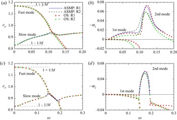
The symbols in figure 5(a) show the OS solutions of the phase speed of the fast and slow modes for case 1. They originate from the phase speeds of the fast and slow acoustic waves with zero incident angle,  $1+1/M$ and
 $1-1/M$, respectively, and intersect at
 $\omega \approx 0.11$ for both
 $R=7800$ and 1560, which is referred to as the synchronisation frequency. The curves show the phase speeds of the slow mode obtained by the asymptotic prediction (3.35) with (3.37), which agree well with the OS calculations. The growth rate of the slow mode, plotted in figure 5(b), shows overall two peaks, the frequencies of which correspond to the most unstable state of the first and second modes, respectively. For this case, the two unstable zones intersect at around
 $\omega =0.1$, for which the growth rate
 $-\alpha _i$ is positive. Increase of
 $R$ leads to a destabilising effect. The asymptotic predictions of the growth rate are close to the OS calculations, and the agreement is better for a higher
 $R$. Figures 5(c,d) show the results for case 3. Only the second mode for the Reynolds numbers considered is unstable, and the agreement between the asymptotic predictions and OS calculations is quite satisfactory. These plots can also be found in Zhao & Dong (Reference Zhao and Dong2022), but the reference lengths of the two papers are different.
Dependence on  $\omega$ of (a,c)
 $c_r$ and (b,d)
 $-\alpha _i$ of the 2-D Mack modes, where the velocities of the fast and slow acoustic waves,
 $1\pm 1/M$, are marked in (a,c). Plots for (a,b) case 1, and (c,d) case 3. R1 and R2 are for
 $R=7800$ and 1560, respectively. The abbreviations ASMP and OS denote the asymptotic predictions and the OS solutions, respectively.

5.2. Mean-flow distortion induced by the HCS
Solving numerically (3.12), (3.13), (3.15) and (3.20), we obtain the mean-flow distortion in the wall layer, and figure 6 displays the profiles for a representative configuration. The inhomogeneous forcing induces a temperature distortion from the wall, which damps exponentially as  $Y$ becomes large, agreeing with the distribution of the Airy function. The distortion of the transverse velocity
 $\hat V_0$ tends to a constant
 $\hat C$ (shown by the green dashed lines in figure 6a) in the limit of
 $Y\rightarrow \infty$, which agrees with the analytical prediction (3.21b). The large-
 $Y$ behaviours of
 $\hat U_0$ and
 $\hat W_0$ can be predicted by (3.21a) and (3.21c), both of which decay algebraically like
 $1/Y$. It is also predicted that for
 $k_x=k_z$, the prefactors are
 $\hat C_u=-\hat C_w$, which are clearly confirmed by figure 6(b). If
 $k_z$ is set to be zero, then the profiles of
 $\hat V_0$ and
 $\hat T_0$ do not change, but
 $\hat W_0$ becomes zero, and
 $\hat U_0$ changes its large-
 $Y$ asymptotic behaviour because
 $\hat C_u=\hat C_w=0$ (which are not shown here for brevity). Remarkably, only the constant
 $\hat C=\hat V_0(\infty )$ is able to communicate with the main layer, which generates an outflux with an order of magnitude
 $O(R^{-2/3}\varTheta )$, as indicated in (3.30a).
Profiles of the mean-flow distortion in the wall layer for case 1 with  $k_x=k_z=0.028$: (a)
 $\hat V_0$ and
 $\hat T_0$ profiles; (b)
 $\hat U_0$ and
 $\hat W_0$ profiles. The dashed lines denote the asymptotic estimations.

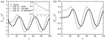
The mean-flow distortion in the main layer is obtained by solving numerically (3.28) with (3.30). In figure 7, we show the normalised profiles of  $\hat V_{w1,r}$ and
 $\hat P_{w1,r}$ for a representative configuration by the circles. In the freestream, the profiles oscillate with wavelength approximately 40, indicating a Mach wave radiating to the far field. Solving the OS equation (4.2) with (4.3) and the upper-boundary radiation boundary condition, we are able to predict the same profiles at finite Reynolds numbers. The relation between the two solutions is
 $(\hat V_{w1},\hat P_{w1})=T_wR^{-2/3}(\hat v_m,\hat p_m)$. The OS solutions for three
 $R$ values are also plotted in figure 7. It is seen clearly that the OS solutions approach the asymptotic predictions as
 $R$ increases. Even for the highest-
 $R$ case, we can still see a discrepancy of
 $\hat V_{w1}$ in the near-wall region, because the main-layer asymptotic theory ceases to be valid there. Note that in this region, the agreement of the pressure distortion is still good, which is because
 $\hat P_{w1}$ stays constant to leading order in the thin wall layer. A better comparison can be made by constructing a composite solution from the asymptotic theory,
 \begin{equation} \hat V_{com}(y)=\hat V_{w1}(y)+\hat V_0(\epsilon^{{-}1}y)-\hat C. \end{equation}
Normalised profiles of the real parts of (a)  $\hat V_{w1}$ and (b)
 $\hat P_{w1}$ in the main layer for case 1 with
 $k_x=0.028$ and
 $k_z=0$. The inset in (a) shows a zoom-in plot in the near-wall region.

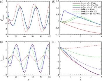
Figure 8(a) compares  $\hat V_{com}$ with the OS solutions
 $T_w R^{-2/3}\hat v_m$ for the three
 $R$ values, and figure 8(b) shows its zoom-in plot in the near-wall region. As
 $R$ increases, the wall layer becomes thinner with scale
 $\epsilon y$, and the agreement between the asymptotic predictions and OS solutions becomes better in both the main and wall layers. Figures 8(c,d) show the comparison for case 3, an extremely cold wall case. Again, the agreement between the two families of curves becomes better as
 $R$ increases. However, at a moderate
 $R$, i.e.
 $R=156\,000$, the agreement is much worse than that for case 1, especially in the near-wall region. The implication is that for the same Reynolds number, the asymptotic prediction at a cold-wall configuration is less accurate, probably due to the less accurate assumption of the base-flow temperature profile in the wall layer at a finite
 $R$, as indicated in figure 4. Such an error may be directed to the receptivity calculations.
Comparison of the distortion of the transverse velocity between the asymptotic composite solution (solid lines) and the EOS solutions (dot-dashed lines) for  $k_x=0.028$ and
 $k_z=0$: (a,b) case 1, and (c,d) case 3. Panels (b,d) show zoom-in plots of (a,c) in the near-wall region, respectively.

5.3. Receptivity
The boundary-layer response to the freestream sound waves, including the fast and slow acoustic modes, is the same as that in Dong et al. (Reference Dong, Liu and Wu2020), and so is not repeated in this paper. In the following, we will present the numerical predictions of the receptivity efficiency and confirm their accuracy by finite- $R$ calculations.
5.3.1. Asymptotic predictions of the receptivity efficiency
According to the asymptotic theory presented in § 3, the effects of the HCS distribution and instability property on the receptivity are readily separated, namely, the excited perturbation depends on the product of the Fourier transform of the HCS distribution  $\hat f_0(\alpha -\alpha _a)$ and the receptivity coefficient
 $\varLambda$. For a locally uniform HCS, the former is given by (3.8), so in this subsubsection, we focus only on the latter.
In figure 9(a), we show the dependence on  $\omega$ of the efficiency functions to freestream fast acoustic waves with incident angle
 $\theta =45^\circ$ and
 $\beta _a=0$ for case 1, where two representative Reynolds numbers are considered. Because, for these configurations, the first-mode and second-mode unstable regions connect to each other, the plot includes both frequency bands. Overall, we can see a peak for each order of
 $\varLambda$ at
 $\omega \approx 0.105$, close to the intersection frequency of the first and second modes. For lower frequencies,
 $\varLambda$ to each order damps rapidly with decrease of
 $\omega$, indicating a rather weak receptivity efficiency of the first mode; for higher frequencies, the damping rate with increase of
 $\omega$ is much slower, showing a broad frequency band for significant receptivity. The implication is that the receptivity to this fast acoustic forcing of the second mode is more important than that of the first mode. Because
 $\varLambda _2$ is one order of magnitude greater than
 $\varLambda _0$ and
 $\varLambda _1$, the blue
 $\varLambda _2$ curves are multiplied by a factor 0.1 for plotting convenience. The large-
 $\varLambda _2$ feature determines that at a rather moderate Reynolds number, the leading-order asymptotic prediction may yield an appreciable error in comparison with the finite-
 $R$ and direct numerical simulation calculations, therefore a reasonable prediction should include the efficiency function of the first three orders. It needs to be noted that although
 $\epsilon \varLambda _2$ may be quantitatively greater than
 $\epsilon ^{1/2}\varLambda _1$ at a moderate Reynolds number, the asymptotic expansion is still valid because
 $\varLambda$ to each order is independent of
 $\epsilon$. In the second-mode frequency band, increase of
 $R$ leads to a stronger receptivity at each order. Figure 9(b) shows the receptivity to freestream slow acoustic waves with the same configurations. Overall, the curves show a similar trend as those in figure 9(a), except for the following three points: first, the
 $\varLambda$ value to each order is smaller; second, in the second-mode frequency band,
 $\varLambda _1$ and
 $\varLambda _2$ vary more gently; third,
 $\varLambda _2$ in the low-frequency limit shows a trend of blow-up. These features agree with those for the roughness–acoustic receptivity as in Dong et al. (Reference Dong, Liu and Wu2020).
Asymptotic predictions of the efficiency function at each order at different frequencies for the receptivity to a 2-D freestream acoustic wave with incident angle  $\theta =45^\circ$: (a,c,e,g) fast acoustic forcing; (b,d, f,h) slow acoustic forcing. Plots for (a,b) case 1, (c,d) case 2, (e, f) case 3, and (g,h) case 4. For plotting convenience, the blue curves for
 $|\varLambda _2|$ are multiplied by 0.1.

In figures 9(c,d), we plot the  $\varLambda$ curves for case 2. Because the first-mode and second-mode frequency bands do not join together for this case, and the receptivity of the second mode is stronger, the plot includes only the second-mode frequency band. The receptivity to the fast acoustic forcing peaks around the lower-branch neutral frequency. However, for the receptivity to the slow acoustic forcing, another peak in the upper-branch frequency band appears, which is even stronger than the lower-branch peak for
 $\varLambda _2$. From the physical point of view, the receptivity near the lower-branch neutral point is more interesting due to its successive amplification in a broad downstream region. For an even lower wall temperature, as shown in figures 9(e, f) for case 3, the two peaks around the lower- and upper-branch neutral frequencies are seen clearly. Comparing cases 1, 2 and 3, which are with the same
 $M$, we find that as
 $T_w$ decreases, the values of
 $\varLambda$ to each order increases, especially
 $\varLambda _2$, indicating a stronger receptivity efficiency. Additionally, the lower the wall temperature
 $T_w$, the greater
 $|\varLambda _2|/|\varLambda _0|$, indicating an increasingly important role of the third-order receptivity as
 $T_w$ decreases.
In figures 9(g,h), we show the  $\varLambda$ curves for case 4,
 $M=4.5$ with an adiabatic wall. Again, for both the fast and slow acoustic forcing, the strongest receptivity efficiency at each order appears near the lower-branch neutral frequency. Compared with case 1, it is found that in the second-mode frequency band, the receptivity to the fast acoustic wave is stronger for a lower Mach number, while the magnitude of the receptivity efficiency to the slow acoustic wave does not evidently change with the Mach number. Since the receptivity to fast acoustic waves is stronger, we show the dependence of the efficiency function on the incident angle of 2-D fast acoustic waves for the four cases in figure 10, where the frequencies are chosen to be around the lower-branch neutral frequencies. For each order,
 $\varLambda$ shows a peak at a certain
 $\theta$, and decays drastically as
 $\theta$ approaches 0 or
 $90^\circ$. The most efficient angle is within
 $30<\theta <60$, and increase of
 $R$ does not affect this efficient angle. Setting the freestream fast acoustic wave to be three-dimensional, and with fixed incident angle
 $45^\circ$, we show the receptivity efficiency for a 2-D HCS for the four cases in figure 11. The frequency of the incident acoustic wave for each case is around the lower-branch neutral frequency, and only the unstable spanwise wavenumber band (
 $\beta =\beta _a$) is shown. For case 1, shown in figure 11(a),
 $\varLambda$ increases with
 $\beta _a$ rather mildly, except for
 $\varLambda _2$ with
 $R=1560$. After peaking at a certain
 $\beta _a$,
 $\varLambda$ decays drastically with
 $\beta _a$. As the wall temperature decreases, shown in figures 11(b,c), the peaking
 $\beta _a$ becomes greater, which even disappears in the unstable wavenumber band for case 3 (the extremely cold wall). Comparing figures 11(a,d), we find that as
 $M$ decreases, the unstable
 $\beta _a$ band shrinks, and the drastic decay of
 $\varLambda$ on
 $\beta _a$ in the high-
 $\beta _a$ band disappears. Again, we can see a stronger receptivity efficiency for a lower Mach number.
Dependence of the efficiency function on the incident angle of the 2-D freestream fast acoustic wave. The line types are the same as in figure 9, and the blue curves for  $\varLambda _2$ are multiplied by 0.1. Plots for (a) case 1 with
 $\omega =0.108$; (b) case 2 with
 $\omega =0.126$; (c) case 3 with
 $\omega =0.153$; (d) case 4 with
 $\omega =0.185$.

Dependence of the efficiency function on the spanwise wavenumber of the freestream fast acoustic wave  $\beta _a$, where
 $k_z=0$ and
 $\theta =45^\circ$. The line types are the same as in figure 9, and the blue curves for
 $\varLambda _2$ are multiplied by 0.1. Plots for (a) case 1 with
 $\omega =0.108$; (b) case 2 with
 $\omega =0.126$; (c) case 3 with
 $\omega =0.153$; and (d) case 4 with
 $\omega =0.185$.

5.4. Comparison of the receptivity efficiency between the asymptotic predictions and the EOS solutions
To confirm the accuracy of our asymptotic predictions, we compare them with the EOS solutions  $\varLambda _{EOS}$ for representative configurations in figure 12. All the plots indicate the same feature, namely, the leading- and second-order asymptotic predictions are not sufficient, and the predictions made by the first three orders of
 $\varLambda$ show rather better agreement with the EOS solutions. For adiabatic walls (cases 1 and 4), the asymptotic predictions are rather accurate even when
 $R=O(1000)$, while the prediction at a finite
 $R$ becomes poorer as
 $T_w$ decreases. This is due to the less accurate prediction of the mean-flow distortion as illustrated in figure 8. The solid lines and circles in figure 13 compare the receptivity coefficient
 $\varLambda$ obtained by the EOS solutions and the asymptotic predictions for different
 $\omega$. When the unstable regions of the first and second modes merge, i.e. case 1, the receptivity coefficient peaks at the synchronisation frequency; when the two unstable regions separate, i.e. case 4, the receptivity coefficient peaks near the the lower-branch neutral frequency of the second mode. In the asymptotic predictions, the first three orders of the efficiency functions are taken into account, i.e.
 $\varLambda =\epsilon (\varLambda _0+\epsilon ^{1/2}\varLambda _1+\epsilon \varLambda _2)$. The two families of curves agree with each other overall, and the agreement is better for a greater Reynolds number.
Comparison of the receptivity coefficient  $\varLambda$ between the EOS solutions and the asymptotic predictions for different
 $R$. The freestream perturbation is the fast acoustic wave with
 $\theta =45^\circ$. Leading order is
 $\epsilon \varLambda _0$; two orders is
 $\epsilon (\varLambda _0+\epsilon ^{1/2}\varLambda _1)$; three orders is
 $\epsilon (\varLambda _0+\epsilon ^{1/2}\varLambda _1+\epsilon \varLambda _2)$. Plots for (a) case 1, (b) case 2, (c) case 3, and (d) case 4. For plotting convenience, the curves for
 $\omega =0.145$ and 0.160 in (b) are multiplied by 0.1 and 0.01, respectively; those for
 $\omega =0.175$ and 0.190 in (c) are multiplied by 0.1 and 0.01, respectively; those for
 $\omega =0.224$ in (d) are multiplied by 0.1.

Comparison of the receptivity coefficient  $\varLambda$ between the EOS solutions and the asymptotic predictions for different
 $\omega$: (a) case 1, (b) case 4.

5.5. Validation of the asymptotic predictions by the HLNS calculations
We further compare the asymptotic predictions with the HLNS calculations in this subsection. The oncoming conditions are selected from case 4 in table 1 and  $R=1560$; the freestream forcing is the fast acoustic waves with the same incident angle,
 $\theta =45^\circ$, but different frequencies. The HCS has the same width and intensity, namely,
 $d=0.5\delta _{99}=6.76$ and
 $\varTheta _m=0.1$.
Figures 14(a,b) show the temperature and pressure contours of the mean flow distorted by a heating source with  $(\varTheta _m,d)=(0.1,6.76)$, respectively. Due to the localised surface heating, a high-temperature region appears in the region
 $x/\delta _1\in (-0.5,0.5)$ and
 $y/\delta _1\in [0,0.2)$, and a Mach wave, showing a peak of the pressure distortion, is radiated to the far field. These observations agree with the asymptotic solutions in figures 6 and 7.
Contours of the mean (a) temperature and (b) pressure distorted by a heating source with  $d/\delta _1=0.65$ and
 $\varTheta _m=0.1$.

We introduce an acoustic wave with  $\theta =45^\circ$ and
 $\omega =0.178$ to the mean flow shown in figure 14, then we calculate the perturbation field using the HLNS approach. The obtained pressure contours are shown in figure 15(a i). The introduced acoustic frequency corresponds to the lower-branch neutral frequency of the Mack second mode. From this plot, we can see only the propagation of the acoustic signature, which is oscillatory in the external stream and shows a peak in the near-wall Stokes layer. In figure 15(a ii), we subtract out the oncoming acoustic signature
 $\breve p_a$, obtained by calculating the acoustic field without an HCS, and plot the contours only for the excited perturbation pressure defined by
 $\breve p_e=\breve p-\breve p_a$. Because the excited Mack second mode is almost neutral, the downstream perturbation shows a neutrally oscillatory feature. Additionally, the HCS induces a Mach wave radiating to the far field (see figure 14b), which leads to a weak distortion of the acoustic wave in the downstream region. Such a phenomenon can also be interpreted as a weak scattering effect on the freestream acoustic wave, so in the potential region downstream of the Mach wave, the acoustic field includes both the oncoming acoustic field
 $\breve p_a$ and the weak scattering field. The latter is referred to as the residual acoustic perturbation, which is retained in
 $\breve p_e$. Therefore, we can see the weak modulation of the second mode by the residual acoustic perturbation in the downstream boundary-layer region (see also figure 16(a) for
 $\breve p_e(x,0)$). This phenomenon can also be seen in the simulations of Dong & Li (Reference Dong and Li2021).
Contours of (a i,b i) the perturbation pressure  $\breve p$, and (a ii,b ii) the excited perturbation pressure
 $\breve p_e=\breve p-\breve p_a$, for (a)
 $\omega =0.178$, and (b)
 $\omega =0.202$.

Streamwise evolution of the excited pressure perturbation at the wall  $\breve p_e(x,0)$, for (a)
 $\omega =0.178$, and (b)
 $\omega =0.202$.

In figures 15(b i,b ii), we show the same plots for  $\omega =0.202$, corresponding to the most unstable frequency of the second mode. The evolution of the whole perturbation pressure
 $\breve p$ remains similar to that in figure 15(a i), but as shown in figure 15(b ii), the excited perturbation shows an exponential growth in the downstream limit. Because the ‘residual’ acoustic perturbation is almost neutral, much weaker than the exponential growing Mack mode, the modulation induced by the acoustic wave (as shown by the streamwise evolution of
 $\breve p_e(x,0)$ in figure 16b) is not as strong as that for the neutral case.
In order to obtain the receptivity coefficient, we need to measure the initial amplitude of the excited Mack-mode pressure, which is difficult due to the contamination of the acoustic modulation. In order to exclude this effect, we employ the mode decomposition technique as in Tumin (Reference Tumin2003) and Gao & Luo (Reference Gao and Luo2014). Using the adjoint vector of the OS system, we are able to obtain the ‘Mack-mode part’ of the downstream perturbation  $\breve p_M$, as shown in figure 17(a). In the downstream limit, the unstable Mack modes with frequencies 0.182 and 0.202 grow exponentially, while the neutral Mack mode with
 $\omega =0.178$ stays almost constant. If each curve is normalised by the linear evolution of the Mack instability with the same frequency, then the downstream amplitudes are all constant, as shown in figure 17(b). These downstream constants represent the equivalent initial amplitudes of the excited Mack modes, also referred to as the receptivity coefficients. The comparison of
 $\varLambda$ between the asymptotic predictions and the HLNS calculations is shown in figure 18, where different HCS intensities are included. For both the heating and cooling sources, the overall trend of the dependence of
 $\varLambda$ on
 $\omega$ is the same for the two families of curves, confirming the accuracy of the asymptotic predictions.
Streamwise evolution of (a) the mode-decomposition amplitude  $|\breve p_M(x,0)|$, and (b) its normalisation by its linear evolution
 $|\breve p_M(x,0)/\exp (\textrm {i}\alpha x)|$.

Comparison of the receptivity coefficient  $\varLambda$ between the asymptotic predictions and the HLNS calculations: (a) heating source with
 $\varTheta _m>0$; (b) cooling source with
 $\varTheta _m<0$.

An interesting observation from figure 18 is that even when the HCS intensity reaches  $|\varTheta |=0.8$, i.e. the relative temperature deviation at the HCS reaches
 $80\,\%$, the nonlinear effect is still not strong enough to induce an apparent change of the normalised receptivity coefficient. A further plot for the dependence of the excited perturbation amplitude by unity acoustic forcing,
 $K=\varLambda \varTheta _m\hat f_0(\alpha -\alpha _a)$, on the HCS intensity is shown in figure 19, in which the linear predictions, obtained by extending directly the results for
 $\varTheta _m=0.1$, are plotted by the dashed lines. For each frequency, as
 $|\varTheta _m|$ increases, the receptivity coefficient agrees overall with the linear prediction, and the nonlinearity slightly weakens the receptivity in comparison with the linear predictions for both the heating and cooling sources.
Dependence of the receptivity coefficient on  $\varTheta _m$ for three representative frequencies.

6. Concluding remarks and discussion
Local receptivity of boundary-layer instability modes due to the interaction of localised surface imperfections with freestream perturbations is a canonical problem of practical importance in fluid dynamics. Recently, Dong et al. (Reference Dong, Liu and Wu2020) developed an asymptotic theory for the Mack-mode receptivity induced by roughness–sound interaction in supersonic and hypersonic boundary layers, uncovering the leading-order receptivity to be the distortion of the acoustic signature in the Stokes layer by the curved wall. However, this mechanism may not be generic, because this leading-order contributor could be absent if the surface imperfection does not induce any deformation of the wall. As a representative set-up for the exceptional cases and also a practical situation, a heating or cooling source (HCS) is selected as the surface imperfection for the study of the HCS–acoustic-induced receptivity in this paper, and both the large- $R$ asymptotic approach and the finite-
 $R$ calculations are employed to reveal its local receptivity mechanism.
In the asymptotic framework, we assume the acoustic amplitude  ${\mathcal {E}}_a$ to be sufficiently small, and three distinguished layers emerge in the wall-normal direction. The mean-flow distortion induced by an HCS with a width comparable to the local boundary-layer thickness or the Mack wavelength shows a double-deck structure, namely, a main layer where
 $y=O(1)$ and a wall layer where
 $y=O(R^{-1/3})$, whereas the acoustic signature shows a different double-deck structure, namely, a main layer where
 $y=O(1)$ and a Stokes layer where
 $y=O(R^{-1/2})$. The leading-order receptivity appears in the wall layer, which is
 $O(R^{-1/3}\varTheta _m{\mathcal {E}}_a)$ and driven by the nonlinear interaction between the mean-flow distortion and the acoustic signature. The second-order receptivity is
 $O(R^{-1/2}\varTheta _m{\mathcal {E}}_a)$, appearing in the Stokes layer. The third-order receptivity appears in both the wall and the main layers, whose order of magnitude is
 $O(R^{-2/3}\varTheta _m{\mathcal {E}}_a)$. The leading-order contributor is completely different from that of the roughness configuration in Dong et al. (Reference Dong, Liu and Wu2020), for which the leading-order receptivity is due to the deformation of the Stokes layer by the curved wall, but the magnitudes of the two leading-order contributors are the same. Interestingly, for the HCS configuration, the third-order contributor may overwhelm the second-order contributor at a moderate Reynolds number, but this does not lead to breakdown of the asymptotic analysis. Introducing a linear approximation for
 $\varTheta _m$, i.e.
 $\varTheta _m\ll 1$, we predict the efficiency functions for the three orders of contributors, whose dependence on the Mach number, the wall temperature, the Reynolds number, and the frequency, incident angle and spanwise wavenumber of the acoustic forcing, is studied systematically.
To verify the accuracy of the asymptotic predictions, we first perform the finite- $R$ calculations based on the EOS approach, in which both
 $\varTheta _m$ and
 ${\mathcal {E}}_a$ are assumed to be infinitesimal. The leading-order asymptotic predictions are able to agree with the EOS solutions overall, but a quantitative error is observed especially when
 $R$ is moderate. This error can be reduced remarkably if the first three orders of the contributors are all taken into account, and the asymptotic predictions can be accurate even when
 $R$ is a few thousands.
As an alternative way of verification, we also performed the HLNS calculations. Numerous previous works (Zhao et al. Reference Zhao, Dong and Yang2019; Dong & Zhao Reference Dong and Zhao2021; Zhao & Dong Reference Zhao and Dong2022) have confirmed that the HLNS calculations agree well with the direct numerical simulations as long as the amplitude is  ${\mathcal {E}}_a\ll 1$. The perturbation field obtained by the HLNS calculations includes both the oncoming acoustic perturbation and the excited perturbation due to the HCS–acoustic interaction. In the downstream limit, the latter evolves eventually to the Mack instability modulated by the residual acoustic perturbation induced by the weak scattering effect of the Mach wave in the potential region; see also Dong & Li (Reference Dong and Li2021). Using the mode-decomposition technique as in Tumin (Reference Tumin2003) and Gao & Luo (Reference Gao and Luo2014), we are able to obtain the amplitude of the excited Mack mode, and the receptivity coefficient is defined as the ratio of its equivalent initial amplitude at the HCS to that of the incident acoustic wave. For a few selected cases, the asymptotic predictions agree well with the HLNS calculations for both
 $\varTheta _m\ll 1$ and
 $\varTheta _m=O(1)$, indicating that the nonlinear effect of the HCS is not strong. This is because the mean-flow distortion induced by an HCS does not show a strong nonlinear effect even when
 $\varTheta _m=O(1)$; an example of the compressible triple-deck solution driven by an HCS can be found in figure 3 of Zhao & Dong (Reference Zhao and Dong2022). In fact, the asymptotic analysis in this paper also applies for
 $\varTheta _m=O(1)$, but in order to ease the numerical solutions for the asymptotic theory, we assume
 $\varTheta _m\ll 1$ and obtained the analytical solutions for the mean-flow distortion. Although we do not perform the numerical solutions for nonlinear HCS intensities, the HLNS calculations confirm that the linear predictions by the asymptotic theory can be used for a much wider parameter space.
The value of this paper is to deepen our understanding of the local receptivity of the inviscid Mack modes in hypersonic boundary layers. Although the inviscid modes themselves peak in the main layer, the leading-order receptivity for both the roughness–acoustic and HCS–acoustic interactions never appears in this layer. From the asymptotic point of view, both leading-order receptivity mechanisms are described by a homogeneous Rayleigh equation forced by an unsteady outflux velocity from the underneath Stokes layer or wall layer, which is equivalent to a canonical problem, the receptivity induced by the unsteady blowing/suction as illustrated in Appendix C of Dong et al. (Reference Dong, Liu and Wu2020). However, the unsteady outflux is determined by the surface imperfection. In general, if the surface imperfection leads to a geometric deformation of the wall, such as a roughness element, a step and a corner, then the distortion of the acoustic signature in the Stokes layer leads to the leading-order receptivity; if the surface imperfection induces only a distortion of the temperature or the velocity without causing a displacement of the wall, such as an HCS and a steady suction/injection slot, then its interaction with the acoustic signature in the wall layer contributes to the leading-order receptivity. As long as the unsteady outflux velocity is determined, the receptivity coefficient is readily calculated by the asymptotic framework developed in this paper or in Dong et al. (Reference Dong, Liu and Wu2020).
Funding
This work is supported by the National Science Foundation of China (grant nos U20B2003, 12002235, 91952202, 11988102).
Declaration of interests
The authors report no conflict of interest.