2. Mathematical formulation of the problem

For simplicity, consider a fully ionized electron–proton plasma with no drift between the electron and proton populations. Let ${\it\mu}=\bar{v}_{e}=\bar{v}_{i}$ be the mean velocity. The electron distribution function is $n_{0}[\,f_{0}(\boldsymbol{v})+f(\boldsymbol{x},\boldsymbol{v},t)]$ , where $n_{0}$ is the equilibrium number density, $f_{0}(\boldsymbol{v})$ is the equilibrium distribution normalized such that $\int f_{0}(\boldsymbol{v})\,\text{d}\boldsymbol{v}=1$ , and $f(\boldsymbol{x},\boldsymbol{v},t)$ is a small perturbation. Choose a system of orthogonal Cartesian coordinates such that the $x$ -axis is normal to the plane of the grid electrode and let the charge density per unit area on the surface of the grid be ${\it\rho}(t){\it\delta}(x)$ , where ${\it\delta}(x)$ is the Dirac delta function. Only small-amplitude perturbations shall be investigated here and, consequently, the amplitude of the externally imposed surface charge ${\it\rho}(t)$ or, equivalently, of the imposed grid potential ${\it\phi}_{0}(t)$ must be sufficiently small so that the equations may be linearized about the spatially homogeneous equilibrium state.

By symmetry, $\partial /\partial y=\partial /\partial z=0$ , and the linearized Vlasov–Poisson equations consist of the linearized Vlasov equation

(2.1) $$\begin{eqnarray}\frac{\partial f}{\partial t}+v\frac{\partial f}{\partial x}-\frac{e}{m}E(x,t)\frac{\partial f_{0}}{\partial v}=0\end{eqnarray}$$

together with Poisson’s equation

(2.2) $$\begin{eqnarray}\frac{\partial E}{\partial x}=-\frac{n_{0}e}{{\it\varepsilon}_{0}}\int f\,\text{d}v+\frac{{\it\rho}(t)}{{\it\varepsilon}_{0}}{\it\delta}(x),\end{eqnarray}$$

where $e>0$ is the magnitude of the electron charge, $m$ is the electron mass, $E(x,t)$ is the electric field, ${\it\varepsilon}_{0}$ is the permittivity of free space (SI units), $v=v_{x}$ , the integration covers the interval $-\infty <v<\infty$ , and the dependence on the velocity variables $v_{y}$ and $v_{z}$ has been integrated out.

The Fourier transform of (2.1) and (2.2) yields

(2.3) $$\begin{eqnarray}\frac{\partial \tilde{f}}{\partial t}+\text{i}kv\tilde{f}(k,v,t)=\frac{e}{m}\tilde{E}(k,t)\frac{\partial f_{0}}{\partial v}\end{eqnarray}$$

and

(2.4) $$\begin{eqnarray}\text{i}k\tilde{E}(k,t)=-\frac{n_{0}e}{{\it\varepsilon}_{0}}\int \tilde{f}(k,v,t)\,\text{d}v+\frac{{\it\rho}(t)}{{\it\varepsilon}_{0}},\end{eqnarray}$$

where the tilde denotes the Fourier transform defined by

(2.5) $$\begin{eqnarray}\tilde{E}(k,t)=\int _{-\infty }^{\infty }E(x,t)\exp (-\text{i}kx)\,\text{d}x\end{eqnarray}$$

and the inverse transform is defined by

(2.6) $$\begin{eqnarray}E(x,t)=\frac{1}{2{\rm\pi}}\int _{-\infty }^{\infty }\tilde{E}(k,t)\exp (\text{i}kx)\,\text{d}k.\end{eqnarray}$$

The Fourier transform of ${\it\delta}(x)$ is unity.

The solution of (2.3) that is valid for $t\geqslant 0$ is

(2.7) $$\begin{eqnarray}\tilde{f}(k,v,t)=\text{e}^{-\text{i}kvt}\tilde{f}(k,v,0)+\frac{e}{m}\frac{\partial f_{0}}{\partial v}\int _{0}^{t}\text{e}^{\text{i}kv(t^{\prime }-t)}\tilde{E}(k,t^{\prime })\,\text{d}t^{\prime }.\end{eqnarray}$$

To obtain the impulse response, let ${\it\rho}(t)={\it\rho}_{0}{\it\delta}(t-t_{0})$ , where $t_{0}>0$ and it is understood that at the end of the calculation one shall let $t_{0}\rightarrow 0^{+}$ (see, for example, Stix Reference Stix1992, chapter 9). Since the impulse is applied after $t=0$ , causality implies that $\tilde{f}(k,v,0)=0$ . Thus, by substitution of (2.7) into (2.4),

(2.8) $$\begin{eqnarray}\tilde{E}(k,t)+\int _{0}^{t}D(k,t-t^{\prime })\tilde{E}(k,t^{\prime })\,\text{d}t^{\prime }=\frac{{\it\rho}_{0}}{\text{i}k{\it\varepsilon}_{0}}{\it\delta}(t-t_{0}),\end{eqnarray}$$

where, after an integration by parts,

(2.9) $$\begin{eqnarray}D(k,{\it\tau})={\it\omega}_{p}^{2}\int _{-\infty }^{\infty }{\it\tau}\text{e}^{-\text{i}kv{\it\tau}}f_{0}(v)\,\text{d}v\end{eqnarray}$$

and ${\it\omega}_{p}=\sqrt{n_{0}e^{2}/{\it\varepsilon}_{0}m}$ is the electron plasma frequency. Equation (2.8) is a Volterra integral equation of the second kind with kernel $D(k,{\it\tau})$ . Thus, for the problem at hand, the linearized Vlasov–Poisson equations (2.1) and (2.2) are equivalent to the integral equation (2.8). This integral equation may be solved using Laplace transform techniques.

3. Choice of distribution function

To gain physical insight, it is useful to choose an unperturbed distribution function $f_{0}(v)$ that yields analytically tractable solutions. One such choice is the Kappa distribution for small integral values of ${\it\kappa}$ . The Kappa distribution is often used to fit electron distribution functions observed in the solar wind (Maksimovic, Pierrard & Riley Reference Maksimovic, Pierrard and Riley1997; Maksimovic et al. Reference Maksimovic, Zouganelis, Chaufray, Issautier, Scime, Littleton, Marsch, McComas, Salem, Lin and Elliott2005; Podesta Reference Podesta2008; Pierrard & Lazar Reference Pierrard and Lazar2010; Wang et al. Reference Wang, Lin, Salem, Pulupa, Larson, Yoon and Luhmann2012, Reference Wang, Lin, Salem, Pulupa, Larson, Yoon, Luhmann, Zank, Borovsky, Bruno, Cirtain, Cranmer, Elliott, Giacalone, Gonzalez, Li, Marsch, Moebius, Pogorelov, Spann and Verkhoglyadova2013). The isotropic Kappa distribution in three dimensions may be defined by

(3.1) $$\begin{eqnarray}f_{0}(\boldsymbol{v})=A_{{\it\kappa}}\left(1+\frac{v^{2}}{{\it\kappa}v_{0}^{2}}\right)^{-{\it\kappa}-1},\end{eqnarray}$$

where $\boldsymbol{v}=(v_{x},v_{y},v_{z})$ is the velocity vector, $v=\sqrt{v_{x}^{2}+v_{y}^{2}+v_{z}^{2}}$ , and the parameter $v_{0}$ is a characteristic velocity (Vasyliunas Reference Vasyliunas1968; Thorne & Summers Reference Thorne and Summers1991; Pierrard & Lazar Reference Pierrard and Lazar2010). This function is normalized to unity so that

(3.2) $$\begin{eqnarray}A_{{\it\kappa}}=\frac{1}{({\rm\pi}{\it\kappa}v_{0}^{2})^{3/2}}\frac{{\it\Gamma}({\it\kappa}+1)}{{\it\Gamma}({\it\kappa}-\frac{1}{2})},\end{eqnarray}$$

where ${\it\Gamma}(x)$ is the Gamma function (Abramowitz & Stegun Reference Abramowitz and Stegun1972). The integration of (3.1) over $v_{y}$ and $v_{z}$ yields the one-dimensional Kappa distribution

(3.3) $$\begin{eqnarray}f_{{\it\kappa}}(v)={\rm\pi}v_{0}^{2}A_{{\it\kappa}}\left(1+\frac{v^{2}}{{\it\kappa}v_{0}^{2}}\right)^{-{\it\kappa}},\end{eqnarray}$$

where $v=v_{x}$ hereafter. When ${\it\kappa}=1$ , this is identical to the Lorentzian distribution. In the limit as ${\it\kappa}\rightarrow \infty$ ,

(3.4) $$\begin{eqnarray}f_{{\it\kappa}}(v)\rightarrow \frac{1}{\sqrt{{\rm\pi}v_{0}^{2}}}\exp (-v^{2}/v_{0}^{2}).\end{eqnarray}$$

The unperturbed distribution function chosen for this study is the non-centred Kappa distribution

(3.5) $$\begin{eqnarray}f_{{\it\kappa}}(v)={\rm\pi}v_{0}^{2}A_{{\it\kappa}}\left[1+\frac{(v-{\it\mu})^{2}}{{\it\kappa}v_{0}^{2}}\right]^{-{\it\kappa}},\quad {\it\kappa}>3/2.\end{eqnarray}$$

The term ‘Kappa distribution’ shall refer to the one-dimensional Kappa distribution (3.5) from now on. The first moment is $\langle v\rangle =\int _{-\infty }^{\infty }vf_{{\it\kappa}}(v)\,\text{d}v={\it\mu}$ . This is easily verified by replacing the factor $v$ in the integrand by $(v-{\it\mu})+{\it\mu}$ . The condition ${\it\kappa}>3/2$ is necessary to ensure that the second moment $\langle v^{2}\rangle$ is finite. The variance of the Kappa distribution (3.5) is

(3.6) $$\begin{eqnarray}{\it\sigma}_{{\it\kappa}}^{2}\equiv \langle (v-{\it\mu})^{2}\rangle =\int _{-\infty }^{\infty }(v-{\it\mu})^{2}f_{{\it\kappa}}(v)\,\text{d}v=\frac{{\it\kappa}v_{0}^{2}}{2{\it\kappa}-3}.\end{eqnarray}$$

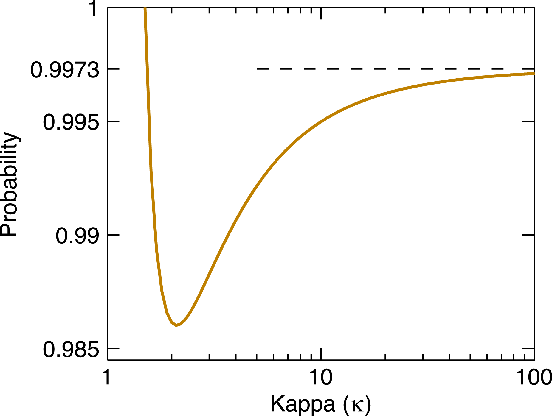
When ${\it\kappa}$ is not too close to $3/2$ , the standard deviation ${\it\sigma}_{{\it\kappa}}$ is approximately equal to the half-width at half-maximum (HWHM) of the distribution function (3.5). In particular, ${\it\sigma}_{{\it\kappa}}\approx$ HWHM for ${\it\kappa}\geqslant 2$ . Similar to the Gaussian distribution, approximately 99 % of the mass of the Kappa distribution (3.5) is contained in the velocity range $-3{\it\sigma}_{{\it\kappa}}<v-{\it\mu}<3{\it\sigma}_{{\it\kappa}}$ . The probability that $|v-{\it\mu}|<V$ is

(3.7) $$\begin{eqnarray}\text{Prob}(|v-{\it\mu}|<V)=I_{x}\left({\textstyle \frac{1}{2}},{\it\kappa}-{\textstyle \frac{1}{2}}\right),\end{eqnarray}$$

where $I_{x}(z,w)$ is the incomplete Beta function (Abramowitz & Stegun Reference Abramowitz and Stegun1972) with argument $x={\it\nu}^{2}/(1+{\it\nu}^{2})$ and ${\it\nu}^{2}=V^{2}/({\it\kappa}v_{0}^{2})$ . The graph of this probability shown in figure 1 demonstrates that $\text{Prob}(|v-{\it\mu}|<3{\it\sigma}_{{\it\kappa}})>98.6\,\%$ for all ${\it\kappa}>3/2$ .

Figure 1.

The probability that the particle velocity is contained in the interval $-3{\it\sigma}_{{\it\kappa}}<v-{\it\mu}<3{\it\sigma}_{{\it\kappa}}$ when the particle population follows the Kappa distribution (3.5). The dashed line is the corresponding probability for the Gaussian distribution with mean ${\it\mu}$ and standard deviation ${\it\sigma}$ . In the limit as ${\it\kappa}\rightarrow 3/2^{+}$ , ${\it\sigma}_{{\it\kappa}}\rightarrow \infty$ and the probability approaches unity.

4. Calculation of the kernel $D(k,{\it\tau})$ when ${\it\kappa}=n$

The Kappa distributions that yield analytically tractable solutions are generally those for which ${\it\kappa}=1,2,3,\dots \,$ . When ${\it\kappa}=n$ is a positive integer, the kernel (2.9) may be computed by means of the calculus of residues or a table of Fourier transforms. Substitution of the distribution function (3.5) into (2.9) yields

(4.1) $$\begin{eqnarray}D(k,{\it\tau})={\rm\pi}v_{0}^{2}A_{{\it\kappa}}{\it\omega}_{p}^{2}{\it\tau}\text{e}^{-\text{i}k{\it\mu}{\it\tau}}\int _{-\infty }^{\infty }\text{e}^{-\text{i}kv{\it\tau}}\left(1+\frac{v^{2}}{{\it\kappa}v_{0}^{2}}\right)^{-{\it\kappa}}\,\text{d}v\end{eqnarray}$$

or, equivalently,

(4.2) $$\begin{eqnarray}D(k,{\it\tau})={\rm\pi}v_{0}^{3}\sqrt{{\it\kappa}}A_{{\it\kappa}}{\it\omega}_{p}^{2}{\it\tau}\text{e}^{-\text{i}k{\it\mu}{\it\tau}}\int _{-\infty }^{\infty }\text{e}^{-\text{i}xy}(1+x^{2})^{-{\it\kappa}}\,\text{d}x,\end{eqnarray}$$

where $y=\sqrt{{\it\kappa}}v_{0}{\it\tau}k$ . When ${\it\kappa}=n$ is a positive integer, the remaining integral is evaluated using the calculus of residues or a table of Fourier transforms. For any real value of $y$ , that calculation yields

(4.3) $$\begin{eqnarray}\displaystyle & \displaystyle \int _{-\infty }^{\infty }\text{e}^{-\text{i}xy}(1+x^{2})^{-1}\,\text{d}x={\rm\pi}\exp (-|y|), & \displaystyle\end{eqnarray}$$

(4.4) $$\begin{eqnarray}\displaystyle & \displaystyle \int _{-\infty }^{\infty }\text{e}^{-\text{i}xy}(1+x^{2})^{-2}\,\text{d}x=\frac{{\rm\pi}}{2}(|y|+1)\exp (-|y|), & \displaystyle\end{eqnarray}$$

(4.5) $$\begin{eqnarray}\int _{-\infty }^{\infty }\text{e}^{-\text{i}xy}(1+x^{2})^{-3}\,\text{d}x=\frac{{\rm\pi}}{8}(y^{2}+3|y|+3)\exp (-|y|).\end{eqnarray}$$

Hence, when ${\it\kappa}=1$ , the kernel is

(4.6) $$\begin{eqnarray}D_{1}(k,{\it\tau})={\it\omega}_{p}^{2}{\it\tau}\exp (-\text{i}{\it\mu}{\it\tau}k-v_{e}{\it\tau}|k|),\end{eqnarray}$$

where $v_{e}=v_{0}$ . The variance of the distribution function is infinite in this case so, technically, the thermal speed is infinite. (An infinite second moment is unphysical since particle velocities never exceed the speed of light in vacuum, but only a relativistic treatment can properly take this into account.) In the case ${\it\kappa}=2$ , the kernel is

(4.7) $$\begin{eqnarray}D_{2}(k,{\it\tau})={\it\omega}_{p}^{2}{\it\tau}(1+v_{e}{\it\tau}|k|)\exp (-\text{i}{\it\mu}{\it\tau}k-v_{e}{\it\tau}|k|),\end{eqnarray}$$

where, from (3.6), the thermal speed is $v_{e}={\it\sigma}_{{\it\kappa}}=\sqrt{2}v_{0}$ . For integer values of ${\it\kappa}$ , the kernel is essentially an exponential function, which is especially convenient for the purpose of mathematical analysis.

The distribution function $f_{0}(v)={\it\delta}(v-{\it\mu})$ describes a cold plasma with a uniform flow velocity ${\it\mu}$ . The kernel in this case is, from (2.9),

(4.8) $$\begin{eqnarray}D(k,{\it\tau})={\it\omega}_{p}^{2}{\it\tau}\exp (-\text{i}{\it\mu}{\it\tau}k).\end{eqnarray}$$

The same result is obtained from (4.6) and (4.7) in the limit $v_{e}\rightarrow 0$ .

5. Derivation of the impulse response

The response of the plasma to a delta function impulse applied at $t=0$ is the Green’s function of the linearized one-dimensional Vlasov–Poisson equations, also called the impulse response. The Laplace transform of the integral equation (2.8) is obtained by the use of the convolution theorem, which yields

(5.1) $$\begin{eqnarray}\tilde{E}(k,s)=\frac{{\it\rho}_{0}}{\text{i}k{\it\varepsilon}_{0}}\frac{\text{e}^{-st_{0}}}{1+D(k,s)},\end{eqnarray}$$

where $s$ is the Laplace transform variable (Abramowitz & Stegun Reference Abramowitz and Stegun1972, Chapter 29). Here, $\tilde{E}(k,s)$ and $D(k,s)$ are the Laplace transforms of $\tilde{E}(k,t)$ and $D(k,t)$ , respectively, and the minor abuse of notation should not cause any confusion. Recall that if $G(s)$ is the Laplace transform of $g(t)$ and ${\it\tau}>0$ , then $\text{e}^{-s{\it\tau}}G(s)$ is the Laplace transform of $g(t-{\it\tau})u(t-{\it\tau})$ , where $u(t)=0$ for $t<0$ and $u(t)=1$ for $t>0$ . Therefore, the factor $\text{e}^{-st_{0}}$ in (5.1) causes a translation of the solution in the time domain and, since this translation is of no interest, it is expedient to now let $t_{0}\rightarrow 0^{+}$ and write

(5.2) $$\begin{eqnarray}\tilde{E}(k,s)=\frac{{\it\rho}_{0}}{\text{i}k{\it\varepsilon}_{0}}\frac{1}{1+D(k,s)}\end{eqnarray}$$

or, equivalently,

(5.3) $$\begin{eqnarray}\tilde{{\it\phi}}(k,s)=\frac{{\it\rho}_{0}}{k^{2}{\it\varepsilon}_{0}}\frac{1}{1+D(k,s)},\end{eqnarray}$$

where ${\it\phi}(x,t)$ is the electrostatic potential defined such that $E(x,t)=-\partial {\it\phi}/\partial x$ . Equations (5.2) and (5.3) are the solutions for the impulse response in the Laplace transform domain.

5.1. Impulse response when ${\it\kappa}=1$

The Laplace transform of the kernel $D_{1}$ in (4.6) is

(5.4) $$\begin{eqnarray}D_{1}(k,s)=\frac{{\it\omega}_{p}^{2}}{(s+a)^{2}},\quad a=\text{i}{\it\mu}k+v_{e}|k|.\end{eqnarray}$$

Hence, from (5.3), the impulse response is

(5.5) $$\begin{eqnarray}\tilde{{\it\phi}}(k,s)=\frac{{\it\rho}_{0}}{k^{2}{\it\varepsilon}_{0}}\frac{(s+a)^{2}}{(s+a)^{2}+{\it\omega}_{p}^{2}}.\end{eqnarray}$$

The inverse Laplace transform of this function is

(5.6) $$\begin{eqnarray}\tilde{{\it\phi}}(k,t)=\frac{{\it\rho}_{0}}{k^{2}{\it\varepsilon}_{0}}\exp (-at)[{\it\delta}(t)-{\it\omega}_{p}\sin ({\it\omega}_{p}t)].\end{eqnarray}$$

It follows that the plasma response vanishes in the limit as $t\rightarrow \infty$ . To find the solution, it only remains to calculate the inverse Fourier transform of $\tilde{{\it\phi}}(k,t)$ . The inverse Fourier transform of the function $k^{2}\tilde{{\it\phi}}(k,t)$ is

(5.7) $$\begin{eqnarray}\frac{\partial E(x,t)}{\partial x}=\frac{{\it\rho}_{0}}{{\rm\pi}{\it\varepsilon}_{0}}\frac{v_{e}t}{(x-{\it\mu}t)^{2}+(v_{e}t)^{2}}[{\it\delta}(t)-{\it\omega}_{p}\sin ({\it\omega}_{p}t)]\end{eqnarray}$$

and the inverse Fourier transform of the function $-\text{i}k\tilde{{\it\phi}}(k,t)$ is the electric field

(5.8) $$\begin{eqnarray}E(x,t)=\frac{{\it\rho}_{0}}{{\rm\pi}{\it\varepsilon}_{0}}\tan ^{-1}\left(\frac{x-{\it\mu}t}{v_{e}t}\right)[{\it\delta}(t)-{\it\omega}_{p}\sin ({\it\omega}_{p}t)].\end{eqnarray}$$

In the limit $v_{e}\rightarrow 0$ , this reduces to the cold plasma result derived from the kernel (4.8):

(5.9) $$\begin{eqnarray}E(x,t)=\frac{{\it\rho}_{0}}{2{\it\varepsilon}_{0}}\text{sgn}(x-{\it\mu}t)[{\it\delta}(t)-{\it\omega}_{p}\sin ({\it\omega}_{p}t)],\end{eqnarray}$$

where $\text{sgn}(x)=1$ if $x>0$ and $\text{sgn}(x)=-1$ if $x<0$ . Note that when the plasma bulk velocity vanishes, ${\it\mu}=0$ , the electric field is an odd function of $x$ , as required by symmetry. When ${\it\mu}\neq 0$ , the same symmetry holds with respect to the plane $x={\it\mu}t$ at time $t$ , the location of the original disturbance in the plasma frame. In other words, the electric field is an odd function of the argument $x-{\it\mu}t$ .

At any time $t>0$ , the electric field (5.8) approaches a constant as $|x|\rightarrow \infty$ . Moreover, the electric field everywhere in space is modulated by the common factor $\sin ({\it\omega}_{p}t)$ , which may be described as a ‘ringing’ of the plasma at the plasma frequency. The cause of this ringing phenomenon shall be explained in a moment. The factor $\tan ^{-1}[(x-{\it\mu}t)/v_{e}t]$ governs the spatial dependence of the electric field; it approaches ${\rm\pi}/2$ as $x\rightarrow \infty$ and $-{\rm\pi}/2$ as $x\rightarrow -\infty$ . For small times, the transition from $-{\rm\pi}/2$ to $+{\rm\pi}/2$ is localized near the point $x={\it\mu}t$ , where the field vanishes. As the time $t$ increases, the transition region becomes progressively wider with the result that $E(x,t)\rightarrow 0$ as $t\rightarrow \infty$ . 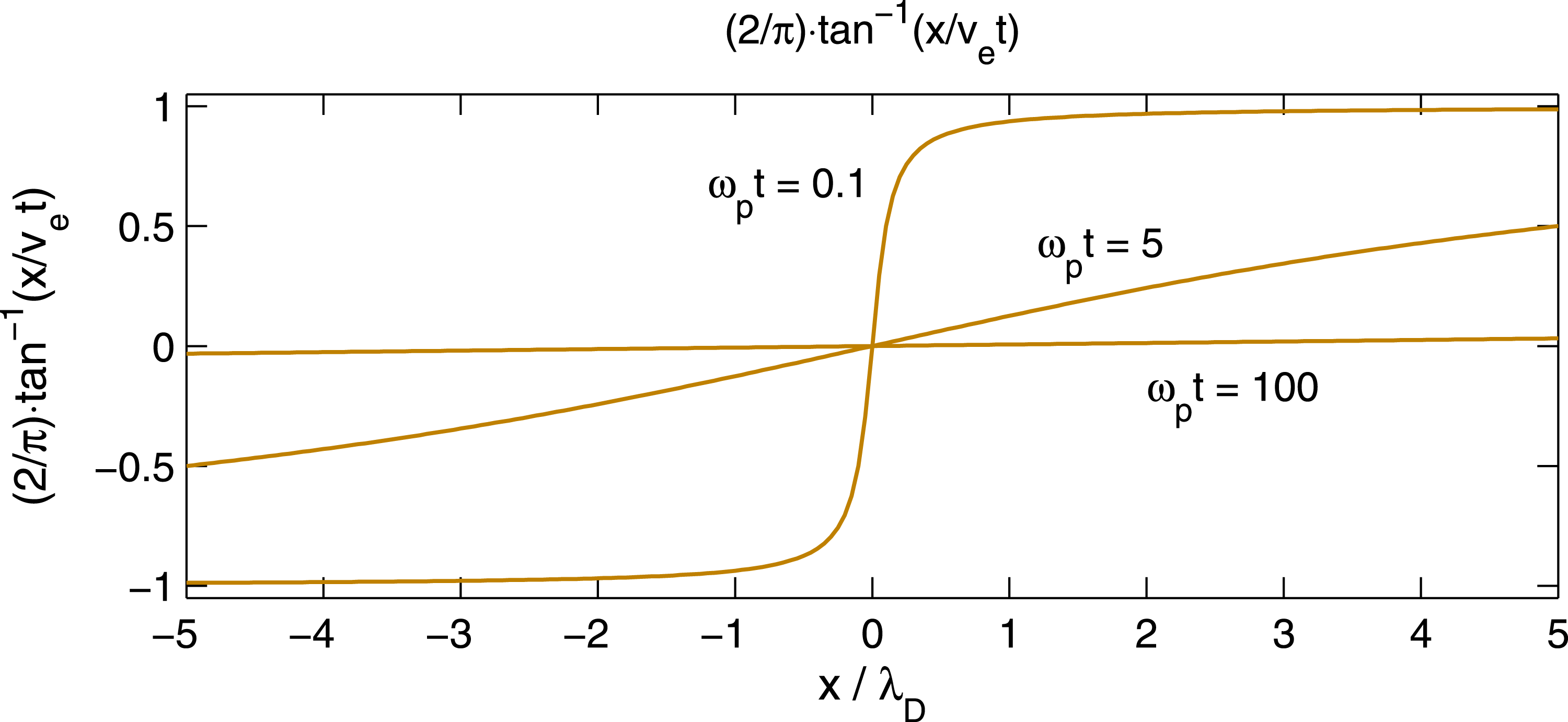This behaviour is sketched in figure 2. The half-width of the transition region at time $t$ , the point where the argument of the inverse tangent is unity, is ${\rm\Delta}x=v_{e}t$ or ${\rm\Delta}x/{\it\lambda}_{D}={\it\omega}_{p}t$ . Thus, the half-width of the transition region is equal to the distance travelled by a thermal electron in time $t$ .

Figure 2.

The factor $\tan ^{-1}[(x-{\it\mu}t)/v_{e}t]$ , which governs the spatial dependence of the electric field (5.8) in the case ${\it\kappa}=1$ , is plotted for ${\it\mu}=0$ at three different times: ${\it\omega}_{p}t=0.1$ , 5, and 100. Here, the Debye length is defined to be ${\it\lambda}_{D}=v_{e}/{\it\omega}_{p}$ .

The reason for the ringing at the plasma frequency may be explained as follows; see also Borovsky (Reference Borovsky1988) and Calder, Hulbert & Laframboise (Reference Calder, Hulbert and Laframboise1993). For simplicity, suppose that ${\it\mu}=0$ . In the absence of the plasma, a positive charge on the electrode, ${\it\rho}_{0}>0$ , generates a constant electric field $E(x)=({\it\rho}_{0}/2{\it\varepsilon}_{0})\text{sgn}(x)$ that points away from the electrode. In the limit as $t\rightarrow 0^{+}$ , the factor in front of the delta function in (5.8) is precisely equal to that same vacuum field. This vacuum field appears throughout the plasma for just an instant at $t=0$ , as is indicated by the delta function. It is this impulse at $t=0$ that sets the plasma into motion. The electrons respond by accelerating toward the electrode. As they do, a net negative charge builds up near the electrode causing an electric field that points toward the grid, represented by the term $\sin ({\it\omega}_{p}t)$ with a minus sign in (5.8). The field generated by the electrons eventually reverses the electron flow toward the grid and causes a flow away from the grid that soon results in a net positive charge at the location of the electrode. Then, the entire process repeats itself. This scenario results in electron plasma oscillations at the plasma frequency ${\it\omega}_{p}$ .

Corresponding to the electric field (5.8), the electrostatic potential which vanishes at $x={\it\mu}t$ is

(5.10) $$\begin{eqnarray}\displaystyle {\it\phi}(x,t) & = & \displaystyle -\frac{{\it\rho}_{0}v_{e}t}{{\rm\pi}{\it\varepsilon}_{0}}\left\{\frac{x-{\it\mu}t}{v_{e}t}\tan ^{-1}\left(\frac{x-{\it\mu}t}{v_{e}t}\right)-\frac{1}{2}\log \left[1+\left(\frac{x-{\it\mu}t}{v_{e}t}\right)^{2}\right]\right\}\nonumber\\ \displaystyle & & \displaystyle \times \,[{\it\delta}(t)-{\it\omega}_{p}\sin ({\it\omega}_{p}t)].\end{eqnarray}$$

This follows from the relation $\tan ^{-1}(x)=(\text{d}/\text{d}x)\{x\tan ^{-1}(x)-1/2\log (1+x^{2})\}$ . The potential grows asymptotically like ${\it\phi}(x,t)\sim x$ as $|x|\rightarrow \infty$ , consistent with the fact that the electric field (5.8) approaches a constant. This divergent behaviour is a consequence of the one-dimensional geometry of the problem.

The solution (5.8) has almost certainly appeared in the literature before. Unfortunately, I do not know who first published it nor do I know of specific references which show the explicit form given in (5.8). I would be grateful for any information concerning the appropriate references.

5.2. Impulse response when ${\it\kappa}=2$

The Laplace transform of the kernel $D_{2}$ in (4.7) is

(5.11) $$\begin{eqnarray}D_{2}(k,s)={\it\omega}_{p}^{2}\left[\frac{1}{(s+a)^{2}}+\frac{2v_{e}|k|}{(s+a)^{3}}\right],\end{eqnarray}$$

where $a=\text{i}{\it\mu}k+v_{e}|k|$ . It follows from (5.3) that the impulse response is

(5.12) $$\begin{eqnarray}\tilde{{\it\phi}}(k,s)=\frac{{\it\rho}_{0}}{k^{2}{\it\varepsilon}_{0}}\left\{1-\frac{{\it\omega}_{p}^{2}(s+a+2v_{e}|k|)}{(s+a)^{3}+{\it\omega}_{p}^{2}(s+a+2v_{e}|k|)}\right\}.\end{eqnarray}$$

To calculate the inverse Laplace transform, the roots of the denominator must be determined. The denominator may be written ${\it\omega}_{p}^{3}(z^{3}+z+2|k{\it\lambda}_{D}|)$ , where $z=(s+a)/{\it\omega}_{p}$ and ${\it\lambda}_{D}=v_{e}/{\it\omega}_{p}$ .

For any real number ${\it\alpha}$ , the polynomial equation $z^{3}+z+2{\it\alpha}=0$ has one real root and a pair of complex conjugate roots. The real root is $z_{0}=-(y_{2}-y_{1})$ and the complex conjugate roots are

(5.13) $$\begin{eqnarray}z^{\pm }=\frac{1}{2}(y_{2}-y_{1})\pm \frac{\text{i}\sqrt{3}}{2}(y_{2}+y_{1}),\end{eqnarray}$$

where

(5.14a,b ) $$\begin{eqnarray}y_{1}=\left(\sqrt{{\it\alpha}^{2}+{\it\beta}^{3}}-{\it\alpha}\right)^{1/3},\quad y_{2}=\left(\sqrt{{\it\alpha}^{2}+{\it\beta}^{3}}+{\it\alpha}\right)^{1/3},\end{eqnarray}$$

and ${\it\beta}=1/3$ (Abramowitz & Stegun Reference Abramowitz and Stegun1972, Chapter 3). For the problem at hand, ${\it\alpha}=|k{\it\lambda}_{D}|$ and

(5.15a,b ) $$\begin{eqnarray}y_{1}=\left(\sqrt{(k{\it\lambda}_{D})^{2}+(1/27)}-|k{\it\lambda}_{D}|\right)^{1/3},\quad y_{2}=\left(\sqrt{(k{\it\lambda}_{D})^{2}+(1/27)}+|k{\it\lambda}_{D}|\right)^{1/3}.\end{eqnarray}$$

The second term in the brackets on the right-hand side of (5.12) has the expansion

(5.16) $$\begin{eqnarray}\frac{z+2{\it\alpha}}{z^{3}+z+2{\it\alpha}}=\frac{A}{z-z^{+}}+\frac{B}{z-z^{-}}+\frac{C}{z-z_{0}},\end{eqnarray}$$

where, as before, $z=(s+a)/{\it\omega}_{p}$ and ${\it\alpha}=|k{\it\lambda}_{D}|$ . The expansion coefficients are

(5.17) $$\begin{eqnarray}\displaystyle & \displaystyle A=\frac{z^{+}+2{\it\alpha}}{(z^{+}-z_{0})(z^{+}-z^{-})}=-\frac{\text{i}}{3}\frac{(1+\text{i}\sqrt{3})y_{2}-(1-\text{i}\sqrt{3})y_{1}+4|k{\it\lambda}_{D}|}{(\sqrt{3}+\text{i})y_{2}^{2}-(\sqrt{3}-\text{i})y_{1}^{2}+(2\text{i}/3)}, & \displaystyle\end{eqnarray}$$

(5.18) $$\begin{eqnarray}\displaystyle & \displaystyle B=-\frac{z^{-}+2{\it\alpha}}{(z^{-}-z_{0})(z^{+}-z^{-})}=\frac{\text{i}}{3}\frac{(1-\text{i}\sqrt{3})y_{2}-(1+\text{i}\sqrt{3})y_{1}+4|k{\it\lambda}_{D}|}{(\sqrt{3}-\text{i})y_{2}^{2}-(\sqrt{3}+\text{i})y_{1}^{2}-(2\text{i}/3)}, & \displaystyle\end{eqnarray}$$

and

(5.19) $$\begin{eqnarray}C=\frac{z_{0}+2{\it\alpha}}{(z^{+}-z_{0})(z^{-}-z_{0})}=-\frac{(y_{2}-y_{1})-2{\it\alpha}}{3(y_{2}^{2}+y_{1}^{2})-1}.\end{eqnarray}$$

Furthermore, since $k$ is real, $B=A^{\ast }$ , that is, $B$ is the complex conjugate of $A$ . In terms of the original variables, the expansion (5.16) is

(5.20) $$\begin{eqnarray}\frac{z+2{\it\alpha}}{z^{3}+z+2{\it\alpha}}=\frac{{\it\omega}_{p}A}{s+a-{\it\omega}_{p}z^{+}}+\frac{{\it\omega}_{p}B}{s+a-{\it\omega}_{p}z^{-}}+\frac{{\it\omega}_{p}C}{s+a-{\it\omega}_{p}z_{0}},\end{eqnarray}$$

where the quantities $A$ , $B$ , $C$ , $z^{+}$ , $z^{-}$ , and $z_{0}$ depend on $k$ but not $s$ . The inverse Laplace transform of the last equation yields the solution

(5.21) $$\begin{eqnarray}\displaystyle \tilde{{\it\phi}}(k,t) & = & \displaystyle \frac{{\it\rho}_{0}}{k^{2}{\it\varepsilon}_{0}}\{\!{\it\delta}(t)-{\it\omega}_{p}A\exp \{-(a-{\it\omega}_{p}z^{+})t\}\nonumber\\ \displaystyle & & \displaystyle -\,{\it\omega}_{p}B\exp \{-(a-{\it\omega}_{p}z^{-})t\}-{\it\omega}_{p}C\exp \{-(a-{\it\omega}_{p}z_{0})t\}\!\},\end{eqnarray}$$

where $a=\text{i}{\it\mu}k+v_{e}|k|$ .

Several characteristic features of the solution (5.21) should be noted. First, when ${\it\mu}=0$ , the electric field is an odd function of $x$ . To show this, it is enough to note that (5.21) is an even function of $k$ , primarily because $y_{1}$ and $y_{2}$ in (5.15) are even functions, so that $\tilde{E}(k,t)=-\text{i}k\tilde{{\it\phi}}(k,t)$ is an odd function of $k$ . Second, if $E_{0}(x,t)$ is the solution for a plasma at rest, that is, for ${\it\mu}=0$ , then the solution for a uniformly flowing plasma is $E_{0}(x-{\it\mu}t,t)$ . In words, the electric field for a plasma moving with the uniform velocity ${\it\mu}$ is a rigid translation at the velocity ${\it\mu}$ of the solution of the electric field for a plasma at rest. This is because $\exp (-at)\exp (\text{i}kx)=\exp [\text{i}k(x-{\it\mu}t)]\exp (-v_{e}|k|t)$ .

On physical grounds, it is expected that the solution vanishes in the limit as $t\rightarrow \infty$ . It is easy to see that $z_{0}<0$ and, therefore, the last term in (5.21) vanishes as $t\rightarrow \infty$ . Furthermore,

(5.22) $$\begin{eqnarray}\text{Re}(a-{\it\omega}_{p}z^{+})=v_{e}|k|-\frac{{\it\omega}_{p}}{2}(y_{2}-y_{1})=\frac{{\it\omega}_{p}}{2}(z_{0}+2{\it\alpha})=\frac{{\it\omega}_{p}}{2}(-z_{0}^{3})>0,\end{eqnarray}$$

where ${\it\alpha}=|k{\it\lambda}_{D}|$ and, similarly, $\text{Re}(a-{\it\omega}_{p}z^{-})>0$ . This shows that the impulse response vanishes in the limit as $t\rightarrow \infty$ . The exponential functions in (5.21) also govern the rate of decay of the solution in Fourier space ( $k$ -space) since $A$ , $B$ , and $C$ are algebraic functions of $k$ .

By analogy with the solution (5.8) for ${\it\kappa}=1$ , it is reasonable to expect the solution (5.21) to exhibit ‘ringing’ at or near the plasma frequency. This is indeed the case. To see this, suppose that ${\it\mu}=0$ and note that for the term with coefficient $C$ in (5.21) the argument of the exponential is purely real (when ${\it\mu}=0$ ). Therefore, that term damps in time without any temporal oscillation. Only the terms with coefficients $A$ and $B$ can produce temporal oscillations because the argument ${\it\omega}_{p}z^{\pm }t$ contains a non-zero imaginary part. If $z^{\pm }=b\pm \text{i}c$ , then the first two terms on the right-hand side of (5.20) may be written

(5.23) $$\begin{eqnarray}\frac{A}{s+a-{\it\omega}_{p}(b+\text{i}c)}+\frac{A^{\ast }}{s+a-{\it\omega}_{p}(b-\text{i}c)},\end{eqnarray}$$

where $a$ , $b$ , and $c$ are purely real when ${\it\mu}=0$ . The last expression is equivalent to

(5.24) $$\begin{eqnarray}(A+A^{\ast })\frac{s+a-{\it\omega}_{p}b}{(s+a-{\it\omega}_{p}b)^{2}+({\it\omega}_{p}c)^{2}}+\text{i}(A-A^{\ast })\frac{{\it\omega}_{p}c}{(s+a-{\it\omega}_{p}b)^{2}+({\it\omega}_{p}c)^{2}},\end{eqnarray}$$

which has the inverse Laplace transform

(5.25) $$\begin{eqnarray}\{(A+A^{\ast })\cos ({\it\omega}_{p}ct)+\text{i}(A-A^{\ast })\sin ({\it\omega}_{p}ct)\}\exp [-(a-{\it\omega}_{p}b)t].\end{eqnarray}$$

Hence, the solution (5.21) is equivalent to

(5.26) $$\begin{eqnarray}\displaystyle \tilde{{\it\phi}}(k,t) & = & \displaystyle \frac{{\it\rho}_{0}}{k^{2}{\it\varepsilon}_{0}}\{\!{\it\delta}(t)-{\it\omega}_{p}(A+A^{\ast })\cos ({\it\omega}_{p}ct)\exp [-(a-{\it\omega}_{p}b)t]\nonumber\\ \displaystyle & & \displaystyle -\,{\it\omega}_{p}\text{i}(A-A^{\ast })\sin ({\it\omega}_{p}ct)\exp [-(a-{\it\omega}_{p}b)t]-{\it\omega}_{p}C\exp \{-(a+2{\it\omega}_{p}b)t\}\!\},\nonumber\\ \displaystyle & & \displaystyle\end{eqnarray}$$

where $a=\text{i}{\it\mu}k+v_{e}|k|$ , $b=\text{Re}(z^{+})$ , and $c=\text{Im}(z^{+})$ .

Because $c=\text{Im}(z^{+})$ depends on $k$ , see (5.13) and (5.15), the temporal frequency ${\it\omega}(k)={\it\omega}_{p}c$ now depends on $k$ . In this respect, the solution in the case ${\it\kappa}=2$ is different from that in the case ${\it\kappa}=1$ , where the frequency of the ‘ringing’ is independent of wavenumber. However, because the dependence of the frequency ${\it\omega}(k)={\it\omega}_{p}c$ on $k$ is very weak, this mild wavenumber dependence is not expected to significantly alter the ringing phenomenon. Note that $c=\text{Im}(z^{+})\approx 1$ for $|k{\it\lambda}_{D}|\ll 1$ and $c$ increases very slowly since $c=\text{Im}(z^{+})\approx (2|k{\it\lambda}_{D}|)^{1/3}$ for $|k{\it\lambda}_{D}|\gg 1$ . Therefore, because Langmuir waves are strongly damped for $k{\it\lambda}_{D}\gtrsim 1$ , it is logical to expect that the frequency of the ringing is approximately independent of wavenumber and $c=\text{Im}(z^{+})\approx 1$ is a reasonable approximation.

Unfortunately, it does not appear to be possible to carry out the inverse Fourier transform of the solution (5.21) analytically. Nevertheless, the inverse Fourier transform may be calculated numerically with high precision.

6. Numerical calculation of the inverse Fourier transform

The numerical calculation of the inverse Fourier transform is accomplished using the fast Fourier transform (FFT) algorithm. Even though there is nothing novel about the numerical scheme, no reference covers the precise procedure used here, which may be described as follows. Suppose that it is required to compute the inverse Fourier transform $f(x)$ of the function $F(k)$ . And, suppose that the function $F(k)$ vanishes outside the interval $|k|\leqslant B$ , that is, the function $F(k)$ is band-limited with bandwidth $B$ . Then

(6.1) $$\begin{eqnarray}f(x)=\frac{1}{2{\rm\pi}}\int _{-B}^{B}F(k)\exp (\text{i}kx)\,\text{d}k.\end{eqnarray}$$

In practice, if $F(k)$ is not band-limited, then the inversion integral must be truncated and the truncation point $B$ chosen so that the mean square energy contained outside the interval $-B\leqslant k\leqslant B$ is negligible. The truncation point $B$ may be adjusted, if necessary, to ensure that the numerical solution is as accurate as required.

The integral (6.1) is approximated by a Riemann sum of the form

(6.2) $$\begin{eqnarray}\frac{1}{2{\rm\pi}}\int _{-B}^{B}F(k)\exp (\text{i}kx)\,\text{d}k\approx \frac{1}{2{\rm\pi}}\mathop{\sum }_{n=0}^{N-1}F(k_{n}^{\,\prime })\exp (\text{i}k_{n}^{\,\prime }x){\rm\Delta}k,\end{eqnarray}$$

where $k_{n}^{\,\prime }=(k_{n}+k_{n+1})/2$ , $k_{n}=-B+n{\rm\Delta}k$ for $n=0,1,2,\dots ,N$ , and ${\rm\Delta}k=2B/N$ . Here, $N$ may be any positive integer, but it is usually a good idea to let $N$ be an even integer to avoid having to evaluate the function $F(k)$ at the point $k=0$ , which may diverge, for example, if $F(k)=\exp (-|k|)/(\text{i}k)$ . Therefore, $N$ is a positive even integer in what follows.

The Riemann sum (6.2) is based on the midpoint rule and, in that case, it is an established result of the calculus that whenever $F(k)$ and its first derivative $F^{\prime }(k)$ are both continuously differentiable functions for $-B\leqslant k\leqslant B$ , the Riemann sum converges to the integral on the left-hand side with an absolute error proportional to $({\rm\Delta}k)^{2}$ as ${\rm\Delta}k\rightarrow 0$ . Convergence still occurs when the preceding conditions hold piecewise on the interval $-B\leqslant k\leqslant B$ , but the convergence rate may be less than second order in that case. It remains to show how the Riemann sum (6.2) may be computed using the FFT.

From the preceding definitions, it follows that $k_{n}^{\,\prime }=-B+(n+1/2){\rm\Delta}k$ and, with that substitution, the Riemann sum in (6.2) becomes

(6.3) $$\begin{eqnarray}\frac{1}{2{\rm\pi}}\exp \left\{-\text{i}Bx\left(1-\frac{1}{N}\right)\right\}\mathop{\sum }_{n=0}^{N-1}F(k_{n}^{\,\prime })\exp \left(\frac{\text{i}2Bnx}{N}\right){\rm\Delta}k.\end{eqnarray}$$

This expression is evaluated at the Fourier nodes $x_{m}=m{\rm\pi}/B$ , where $|m|\leqslant N/2$ , to obtain

(6.4) $$\begin{eqnarray}\frac{1}{2{\rm\pi}}\exp \left\{-\text{i}{\rm\pi}m\left(1-\frac{1}{N}\right)\right\}\mathop{\sum }_{n=0}^{N-1}F(k_{n}^{\,\prime })\exp \left(\frac{2{\rm\pi}\text{i}nm}{N}\right){\rm\Delta}k.\end{eqnarray}$$

The sum on the right-hand side is now in the standard form of the inverse FFT of the ordered sequence $(F_{0},F_{1},F_{2},\dots ,F_{N-1})$ , where $F_{n}=F(k_{n}^{\,\prime })$ . Let $\boldsymbol{Q}(m)$ denote the inverse FFT

(6.5) $$\begin{eqnarray}\boldsymbol{Q}(m)=\mathop{\sum }_{n=0}^{N-1}F(k_{n}^{\,\prime })\exp \left(\frac{2{\rm\pi}\text{i}nm}{N}\right),\end{eqnarray}$$

where $m=0,1,2,\dots ,N-1$ . Note that there is no prefactor $1/N$ in the definition of the inverse FFT used here. Thus, the Riemann sum, (6.4), may be written

(6.6) $$\begin{eqnarray}R_{m}=\frac{B}{N{\rm\pi}}\exp \left\{-\text{i}{\rm\pi}m\left(1-\frac{1}{N}\right)\right\}\boldsymbol{Q}(m).\end{eqnarray}$$

So far, $\boldsymbol{Q}(m)$ has been defined by (6.5) for $0\leqslant m<N$ , but it is required to determine $R_{m}$ in (6.6) for $-N/2\leqslant m\leqslant N/2$ . Therefore, it is necessary to evaluate $\boldsymbol{Q}(m)$ for $m<0$ . The FFT is cyclic, that is, $\boldsymbol{Q}(-N+m)=\boldsymbol{Q}(m)$ and, therefore,

(6.7) $$\begin{eqnarray}\displaystyle & & \displaystyle \{\boldsymbol{Q}(-N/2),\boldsymbol{Q}[-(N/2)+1],\boldsymbol{Q}[-(N/2)+2],\dots ,\boldsymbol{Q}(-1)\}\nonumber\\ \displaystyle & & \displaystyle \quad =\{\boldsymbol{Q}(N/2),\boldsymbol{Q}[(N/2)+1],\boldsymbol{Q}[(N/2)+2],\dots ,\boldsymbol{Q}(N-1)\}.\end{eqnarray}$$

These relations are used to calculate $\boldsymbol{Q}(m)$ in (6.6) for $-N/2\leqslant m<0$ . Thus, $R_{m}$ in (6.6) is well defined for all indices $-N/2\leqslant m\leqslant N/2$ . The inverse Fourier transform of the function $F(k)$ is thus approximated by $f(x_{m})\approx R_{m}$ , where $x_{m}=m{\rm\pi}/B$ and $-N/2\leqslant m\leqslant N/2$ . The accuracy of this numerical approximation may be improved by increasing $N$ and, if necessary, the spatial resolution may be refined by increasing  $B$ .

The procedure may be summarized as follows. Step (i): Compute $\boldsymbol{Q}(m)$ as the inverse FFT of the sequence $(F_{0},F_{1},F_{2},\dots ,F_{N-1})$ , where $F_{n}=F(k_{n}^{\,\prime })$ . Step (ii): Rearrange the vector $\boldsymbol{Q}$ to obtain $\{\boldsymbol{Q}(-N/2),\dots ,\boldsymbol{Q}(-1),\boldsymbol{Q}(0),\boldsymbol{Q}(1),\dots ,\boldsymbol{Q}(N/2)\}$ . Step (iii): Multiply $\boldsymbol{Q}(m)$ by the factor shown in (6.6). Step (iv): Increase $N$ and repeat steps (i)–(iii) until the desired accuracy is achieved and, if necessary, increase $B$ to refine the spatial resolution ${\rm\Delta}x={\rm\pi}/B$ .

7. Results for the case ${\it\kappa}=2$

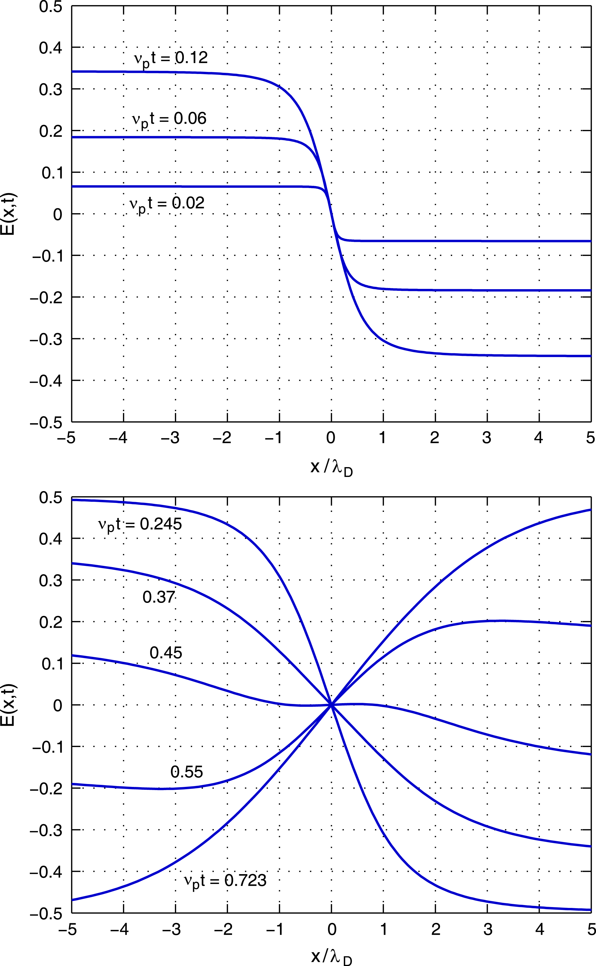
The inverse Fourier transform of the electric field $\tilde{E}(k,t)=-\text{i}k\tilde{{\it\phi}}(k,t)$ in (5.21) or (5.26) may be accurately calculated for any $t>0$ using the procedure described in the previous section. Sample results are shown in figure 3 for the case when the mean velocity is zero: ${\it\mu}=0$ . When ${\it\mu}\neq 0$ , the electric field at time $t$ is obtained by moving the field shown in figure 3 by a distance $d={\it\mu}t$ . For small values of ${\it\nu}_{p}t=({\it\omega}_{p}t)/2{\rm\pi}$ , the electric field in figure 3 consists of an abrupt change in sign near the origin that resembles a discontinuity. The field amplitude on the left-hand side of the discontinuity grows as time increases and the width of the transition region near the origin increases with time. The amplitude on the left-hand side, $x<0$ , eventually reaches a local maximum around ${\it\nu}_{p}t=0.245$ at which time the amplitude starts to decrease, reaching a minimum around ${\it\nu}_{p}t=0.723$ . Thereafter, the amplitude oscillates in time with a frequency near the plasma frequency ${\it\nu}_{p}$ . The behaviour of the solution for ${\it\kappa}=2$ is qualitatively similar to that for ${\it\kappa}=1$ given by (5.8).

Figure 3.

The electric field $E(x,t)$ of a Langmuir pulse triggered at $t=0$ in a plasma characterized by a Kappa distribution with ${\it\kappa}=2$ and mean velocity ${\it\mu}=0$ . The electric field is an odd function of $x$ shown at different times marked in the figure. The leading coefficient of the electric field has been set to unity, that is, ${\it\rho}_{0}{\it\omega}_{p}/{\it\varepsilon}_{0}=1$ .

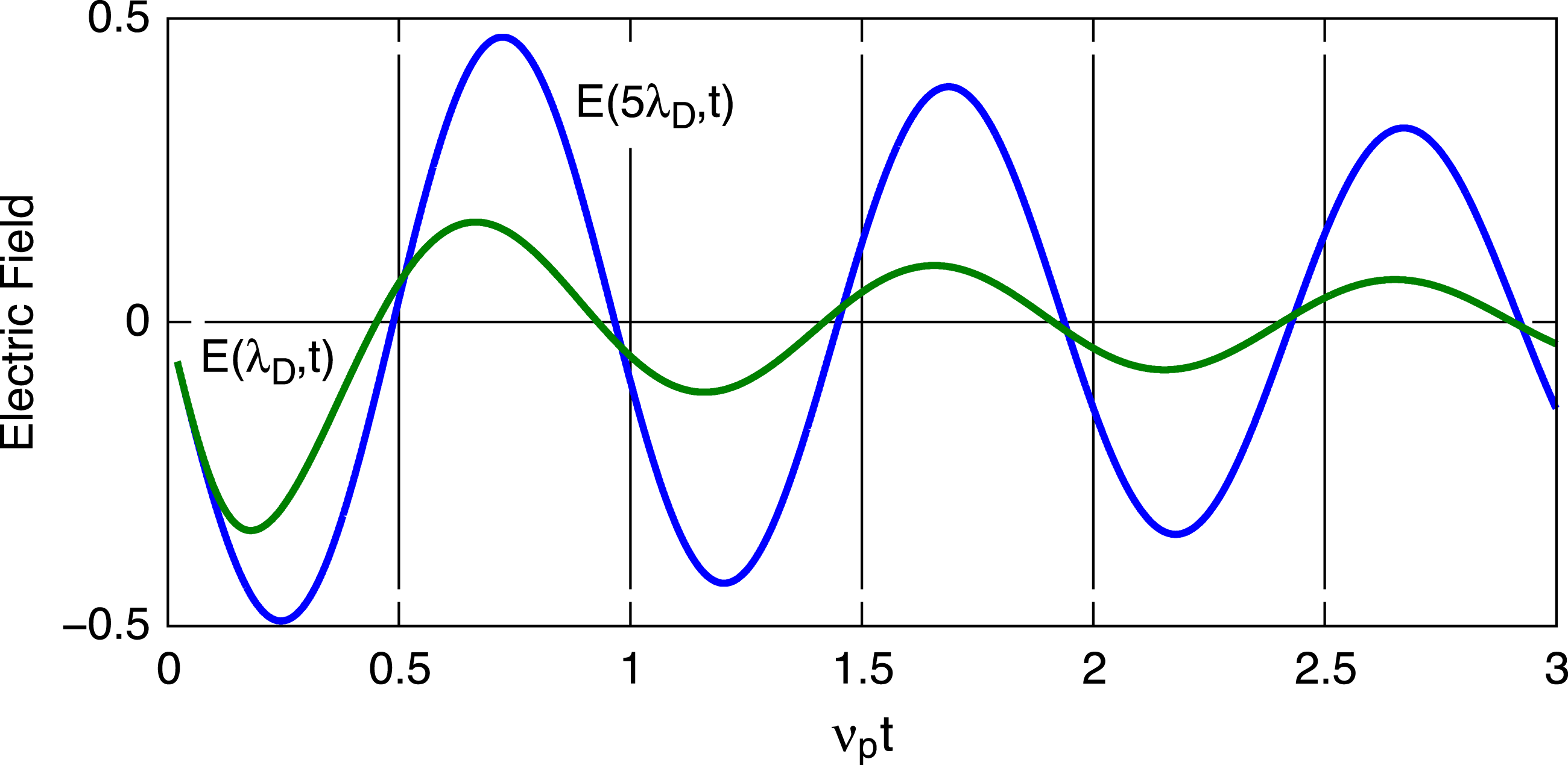
The electric field at any fixed point in space $x\neq 0$ behaves like a damped sinusoid. Examples of the electric field as a function of time at the points $x={\it\lambda}_{D}$ and $x=5{\it\lambda}_{D}$ are shown in figure 4. Close inspection of figure 4 reveals that the period of oscillation is less than the plasma period $1/{\it\nu}_{p}$ . An examination of the zero crossings for $t>0$ shows that the spacings of the successive zero crossings shown in figure 4, not including the origin, are ${\it\nu}_{p}{\rm\Delta}t\approx 0.478$ , 0.490, 0.493, 0.496, and 0.497 for the waveform at $x={\it\lambda}_{D}$ and ${\it\nu}_{p}{\rm\Delta}t\approx 0.479$ , 0.483, 0.488, 0.492, and 0.493 for the waveform at $x=5{\it\lambda}_{D}$ . These results tentatively suggest that at any point $x\neq 0$ , the frequency of oscillation approaches ${\it\nu}_{p}$ asymptotically as $t\rightarrow \infty$ . This behaviour is quite different from the solution for ${\it\kappa}=1$ in which the waveform at any point $x$ oscillates like $\sin ({\it\omega}_{p}t)$ for all $t>0$ .

Figure 4.

The electric field $E(x,t)$ as a function of time at the points $x={\it\lambda}_{D}$ (green) and $x=5{\it\lambda}_{D}$ (blue). The two curves may be distinguished by the fact that the field at $x=5{\it\lambda}_{D}$ has a greater peak amplitude than the field at $x={\it\lambda}_{D}$ . The plasma is characterized by a Kappa distribution with ${\it\kappa}=2$ and mean velocity ${\it\mu}=0$ . The leading coefficient of the electric field has been set to unity so that ${\it\rho}_{0}{\it\omega}_{p}/{\it\varepsilon}_{0}=1$ .

The source of this interesting behaviour is the wavenumber dependence of the frequency in (5.26), where ${\it\omega}(k)/{\it\omega}_{p}=(\sqrt{3}/2)(y_{2}+y_{1})$ with the functions $y_{1}(k)$ and $y_{2}(k)$ given by (5.15). As $t\rightarrow \infty$ , the function $\tilde{E}(k,t)=-\text{i}k\tilde{{\it\phi}}(k,t)$ in (5.26) becomes progressively more localized near the origin $k=0$ where the approximation ${\it\omega}(k)\approx {\it\omega}_{p}$ holds for $|k{\it\lambda}_{D}|\ll 1$ . This explains why the oscillation frequency of the waveform at a fixed point $x$ approaches ${\it\nu}_{p}$ as $t\rightarrow \infty$ . Even though this behaviour is understood, it is of practical interest to develop an approximation of $E(x,t)$ that incorporates this behaviour, such as $E(x,t)\approx A\sin ({\it\omega}t+{\it\varphi})$ , where $A$ , ${\it\omega}$ , and ${\it\phi}$ are slowly varying and may depend on $x$ and $t$ . Unfortunately, the method of stationary phase does not produce such an approximation.

8. Application to the solar wind

The properties of the impulse response of an ideal grid electrode suggest a simple way of using small-amplitude Langmuir pulses to measure the bulk flow velocity of nearly collisionless plasmas such as the solar wind. Suppose that a low-power transmitter and a receiver are connected to two parallel-plate electrodes separated by a distance $d=1~\text{m}$ . As a practical matter, two point probes would probably be used rather than planar electrodes. Distances on the order of 1 m or less are generally reasonable for spacecraft instrumentation. Suppose that a Langmuir pulse is triggered on the upstream electrode at time $t$ . According to the solutions (5.8) and (5.26), the electric field at the downstream electrode exhibits a ringing at the plasma frequency ${\it\nu}_{p}={\it\omega}_{p}/2{\rm\pi}$ that undergoes an abrupt $180^{\circ }$ phase change at time $t+{\it\tau}$ , where ${\it\tau}=d/{\it\mu}$ . By detecting the time when this phase shift occurs, the plasma bulk velocity ${\it\mu}=d/{\it\tau}$ may be measured. For a bulk speed ${\it\mu}=500~\text{km}~\text{s}^{-1}$ and $d=1~\text{m}$ , the time delay is ${\it\tau}=2~{\rm\mu}\text{s}$ . Because time delays may be measured electronically with high precision, this method may provide a way to measure plasma bulk velocities with high accuracy.

A typical value of the plasma frequency in the solar wind is ${\it\nu}_{p}\approx 25~\text{kHz}$ . Therefore, a delay of ${\it\tau}=2~{\rm\mu}\text{s}$ implies ${\it\omega}_{p}{\it\tau}\approx 0.3$ and, as can be seen in figure 2, for such small values of ${\it\omega}_{p}{\it\tau}$ the spatial dependence of the electric field is characterized by an abrupt transition that is not yet ‘smeared out’. Whenever ${\it\omega}_{p}{\it\tau}\ll 1$ , the spatial dependence of the electric field exhibits a relatively rapid change in sign as a function of position in the neighbourhood of the point $x={\it\mu}{\it\tau}$ . A rapid transition is important in applications because it allows an accurate measurement of the time when the phase change occurs. Considering that the voltage applied to the electrode is only an approximation of a delta function in time ${\it\delta}(t)$ , the implementation of this measurement technique in the solar wind requires that the voltage pulse applied to the electrode must have a rise time that is much smaller than the plasma period $1/{\it\nu}_{p}$ and, moreover, much smaller than ${\it\tau}$ .

The measurement technique just described is based on the fact that the pulse or ‘discontinuity’ in the electric field propagates with the plasma bulk speed ${\it\mu}$ . It is noteworthy that this property is independent of the value of ${\it\kappa}$ and, therefore, the conclusions of this study are not restricted to plasmas with ${\it\kappa}=1$ or ${\it\kappa}=2$ . Even though there are many engineering details that remain to be worked out, this study clearly demonstrates that the basic principle of the measurement technique is scientifically sound. If the engineering is viable, this technique should enable measurements of the solar wind bulk velocity that are faster, more accurate, and more cost effective than established techniques that employ electrostatic analysers and Faraday cups.