1. Introduction
1.1. In Part 1 of this series of papers (Wilkie et al., Reference Wilkie, Şahin, Cairns and Kleinow2011), we updated the parameters of the Wilkie model to 2009, slightly modifying some parts of the model. We now have available 5 more years of June data, and we start in section 2 by considering how the model has fared in this period. We then in section 3 discuss the variables that can form the working set, the input set and the output set for a simulation, all of which may be different. There are different ways of simulating, either in a linear parallel structure or in a branching tree structure.
1.2. In section 4, we discuss the initial conditions required, which may be market conditions at some date, or may be “neutral” initial conditions, which may be defined in different ways, and are discussed in sections 5 and 6. In section 6 and Appendix, we give the long-term means, variances and covariances of the variables and initial condition. What we call “neutralising parameters” may have a role, and in section 7 we discuss how these may be derived. Finally, in section 8 we suggest using additional information in the first periods of the simulation to adjust the formulae or parameters for a limited “select period”. Although we are mainly discussing the Wilkie model, many of the aspects apply to any similar model used for simulation over time.
2. The Model and the Experience Since 2009
2.1. It is convenient to start by repeating, with minimum explanation, the formulae for the model and the parameter values suggested in 2009. The variables considered at any time t are:
Q(t) a retail prices index (or some other index of consumer prices)
I(t)=lnQ(t)−lnQ(t−1) the annual rate of price inflation
W(t) an index of personal earnings or wages
J(t)=lnW(t)−lnW(t−1) the annual rate of wage inflation
P(t) a price index of ordinary shares, calculated as D(t)/Y(t)
Y(t) the dividend yield on an index of ordinary shares
D(t) the corresponding dividend index=P(t)×Y(t)
K(t)=lnD(t)−lnD(t−1) the annual rate of dividend increase
C(t) an indicator of long-term yields on government stock
B(t) an indicator of short-term interest rates
R(t) an indicator of real yields on index-linked stocks
Note that although rates such as Y(t), C(t), B(t) and R(t) are often popularly expressed as percentages per year and have varying frequencies of compounding, we process them always per unit as decimal fractions, as we do with I(t), J(t) and K(t), which, however, are continuously compounded annual rates.
2.2. For any variable modelled, denoted X, the following holds, except where especially noted in section 8:
 $$XE(t)=XSD.XZ(t)$$
where XZ(t) has zero mean and unit standard deviation. We have generally assumed that each XZ(t) is unit normal, but the residuals are in many cases clearly not normally distributed; we intend to discuss this point further in a later part of this series.
For several variables we use XN(t)=X(t)−XMU, so that each XN has zero mean. We also use a suffix L to denote the logarithm of a variable, so we use QL(t)=lnQ(t), WL(t)=lnW(t), etc.; we use this also for certain parameters, so YMUL=lnYMU, etc.
2.3. The basic formulae, expressed in a sequence for simulation, are, for inflation, Q(t):
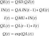 $$\eqalignno{ QE(t)&=QSD.QZ(t) \cr IN(t)&=QA.IN(t{\minus}{\rm 1}){\plus}QE(t) \cr I(t)&=QMU{\plus}IN(t) \cr QL({t})&=QL(t{\minus}{\rm 1}){\plus}I(t) \cr Q(t)&={\rm exp(}QL(t){\rm )} $$
Parameters suggested in Part 1 were:
 $$QMU=0.0{\rm 43};\,QA=0.{\rm 58};\,QSD=0.0{\rm 4}$$
2.4. For wages, W(t):
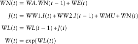 $$\eqalignno{ WN(t)& =WA.WN(t-{\rm 1}){\plus}WE(t) \cr J(t)& =WW{\rm 1}.I(t){\plus}WW{\rm 2}.I(t-{\rm 1}){\plus}WMU{\plus}WN(t) \cr WL(t)& =WL(t-{\rm 1}){\plus}J(t) \cr W(t)& ={\rm exp(}WL(t){\rm )} $$
Parameters suggested in Part 1 were:
 $$WA=0,\,WW{\rm 1}=0.{\rm 6}0;\,WW{\rm 2}=0.{\rm 27};\,WMU=0.0{\rm 2}0;\,WSD=0.0{\rm 219}$$
As the model seems satisfactory with WA=0, we could omit WN(t) entirely, but it does also seem possible that WA might have a use at a later period or in another economy, so it could be retained.
2.5. For share dividend yields, Y(t):
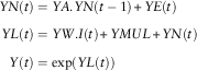 $$\eqalignno{ YN(t)& =YA.YN(t-{\rm 1}){\plus}YE(t) \cr YL(t)& =YW.I(t){\plus}YMUL{\plus}YN(t) \cr Y(t)& ={\rm exp(}YL(t){\rm )} $$
Parameters suggested in Part 1 were:
 $$\eqalignno{ YW= \,& {\rm 1}.{\rm 55};\,YMU=0.0{\rm 375};\,YA=0.{\rm 63};\,YSD=0.{\rm 155} \cr YMUL =&-\!{\rm 3}.{\rm 283414} $$
2.6. For the share dividend index, D(t):
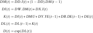 $$\eqalignno{ DM(t)& =DD.I(t){\plus}({\rm 1}-DD).DM(t-{\rm 1}) \cr DI(t)& =DW.DM(t){\plus}DX.I(t) \cr K(t)& =DI(t){\plus}DMU{\plus}DY.YE(t{\minus}1){\plus}DB.DE(t{\minus}1){\plus}DE(t) \cr DL(t)&=DL(t{\minus}1){\plus}K(t) \cr D(t)& ={\rm exp(}DL(t){\rm )} $$
Parameters suggested in Part 1 were:
 $$\eqalignno{ DW&=0.{\rm 43};\,DD=0.{\rm 16};\,DX={\rm 1}-DW=0.{\rm 57};\,DMU=0.0{\rm 11};\,DY=-0.{\rm 22}; \cr DB& =0.{\rm 43};\,DSD=0.0{\rm 7} $$
The share price index, P(t), can be calculated as D(t)/Y(t) or by PL(t)=DL(t)−YL(t).
2.7. For long-term interest rates, C(t):
 $$\eqalignno{ CN(t)& =CA.CN(t{\minus}1){\plus}CY.YE(t){\plus}CE(t) \cr CRL(t)& =CMUL{\plus}CN(t) \cr CR(t)& ={\rm exp(}CRL(t){\rm )} \cr CM(t)& ={\rm Max(}CD.I(t){\plus}({\rm 1}-CD).CM(t-{\rm 1}),CMIN{\minus}CR(t){\rm )} \cr C(t)&=CR(t){\plus}CM(t) $$
Parameters suggested in Part 1 were:
 $$\eqalignno{ & CD=0.0{\rm 45};\,CW={\rm 1};\,CMU={\rm 2}.{\rm 23}\,\%\,;\,CA=0.{\rm 92};\,CY=0.{\rm 37};\,CSD=0.{\rm 255} \cr & CMUL=-{\rm 3}.{\rm 8}0{\rm 3169} $$
Note that the constraint on CM(t) has to be applied differently when looking backwards than when looking forwards. When processing past data, the values of C(t) are given. CM(t) is our estimate of the market’s estimate of future inflation rates, based on an exponentially weighted moving average of past inflation rates. CM(t) is deducted from C(t) to give the implied “real” rate, CR(t). If CM(t) is bigger than C(t), then the calculated value of CR(t) becomes negative. As we wish to model lnCR(t), a negative value for CR(t) is undesirable. So, for the past, we reduce the value of CM(t) in any year so that C(t)−CM(t) is no smaller than some minimum value, denoted CMIN, which we set at 0.005 or 0.5%. Thus, for analysing past data we have (as given in Part 1):
 $$CM(t)={\rm Min(}CD.I(t){\plus}({\rm 1}-CD).CM(t-{\rm 1}),\,C(t)-CMIN{\rm )}$$
For future simulation, CR(t) is calculated so that it cannot be negative, but if CM(t) were to be negative to too great an extent, which is possible in the simulations, though it has not happened in the past data period we have used, then the calculated value of C(t)=CM(t)+CR(t) might be negative. This also is undesirable, so we would increase CM(t) so that C(t) is no less than some minimum, also called CMIN, and also set at set 0.005 or 0.5%. Thus, for the future, the formula for CM(t) is:
 $$CM(t)={\rm Max}\,{\rm (}CD.I(t){\plus}({\rm 1}-CD).CM(t-{\rm 1}),\,CMIN{\minus}CR(t){\rm )}$$
Strictly, this is a different constraint from the first one, and the values of CMIN could be different, so perhaps we should call them CMIN1 and CMIN2. In practice there is no confusion.
In both cases we have chosen to alter the value of CM(t) to be carried forward; one alternative would have been to alter the value of CR(t) and carry the altered value forward; another would have been to adjust the values of CR(t) or C(t) as appropriate without altering the carried forward values of CM(t) and CR(t). We consider that our choice is the best of these. We are sorry that all this was not made clear in Part 1, where only part of the story was explained.
2.8. For short-term interest rates, B(t):
 $$\hskip -64pt\eqalignno{ BN(t)& =BA.BN(t-{\rm 1}){\plus}BE(t) \cr BD(t)& =BMU{\plus}BN(t) \cr B(t)& =C(t).{\rm exp(}\!\!-\!\!BD(t){\rm )} $$
Parameters suggested in Part 1 were:
 $$BMU=0.{\rm 17};\,BA=0.{\rm 73};\,BSD=0.{\rm 3}$$
2.9. For “real” interest rates on index-linked stocks, R(t):
 $$\eqalignno{ RN(t)& =RA.RN(t{\minus}1){\plus}RBC.CE(t){\plus}RE(t) \cr R(t)&=RMU{\plus}RN(t) $$
Parameters suggested in Part 1 were (see Corrigenda):
 $$RMU={\rm 3}\,\%\,;\,RA=0.{\rm 95};\,RBC=0.00{\rm 8};\,RSD=0.00{\rm 3}$$
2.10. In Part 1, we showed how to calculate one-step-ahead forecasts for each year on the basis of the previous year, and also multi-step forecasts, in which forecasts for future years are calculated on the basis of the experience up to some intermediate year. In this case we can calculate forecast one-step-ahead values for 2010–2014, each on the basis of the data for the previous year and the data for previous series in the same year, and also forecast multi-step values for these years, all on the basis of the data only up to 2009. In each case the forecast values can be compared with the actual experience to see how well the model is behaving relatively to the actual data. We have made these comparisons. We do not give full details of them all, but we summarise them below.
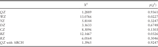
2.11. The one-step-ahead forecasts for I(t), Y(t), K(t), C(t), R(t) and I(t) with the ARCH model show nothing surprising. We compare the differences between the observed figures for each year and those expected by the model, QE(t), etc., each divided by the corresponding standard deviations, QSD, etc., giving values of QZ(t), etc. These differences should be distributed as unit normal, so the sums of their squares, which we denote X 2, should be distributed as χ 2 with 5 d.f. In Table 1 we show these values, along with the corresponding probabilities, the p-values from the χ 2 test.
Values of X 2 and probabilities from a χ 2 test for one-step-ahead forecasts from 2009 to 2014.
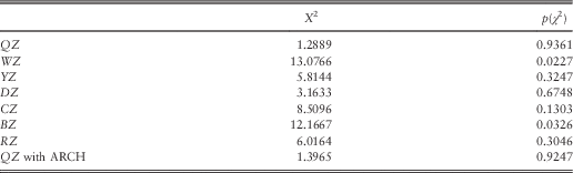
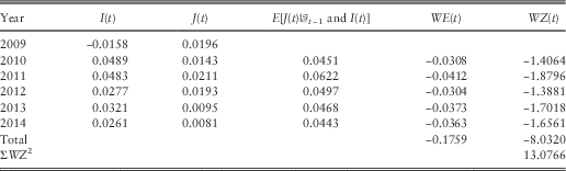
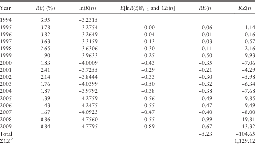
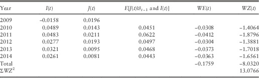
2.12. In Table 1, we see that the values of X 2 for WZ and BZ are larger than for the other series. In Table 2, we show the details for WZ, assuming Model W1 (with WA=0 – see Part 1, ¶3.5). For each year the values of WE(t) and hence WZ(t) are negative, and the values of WZ(t) are in each case between −2 and −1. Thus, the wage index has increased by less than would have been expected given the rates of inflation experienced the structure and parameters of the model. Ft−1 means all the data given at time t−1.
Comparison of actual and expected values of J(t), 2009–2014 conditional on Ft−1 and I(t), using Model W1.
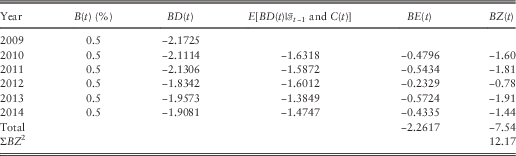
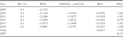
2.13. In Table 3, we show the corresponding figures for B. Bank Base Rate in the United Kingdom, which we use as an indicator of short-term interest rates, was reduced to 0.5% in March 2009, and it has remained there since then. We commented in Part 1 on the exceptionally low value of B(t) and hence BD(t) in June 2009. The values of long-term yields, indicated by C(t), have varied, and so therefore has BD(t). However, the model “expects” BD(t) and hence also B(t) to revert to more like their “normal” values, and in each year they have not done so. Hence the value of X 2 is large, at 12.1667, with a probability of 0.0326; this is not too extreme, but is nevertheless worth comment.
Comparison of actual and expected values of BD(t), 2009–2014, conditional on Ft−1 and C(t).
2.14. In Part 1, we made the suggestion that practitioners might like to take the value of QMU as 0.025 for the future, being more in line with the policies of the UK government and the Bank of England. In fact the one-step-ahead results show a rather lower value of X 2 at 1.2184, with a correspondingly higher value of p(χ 2) of 0.9048; but these values are also quite unremarkable.
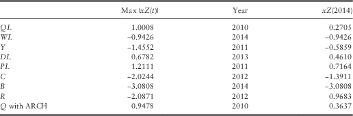
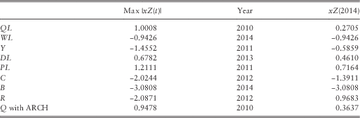
2.15. In Table 4, we show results of the 5-year forecast, in which the values of different variables in 2014 are compared with those expected in 2009. All are unexceptional, except for B(t), which again is shown to be significantly lower than might have been expected in 2009, even allowing for the fact that its value was 0.5% even then. However, although it has been unusual in recent years for Bank Base Rate to remain unchanged for so long as it has now, we should note that its predecessor, then called Bank Rate, remained at 2% from June 1932 to November 1951, except for 2 months in mid-1939, so long periods of stability are not unknown.
Values of xZ(2014), that is, the error in forecasting the Z residual, and the maximum value of |xZ(t)| and the year in which it occurred, for multi-year forecasts from 2009.
2.16. With extra data it is possible to calculate the new maximum likelihood estimates of the parameter values. We have done this, but the results are so little different from those given in Part 1 that we think it would be confusing rather than helpful to quote them, though the model for B may require reconsideration in due course.
3. Different Sets of Variables
3.1. Any model like the Wilkie model is designed for use by random simulation, nowadays often under the name of an “economic scenario generator”. Often one starts at some simulation time t=0, generates a set of random numbers from some distribution from which random innovations can be calculated and calculates the values of suitable variables for the next time step, t=1. This is continued step by step to some final time t=T. We can carry out S similar simulations, all starting at t=0 and continuing to t=T, in parallel. We would have S different end-points and a total of S×T simulated “nodes”, excluding the first starting node at t=0. If we chose T=10 and S=100,000, we would have one million nodes.
3.2. An alternative method that may be useful in some applications is to use a branching or tree structure. One simulates from t=0 to t=1 say ten times. From each of the end-points at t=1 one simulates say ten times to t=2, giving now 100 nodes. From each of these one can simulate again ten times to t=3, following this up with a narrower tree, where only two new branches are simulated at each time step. If this continues to t=10, we would have 103×27=128,000 end-points, and have 255,100 simulated nodes.
3.3. If we use a binary tree with two branches at each node we would have only 1,028 end-points over 10 years, and 2,046 simulated nodes. This seems to us rather sparse, though there are some situations where a binary pattern may have its advantages. Using three branches at each node gives us 59,049 end-points and 88,572 nodes. Using four gives us 1,048,576 end-points and 1,398,100 nodes. As the required time for a simulation is probably proportional to the number of nodes simulated, this is not much more costly than 100,000 parallel simulations, and the much larger number of end-points may have its advantages.
3.4. In order to simulate in a tree structure it is necessary to hold enough data to go back to earlier nodes in the tree. A convenient method of simulating a tree structure might be to do one linear simulation from t=0 to t=T, counting this at taking the first (or “left-hand”) branch at each node. We might denote this as “1, 1, … , 1, 1” with T sequential numbers. We then back up one node to t=T−1 and simulate a second branch from T−1 to T giving the sequence “1, 1, … , 1, 2”. If we are following our tree as defined in ¶3.2 we would then back up two steps to t=T−2, and add sequences ending in “… , 2, 1” and “… , 2, 2”. We carry on moving backwards and forwards until we end up with the sequence “10, 10, 10, 2, … , 2, 2”. At any time we need the data for all previous nodes, so that we can back-track to that node and start again from there. We call the set of data required for each node the “working set”; it may also be called the “state space” but this has a wider connotation. In a purely linear simulation the same data is necessary, but it is not so essential to identify it and to store it.
3.5. There may be a choice of exactly what variables are in the working set. They are most conveniently chosen to make the calculations easier, but the variables are not necessarily the same as those that are convenient to pass in as inputs at time t=0 to establish the starting point, nor are they necessarily those that are most convenient to provide as output.
3.6. We exemplify this by discussing the model for inflation:
 $$\eqalignno{ QE(t)& =QSD.QZ(t) \cr IN(t)& =QA.IN(t{\minus}1){\plus}QE(t) \cr I(t)& =QMU{\plus}IN(t) \cr QL(t)& =QL(t{\minus}1){\plus}I(t) \cr Q(t) &={\rm exp(}QL(t){\rm )} $$
We can see that if we hold the values of IN(t) and QL(t) for time t we can readily progress to time t+1. We simulate a new value for QZ(t+1), hence calculate QE(t+1), IN(t+1) and I(t+1). We can then put:
 $$QL(t{\plus}{\rm 1})=QL(t){\plus}I(t{\plus}1)$$
from which we can, if we wish, get Q(t+1), but we use QL(t) in the working set. We could alternatively use in the working set I(t) instead of IN(t) and Q(t) instead of QL(t), but this would require more calculations in each step, and with very large numbers of steps to calculate, any small efficiency is valuable.
3.7. Although it is convenient to use IN(t) and QL(t) in the working set, these are not convenient for the initial input, for which I(0) and Q(0) are better. Q(−1) could be used instead of I(0) because I(0) can easily be calculated as lnQ(0)−lnQ(−1), but we prefer in general to use I(0). The value of Q(0) can be chosen arbitrarily. Q(t), like W(t), P(t) and D(t), is a ratio scale, in that all that are interesting are the various ratios Q(t 1)/Q(t 0) or equivalently lnQ(t 1)−lnQ(t 0), and values derived from these. One could choose Q(0)=1 or 100, or the value of the current price index, as desired.
3.8. It is worthwhile being economical with the output. What is eventually needed will depend very much on the application that is being considered, but if one wishes to store the output for each step of each simulation, then the quantity can be very large. In this case, values of Q(t), for all steps (including t=0) give the minimum that is needed, because values of I(t) for each step can be calculated from these. However, the ultimate application may not wish to retain either of these variables, but just to use them for some other purpose and then discard them; or it may need other variables from the model, and not need a price index or a rate of inflation at all.
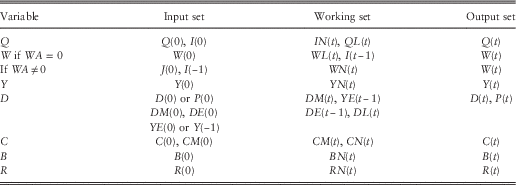
3.9. It would be tedious to go through every variable in the same way, so we just show in Table 5 our suggested sets of input variables, working variables and output variables for each part of the model. In each line only variables that are additional to those already stated are noted.
Suggested input sets, working sets and output sets of variables.
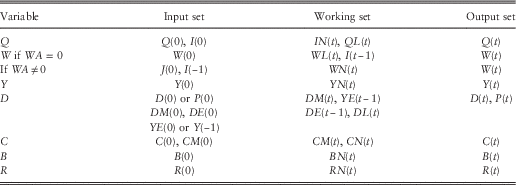
3.10. Some comments are necessary. For the wages model we need both I(t), which we get from IN(t), and also I(t−1), which therefore needs to be held as part of the time t working set, so we denote it also as IP(t) (P for “previous” and we put YEP(t)=YE(t−1), etc.). If WA is included at a non-zero value, so that there is some autoregression in the “real” wages increments, then we need to calculate WN(0) for which we need both J(0) and I(−1), that is, inflation in the year one previous to the last year at time 0. For the dividend model we need a starting value for D(0); we can either insert this directly, in which case the value of P(0), the share price index, can be calculated from it and Y(0), or we can input P(0) and calculate D(0) from it. For this model we also need YE(0) to calculate K(1); this can either be given directly or can be calculated if Y(−1) is given. More complicated are the long-run moving-average terms, DM(0) and CM(0). To calculate these we need a long run of past values of inflation. Likewise, the value of DE(0) depends on a long-run calculation based on past values of Q(.), D(.) and Y(.). To help potential users of the model we show certain of these values in section 4; but these are based on the 2009 parameters, and would be altered if another set of parameter values were to be used.
4. Initial Conditions
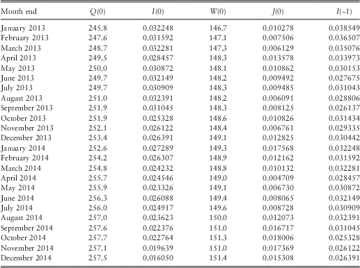
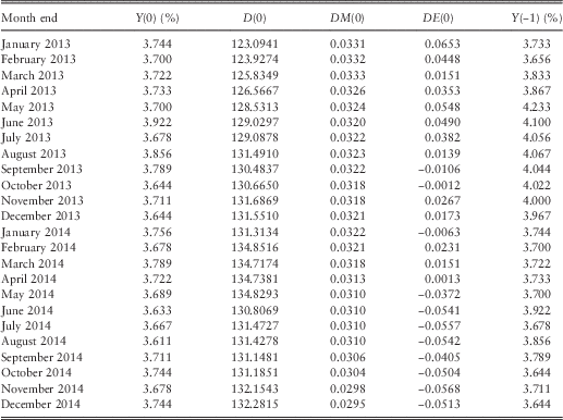
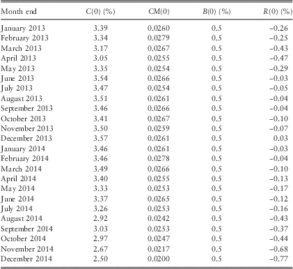
4.1. We have shown in section 3 the set of variables that is needed for initialising any set of simulations, what we have called the “initial conditions”. These can be the market conditions at any chosen date, or any arbitrary set of values, or a set of “neutral initial conditions”, which we discuss in sections 5 and 6. We start by showing in Tables 6–8 the sets of market initial conditions for the United Kingdom for the end of each month during 2013 and 2014.
Initial conditions for the retail prices and wages models in 2013 and 2014.

Initial conditions for the dividend yield and dividend index models in 2013 and 2014.
Initial conditions for the interest rate models in 2013 and 2014.
4.2. The index used for prices is the UK Index of Retail Prices. Advantages of this over the Consumer Price Index (CPI), which is also published, are that the published value is never revised, so that by the middle of the month, after that to which it applies, the value is known. For wages we now use the UK index of average weekly wage rates. This may be less appropriate for actuarial uses, such as the liabilities of salary-based pension funds or the expenses of insurance companies, than the formerly published index of average monthly earnings. The different UK wages indices are frequently revised and rebased, which requires us to alter the chain-linking with earlier indices. Thus, the values given here may not be consistent with the values published in Part 1.
4.3. The index used for shares in Table 7 is the FTSE-Actuaries All-share index published daily in The Financial Times and accessible on the FT web site (through http://markets.ft.com/ RESEARCH/Markets/Data-Archive). This index has been published continuously since April 1962, though the constituent companies have been changed frequently. In order to keep continuity with previous dividend yield indices, we calculate a notional “gross” yield by ratioing the published “actual yield” by 10/9. This allows for a notional tax rate of 10%. To get the published yields, which may be more convenient for current use, multiply the figures shown by 0.9. If actual yields are to be used, it is consistent to multiply the value for YMU suggested in ¶2.6 also by 0.9, giving 0.03375. But this depends on the tax assumptions that one wishes to make in the simulation application. We have calculated the value of the dividend index, D(0), by multiplying the given share price index value by the value of the grossed up dividend yield.
4.4. The values of DM(t) are calculated from a long (theoretically infinite) series of past values of I(t). The formula given in ¶2.6 is:
 $$DM(t)=DD.I(t){\plus}({\rm 1}-DD).DM(t-{\rm 1})$$
This can be expanded:
 $$DM(t)=DD.I(t){\plus}({\rm 1}-DD).DD.I(t{\minus}{\rm 2}){\plus}\,\,\cdots\,\,{\plus}({\rm 1}-DD)^{k{{\minus}{\rm 1}}} .DD.I(t{\minus}k){\plus}\,\,\cdots\,$$
Calculations using the suggested value of DD of 0.16 show that the coefficients decline fairly slowly, going below 0.001 when k=30, below 0.0001 when k=43 and below 0.00001 when k=56. So to get precise values one would need a long run of data. But as this variable is intended to represent the influence of past inflation on share earnings and hence share dividends, and as one would not seriously expect that inflation many years ago still had an active influence, it may be quite satisfactory to use a much shorter period back, setting perhaps the first used value of DM(.) to be the same as the value of I(.) at the same date. The values shown in Table 7, however, use values starting in 1901, simply because they are available.
4.5. The value of DE(0) also depends on a long run of past history, and the values shown in Table 7 are based on our data from 1919. But if one started the calculations 10 years ago, there would be differences only in the last decimal place of the values for DE(.) shown in Table 7.
4.6. For long-term interest rates, C(.), we have used a succession of indicators, starting with the yield on 2.5% Consols, which is available historically, then the yield on the Irredeemables Sector of the FTSE-Actuaries BGS indices, which in recent years has included only 3.5% War Loan. However, the yield on War Loan has often not been in line with the rest of the market; in the past the interest on it was paid gross, without deduction of tax, so it was popular with those who did not need to (or perhaps did not wish to) pay tax, and it had rather a high price and a low yield. The taxation system changed for all government stocks in the mid-1990s, so the premium price disappeared. However, as interest rates have fallen the possibility of War Loan being redeemed has risen; and the British Government has now redeemed it at par on 9 March 2015. This was an option in favour of the government, and against the holders, so the price was relatively low and the yield relatively high. With the issuing of some quite long-term redeemable stocks, the published FTSE-Actuaries indices have included a 45-year redemption yield, and since March 2009 we have used the value of this index. Since April 2014 this has been a “par yield” rather than a redemption yield.
4.7. For short-term interest rates, B(.), we use the Bank Base Rate published by the Bank of England. This rate may remain the same for quite long periods, and has been at 0.5% since March 2009, but it has the advantage of being available for a very long historical period. An alternative in recent years might have been to use one of the many short-term LIBOR rates, but these rose very sharply in 2009 as a result of fears about the credit-worthiness of banks, and recent revelations about the dubious way they have been calculated make them less suitable.
4.8. For R(.), the real rate on index-linked stocks, we use the real yield on the “over 5 years” index of the FTSE-Actuaries BGS indices, calculated assuming 5% inflation. There is now enough data to construct a yield curve for index-linked stocks, rather than using one rate to represent all terms, but we have not yet done this.
4.9. The values of CM(.) are, in the first place, like those of DM(.), calculated recursively from past values of I(.), and, with the suggested value for CD of 0.045, the factors decline even more slowly. However, the values of CM(.) are subject to the Min(.,.) function given in ¶2.7. If the minimum “bites” so that the recursive value is replaced by C(t)−CMIN, then the past history is irrelevant. With CMIN=0.005, this occurred at every month end from September 2011 to November 2012, so no values of CM(.) before those dates are needed for the calculation of future market initial conditions.
4.10. We can observe about the use of market conditions that all the values in the stock market indices are available at the close of business each working day, so there is no delay in the possibility of using them. The Retail Prices Index (RPI) for each month is published usually in the 2nd week of the following month, but a close estimate of it can usually be made immediately if it is required. The average earnings indices are published about 2 months after the applicable date, are often revised in the following month and sometimes are heavily revised for some years back. This is inconvenient.
5. Neutral Initial Conditions
5.1. We now turn to what we call “neutral initial conditions”. Wilkie (Reference Wilkie1986) introduced these without giving any formal definition, but the values he gave show that these can be defined in two ways, either as the values to which certain variables would tend if the model were to be projected forward from any starting point with no future innovations, or, with the same results, as the values which, if used as initial conditions and projected forward with no future innovations, would remain unchanged.
5.2. Both these definitions can be developed algebraically. For a straightforward first-order autoregressive time-series AR(1) model, such as for I(t), we have:
 $$I(t{\plus}k)=QMU{\plus}QA^{k} .(I(t)-QMU){\plus}{\rm terms}\,{\rm involving}\,{\rm future}\,{\rm values}\,{\rm of}\,QE(.)$$
from which we see that if future innovations (the QE(.) terms) are zero, then I(t+k) tends to QMU as k tends to infinity, provided that QA<1, as in practice it is. Alternatively, we can seek the values of I(t+1) and I(t) such that I(t+1) is derived from I(t) using the formula but with zero innovation, and such that I(t+1)=I(t). This is seen to be when:
 $$I(t{\plus}{\rm 1})=QMU{\plus}QA.(I(t)-QMU)=I(t)$$
or when I(t+1)=I(t)=QMU.
5.3. If I(t) is stationary and constant, then Q(t) is not stationary, but increases without limit, unless QMU=0. However, it will tend to increase in proportion to Q(0).exp(t.QMU), or, on a graph with a vertical log scale, on a line parallel with this. As already noted, the initial values of Q(0), W(0) and D(0) can be chosen arbitrarily.
5.4. Using these methods we can quickly derive neutral initial conditions of this type, with the following formulae and values, calculated using the parameter values suggested in section 2:
 $$\eqalignno{ I(0)&=I({\minus}{\rm 1})=QMU=0.0{\rm 43} \cr J(0)&=(WW{\rm 1}{\plus}WW{\rm 2}).QMU{\plus}WMU=0.0{\rm 5741}0 \cr Y(0)&=YMU.{\rm exp(}YW.QMU{\rm )}=0.0{\rm 4}00{\rm 8455}={\rm 4}.00{\rm 8455}\,\%\, \cr DM(0)&=QMU=0.0{\rm 43} \cr K(0)& =QMU{\plus}DMU=0.0{\rm 54}0 \cr CM(0)&=QMU=0.0{\rm 43} \cr C(0)&=QMU{\plus}CMUL=0.0{\rm 653}={\rm 6}.{\rm 53}\,\%\, \cr B(0)& =C(0).{\rm exp(}\!\!-\!\!BMU{\rm )}=0.0{\rm 55}0{\rm 9131}={\rm 5}.{\rm 5}0{\rm 9131}\,\%\, \cr R(0)& =RMU=0.0{\rm 3}={\rm 3}\,\%\, $$
Further, we assume that YE(0)=0 and DE(0)=0. Future values of these innovations are also assumed to be zero for this purpose.
6. Long-Term Means and Variances
6.1. Alternative definitions of “neutral initial conditions” can be chosen. We could choose the long-run, or unconditional, means of the values. In some ways the long-term means may be more justifiable than those given in section 5, because they represent the mean values that the state variables might take if one looked in on the process at an unspecified time, unconditional on any specific past history.
6.2. In this section and in Appendix we discuss the long-term means, and also the long-term variances and covariances, calculated using the methods described in appendix E of Wilkie (Reference Wilkie1995), but developed further. The long-term means in some cases depend on the distribution of the innovations. If the model is wholly linear, then the defined mean and variance are the same for all distributions of innovations (so long as they have finite variance), though, if the distribution is not symmetrical about the mean, the long-term mean need not be the same as the median or as the neutral value shown in section 5. However, if the model includes non-linear parts, such as exponentiation, the situation is different. If we assume that the innovations, the XE(.) values, are normally distributed, or equivalently that all the XZ(.) values are unit normal, then, as the exponential of such a normally distrusted variable is distributed lognormally, the long-run mean is not the same as what we have shown in section 5 for a neutral value.
6.3. Another possibility is to use a randomly selected set of initial conditions, drawn from their unconditional or long-term distribution. For this one needs the means, variances and covariances which we have shown. But it is then convenient, and equally valid, to use only linear elements of the model, so that the selected set of variables could be the same as the working set, omitting those, like QL(t) and WL(t), that are scale variables:
 $$IN(t),\,IP(t),\,WN(t),\,YN(t),\,YEP(t),\,DM(t),\,DEP(t),\,CM(t),\,CN(t),\,BN(t),\,RN(t)$$
The mean of I(t) is equal to the mean of IN(t) with the addition of QMU, and the variance and covariances are the same as those of IN(t). The same is true for CN(t) and CRL(t), BN(t) and BD(t), and RN(t) and R(t). But the similar relationships do not apply for J(t) and YL(t), where other elements come in, so it is interesting to show the means, variances and covariances for these and for K(t), and over a finite period, for QL(t), WL(t), DL(t) and PL(t). The means and variances of these normally increase without limit as time tends to infinity; we say “normally”, because with particular parameter values the means may remain constant, such as if QMU=0.
6.4. Another way of estimating the same result would be to start with any set of initial conditions, run the simulations for a quite long period and to start each effective simulation at the point that one had now reached, in effect using a long run-in period. The length of the desirable run-in period is worth investigating.
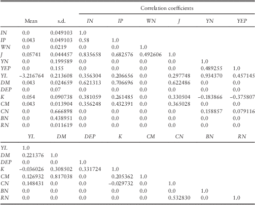
6.5. In Appendix we show the formulae for the means and variances for many relevant variables, including all those that we might need as initial conditions, at time 0+t, given the data at time 0, and also the formulae as t→∞, that is, the long-term means and variances. In addition, we show the formulae for the covariances between pairs of variables, from which the correlation coefficients can be calculated. In Table 9 we show the numerical values of these long-term statistics, assuming the parameters suggested in Part 1 and in section 2 of this paper.
Means, standard deviations and correlation coefficients of variables given.
6.6. Those who wish to start a simulation at a random point can use the values in Table 9 to pick random starting values of the state variables, probably after converting the correlation matrix to its Cholesky decomposition. If different parameter values are to be used, then the formulae in the Appendix can be used to construct modified tables.
6.7. We can also note that:
 $$\eqalignno{ E{\rm [}I(\infty){\rm ]}& =E{\rm [}IN(\infty){\rm ]}{\plus}QMU=0.0{\rm 43} \cr E{\rm [}CRL(\infty){\rm ]}& =E{\rm [}CN(\infty){\rm ]}{\plus}CMUL=-{\rm 3}.{\rm 8}0{\rm 32} \cr E{\rm [}BD(\infty){\rm ]}& =E{\rm [}BN(\infty){\rm ]}{\plus}BMU=0.{\rm 17} \cr E{\rm [}R(\infty){\rm ]}& =E{\rm [}RN(\infty){\rm ]}{\plus}RMU=0.0{\rm 3} $$
and that the standard deviations and correlation coefficients are the same as those of the corresponding zero mean variable.
6.8. Using the fact that, if X is lognormally distributed so that ln(X) is normally distributed with mean µ and variance σ 2, then E[X]=exp(µ+σ 2/2) and Var[X]=E[X]2.(exp(σ 2)−1), we get:
 $$\eqalignno{ E{\rm [}Y(\infty){\rm ]}& ={\rm exp(}\!\!-\!\!{\rm 3}.{\rm 2168}{\plus}0.0{\rm 456}/{\rm 2)}=0.0{\rm 41}0 \cr {\rm Var[}Y(\infty){\rm ]}& =0.0{\rm 41}0^{{\rm 2}} .({\rm exp(}0.0{\rm 456)}-{\rm 1})=0.0000{\rm 7851} \cr {\rm s}{\rm .d}{\rm .[}Y(\infty){\rm ]}& =\ ^\surd\!\!{\rm Var[}Y(\infty){\rm ]}=0.00{\rm 89} $$
and
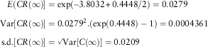 $$\eqalignno{ E{\rm (}CR(\infty){\rm ]}& ={\rm exp(}\!\!-\!\!{\rm 3}.{\rm 8}0{\rm 32}{\plus}0.{\rm 4448}/{\rm 2)}=0.0{\rm 279} \cr {\rm Var[}CR(\infty){\rm ]}& =0.0{\rm 279}^{{\rm 2}} .({\rm exp(}0.{\rm 4448)}-{\rm 1})=0.000{\rm 4361} \cr {\rm s}{\rm .d}{\rm .[}CR(\infty){\rm ]} &=\ ^\surd\!\!{\rm Var[}C(\infty){\rm ]}=0.0{\rm 2}0{\rm 9} $$
6.9. Observing that CM and CR are independent, we then get:
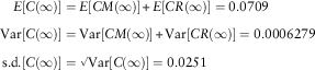 $$\eqalignno{ E{\rm [}C(\infty){\rm ]} &=E{\rm [}CM(\infty){\rm ]}{\plus}E{\rm [}CR(\infty){\rm ]}=0.0{\rm 7}0{\rm 9} \cr {\rm Var[}C(\infty){\rm ]}& ={\rm Var[}CM(\infty){\rm ]}{\plus}{\rm Var[}CR(\infty){\rm ]}=0.000{\rm 6279} \cr {\rm s}{\rm .d}{\rm .[}C(\infty){\rm ]}& =\ ^\surd\!\!{\rm Var[}C(\infty){\rm ]}=0.0{\rm 251} $$
Now, if we assume first that CR(∞) is approximately normally distributed, so that C(∞) is approximately normally distributed, and then, in contradiction of that, that C(∞) is approximately lognormally distributed, so that CL(t) is approximately normally distributed we get:
 $$\eqalignno{ {\rm Var[}CL(\infty){\rm ]}&={\rm ln(}0.000{\rm 62786}/0.0{\rm 7}0{\rm 9}^{{\rm 2}} {\plus}{\rm 1)}=0.{\rm 1178} \cr E{\rm [}CL(\infty){\rm ]}& ={\rm ln(}0.0{\rm 7}0{\rm 9)}-0.{\rm 1178}/{\rm 2}=-{\rm 2}.{\rm 7}0{\rm 61} \cr {\rm s}{\rm .d}{\rm .(}CL(\infty){\rm )}& =0.{\rm 3433} $$
6.10. This allows us to derive statistics for BL(∞)=CL(∞)−BD(∞):
 $$\eqalignno{ E{\rm (}BL(\infty){\rm ]}& =-{\rm 2}.{\rm 7}0{\rm 61}-0.{\rm 17}=-{\rm 2}.{\rm 8761} \cr {\rm Var[}BL(\infty){\rm ]}& =0.{\rm 1178}{\plus}0.{\rm 1927}=0.{\rm 31}0{\rm 5} \cr {\rm s}{\rm .d}{\rm .[}BL(\infty){\rm ]}& =0.{\rm 5572} $$
and then if we assume, again in contradiction, that BL(∞) is lognormally distributed, we can get:
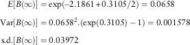 $$\eqalignno{ E{\rm [}B(\infty){\rm ]}& ={\rm exp(}\!\!-\!\!{\rm 2}.{\rm 1861}{\plus}0.{\rm 31}0{\rm 5}/{\rm 2)}=0.0{\rm 658} \cr {\rm Var[}B(\infty){\rm ]}& =0.0{\rm 658}^{{\rm 2}} .({\rm exp}(0.{\rm 31}0{\rm 5})-{\rm 1})=0.00{\rm 1578} \cr {\rm s}{\rm .d}{\rm .[}B(\infty){\rm ]}& =0.0{\rm 3972} $$
6.11. When a lognormal distribution has a small standard deviation it is almost indistinguishable from a normal one. With σ=0.05, the distribution and density functions are almost the same; with σ=0.1 they are still quite close; with σ=0.2 they are noticeably different. The standard deviations of YL and of CRL are bigger than 0.2, so our approximations are not very good. Further, we have made no allowance above for the Max(.) function in the calculation of CM. An alternative approach is to estimate some of these answers by simulation, as we discuss below.
6.12. The various means, variances and covariances that do converge to a finite limit, do so at different speeds, and for the means the convergence depends on the initial values. The means that converge most slowly are those for CM, CRL and R, where the relevant factors CDC=1−CD=0.955, CA=0.92 and RA=0.95 are large, meaning that the past retains a stronger influence. The mean for CM is the slowest but even so it is within about 1% of its final value by about 70 years, and within 0.1% by 120 years. But these periods do depend on the initial conditions, for which we have used those in June 2014.
6.13. The convergence of the standard deviations and correlation coefficients does not depend on the initial conditions, and is rather faster. The same variables have the slowest convergence. The standard deviation for CM and also the correlation coefficients involving CM are within 1% of their final values by 45 years and within 0.1% by 70 years. So a run-in period of 100 years would seem to be ample.
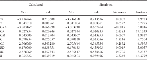
6.14. We have carried out one million simulations of the model, each for 500 years, using the parameters noted above and the initial conditions as at June 2014. These allow us to confirm our formula calculations, and to make estimates of other values.
6.15. In Table 10, we show the means and standard deviations of the variables discussed above, first, as calculated above from the theoretical values at infinity, and second, as simulated at year 500 in our 1,000,000 simulations. We can see first that for the variables that are normally distributed, YL, CRL, CM and BD, the simulated means and standard deviations are very close to the theoretical ones, and the skewness and kurtosis coefficients are close to zero and 3.0, as is appropriate for a normally distributed variable. The means and standard deviations of the other variables are quite close to what we calculated above. We can take it that Y and CR are indeed lognormally distributed, but we can see that CL is not normally distributed, with negative skewness (−0.29) and quite high kurtosis (4.6), and that BL is also not normally distributed, with slight negative skewness (−0.07) and rather high kurtosis (3.24).
Statistics of selected variables as calculated and as simulated.
6.16. In the simulations we have also recorded the values of CM unadjusted for the Max(.) criterion and CM adjusted for it. The results depend on the initial conditions as well as on the values of QMU (0.043) and CMIN (0.5%), but we can observe that with these parameters both CM unadjusted and CM adjusted converge close to their ultimate values of 0.043 within 100 years, and the long-term difference between then stabilises at about 0.0000025, a very small value. The maximum function “bites” in about 1.5% of simulations, on average for about 2.2 years in each simulation in which it occurs, in effect in 1 year in about 15,000.
6.17. We have also done the same calculations with a lower value of QMU of 0.025. This increases the proportion of simulations in which the maximum bites to about 36%, with an average of 3.5 years out of 500 in each simulation, in effect in 1 year in about 390. The difference between the two values of CM is about 0.00013, compared with the mean of 0.025. Thus, although the limitation occurs much more often, the effect is not large.
6.18. In a third trial we retained QMU=0.043, but reduced the value of CMIN to 0.0001%. This reduces the effect of the constraint, so that it occurs in about 0.4% of simulations, for an average of 2 years in each simulation, or 1 year in about 60,000 years. The difference between the two values of CM is about 0.00000075, a trivial amount. As our choice of CMIN as 0.5% was arbitrary, and all that is needed is a value above zero, so that we can take the logarithm of CR, a tiny value seems satisfactory, especially since short-term rates (though not long-term ones) are now extremely low and in some countries even negative.
6.19. Although we describe the constraint as biting in one in so many years, the occasions are not evenly distributed, but tend to occur in groups. One needs I(t) to be negative, and CR(t) to be small, and as these are both autoregressive processes, the necessary conditions may apply for several years in succession.
7. Neutralising Parameters
7.1. A model like the Wilkie model, which indicates different expected returns in stock markets at different times, can be criticised by those who adopt an “efficient market” approach, roughly on the lines: “If you are expecting the prices of shares to fall (e.g. because of a very low dividend yield) and others agreed with you, would they not have fallen already? So why do you think you, or your model, can outsmart the market?”. We do not discuss the theoretical aspects of this arguments here, but we follow the suggestion of Lee & Wilkie (Reference Lee and Wilkie2000) that one way of reconciling both points of view is to use what we call “neutralising parameters”, that is, to choose values of the parameters, in particular the means of the series, so that the market conditions at any date are the neutral initial conditions for those parameters. One can justify this by assuming that participants in the market do use, for example, the Wilkie model but that the values of the parameters of the model at any time are chosen to reflect correctly “the market’s” view of the future. In what follows we discuss in detail how this might work. It fits some parts of the model more easily than others. We use conditions as at the end of June 2014 as an example, but refer back to other dates where appropriate.
7.2. We assume that we have data up to time t, and that we wish to choose initial conditions and altered parameters at that time in order to start future simulations from time t. We denote values of variables at time t to be used as initial conditions and also parameters altered for the neutralising process by one or more following asterisks *, **, etc., and, as the neutralising parameters depend on time t, we denote that also by a following (t). We can distinguish between those initial conditions which are externally given, which as far as possible we apply as they are, and those which are derived from the past history of the model itself, which include DM(t), DE(t), YE(t) and CM(t). It is not inconsistent with current market conditions to alter these as required, in particular to set DE*(t)=YE*(t)=0 as inputs at time t. Throughout this section we use the definition of neutral initial conditions given in section 5, the central or median values, rather than the long-term means described in section 6.
7.3. The value of I(t) in June 2014 was, as shown in Table 6, 0.0261, and we would wish to set I*(t)=I(t)=0.0261. The neutral initial condition for I(.) is QMU (see ¶5.2). So, if we were to set QMU*(t)=I*(t)=0.0261, then at that date the neutral value of I(.) would be the actual value. In Part 1 we showed that, on the basis of the 1923–2009 data, the maximum likelihood estimate of QMU was 0.0429 with a standard error of 0.0101. So a value of 0.0261 is more than 1 s.e. away, but <2. Thus, 0.0261 is a not unreasonable estimate of the value of QMU for the future, well within a 95% confidence interval.
7.4. However, in June 2009, the observed value of I(t) was −0.0158, and this compares with the previous year’s value of 0.0448 and the subsequent year’s value of 0.0489. There were specific local reasons for the decrease in the UK RPI value over the period 2008–2009, because housing costs in it are represented, not by rents, but by interest payments on loans for house purchase; the sharp drop in general interest rates meant corresponding drops in the payments on house purchase loans, so the value of the RPI fell. However, the value of other inflation indicators, such as the CPI, did not fall. To have taken QMU*(t)=−0.0158, implying a general fall in prices for the foreseeable future, would have seemed perverse at that time, though there are economic circumstances when a long-term fall in prices might seem plausible.
7.5. The RPI value is not, however, determined by market trading, so it cannot easily be argued that “the market” has it right. Different participants in the investment market do have their views on the likely level, or average level, of future inflation. One measure of this might be the “implied inflation”, observed in the fixed interest markets, which we shall take (a little crudely, because we are blurring the difference between annual rates and logarithmic estimates and ignoring yield curves for different terms) as the difference between C(t) and R(t), our measures of long-term conventional fixed interest rates and the rates on index-linked stocks. For “implied inflation” we can put II(t)=C(t)−R(t). At the end of June 2014 this was 3.49%, rather higher than the value of I(t) at that date; the value in June 2009 was very similar at 3.55%. An alternative view of a market estimate of QMU*(t), which we shall denote QMU**(t) at that time might therefore be 0.0349.
7.6. We have data at monthly intervals for a long period, with values of R(t) since May 1981, so we can calculate what the values of QMU*(t) and QMU**(t) would have been since that date. The latter is rather more stable than the former. QMU*(t) varies from −0.0158 (in June 2009) to 0.1137 (in December 1981), whereas QMU**(t) varies from 0.0242 (in September 1998) to 0.1096 (in September 1981). We plot them in Figure 1, and one can see that QMU** is much more stable than QMU*, and therefore it might be a better candidate as a neutralising parameter. However, using its value at any time means that the expected central path of I(t) from whatever its value is to its long-term central value, is curved, so if I(t)≠QMU**(t) we are making an implicit forecast of future values of inflation in the short term.
Values of QMU* and QMU**, 1981–2014.
7.7. When we move on to wages, W(t), we have similar problems. Wages are not set by the stock market, and there is no obvious market in which expectations of future wage growth are traded. The value to be selected is WMU, and the neutralised value of that is:
 $$WMU^{\asterisk}\!(t)=J(t){\minus}(WW{\rm 1}{\plus}WW{\rm 2}).QMU^{\asterisk}\!(t)$$
We could, alternatively, use QMU** giving an alternative value:
 $$WMU^{\asterisk \asterisk\!}(t)=J(t){\minus}(WW{\rm 1}{\plus}WW{\rm 2}).QMU^{\asterisk \asterisk}\!(t)$$
7.8. In June 2014, J(t)=0.0087, so WMU*(t)=−0.0140 and WMU**(t)=−0.0216. Both have been negative since 2009, and both have been negative at intervals before that. This can be seen from Figure 2; note that it is not on the same vertical scale as Figure 1. One can also see that both WMU* and WMU** are variable. This is all rather uncomfortable. As our parameter values show WW1+WW2=0.87, wages are not credited with the full rate of growth of prices, and WMU needs to be at least a small positive number for wages in the long run even to keep pace with prices. In the data that we have, which goes back to 1809, there has been a small, but steady, positive real growth of wages, of about 1.3%, and this rate of growth has been fairly steady over quite long periods. So a change to a negative rate of growth of real wages would indicate a very different sort of economy than we have had for a long time. As there are no market conditions influencing our choice of a value for WMU, perhaps leaving it at the fitted value of 0.020 is as good as any.
Values of WMU* and WMU**, 1981–2014.
7.9. We now consider, Y(t), the dividend yield. This is straightforward. We can put either:
 $$YMU^{\asterisk}\!(t)=Y(t).{\rm exp(}{\minus}YW.QMU^{\asterisk}{\rm )}$$
or
 $$YMU^{\asterisk \asterisk}\!(t)=Y(t).{\rm exp(}{\minus}YW.QMU^{\asterisk \asterisk}{\rm )}$$
depending on which version of the neutralised mean rate of inflation we wish to use. In either case the value of YMU*(t) or YMU**(t) is a little less than the value of Y(t), and their values are very close (see Figure 3).
Values of YMU* and YMU**, 1981–2014.
7.10. The share dividend yield is the most fundamental element in the neutralisation. It is one item that is wholly controlled moment to moment by the market, whereas share dividends, the other factor in share prices, depend on decisions by the directors of companies from time to time. The next step in the sequence of the model would be to consider share dividends, D(t), but we leave these till after we have considered interest rates.
7.12. We start our consideration of interest rates with the real yield on index-linked stocks, R(t). We have not yet modelled a yield curve for index-linked stocks, though this is obviously desirable and is now possible, which it was not when the Wilkie model was first published. We hope to consider this in a later part of this series. The neutralising value for R(t) is simple. We put RMU*(t)=RMU(t); there are no other influences. In June 2014, the value, at −0.12%, was negative as it has been for most of the time since late 2011. One may think that to accept a negative yield, even on an inflation protected stock, is unwise or even irrational, but there are local reasons in the United Kingdom which justified this; the UK government is the only issuer; the supply is quite large, but still limited; UK pension funds and insurance companies wish to invest heavily in such bonds to match the index-linked pensions they have promised to pay; so for these reasons a small premium in the price may exist. Moreover, to make the current market value neutral, we have no other choice.
7.13. The more difficult variable is the long-term interest rate, C(t). We need to consider both this and CM(t), because both are needed as initial state variables. The obvious way to do this is to alter CM(t) to equal QMU* or QMU**, and to calculate CMU*(t) by C(t)−QMU*(t), but this fails because we need to take the logarithm of CMU* and this is not possible if it is zero or negative. In June 2014, the value of C(t) was 3.37% or 0.0337. Our alternative mean rates for inflation were 0.0261 and 0.0349. The latter would make CMU**(t) negative (and by construction it equals the value of R(t), so it would always have the same sign), though the former gives a value of CR(t) of 0.0076, low but acceptable. Perhaps this exposes a problem with the model. CM(t) was designed to be an estimate of the market’s estimate of future inflation, and was proposed before index-linked stocks had sufficient history to contribute. But a measure such as implied inflation, as we have proposed in ¶7.4, might now be better. The relationship between implied and actual inflation is worth further study, and we hope to consider this also in a later part of this series. We moved, in Part 1, from modelling R(t) rather than ln(R(t)), as in Wilkie (Reference Wilkie1995), because observed values of R(t) had become negative. We might assume, however, that interest rates on conventional bonds would not become negative, though recent events in some other countries (Denmark, Switzerland, Finland) might contradict this.
7.14. A compromise is to take CM*(t) as Min(QMU* or QMU**(t), C(t)−CMIN), and then take CMU*(t) as C(t)−CM*(t). If the constraint applies, this makes CMU*(t) equal to CMIN, a number which has been chosen arbitrarily. This situation would have applied for most month ends in the 3 years from 2010 to 2013. It is not altogether a satisfactory solution, but it does avoid the criticism that the model is trying to outsmart the market.
7.15. The short-term interest rate, B(t), is now straightforward to calculate, but difficult to assess. We put:
 $$BMU^{\asterisk\!}(t)={\rm ln(}C(t)/B(t){\rm )}=BD(t)$$
At the end of June 2014 this had the value of 1.9081; the value of C(t) was 6.7 times that of B(t), or B(t) was about 15% of the value of C(t). This is a quite extreme value. Between January 1900 and December 2008, BMU*(t) ranged from 0.7683 (in October 1977, when B(t)=5%, C(t)=10.78%) to 0.8540 (in December 1907, when B(t)=7%, C(t)=2.98%), corresponding to the value of B(t) ranging from 46% to 2.35 times the value of C(t). Since May 2009 the value of B(t) has been between 10% and 17% of the value of C(t). To use the calculated value of BMU*(t) makes a rather strong assumption about the continuation of the present regime. It seems likely to continue in the short term, but who knows for how long?
7.16. We now revert to the share dividend index, D(t), and the associated value of DM(t). If we choose to use the value QMU*(t)=I(t) defined in ¶7.3, set the value of DM(t) equal to this, set YE(t)=DE(t)=0, to leave no adjustments from the past, then the value of DMU*(t)=K(t)−QMU*(t). In June 2014 this has the value −0.0124. This is a lot lower than the standard value of DMU based on the whole period, of 0.011. But K(t) is very variable, and the value of DMU*(t) so calculated would have ranged from −0.3541 (in May 1932) to 0.2255 (in November 1925); these are many years ago, but the range in very recent years has been almost as great from −0.2619 (in October 2009) to 0.1740 (in June 2008). Even in January 2013 it was 0.0848, so it has fallen a lot in 18 months. We feel that it would be difficult to argue that the market’s view about long-term future real increases in share dividends would change by this much.
7.17. An alternative approach is possible. If long-term bonds yielding C(t) are bought, and any interest income is reinvested also at rate C(t), then the long-term return on such an investment (in money terms) is C(t). The long-term central value of this, as shown in ¶5.4 is QMU+CMU=6.53% with our usual parameters. If long-term index-linked bonds are bought at yield R(t) and interest similarly reinvested, the real yield is R(t). The long-term central value for this is RMU and allowing for inflation at its central value, the long-term money return is RMU+QMU=7.3% with our usual parameters. This is higher than the long-term yield on fixed money bonds because our value of RMU=3.00% is higher than our value of CMU=2.23%. If shares are bought at a dividend yield of Y(t), and dividends are reinvested at the same yield, then the long-term return depends on the rate of inflation and the rate of real dividend growth, added to the initial yield. The central long-term central value of all these elements is YMU.exp(YW.QMU)+QMU+DMU=9.41%. So in the long run, shares carry a premium of 2.88% over long-term bonds, and of 2.11% over index-linked bonds; we denote these premiums as PSC and PSR, respectively, and we assume that they apply at all times.
7.18. We can then apply this rationale to conditions at time t. If long-term bonds yield C(t), we need to adjust the parameters for shares to have a long-term return of C(t)+PSC. We have then to choose what we denote DMU**(t) so that:
 $$Y(t){\plus}QMU^{\asterisk}\!(t){\plus}DMU^{\asterisk \asterisk}\!(t)=C(t){\plus}PSC$$
or
 $$DMU^{\asterisk \asterisk}\!(t)=C(t){\plus}PSC-Y(t)-QMU^{\asterisk\!}(t)$$
As at June 2014 the value of DMU**(t), calculated in this way, was 3.37%+2.88%−3.63%−2.61%=0.01%. This is higher than the value of −0.0124 found in ¶7.15, but it is still rather low. DMU**(t) varies very much less than DMU*(t) but its recent range is from −3.0% (in September 2011) to 6.31% in (May 1993). We would prefer to use a less varying method; but one of our assumptions is that the premium for shares is constant. If instead the premium is assumed to vary with time, we have an extra degree of freedom, and we are left having to use our judgement.
7.19. Another, simpler, method of achieving a sort of market neutrality is to assume that the real rate of return on shares, roughly equal to Y(t)+DMU***(t) (another new variable) remains constant, not adjusting at all to changes in fixed interest rates. Its long-term value is represented by YMU.exp(YW.QMU)+DMU=5.11%. Thus, at time t, DMU***(t) is easily calculated as 0.0511−Y(t). At June 2014 this gives DMU***(t)=0.0148, only a little higher than the constant value of DMU of 0.011. It has been much more stable than our other suggestions, ranging from −0.0668 (in November 1974, when Y(t) equalled 11.79%) to 0.0282 (in August 2000 when Y(t) equalled 2.29%). It is not unreasonable to assume that share prices are bid up to lower than normal yields when the prospects of rises in future dividends are thought to be good, and that they fall to lower prices and higher than normal yields when dividend prospects are thought to be poor. The market was very pessimistic, with good reason, in late 1974, though events turned out differently, and the market was very optimistic, as it turned out with less than good reason, in 1999 and 2000. However, this method does not adjust the expected return on shares to be consistent with fixed interest yields, which some may think unsatisfactory. We show graphs of the three variables, DMU*(t), DMU**(t) and DMU***(t) in Figure 4, from which we see that the last of the three is much more stable than either of the others.
Values of DMU*, DMU** and DMU***, 1923–2014.
7.20. Our conclusions are that using neutralising parameter values has merits, but it is not always easy to make good sense of the values observed in the markets, and one ends up having to use one’s economic judgement about which method, or which values to use.
8. Select Periods
8.1. Any model like the Wilkie model, intended for simulations many years ahead, necessarily contains only endogenous variables, that is, every variable needed has to be simulated by the model. However, for a great deal of econometric forecasting other items that are known at the time, that is exogenous variables, can be used to make shorter-term forecasts of the items of interest. It is possible to use this concept within a real-world model, by the use of a “select period”, as described by Lee & Wilkie (Reference Lee and Wilkie2000).
8.2. We can explain this most easily by some detailed examples. Consider the forecast for inflation, and assume that we use our model with parameters QMU=0.043, QA=0.58 and QSD=0.04. Assume t=0 as at June 2014 and we know that I(0)=0.026088. The model gives the expected value of inflation over the coming year as:
 $$I({\rm 1})=QMU{\plus}QA.(I(0)-QMU)=0.0{\rm 43}{\plus}0.{\rm 58}{\times}(0.0{\rm 26}0{\rm 88}-0.0{\rm 43})=0.0{\rm 33191}$$
with a standard deviation of QSD=0.04.
8.3. However, the Bank of England publishes Inflation Forecasts, see for example its Inflation Report, August 2014 (Bank of England, 2014), based on a much more complicated macro-economic model than ours, with many other variables. It shows more than one forecast based on different assumptions. It is not easy to pick up numerical information from the fan charts, but one can attempt to make rather rough estimates from them. In one forecast for inflation, of a different index, the CPI rather than the RPI, and of the annual rate, not the logged continuous rate, for the next 3 years, our estimates for the mean values of annual rates are about 1.6%, 1.8% and 2.0%, with possible standard deviations of about 1.2%, 1.3% and 1.4%.
8.4. One may wish to use the Bank of England’s forecasts in the model for the relevant periods. But we do not know what distribution the Bank of England assumes. There are two ways of implementing this, one a little more convenient for a 1-year-ahead forecast, the other much more convenient for subsequent years. First, we assume (artificially) that the Bank’s forecasts are distributed lognormally, rather than normally, with the given means and standard deviations, but changing 1.6% into an assumed mean of a lognormal of 1.016. Converting to the parameters of the underlying normal, the “μ” and “σ” equivalents, we get means of about 0.0158, 0.0178 and 0.0197, and standard deviations of 0.0118, 0.0128 and 0.0137, very little different from our first figures.
8.5. We now wish to replace our expected value for inflation from June 2014 to June 2015, that is I(1), originally 0.033191, by the Bank’s equivalent number of 0.0158. The easy way to do this is just to use this value as E[I(1)], ignoring the value generated by the model, but carrying forward this value in the rest of the calculations, and for next year. But as we shall see, this cannot easily be done for the subsequent years. Better is to introduce an offset, QO(t), into the formulae, so that we have, as usual:
 $$I(t{\plus}{\rm 1})=QMU{\plus}QA.(I(t)-QMU){\plus}QE(t)$$
but with QE(t+1)=QO(t+1)+QSD(t+1).QZ(t+1).
The mean of QE(t+1) is QO(t+1) and the standard deviation is QSD(t+1), both of which are used as temporary modifications. By analogy with the actuarial use of a “select period” in mortality tables, we could denote them by the subscript [t]+1, implying a starting point specifically of t.
8.6. To alter our model forecast mean of 0.036706 to the Bank’s means of 0.0158, we need to make QO(1)=−0.021591. We can use the Bank’s standard deviation of 0.0118 as QSD(1) if we wish. To adjust for the next year we need to base our 1-year-ahead forecast on our new forecast for the mean of I(1), which gives a conditional forecast, which we denote E[I(2)|E[I(1)]=0.0158]=0.043+0.58×(0.0158−0.043)=0.027224. To change this to the Bank’s forecast for year 2 of 0.01783 we need to put QO(2)=−0.009424. Note that it would not have been satisfactory to simply put E[I(2)]=0.020873, because that is the expected value in 2016 on the basis of what the Bank knows in 2014. By 2015 conditions will have altered, more data will be available, and possibly the Bank will have changed its forecast for 2016. Similarly, in our simulations, once we have simulated the value for 2015, that is I(1), the model’s forecast for 2016 will depend on this simulated value. So the offset method seems essential.
8.7. Continuing to the next year, the Bank’s mean value is 0.0197, which we assume is conditional on the Bank’s forecast value of 0.00178. Using the same method, we need an offset, QO(3)=−0.008684 to get our conditional forecast to the same point. The Bank offers no forecasts beyond 2017 so we can either use the model with no adjustment, or as successive offsets have reducing values one might use QO(4)=−0.005, and for t≥5 put QO(t)=0.
8.8. The Bank’s estimated standard deviations of 0.0118, 0.0128 and 0.0137 are all much smaller than the model’s value of QSD=0.04, based on a much longer period of varied economic circumstances. In an autoregressive model such as we are using, successive variances, conditional on the data at t=0, would be QSD 2, (1+QA 2).QSD 2 and (1+QA 2+QA 4).QSD 2. The Bank’s values are not far away from what they would be if QA=0.42 and QSD=0.0118. We do not suggest that the Bank does use the same model as we do; we only observe the coincidence. But it would be reasonably consistent with the Bank’s forecasts to use the same values for QSD(2) and QSD(3) as for QSD(1). Instead we would prefer, and perhaps other users also would, to increase the values of QSD in the select period rather steadily towards the “ultimate” value 0.04, for example putting QSD(1)=0.0118, QSD(2)=0.02, QSD(3)=0.03 and for t≥4 putting QSD(t)=0.04.
8.9. For other variables we may not have the same sort of authoritative forecasts as those supplied by the Bank for inflation; but there may still be circumstances that we know about that we wish to take into account. In recent years we have known that certain large banks and other large companies had cut their dividends to zero, and that these companies were large enough to affect the whole index. In earlier years the UK government has introduced dividend controls, and then later has relaxed them, and this exogenous knowledge would have allowed us to modify the model’s forecasts. In general the offset method works nicely for this sort of adjustment.
8.10. A different situation may, however, arise for other series, as in our example about interest rates. Our measure of short-term interest rates, the UK Bank Base Rate has been set at 0.5% since March 2009, though there are indications that it might be increased a little within the next year. So we may wish to establish values for B(1) as say 0.0075 with certainty, and possibly 0.01 for B(2). However, our values of B(.) depend on values of C(.) as well as its on their own random process, BD(t), so applying an offset to BD(t) would not be sufficient. We assume that we still wish to generate values of C(t) randomly. So our preferred method is to say that B(1)=0.0075, with certainty, and then when the value of C(1) has been generated for each simulation, to back out the value of BD(1) that would have generated that value of B(1), and carry it forward. If we wish to fix the value of B(2) at 1% similarly, we can do so, but if we wish to apply uncertainty to it, then it is probably better to work through an offset to BD(2), although this allows the randomly generated value of C(2) to affect the value of B(2).
8.11. Using a select or run-in period has clear advantages in making the model more realistic, but it has to be done with care, and we recommend allowing for the offset method and for the directly fixing method as both being necessary each in appropriate circumstances.
9. Conclusion
9.1. In this paper, we have elaborated on a number of practical aspects of using a stochastic asset model or an economic scenario generator. We have used the Wilkie model as an example, and explained its features very fully, but just the same aspects would apply to any other model. The very simplest model, say a random walk for share total return, would have correspondingly simple features. However, such a simple model is of limited practical use among practising actuaries, so we hope that what we have described for the example we have used is of practical use for those who prefer other comparable models.
Appendix. Statistics of Variables
A.1. General
A.1.1. In this Appendix we give formulae for the means, variances and covariances of many of the variables in the model, including those that are used as the working set. We follow the methods and notation of appendix E of Wilkie (Reference Wilkie1995), and explain new material, in particular covariances, in more detail. We assume that “now” is time 0, and that we know all the relevant facts for t≤0, F0.
A.1.2. The general method is to express each future value of any variable, X(t), as a linear function, consisting of a fixed part, dependent wholly on elements known at time 0, and a future stochastic part dependent on successive innovations, XZ(1), XZ(2), … , up to XZ(t), and possibly other innovations, YZ(0), YZ(1), … , up to YZ(t). As each XE(t)=XSD.XZ(t) and each YE(t)=YSD.YZ(t) the function can be expressed, where there may be zero or more Y terms
 $$X(t)=E{\rm [}X(t){\rm ]}{\plus}\sum_{i\,=\,{\rm 1},t}} \Psi _{{XX}} (i).XSD.XZ(i){\plus}\sum_{i\,=\,{\rm 1},t}} \Psi _{{XY}} (i).YSD.YZ(t)$$
The “Ψ-weights” ΨXX(i) and ΨXY(i) show the dependence of X on XE(i) and X on YE(i), respectively. The variable Y(.) would have a similar formula and if it is dependent on XE(.) as well as on YE(.) then its formula would include weights ΨYX(i) as well as ΨYY(i).
Then  $${\rm Var[}X(t){\rm ]}=\sum_{i\,{=\,{\rm 1},t}} (\Psi _{{XX}} (i)^{{\rm 2}} ).XSD^{{\rm 2}} {\plus}\sum_{i\,{=\,{\rm 1},t}} (\Psi _{{XY}} (i)^{{\rm 2}} ).YSD^{{\rm 2}} $$
and s.d.[X(t)]=√Var[X(t)].
 $${\rm Covar[}X(t),\,Y(t){\rm ]}=\sum_{i\,{=\,{\rm 1},t}} \Psi _{{XX}} (i).{\rm }\Psi _{{YX}} (i).XSD^{{\rm 2}} {\plus}\sum_{i\,{=\,{\rm 1},t}} \Psi _{{XY}} (i)).{\rm }\Psi _{{YY}} (i).YSD^{{\rm 2}} $$
and the correlation coefficient CC[X(t), Y(t)]=Covar[X(t), Y(t)]/{s.d.[X(t)].s.d.[Y(t)]}
A.1.3. Observe that, for a linear model, generally E[X(t)] depends on the values of the state variables at t=0, but not on the values of XSD, etc., whereas Var[X(t)] does not depend on the initial state variables, but does depend on the values of XSD, etc. As t→∞ the dependence on the initial state variables declines to zero. These observations do not apply to an ARCH model, which is more complicated, as the model is non-linear in the innovations.
A.1.4. If it is the logarithm of X(t), XL(t), that is modelled linearly, and if we assume that XL(t) is normally distributed, then X(t)=exp(XL(t)) is lognormally distributed with mean:
 $$E{\rm [}X(t){\rm ]}={\rm exp(}E{\rm [}XL(t){\rm ]}{\plus}{\rm Var[}XL(t){\rm ]}/{\rm 2)}$$
and variance:
 $${\rm Var[}X(t){\rm ]}=E{\rm [}X(t){\rm ]}^{{\rm 2}} .({\rm Var[}XL(t){\rm ]}-{\rm 1})$$
A.1.5. We use a notation for the sum of a geometric series with t terms:
 $${\rm SumGS(}x,\,t{\rm )}={\rm 1}{\plus}x{\plus}x^{{\rm 2}} {\plus}\,\,\cdots\,\,{\plus}x^{t{-{\rm 1}}} =({\rm 1}-x^{t} )/({\rm 1}-x)$$
In Wilkie (Reference Wilkie1995) this was denoted as ä(x, t), but this is specifically an actuarial notation, so we avoid it here. Note that as t→∞ SumGS(x, t)→1/(1−x), provided |x|<1. We assume, throughout, that the values of the parameters are always such that the series is convergent.
A.1.6. Some of the formulae are almost trivially simple. Others require a great deal of tedious algebraic manipulation. In principle, all the linear elements could be expressed as a large VARMA (vector autoregressive moving average) model, in matrix notation, but this would have lost the intuitive understanding that is brought out by many of the explicit formulae.
A.1.8. The formulae for the means can be readily confirmed numerically by recursive calculation year by year, with all innovations zero to give values say X(t), which are the expected values. The formulae for Ψ-weights can be confirmed similarly, by putting XZ(1) as unity, or as some other convenient constant, performing the same recursive calculations with all other innovations zero, to give new values of future variables, say X*(t), then calculating Ψ(t)=(X*(t)−X(t))/XZ(1). The formulae for variances and covariances can be checked by summing the squares or products of the relevant Ψ-weights.
A.2. Expected values
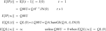
A.2.1. We give formulae for the means, expected values, at future time t, and as t→∞.
A.2.2. Inflation
 $$\hskip-100pt \eqalignno{ E{\rm [}IN(t){\rm ]}& =QA^{t} .IN(0) \cr E{\rm [}IN(\infty){\rm ]}& =0 $$
Note that: E[I(t)]=E[IN(t)]+QMU
 $$\eqalignno{ E{\rm [}IP({t}){\rm ]}& \,=\,{\rm E[}I(t-{\rm 1}){\rm ]}\,=\,I(0)\quad \quad \ \qquad t\,=\,{\rm 1} \cr \quad \quad \quad \quad \quad \;\;\quad \quad \quad &\,=\,QMU{\plus}QA^{{t-1}} .IN(0)\quad \quad \;\;t\, \gt \, {\rm 1} \cr E{\rm [}IP(\infty){\rm ]}& \,=\,QMU \cr E{\rm [}QL(t){\rm ]}& \,=\,QL(0){\plus}t.QMU{\plus}QA.{\rm SumGS(}QA,\,t{\rm )}.IN(0) \cr E{\rm [}QL(\infty){\rm ]}& \,=\,\infty\quad \quad \quad \quad \quad \quad \quad {\rm unless}\,QMU\,=\,0\,{\rm when}\,E{\rm [}QL(\infty){\rm ]}\,=\,QL(0) $$
A.2.3. Wages
 $$\eqalignno{ E{\rm [}WN(t){\rm ]}& \,=\,WA^{t} .WN(0) \cr E{\rm [}WN(\infty){\rm ]}& \,=\,0 \cr E{\rm [}J(t){\rm ]}& \,=\,WW.QMU{\plus}WQ.QA^{t{{\minus}{\rm 1}}} .IN(0){\plus}WMU{\plus}WA^{t} .WN(0) $$
where WW=WW1+WW2 and WQ=WW1.QA+WW2
 $$\eqalignno{ E{\rm [}J(\infty){\rm ]}& \,=\,WW.QMU{\plus}WMU \cr E{\rm [}WL(t){\rm ]}& \,=\,WL(0){\plus}WW{\rm 1}.(QMU{\plus}QA.IN(0)){\plus}WW2.I(0){\plus}WW.(t-{\rm 1}).QMU \cr &\ \ \quad {\plus}WW.QA.{\rm SumGS(}QA,\,t-{\rm 1)}.IN(0){\plus}t.WMU{\plus}WA.{\rm SumGS(}WA,\,t{\rm )}.WN(0) \cr E{\rm [}WL(\infty){\rm ]}& \,=\,\infty\quad \quad \quad \quad {\rm unless}\,WW.QMU{\plus}WMU\,=\,0 $$
A.2.4. Dividend yields
 $$\eqalignno{ E{\rm [}YN(t){\rm ]}\,=\, & YA^{t} .YN(0) \cr E{\rm [}YN(\infty){\rm ]}\,=\, & 0 \cr E{\rm [}YEP(t){\rm ]}\,=\, & YE(0)\quad \quad \quad \quad \quad \quad \quad \quad \quad \quad \quad \quad \quad \quad \quad \quad \quad \quad \quad \quad t\,=\,{\rm 1} \cr \,=\, & {\rm }0\quad \quad \quad \quad \quad \quad \quad \quad \quad \quad \quad \quad \quad \quad \quad \quad \quad \quad \quad \quad \quad\ \ \;\;t\gt {\rm 1} \cr E{\rm [}YEP(\infty){\rm ]}\,=\, & 0 \cr E{\rm [}YL(t){\rm ]}\,=\, & YW.(QMU{\plus}QA^{t} .IN(0)){\plus}YMUL{\plus}YA^{t} .YN(0) \cr E{\rm [}YL(\infty){\rm ]}\,=\, & YW.QMU{\plus}YMUL $$
A.2.5. Share dividends and prices
 $$\eqalignno{ E{\rm [}DM(t){\rm ]}\,=\, & DD.{\rm SumGS(}DDC,\,t{\rm )}.QMU{\plus}DD.{\rm SumGS(}QD,\,t{\rm )}.DDC^{t{-{\rm 1}}} \cr & .QA.IN(0){\plus}DDC^{t} .DM(0) $$
where DDC=1−DD and QD=QA/DDC (and provided QD≠1)
$$\eqalignno{ E{\rm [}DM(\infty){\rm ]}\,=\, & DD/({\rm 1}-DDC).QMU \cr \,=\, & QMU\quad \quad \quad \quad \quad {\rm since}\,{\rm (normally)}\,DDC\,=\,{\rm 1}-DD \cr E{\rm [}DEP(t){\rm ]}\,=\, & DE(0)\quad \quad \quad \quad \quad t\,=\,{\rm 1} \cr \,=\, & 0\quad \quad \quad \quad \quad \quad \quad \,\,t\,\gt \,{\rm 1} \cr E{\rm [}DEP(\infty){\rm ]}\,=\, & 0 \cr E{\rm [}K(t){\rm ]}\,=\, & (DW.DD{\plus}DX).(QMU{\plus}QA.IN(0)){\plus}DW.DDC.DM(0) \cr & {\plus}DMU{\plus}DY.YE(0){\plus}DB.DE(0)\quad \quad \quad \quad \quad \quad \quad \quad t\,=\,{\rm 1} \cr \,=\, & (DW.DD{\rm SumGS(}DDC,\,t{\rm )}{\plus}DX).QMU \cr & {\plus}(DW.DD.{\rm SumGS(}QD,\,t{\rm )}. \ DDC^{t{-{\rm 1}}} {\plus}DX.QA^{{t-1}} ).QA.IN(0)\cr & {\plus}DW.DDC^{t} .DM(0){\plus}DMU\quad \quad \quad \quad \quad \quad \quad \quad \quad \quad t\,\gt\, {\rm 1} \cr E{\rm [}K(\infty){\rm ]}\,=\, & (DW.DD/({\rm 1}-DDC){\plus}DX).QMU{\plus}DMU \cr \,=\, & DW.QMU{\plus}DMU\quad \quad \quad \quad {\rm since}\,DDC\,=\,{\rm 1 }-DD \cr \,=\, & QMU{\plus}DMU\quad \quad \quad \quad \quad \quad {\rm if}\,DW{\plus}DX\,=\,{\rm 1} \cr E{\rm [}DL(t){\rm ]}\,=\, & DL(0){\plus}(DW.DD{\plus}DX).\{ QMU{\plus}QA.IN(0)\} {\plus}DW.DDC.DM(0) \cr & {\plus}DMU{\plus}DY.YE(0){\plus}DB.DE(0)\quad \quad \quad \quad \quad \quad \quad \quad \quad \,\,\,t\,=\,{\rm 1} \cr \,=\, & DL(0){\plus}\{ DW.DD(t-DDC.{\rm SumGS(}DDC,\,t{\rm )})/({\rm 1}-DDC){\plus}t.DX\} .QMU \cr {\plus}{\rm }\{ DW.DD.({\rm SumGS(}DDC,\,t{\rm )}-QA.{\rm SumGS(}QA,\,t{\rm )}/DDC)/({\rm 1}-QD) \cr &{\plus}DX.{\rm SumGS(}QA,t{\rm )}\} .QA.IN(0) \vskip -12pt \eqalign{ &\quad \quad {\plus}DW.DDC.{\rm SumGS(}DDC,\,t{\rm )}.DM(0) \cr & \quad \quad {\plus}t.DMU{\plus}DY.YE(0){\plus}DB.DE(0)\quad \quad \quad \quad \quad \quad \quad \quad \quad \quad t\,\gt\, {\rm 1} \cr\cr E{\rm [}DL(\infty){\rm ]}\,=\, & \infty\quad \quad \quad \quad \quad \quad \quad \quad \quad {\rm unless}\,(DW.DD{\plus}DX).QMU{\plus}DMU\,=\,0 \cr\cr E{\rm [}PL(t){\rm ]}\,=\, & DL(0){\plus}(DW.DD{\plus}DX).\{ QMU{\plus}QA.IN(0)\} {\plus}DW.DDC.DM(0) \cr & {\plus}DMU{\plus}DY.YE(0){\plus}DB.DE(0) \cr & -\{ YW.(QMU{\plus}QA.IN(0)){\plus}YMUL{\plus}YA.YN(0)\} \quad \quad \quad \quad \quad \quad t\,=\,{\rm 1} \cr \,=\, & DL(0){\plus}\{ DW.DD(t-DDC.{\rm SumGS(}DDC,\,t{\rm )})/({\rm 1}-DDC){\plus}t.DX\} .QMU \cr & {\plus}{\rm }\{ DW.DD.({\rm SumGS(}DDC,\,t{\rm )}-QA.{\rm SumGS(}QA,\,t{\rm )}/DDC)/({\rm 1}-QD) \cr & \,{\plus}DX.{\rm SumGS(}QA,\,t{\rm )}\} .QA.IN(0) \cr & {\plus}DW.DDC.{\rm SumGS(}DDC,\,t{\rm )}.DM(0) \cr & {\plus}t.DMU{\plus}DY.YE(0){\plus}DB.DE(0) \cr & -\{ YW.(QMU{\plus}QA^{t} .IN(0)){\plus}YMUL{\plus}YA^{t} .YN(0)\} \quad \quad \quad \quad t\,\gt\, {\rm 1}\cr \cr E{\rm [}PL(\infty){\rm ]}& \,=\,\infty\quad \quad \quad \quad \quad {\rm unless}\,(DW.DD{\plus}DX).QMU{\plus}DMU\,=\,0 $$
A.2.6. Long-term interest rates
 $$\eqalignno{ {\rm E[}CM(t){\rm ]}\,=\, & CD.{\rm SumGS(}CDC,t{\rm )}.QMU{\plus}CD.{\rm SumGS(}QC,t{\rm )}.CDC^{t{-{\rm 1}}} .QA.IN(0) \cr & {\plus}CDC^{t} .CM(0) $$
where CDC=1−CD and QC=QA/CDC. This ignores the constraint, which we comment on in section A.2.9 below.
 $$\eqalignno{ E{\rm [}CM(\infty){\rm ]}\,=\, & CD/({\rm 1}-CDC).QMU \cr \,=\, & QMU\quad \quad \quad \quad {\rm since}\,{\rm (normally)}\,CDC\,=\,{\rm 1}-CD \cr E{\rm [}CN(t){\rm ]}\,=\, & CA^{t} .CN(0) \cr E{\rm [}CN(\infty){\rm ]}\,=\, & 0 \cr E{\rm [}CRL(t){\rm ]}\,=\, & E{\rm [}CN(t){\rm ]}{\plus}CMUL \cr E{\rm [}CRL(\infty){\rm ]}\,=\, & CMUL $$
A.2.7. Short-term interest rates
 $$\hskip -75pt \eqalignno{ E{\rm [}BDN(t){\rm ]}\,=\, & BA^{t} .BDN(0) \cr E{\rm [}BD(\infty){\rm ]}\,=\, & 0 $$
A.2.8. Index-linked rates
 $$\hskip -76pt \eqalignno{ E{\rm [}RN(t){\rm ]}\,=\, & RA^{t} .RN(0) \cr E{\rm [}RN(\infty){\rm ]}\,=\, & 0 $$
A.2.9. As can be seen from the formula in ¶2.7 CM(t) is subject also to a Max(.) function, to ensure that it is not so small that the value of C(t) would be smaller than a small positive minimum (which can be made as small as one likes; our use of 0.005 is arbitrary). The algebraic development above ignores this feature, which would, if applied, increase the value to some extent. If one is choosing a random initial position, one can apply the maximum at that point to ensure a valid starting position; but this does not take into account the possibility of earlier occasions when the maximum would have applied. If a simulated run-in period is used, the maximum can be applied in each year, so a correct distribution of starting positions can be obtained. We have simulated the values of CM(t) with and without the constraint, and we discuss these in ¶6.15–6.17 of the main report.
A.3. Ψ-weights
A.3.1. The variances and covariances are all expressed through Ψ-weights, which can either be used recursively in the calculations, or compressed into a single formula. We therefore first give formulae for the Ψ-weights, omitting those cases where they are zero.
A.3.2. Inflation
 $$\hskip -75pt \eqalignno{ \Psi _{{INQ}} (i)\,=\, & QA^{i{{\minus}{\rm 1}}} \cr \Psi _{{IPQ}} (i)\,=\, & 0\quad \quad \quad \quad \quad \quad \quad i\,=\,{\rm 1} \cr \,=\, & QA^{i{{\minus}{\rm 2}}} \quad \quad \quad \quad \quad i\,\gt\, {\rm 1} \cr \Psi _{{QLQ}} (i)\,=\, & {\rm SumGS(}QA,\,i{\rm )} $$
A.3.3. Wages
 $$\hskip -75pt \eqalignno{ \Psi _{{WNW}} (i)\,=\, & WA^{i{-{\rm 1}}} \cr \Psi _{{JQ}} (i)\,=\, & WW{\rm 1}\quad \quad \quad \quad \quad i\,=\,{\rm 1} \cr \,=\, & WQ.QA^{i{-{\rm 2}}} \quad \quad \quad i\,\gt\, {\rm 1} $$
where WQ=WW1.QA+WW2
 $$\hskip -45pt \eqalignno{ \Psi _{{JW}} (i)\,=\, & WA^{i} ^{{-{\rm 1}}} \cr \Psi _{{WLQ}} (i)\,=\, & WW{\rm 1}\quad \quad \quad \quad \quad \quad \quad \quad \quad \quad i\,=\,{\rm 1} \cr \,=\, & WQ.{\rm SumGS}(QA,\,i-1)\quad \quad \quad \,\,\,i\,\gt\, {\rm 1} \cr \Psi _{{WLW}} (i)\,=\, & {\rm SumGS(}WA,\,i{\rm )} $$
A.3.4. Dividend yields
 $$\hskip -75pt \eqalignno{ \Psi _{{YNY}} (i)\,=\, & YA^{i{-{\rm 1}}} \cr \Psi _{{YLQ}} (i)\,=\, & YW.QA^{i{-{\rm 1}}} \cr \Psi _{{YLY}} (i)\,=\, & YA^{i{-{\rm 1}}} \cr \Psi _{{YEPY}} (i)\,=\, & 0\quad \quad \quad \quad \quad \quad \quad \quad i\,=\,{\rm 1} \cr \,=\, & {\rm 1} \quad \quad \quad \quad \quad \quad \quad \quad i\,=\,{\rm 2} \cr \,=\, & 0 \quad \quad \quad \quad \quad \quad \quad \quad i\,\gt\, {\rm 2} $$
A.3.5. Share dividends and prices
 $$\Psi _{{DMQ}} (i)\,=\,DD.(DDC^{i} -QA^{i} )/(DDC-QA)\quad \quad \quad \quad {\rm unless}\,DDC\,=\,QA$$
where DDC=1−DD
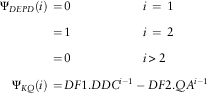 $$\hskip -50pt \eqalignno{ \Psi _{{DEPD}} (i)\,=\, & 0\quad \quad \quad \quad \quad \quad i\,=\,{\rm 1} \cr \,=\, & {\rm 1}\quad \quad \quad \quad \quad \quad i\,=\,{\rm 2} \cr \,=\, & 0\quad \quad \quad \quad \quad \quad i\,\gt\, {\rm 2} \cr \Psi _{{KQ}} (i)\,=\, & DF{\rm 1}.DDC^{i{-{\rm 1}}} -DF{\rm 2}.QA^{i{{\minus}{\rm 1}}} $$
where DF1=DW.DD/(1−QD), DF2=DF1.QD−DX and QD=QA/DDC
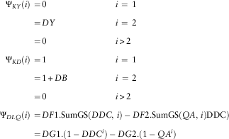 $$\eqalignno{ \Psi _{{KY}} (i)\,=\, & 0 \quad \quad \quad \quad \quad \quad \quad \quad i\,=\,{\rm 1} \cr \,=\, & DY\quad \quad \quad \quad \quad \quad \quad i\,=\,{\rm 2} \cr \,=\, & 0\quad \quad \quad \quad \quad \quad \quad \quad i\,\gt\, {\rm 2} \cr \Psi _{{KD}} (i)\,=\, & {\rm 1}\quad \quad \quad \quad \quad \quad \quad \quad i\,=\,{\rm 1} \cr \,=\, & {\rm 1}{\plus}DB\quad \quad \quad \quad \quad \,\,\,\,i\,=\,{\rm 2} \cr \,=\, & 0\quad \quad \quad \quad \quad \quad \quad \quad i\,\gt\, {\rm 2} \cr \Psi _{{DLQ}} (i)\,=\, & DF{\rm 1}.{\rm SumGS(}DDC,\,i{\rm )}-DF{\rm 2}.{\rm SumGS(}QA,\,i{\rm ) DDC}) \cr \,=\, & DG{\rm 1}.({\rm 1}-DDC^{i} )-DG{\rm 2}.({\rm 1}-QA^{i} ) $$
where DG1=DF1/(1−DDC) and DG2=DF2/(1−QA)
 $$\eqalignno{ \Psi _{{DLY}} (i)\,=\, & 0\quad \quad \quad \quad \quad \quad \quad \,i\,=\,{\rm 1} \cr \,=\, & DY^{i} \quad \quad \quad \quad \quad \quad i\,\gt\, {\rm 1} \cr \Psi _{{DLD}} (i)\,=\, & {\rm 1}\quad \quad \quad \quad \quad \quad \quad \,\,i\,=\,{\rm 1} \cr \,=\, & {\rm 1}{\plus}DB\quad \quad \quad \quad \quad i\,\gt\, {\rm 1} \cr \Psi _{{PLQ}} (i)\,=\, & \Psi _{{DLQ}} (i)-\Psi _{{YLQ}} (i) \cr \,=\, & DG{\rm 3}-DG{\rm 1}.DDC^{i} {\plus}DG{\rm 4}.QA^{i-{\rm 1}}} $$
where DG3=DG1−DG2 and DG4=DG2.QA−YW
 $$\eqalignno{ \Psi _{{PLY}} (i)\,=\, & \Psi _{{DLY}} (i)-\Psi _{{YLY}} (i) \cr \,=\, &-\!YA^{i{-{\rm 1}}} \quad \quad \quad \quad \quad \quad \quad i\,=\,{\rm 1} \cr \,=\, & DY-YA^{i{-{\rm 1}}} \quad \quad \quad \quad \quad \,i\,\gt\, {\rm 1} \cr \Psi _{{PLD}} (i)\,=\, & \Psi _{{DLD}} (i)-\Psi _{{YLD}} (i) \cr \,=\, & {\rm 1}\quad \quad \quad \quad \quad \quad \quad \quad \quad i\,=\,{\rm 1} \cr \,=\, & {\rm 1}{\plus}DB\quad \quad \quad \quad \quad \quad \quad i\,\gt\, {\rm 1} $$
A.3.6. Long-term interest rates
 $$\eqalignno{ \Psi _{{CMQ}} (i)\,=\, & CD.(CDC^{i} -QA^{i} )/(CDC-QA)\quad \quad \quad \quad \quad {\rm unless}\,CDC\,=\,QA \cr \Psi _{{CNC}} (i)\,=\, & CA^{i{-{\rm 1}}} \cr \Psi _{{CNY}} (i)\,=\, & CY.CA^{i{-{\rm 1}}} $$
A.3.7. Short-term interest rates
 $$\hskip -165pt \Psi _{{BDB}} (i)\,=\,BA^{i{-{\rm 1}}} $$
A.3.8. Index-linked rates
 $$\hskip -75pt \eqalignno{ & \Psi _{{RC}} (i)\,=\,RBC.RA^{i{-{\rm 1}}} \cr & \Psi _{{RR}} (i)\,=\,RA^{i{-{\rm 1}}} $$
A.4. Variances
A.4.1. The variances can be calculated by summing the squares of the Ψ-weights, or by direct calculation by the following formulae. The advantage of the formulae is that we can get precise expressions for the values as t→∞.
A.4.2. Inflation
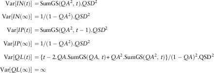 $$\eqalignno{ {\rm Var[}IN(t){\rm ]}\,=\, & {\rm SumGS(}QA^{{\rm 2}} ,\,t{\rm )}.QSD^{{\rm 2}} \cr {\rm Var[}IN(\infty){\rm ]}\,=\, & {\rm 1}/({\rm 1}-QA^{{\rm 2}} ).QSD^{{\rm 2}} \cr {\rm Var[}IP(t){\rm ]}\,=\, & {\rm SumGS(}QA^{{\rm 2}} ,\,t-{\rm 1)}.QSD^{{\rm 2}} \cr {\rm Var[}IP(\infty){\rm ]}\,=\, & {\rm 1}/({\rm 1}-QA^{{\rm 2}} ).QSD^{{\rm 2}} \cr {\rm Var[}QL(t){\rm ]}\,=\, & \{ t-{\rm 2}.QA.{\rm SumGS(}QA,\,t{\rm )}{\plus}QA^{{\rm 2}} .{\rm SumGS(}QA^{{\rm 2}} ,\,t{\rm )}\} /({\rm 1}-QA)^{{\rm 2}} .{\rm QSD}^{{\rm 2}} \cr {\rm Var[}QL(\infty){\rm ]}\,=\, & \infty $$
A.4.3. Wages
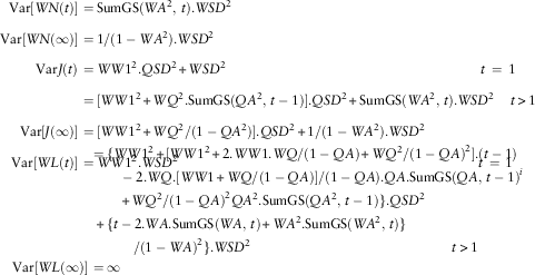 $$\eqalignno{ {\rm Var[}WN(t){\rm ]}\,=\, & {\rm SumGS(}WA^{{\rm 2}} ,\,t{\rm )}.WSD^{{\rm 2}} \cr {\rm Var[}WN(\infty){\rm ]}\,=\, & {\rm 1}/({\rm 1}-WA^{{\rm 2}} ).WSD^{{\rm 2}} \cr {\rm Var}J(t)\,=\, & WW1^{{\rm 2}} .QSD^{{\rm 2}} {\plus}WSD^{{\rm 2}} \quad \quad \quad \quad \quad \quad \quad \quad \quad \quad \quad \quad \quad \quad \quad \quad \quad \quad \quad t\,=\,{\rm 1} \cr \,=\, & [WW{\rm 1}^{{\rm 2}} {\plus}WQ^{{\rm 2}} .{\rm SumGS(}QA^{{\rm 2}} ,\,t-{\rm 1)}].QSD^{{\rm 2}} {\plus}{\rm SumGS(}WA^{{\rm 2}} ,\,t{\rm )}.WSD^{{\rm 2}} \quad \,t\,\gt\, {\rm 1} \cr {\rm Var[}J(\infty){\rm ]}\,=\, & [WW{\rm 1}^{{\rm 2}} {\plus}WQ^{{\rm 2}} /({\rm 1}-QA^{{\rm 2}} )].QSD^{{\rm 2}} {\plus}{\rm 1}/({\rm 1}-WA^{{\rm 2}} ).WSD^{{\rm 2}} \cr {\rm Var[}WL(t){\rm ]}\,=\, & WW{\rm 1}^{{\rm 2}} .WSD^{{\rm 2}} \quad \quad \quad \quad \quad \quad \quad \quad \quad \quad \quad \quad \quad \quad \quad \quad \quad \quad \quad \ \quad \quad \quad t\,=\,{\rm 1} \vskip-43pt \eqalign{ \,=\, & \{ WW{\rm 1}^{{\rm 2}} {\plus}[WW{\rm 1}^{{\rm 2}} {\plus}{\rm 2}.WW{\rm 1}.WQ/({\rm 1}-QA){\plus}WQ^{{\rm 2}} /({\rm 1 }-QA)^{{\rm 2}} ].(t-{\rm 1}) \cr & \quad -{\rm 2}.WQ.[WW{\rm 1}{\plus}WQ/({\rm 1}-QA)]/({\rm 1}-QA).QA.{\rm SumGS(}QA,\,t-{\rm 1)}^{i} \cr & \quad {\plus}WQ^{{\rm 2}} /({\rm 1}-QA)^{{\rm 2}} QA^{{\rm 2}} .{\rm SumGS(}QA^{{\rm 2}} ,\,t-{\rm 1)}\} .QSD^{{\rm 2}} \cr {\plus} & {\rm \{ }t-{\rm 2}.WA.{\rm SumGS(}WA,\,t{\rm )}{\plus}WA^{{\rm 2}} .{\rm SumGS}(WA^{{\rm 2}} ,\,t){\rm \} } \cr & \quad \quad /({\rm 1}-WA)^{{\rm 2}} \} .WSD^{{\rm 2}} \quad \quad \quad \quad \quad \quad \quad \quad \quad \quad \quad \quad \quad \quad \quad t\,\gt\, {\rm 1} \cr {\rm Var[}WL(\infty){\rm ]}\,=\, & \infty $$
A.4.4. Dividend yields
 $$\eqalignno{ {\rm Var[}YN(t){\rm ]}\,=\, & {\rm SumGS(}YA^{{\rm 2}} ,\,t{\rm )}.YSD^{{\rm 2}} \cr {\rm Var[}YN(\infty){\rm ]}\,=\, & {\rm 1}/({\rm 1}-YA^{{\rm 2}} ).YSD^{{\rm 2}} \cr {\rm Var[}YL(t){\rm ]}\,=\, & YW^{{\rm 2}} .{\rm SumGS(}QA^{{\rm 2}} ,\,t{\rm )}).QSD^{{\rm 2}} {\plus}{\rm SumGS(}YA^{{\rm 2}} ,\,t{\rm )}.YSD^{{\rm 2}} \cr {\rm Var[}YL(\infty){\rm ]}\,=\, & YW^{{\rm 2}} /({\rm 1}-QA^{{\rm 2}} ).QSD^{{\rm 2}} {\plus}{\rm 1}./({\rm 1}-YA^{{\rm 2}} ).YSD^{{\rm 2}} \cr {\rm Var[}YEP(t){\rm ]}\,=\, & 0\quad \quad \quad \quad \quad \quad \quad \quad \quad \quad \quad \quad \quad \quad \quad \quad \quad \quad \quad \quad \quad \quad t\,=\,{\rm 1} \cr \,=\, & YSD^{{\rm 2}} \quad \quad \quad \quad \quad \quad \quad \quad \quad \quad \quad \quad \quad \quad \quad \quad \ \,\ \quad \quad \quad \,\,t\,\gt\, {\rm 1} \cr {\rm Var[}YEP(\infty){\rm ]}\,=\, & YSD^{{\rm 2}} $$
A.4.5. Share dividends and prices
$$\eqalignno{ {\rm Var[}DM(t){\rm ]}\,=\, & \{ DD^{{\rm 2}} (DDC^{{\rm 2}} .{\rm SumGS(}DDC^{{\rm 2}} ,\,t{\rm )}-{\rm 2}.DDC.QA.{\rm SumGS(}DDC.QA,\,t{\rm )} \cr & {\plus}QA^{{\rm 2}} .{\rm SumGS(}QA^{{\rm 2}} ,\,t{\rm )})/(DDC-QA)^{{\rm 2}} \} .QSD^{{\rm 2}} \cr& {\rm unless}\,DDC\,=\,QA \cr {\rm Var[}DM(\infty){\rm ]}\,=\, & \{ DD^{{\rm 2}} \{ DDC^{{\rm 2}} /({\rm 1}-DDC^{{\rm 2}} )-{\rm 2}.QA\,DDC/({\rm 1}-QA\,DDC) \cr & {\plus}QA^{{\rm 2}} /({\rm 1}-QA^{{\rm 2}} )\} /(DDC-QA)^{{\rm 2}} \} .QSD^{{\rm 2}} \cr {\rm Var[}DEP(t){\rm ]}\,=\, & 0\qquad \quad \quad \quad \quad \quad \qquad \qquad \qquad \qquad \,\,t\,=\,{\rm 1} \cr \,=\, & DSD^{{\rm 2}} \quad \quad \quad \quad \quad \quad \quad \quad \quad \quad \quad \quad \quad \,\,t\,\gt\, {\rm 1} \cr {\rm Var[}DEP(\infty){\rm ]}\,=\, & DSD^{{\rm 2}} \cr {\rm Var[}K(t){\rm ]}\,=\, & (DW.DD{\plus}DX)^{{\rm 2}} .QSD^{{\rm 2}} {\plus}DSD^{{\rm 2}} \quad \quad \quad \quad \quad \quad t\,=\,{\rm 1} \cr \,=\, & \{ DF{\rm 1}^{{\rm 2}} .{\rm SumGS(}DDC^{{\rm 2}} ,\,t{\rm )}-{\rm 2}.DF{\rm 1}.DF{\rm 2}.{\rm SumGS(}DDC.QA,\,t{\rm )} \cr & {\plus}DF{\rm 2}^{{\rm 2}} .{\rm SumGS(}QA^{{\rm 2}} ,\,t{\rm )})\} .QSD^{{\rm 2}} {\plus}DY^{{\rm 2}} .YSD^{{\rm 2}} {\plus}({\rm 1}{\plus}DB^{{\rm 2}} ) \cdot DSD^{{\rm 2}} \cr & \qquad \qquad \qquad \qquad \qquad \quad \quad \quad \quad \quad \quad \quad \quad \quad \quad \,\,t\,\gt\, {\rm 1} \cr {\rm Var[}K(\infty){\rm ]}\,=\, & \{ DF{\rm 1}^{{\rm 2}} /({\rm 1}-DDC^{{\rm 2}} )-{\rm 2}.DF{\rm 1}.DF{\rm 2}/({\rm 1}-DDC.QA) \cr & {\plus}DF{\rm 2}^{{\rm 2}} /({\rm 1}-QA^{{\rm 2}} )\} .QSD^{{\rm 2}} {\plus}DY^{{\rm 2}} .YSD^{{\rm 2}} {\plus}({\rm 1}{\plus}DB^{{\rm 2}} ) \cdot DSD^{{\rm 2}} \vskip-38pt \eqalign{\cr {\rm Var[}DL(t){\rm ]}\,=\, & (DW.DD{\plus}DX)^{{\rm 2}} .QSD^{{\rm 2}} {\plus}DSD^{{\rm 2}} \quad \quad \quad \quad \quad \quad \quad \quad \quad \quad \qquad \quad t\,=\,{\rm 1} \cr \,=\, & \{ (DG{\rm 1}-DG{\rm 2})^{{\rm 2}} .t-{\rm 2}\,DG{\rm 1}.(DG{\rm 1}-DG{\rm 2})\,DDC.{\rm SumGS(}DDC,\,t{\rm )} \cr & {\plus}DG{\rm 1}^{{\rm 2}} \,DDC^{{\rm 2}} .{\rm SumGS(}DDC^{{\rm 2}} ,\,t{\rm )} \cr & -{\rm 2}.DG{\rm 1}.DG{\rm 2}.QA.DDC.{\rm SumGS(}QA.DDC,\,t{\rm )} \cr & {\plus}{\rm 2}DG{\rm 2}.(DG{\rm 1}-DG{\rm 2}).QA.{\rm SumGS(}QA,\,t{\rm )} \cr & {\plus}DG{\rm 2}^{{\rm 2}} .QA^{{\rm 2}} {\rm SumGS(}QA^{{\rm 2}} ,\,t{\rm )}\} .QSD^{{\rm 2}} \cr & {\plus} (t-{\rm 1}).DY^{{\rm 2}} YSD^{{\rm 2}} {\plus}\{ {\rm 1}{\plus}(t-{\rm 1}).({\rm 1}{\plus}DB)^{{\rm 2}} \} .DSD^{{\rm 2}} \quad \quad \quad \quad \quad t\,\gt\, {\rm 1} \cr \cr {\rm Var[}DL(\infty){\rm ]}\,=\, & \infty \cr \cr {\rm Var[}PL(t){\rm ]}\,=\, & (DW.DD{\plus}DX-YW)^{{\rm 2}} .QSD^{{\rm 2}} {\plus}YSD^{{\rm 2}} {\plus}DSD^{{\rm 2}} \quad \quad \quad \quad \quad \quad \quad t\,=\,{\rm 1} \cr \,=\, & \{ DG{\rm 3}^{{\rm 2}} .t{\plus}DG{\rm 1}^{{\rm 2}} .DDC^{{\rm 2}} .{\rm SumGS(}DDC^{{\rm 2}} ,\,t{\rm )} \cr & {\plus}DG{\rm 4}^{{\rm 2}} .{\rm SumGS(}QA^{{\rm 2}} ,\,t{\rm )} \cr & -{\rm 2}.DG{\rm 3}.DG{\rm 1}.DDC.{\rm SumGS(}DDC,\,t{\rm )} \cr & {\plus}{\rm 2}.DG{\rm 3}.DG{\rm 4}.{\rm SumGS(}QA,\,t{\rm )} \cr &-{\rm 2}.DG{\rm 1}.DG{\rm 4}.DDC.{\rm SumGS(}QA.DDC,\,t{\rm )}\} .QSD^{{\rm 2}} \cr & {\plus}\{ {\rm 1}{\plus}DY^{{\rm 2}} (t-{\rm 1})-{\rm 2}DY.YA.{\rm SumGS(}YA,\,t-{\rm 1)} \cr & {\plus}YA^{{\rm 2}} {\rm SumGS(}YA^{{\rm 2}} ,\,t-{\rm 1)}\} .YSD^{{\rm 2}} \cr & {\plus}\{ {\rm 1}{\plus}(t-{\rm 1}).({\rm 1}{\plus}DB)^{{\rm 2}} \} .DSD^{{\rm 2}} \qquad \qquad \qquad \qquad \qquad \qquad \qquad t\,\gt\, {\rm 1} \cr {\rm Var[}PL(\infty){\rm ]}\,=\, & \infty $$
A.4.6. Long-term interest rates
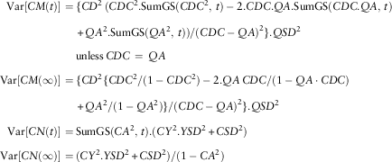 $$\eqalignno{ {\rm Var[}CM(t){\rm ]}\,=\, & \{ CD^{{\rm 2}} \,(CDC^{{\rm 2}} .{\rm SumGS(}CDC^{{\rm 2}} ,\,t{\rm )}-{\rm 2}.CDC.QA.{\rm SumGS(}CDC.QA,\,t{\rm )} \cr & {\plus}QA^{{\rm 2}} .{\rm SumGS(}QA^{{\rm 2}} ,\,t{\rm )})/(CDC-QA)^{{\rm 2}} \} .QSD^{{\rm 2}} \cr & {\rm unless}\,CDC\,=\,QA \cr {\rm Var[}CM(\infty){\rm ]}\,=\, & \{ CD^{{\rm 2}} \{ CDC^{{\rm 2}} /({\rm 1}-CDC^{{\rm 2}} )-{\rm 2}.QA\,CDC/({\rm 1}-QA \cdot CDC) \cr & {\plus}QA^{{\rm 2}} /({\rm 1}-QA^{{\rm 2}} )\} /(CDC-QA)^{{\rm 2}} \} .QSD^{{\rm 2}} \cr {\rm Var[}CN(t){\rm ]}\,=\, & {\rm SumGS(}CA^{{\rm 2}} ,\,t{\rm )}.(CY^{{\rm 2}} .YSD^{{\rm 2}} {\plus}CSD^{{\rm 2}} ) \cr {\rm Var[}CN(\infty){\rm ]}\,=\, & (CY^{{\rm 2}} .YSD^{{\rm 2}} {\plus}CSD^{{\rm 2}} )/({\rm 1}-CA^{{\rm 2}} ) $$
A.4.7. Short-term interest rates
 $$\hskip-80pt \eqalignno{ {\rm Var[}BDN(t){\rm ]}\,=\, & {\rm SumGS(}BA^{{\rm 2}} ,\,t{\rm )}.BSD^{{\rm 2}} \cr {\rm Var[}BDN(\infty){\rm ]}\,=\, & {\rm 1}/({\rm 1}-BA^{{\rm 2}} ).BSD^{{\rm 2}} $$
A.4.8. Index-linked rates
 $$\hskip-50pt \eqalignno{ {\rm Var[}RN(t){\rm ]}\,=\, & (RBC^{{\rm 2}} .CSD^{{\rm 2}} {\plus}RSD^{{\rm 2}} \,{\rm SumGS(}RA,\,t{\rm )} \cr {\rm Var[}RN{\rm (}\infty{\rm )]}\,=\, & (RBC^{{\rm 2}} .CSD^{{\rm 2}} {\plus}RSD^{{\rm 2}} )/({\rm 1}-RA^{{\rm 2}} ) $$
A.5. Covariances
A.5.1. Like the variances, the covariances can be calculated by summing the cross-products of the Ψ-weights, or by direct calculation by the following formulae. Again, the advantage of the formulae is that we can get precise expressions for the values as t→∞. A covariance exists wherever two variables are dependent on the common innovations; other covariances are zero, and are omitted below.
A.5.2. Inflation
 $$\eqalignno{ {\rm Covar[}IN(t),\,IP(t){\rm ]}\,=\, & QA.{\rm SumGS(}QA^{{\rm 2}} ,\,t{\rm )}.QSD^{{\rm 2}} \cr {\rm Covar[}IN(\infty),\,IP(\infty){\rm ]}\,=\, & QA/({\rm 1}-QA^{{\rm 2}} ).QSD^{{\rm 2}} $$
As the formulae are very simple we can calculate the correlation coefficients, which are:
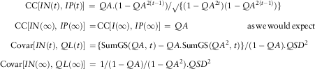 $$\eqalignno{ & {\rm \hskip-85pt CC[}IN(t),\,IP(t){\rm ]}\,=\, QA.({\rm 1}-QA^{{{\rm 2}(t{\minus}{\rm 1})}} )/\surd\{ ({\rm 1}-QA^{{{\rm 2}t}} )({\rm 1}-QA^{{{\rm 2}(t-{\rm 1})}} )\} \cr \qquad {\rm CC[}IN(\infty),\,IP(\infty){\rm ]}\,=\, & {\rm CC[}I(\infty),\,IP(\infty){\rm ]}\,=\,QA\quad \quad \quad \quad \quad \quad \quad {\rm as}\,{\rm we}\,{\rm would}\,{\rm expect} \cr {\rm Covar[}IN(t),\,QL(t){\rm ]}\,=\, & \{ {\rm SumGS(}QA,\,t{\rm )}-QA.{\rm SumGS(}QA^{{\rm 2}} ,\,t{\rm )}\} /({\rm 1}-QA).QSD^{{\rm 2}} \cr {\rm \hskip-115pt Covar[}IN(\infty),\,QL(\infty){\rm ]}\,=\,{\rm 1}/({\rm 1}-QA)/({\rm 1}-QA^{{\rm 2}} ).QSD^{{\rm 2}} $$
But as Var[QL(∞)}]→∞ as t→∞, CC[I(∞), QL(∞)]→0. In the very long run, there is no correlation between the value of inflation in any year and the value of the price index in the same year, although in the first year the correlation is unity:
 $$\eqalignno{ {\rm Covar[}IP(t),\,QL(t){\rm ]}\,=\, & \{ {\rm SumGS(}QA,\,t-1{\rm )}-QA^{{\rm 2}} .{\rm SumGS(}QA^{{\rm 2}} ,\,t-{\rm 1)}\} /({\rm 1}-QA).QSD^{{\rm 2}} \cr {\rm Covar[}IP(\infty),\,QL(\infty){\rm ]}\,=\, & \{ {\rm 1}-QA^{{\rm 2}} /({\rm 1}{\plus}QA)\} /({\rm 1}-QA)^{{\rm 2}} .QSD^{{\rm 2}} $$
A.5.3. Wages
$$\eqalignno{ {\rm Covar[}IN(t),\,J(t){\rm ]}\,=\, & \{ WW{\rm 1}{\plus}WQ.QA.{\rm SumGS(}QA^{{\rm 2}} ,\,t-{\rm 1)}\} .QSD^{{\rm 2}} \cr {\rm Covar[}IN(\infty),\,J(\infty){\rm ]}\,=\, & \{ WW{\rm 1}{\plus}WQ.QA/({\rm 1}-QA^{{\rm 2}} )\} .QSD^{{\rm 2}} \cr {\rm Covar[}IP(t),\,J(t){\rm ]}\,=\, & 0\quad \qquad \qquad \qquad \qquad \qquad \qquad \qquad \qquad \qquad \quad \quad t\,=\,{\rm 1} \cr\,=\, & WQ.{\rm SumGS(}QA^{{\rm 2}} ,\,t-{\rm 1)}.QSD^{{\rm 2}} \qquad \qquad \quad \ \ \qquad t\,\gt\, {\rm 1} \cr {\rm Covar[}IP(\infty),\,J(\infty){\rm ]}\,=\, & WQ/({\rm 1}-QA^{{\rm 2}} ).QSD^{{\rm 2}} \cr {\rm Covar[}QL(t),\,J(t){\rm ]}\,=\, & [WW{\rm 1}{\plus}WQ.\{ {\rm SumGS(}QA,\,t-{\rm 1)}-QA^{{\rm 2}} .{\rm SumGS(}QA^{{\rm 2}} ,\,t-{\rm 1)}\} \cr & \quad \quad \quad \,\,/({\rm 1}-QA)].QSD^{{\rm 2}}\openup2.5pt \vskip-43pt \eqalign{\cr {\rm Covar[}QL(\infty),\,J(\infty){\rm ]}\,=\, & [WW{\rm 1}{\plus}WQ.\{ {\rm 1}/({\rm 1}-QA)-QA^{{\rm 2}} /({\rm 1}-QA^{{\rm 2}} )\} /({\rm 1}-QA)].QSD^{{\rm 2}} \cr {\rm Covar[}WN(t),\,J(t){\rm ]}\,=\, & {\rm SumGS(}WA^{{\rm 2}} ,\,t{\rm )}.WSD^{{\rm 2}} \cr {\rm Covar[}WN(\infty),\,J(\infty){\rm ]}\,=\, & {\rm 1}/({\rm 1}-WA^{{\rm 2}} ).WSD^{{\rm 2}} \cr {\rm Covar[}IN(t),\,WL(t){\rm ]}\,=\, & WW{\rm 1}.QSD^{{\rm 2}} \qquad \qquad \quad \qquad \quad \quad \quad \quad \quad \quad \quad \quad \quad \quad \quad \quad \quad \quad \quad t\,=\,{\rm 1} \cr \,=\, & \{ WW{\rm 1}{\plus}(WW{\rm 1}{\plus}WQ/({\rm 1}-QA)).QA.{\rm SumGS(}QA,\,t-{\rm 1)} \cr & -WQ/({\rm 1}-QA).QA^{{\rm 2}} .{\rm SumGS(}QA^{{\rm 2}} ,\,t-{\rm 1)}\} .QSD^{{\rm 2}} \qquad \quad \quad \quad t\,\gt\, {\rm 1} \cr {\rm Covar[}IN(\infty),\,WL(\infty){\rm ]}\,=\, & \{ WW{\rm 1}{\plus}(WW{\rm 1}{\plus}WQ/({\rm 1}-QA)).QA/({\rm 1}-QA) \cr & -WQ/({\rm 1}-QA).QA^{{\rm 2}} /({\rm 1}-QA^{{\rm 2}} )\} .QSD^{{\rm 2}} \cr {\rm Covar[}IP(t),\,WL(t){\rm ]}\,=\, & 0\quad \quad \quad \quad \quad \qquad \qquad \quad \quad \quad \quad \quad \quad \quad \quad \quad \quad \quad \quad \quad \quad \quad \quad \quad \quad t\,=\,{\rm 1} \cr \,=\, & \{ (WW{\rm 1}{\plus}WQ/({\rm 1}-QA)).{\rm SumGS(}QA,\,t-{\rm 1)} \cr & -WQ/({\rm 1}-QA).QA.{\rm SumGS(}QA^{{\rm 2}} \,t-{\rm 1)}\} .QSD^{{\rm 2}} \quad \qquad \ \ \quad \ \quad t\,\gt\, {\rm 1} \cr {\rm Covar[}IP(\infty),\,WL(\infty){\rm ]}\,=\, & {\rm }\{ (WW{\rm 1}{\plus}WQ/({\rm 1}-QA))/({\rm 1}-QA) \cr & -WQ/({\rm 1}-QA).QA/({\rm 1}-QA^{{\rm 2}} )\} .QSD^{{\rm 2}} \cr \hskip-162pt {\rm Covar[}QL(t),\,WL(t){\rm ]}\,=\, & WW{\rm 1}.QSD^{{\rm 2}} \quad \quad \quad \qquad \qquad \qquad \qquad \qquad \qquad \qquad \quad \qquad \quad \quad t\,=\,{\rm 1} \cr \,=\, & WW{\rm 1}.QSD^{{\rm 2}} \cr & {\plus}\{ \{ (WW{\rm 1}{\plus}WQ/({\rm 1}-QA)).(t-{\rm 1}) \cr & - (WW{\rm 1}{\plus}WQ/({\rm 1}-QA)).QA.(QA{\plus}{\rm 1}).{\rm SumGS(}QA,\,t-{\rm 1)} \cr &{\plus} WQ/({\rm 1}-QA).QA^{{\rm 3}} .{\rm SumGS(}QA^{{\rm 2}}\!\!\!\! \!t-{\rm 1)}\} /({\rm 1}-QA).QSD^{{{\rm 2} }} \quad \quad \quad t\,\gt\, {\rm 1} \cr {\rm Covar[}QL(\infty),\,WL(\infty){\rm ]}\,=\, & \infty \cr {\rm Covar[}WN(t),\,WL(t){\rm ]}\,=\, & \{ {\rm SumGS(}WA,\,t{\rm )}-WA.{\rm SumGS(}WA^{{\rm 2}} ,\,t{\rm )})/({\rm 1}-WA)\} .WSD^{{\rm 2}} \cr {\rm Covar[}WN(\infty),\,WL(\infty){\rm ]}\,=\, & \{ {\rm 1}/({\rm 1}-WA)-WA/({\rm 1}-WA^{{\rm 2}} ))/({\rm 1}-WA).WSD^{{\rm 2}} \cr {\rm Covar[}J(t),\,WL(t){\rm ]}\,=\, & WW{\rm 1}^{{\rm 2}} .QSD^{{\rm 2}} {\plus}\quad \qquad \qquad \qquad \qquad \qquad \quad \quad \quad \quad \quad \quad \quad \quad \quad \quad t\,=\,{\rm 1} \cr \,=\, & [WW{\rm 1}^{{\rm 2}} {\plus}\{ WQ.(WW{\rm 1}{\plus}WQ/({\rm 1}-QA)){\rm }.{\rm SumGS(}QA,\,t-{\rm 1)} \cr & - WQ^{{\rm 2}} /({\rm 1}-QA).QA.{\rm SumGS(}QA^{{\rm 2}} \,t-{\rm 1)}\} ].QSD^{{\rm 2}} \cr & {\plus} \{ ({\rm SumGS(}WA,\,t{\rm ) }-WA^{{\rm 2}} .{\rm SumGS(}WA^{{\rm 2}} ,\,t{\rm )}\} /({\rm 1}-WA).WSD^{{\rm 2}} \quad t\,\gt\, {\rm 1} \cr {\rm Covar[}J(\infty),\,WL(\infty \ t {\rm ]\,=\,} & [WW{\rm 1}^{{\rm 2}} {\plus}\{ WQ.{\rm (}WW{\rm 1}{\plus}WQ/({\rm 1}-QA){\rm )}/({\rm 1}-QA) \cr & -WQ^{{\rm 2}} /({\rm 1}-QA).QA/({\rm 1}-QA^{{\rm 2}} )\} .QSD^{{\rm 2}} \cr & {\plus} \{ {\rm 1}/({\rm 1}-WA)-WA/({\rm 1}-WA^{{\rm 2}} )\} /({\rm 1}-WA)\} .WSD^{{\rm 2}} $$
A.5.4. Dividend yields
$$\eqalignno{ {\rm Covar(}IN(t),\,YL(t){\rm )}\,=\, & YW.{\rm SumGS(}QA^{{\rm 2}} ,\,t{\rm )}.QSD^{{\rm 2}} \cr {\rm Covar(}IN(\infty),\,YL(\infty){\rm )}\,=\, & YW/({\rm 1}-QA^{{\rm 2}} ).QSD^{{\rm 2}} \cr {\rm Covar(}IP(t),\,YL(t){\rm )}\,=\, & 0\quad \quad \quad \quad \quad \quad \quad \quad \quad \quad \quad \quad \quad \qquad \qquad \qquad \quad \qquad t\,=\,{\rm 1} \cr \,=\, & YW.QA.{\rm SumGS(}QA^{{\rm 2}} ,\,t-{\rm 1)}.QSD^{{\rm 2}} \qquad \qquad \quad \quad \quad t\,\gt\, {\rm 1} \vskip-35pt \eqalign{\cr {\rm Covar(}IP(\infty),\,YL(\infty){\rm )}\,=\, & YW.QA/({\rm 1}-QA^{{\rm 2}} ).QSD^{{\rm 2}} \cr {\rm Covar(}QL(t),\,YL(t){\rm )}\,=\, & YW/({\rm 1}-QA)\{ {\rm SumGS(}QA,\,t{\rm )}-QA.{\rm SumGS(}QA^{{\rm 2}} ,\,t{\rm )}\} .QSD^{{\rm 2}} \cr {\rm Covar(}QL(\infty),\,YL(\infty){\rm )}\,=\, & YW/\{ ({\rm 1}-QA).{\rm (1}-QA^{{\rm 2}} {\rm )}\} .QSD^{{\rm 2}} \cr {\rm Covar(}J(t),\,YL(t){\rm )}\,=\, & WW{\rm 1}.YW.QSD^{{\rm 2}} \quad \quad \quad \quad \quad \quad \ \ \qquad \qquad \quad \quad \quad \quad \quad t\,=\,{\rm 1} \cr \,=\, & YW.\{ WW{\rm 1}{\plus}WQ.QA.{\rm SumGS(}QA^{{\rm 2}} ,\,t-{\rm 1)}\} .QSD^{{\rm 2}} \quad t\,\gt\, {\rm 1} \cr \cr {\rm Covar(}J(\infty),\,YL(\infty){\rm )}\,=\, & YW.\{ WW{\rm 1}{\plus}WQ.QA/({\rm 1}-QA^{{\rm 2}} )\} .QSD^{{\rm 2}} \cr {\rm Covar(}WL(t),\,YL(t){\rm )}\,=\, & WW{\rm 1}.YW.QSD^{{\rm 2}} \quad \quad \quad \quad \quad \quad \quad \quad \quad \qquad \quad \qquad \quad \,\,t\,=\,{\rm 1} \cr \,=\, & YW.\{ WW{\rm 1}{\plus}(WW{\rm 1}{\plus}WQ/({\rm 1}-QA)).QA.{\rm SumGS(}QA,\,t-{\rm 1)} \cr & - WQ/({\rm 1}-QA).QA^{{\rm 2}} .{\rm SumGS}(QA^{{\rm 2}} ,\,t-{\rm 1}\} .QSD^{{\rm 2}} \quad \quad \,\,t\,\gt\, {\rm 1} \cr \cr {\rm Covar(}WL(\infty),\,YL(\infty){\rm )}\,=\, & YW.\{ WW{\rm 1}{\plus}(WW{\rm 1}{\plus}WQ/({\rm 1}-QA^{{\rm 2}} )).QA/({\rm 1}-QA)\} .QSD^{{\rm 2}} \cr {\rm Covar(}YN(t),\,YL(t){\rm )}\,=\, & {\rm SumGS(}YA^{{\rm 2}} ,\,t{\rm )}.YSD^{{\rm 2}} \,=\,{\rm Var[}YN(t){\rm ]} \cr {\rm Covar(}YN(\infty),\,YL(\infty){\rm )}\,=\, & {\rm 1}/({\rm 1}-YA^{{\rm 2}} ).YSD^{{\rm 2}} \cr {\rm Covar(}YL(t),\,YEP(t){\rm )}\,= & 0\quad \quad \quad \quad \qquad\qquad\qquad\qquad\qquad\qquad\quad \,\,t\,=\,{\rm 1}\,\ {\rm or}\ \,t\,\gt\, {\rm 2} \cr = & YA.YSD^{{\rm 2}} \qquad\qquad\qquad\qquad\qquad\qquad\quad\quad t\,=\,{\rm 2} \cr {\rm Covar(}YL(\infty),\,YEP(\infty){\rm )}\,=\, & 0 $$
A.5.5. Share dividends and prices
$$\eqalignno{ {\rm Covar(}IN(t),\,DM(t){\rm )}\,=\, & DD/(DDC-QA) \cr & .\{ DDC.{\rm SumGS(}QA.DDC,\,t{\rm )}-QA.{\rm SumGS(}QA^{{\rm 2}} ,\,t{\rm )}\} .QSD^{{\rm 2}} \cr {\rm Covar(}IN(\infty),\,DM(\infty){\rm )}\,=\, & DD/(DDC-QA) \cr& .\{ DDC/({\rm 1}-QA.DDC)-QA/({\rm 1 }-QA^{{\rm 2}} )\} .QSD^{{\rm 2}} \cr {\rm Covar(}IP(t),\,DM(t){\rm )}\,=\, & 0\qquad \qquad \qquad \qquad \qquad \qquad \qquad \qquad \qquad t\,=\,{\rm 1} \cr \,=\, & DD/(DDC-QA).\{ DDC^{{\rm 2}} .{\rm SumGS(}QA.DD,\,t-{\rm 1)} \cr &-QA^{{\rm 2}} .{\rm SumGS(}QA^{{\rm 2}} ,\,t-{\rm 1)}\} .QSD^{{\rm 2}} \quad \quad \,\,t\,\gt\, {\rm 1} \cr {\rm Covar(}IP(\infty),\,DM(\infty){\rm )}\,=\, & DD/(DDC-QA)\{ {\rm 1}/({\rm 1}-QA.DDC)-QA^{{\rm 2}} /({\rm 1}-QA^{{\rm 2}} )\} .QSD^{{\rm 2}} \cr {\rm Covar(}QL(t),\,DM(t){\rm )}\,=\, & DD/\{ ({\rm 1 }-QA).(DDC-QA)\} \cr & .\{ DDC.{\rm SumGS(}DDC,\,t{\rm )}-QA.{\rm SumGS(}QA,\,t{\rm )} \cr & -QA.DDC.{\rm SumGS(}QA.DDC,\,t{\rm )}{\plus}QA^{{\rm 2}} .{\rm SumGS(}QA^{{\rm 2}} ,\,t{\rm )}).QSD^{{\rm 2}} \cr {\rm Covar(}QL(\infty),\,DM(\infty){\rm )}\,=\, & DD/\left\{ {({\rm 1}-QA).(DDC-QA)} \right\} \cr & .\{ DDC/({\rm 1}-DDC)-QA/({\rm 1}-QA) \cr & -QADDC/({\rm 1}-QA.DDC){\plus}QA^{{\rm 2}} /({\rm 1}-QA^{{\rm 2}} )\} .QSD^{{\rm 2}} $$
$$\hskip-32pt \eqalignno{ \vskip 10pt \eqalign{{\cr \cr \rm Covar(}J(t),\,DM(t){\rm )}\,=\, & WW{\rm 1}.DD.QSD^{{\rm 2}} \quad \quad \quad \quad \quad \quad \quad \quad \quad t\,=\,{\rm 1} \cr \,=\, & [WW{\rm 1}.DD{\plus}WQ.DD/(DDC-QA) \cr & \hskip-2pt .\{ DDC^{{\rm 2}} .{\rm SumGS(}QA.DDC,\,t-{\rm 1)}-QA^{{\rm 2}} .{\rm SumGS(}QA^{{\rm 2}} ,\,t-{\rm 1)}\} ].QSD^{{\rm 2}} \cr & \qquad \qquad \qquad \qquad \qquad \qquad \qquad \qquad \qquad \qquad \qquad \qquad \qquad t\,\gt\, {\rm 1} \cr {\rm Covar(}J(\infty),\,DM(\infty){\rm )}\,=\, & [WW{\rm 1}.DD{\plus}WQ.DD/(DDC-QA) \cr & .\{ DDC^{{\rm 2}} /({\rm 1}-QA.DDC)-QA^{{\rm 2}} /({\rm 1}-QA^{{\rm 2}} )\} ].QSD^{{\rm 2}} \cr {\rm Covar(}WL(t),\,DM(t){\rm )}\,=\, & WW{\rm 1}.DD.QSD^{{\rm 2}} \quad \quad \quad \quad \quad \quad \,\,t\,=\,{\rm 1} \cr \,=\,& [WW{\rm 1}.DD{\plus}DD/(DDC-QA) \cr & . \{ (WW{\rm 1}{\plus}WQ/({\rm 1}-QA)) \cr & .(DDC^{{\rm 2}} .{\rm SumGS(}DDC,\,t-{\rm 1)}-QA^{{\rm 2}} {\rm SumGS(}QA,\,t-{\rm 1)}) \cr & -WQ/({\rm 1}-QA).QA. \cr & (DDC^{{\rm 2}} .{\rm SumGS(}QA.DDC,\,t-{\rm 1)}{\plus}QA^{{\rm 2}} .{\rm SumGS(}QA^{{\rm 2}} ,\,t-{\rm 1)})\} ].QSD^{{\rm 2}} \cr & \qquad \qquad \qquad \qquad \qquad \qquad \qquad \qquad \qquad \qquad \qquad \qquad \qquad \,\,\,t\,\gt\, {\rm 1} \cr {\rm Covar(}WL(\infty),\,DM(\infty){\rm )}\,=\, & [WW{\rm 1}.DD{\plus}DD/(DDC-QA) \cr .\{ (WW{\rm 1}{\plus}QA/({\rm 1}-QA).(DDC^{{\rm 2}} /({\rm 1}-DDC)-QA^{{\rm 2}} /({\rm 1}-QA)) \cr -WQ/({\rm 1}-QA).QA.[DDC^{{\rm 2}} /({\rm 1}-DDC)-QA^{{\rm 2}} /({\rm 1}-QA^{{\rm 2}} )\} .QSD^{{\rm 2}} $$
$$\eqalignno{ {\rm Covar(}YL(t),\,DM(t){\rm )}\,=\, & YW.DD/(DDC-QA) \cr & \quad .\{ DDC.{\rm SumGS(}DDC.QA,t{\rm )}-QA.{\rm SumGS(}QA^{{\rm 2}} ,\,t{\rm )}\} .QSD^{{\rm 2}} \cr {\rm Covar(}YL(\infty),\,DM(\infty){\rm )}\,=\, & YW.DD/(DDC-QA) \cr .\{ DDC/({\rm 1}-DDC.QA)-QA/({\rm 1}-QA^{{\rm 2}} )\} .QSD^{{\rm 2}} \cr {\rm Covar(}IN(t),\,K(t){\rm )}\,=\, & \{ DF{\rm 1}.{\rm SumGS(}QA.DDC,\,t{\rm )}-DF{\rm 2}.{\rm SumGS(}QA^{{\rm 2}} ,\,t{\rm )}\} .QSD^{{\rm 2}} \cr {\rm Covar(}IN(\infty),\,K(\infty){\rm )}\,=\, & \{ DF{\rm 1}/({\rm 1}-QA.DDC)-DF{\rm 2}/({\rm 1}-QA^{{\rm 2}} )\} .QSD^{{\rm 2}} \cr {\rm Covar(}IP(t),\,K(t){\rm )}\,=\, & \{ DF{\rm 1}.DDC.{\rm SumGS(}QA.DDC,\,t{\rm )}-DF{\rm 2}.QA.{\rm SumGS(}QA^{{\rm 2}} ,\,t{\rm )}\} .QSD^{{\rm 2}} \cr {\rm Covar(}IP(\infty),\,K(\infty){\rm )}\,=\, & \{ DF{\rm 1}.DDC/({\rm 1}-QA.DDC)-DF{\rm 2}.QA/({\rm 1}-QA^{{\rm 2}} )\} .QSD^{{\rm 2}} \cr {\rm Covar(}QL(t),\,K(t){\rm )}\,=\, & \{ DF{\rm 1}.{\rm SumGS(}DDC,\,t{\rm )}-DF{\rm 1}.QA.{\rm SumGS(}DDC.QA,\,t{\rm )} \cr & - DF{\rm 2}.{\rm SumGS(}QA,\,t{\rm )}{\plus}DF{\rm 2}.QA.{\rm SumGS(}QA^{{\rm 2}} ,\,t{\rm )}\} /({\rm 1}-QA).QSD^{{\rm 2}} \cr {\rm Covar(}QL(\infty),\,K(\infty){\rm )}\,=\, & \{ DF{\rm 1}/({\rm 1}-DDC)-DF{\rm 1}.QA/({\rm 1}-DDC.QA) \cr & - DF{\rm 2}/({\rm 1}-QA){\plus}DF{\rm 2}.QA/({\rm 1}-QA^{{\rm 2}} )\} /({\rm 1}-QA).QSD^{{\rm 2}} \cr {\rm Covar(}J(t),\,K(t){\rm )}\,=\, & WW{\rm 1}.(DW.DD{\plus}DX).QSD^{{\rm 2}} \quad \quad \quad \quad \quad \quad \quad \quad \quad \quad t\,=\,{\rm 1} \cr \,=\, & [WW{\rm 1}.(DW.DD{\plus}DX) \cr & {\plus}\{ WQ.(DF{\rm 1}.DDC.{\rm SumGS(}QA.DDC,\,t-{\rm 1)} \cr & -DF{\rm 2}.QA.{\rm SumGS(}QA^{{\rm 2}} ,\,t-{\rm 1)})\} ].QSD^{{\rm 2}} \quad \qquad \qquad \quad t\,\gt\, {\rm 1} \cr {\rm Covar(}J(\infty),\,K(\infty){\rm )}\,=\, & [WW{\rm 1}.(DW.DD{\plus}DX) \cr & {\plus} \{ WQ.(DF{\rm 1}.DDC/({\rm 1}-QA.DDC)-DF{\rm 2}.QA/({\rm 1}-QA^{{\rm 2}} ))\} ].QSD^{{\rm 2}} $$
$$\hskip-5pt \eqalignno{ {\rm Covar(}WL(t),\,K(t){\rm )}\,=\, & WW{\rm 1}.(DW.DD{\plus}DX).QSD^{{\rm 2}} \quad \quad \quad \quad \quad \quad t\,=\,{\rm 1} \cr \,=\, & [WW{\rm 1}.(DW.DD{\plus}DX) \cr & {\plus} \{ WW{\rm 1}.(DF{\rm 1}.DDC.{\rm SumGS(}DDC,\,t-{\rm 1)}-DF{\rm 2}.QA.{\rm SumGS(}QA,\,t-{\rm 1)}) \cr & {\plus} WQ/({\rm 1}-QA).[DF{\rm 1}.DDC.({\rm SumGS(}DDC,\,t-{\rm 1)}-QA.{\rm SumGS(}DDC.QA,\,t-{\rm 1)}) \cr & -DF{\rm 2}.QA.({\rm SumGS(}QA,\,t-{\rm 1)}-QA.{\rm SumGS(}QA^{{\rm 2}} ,\,t-{\rm 1)})\left] \} \right].QSD^{{\rm 2}} \cr {\rm Covar(}WL(\infty),\,K(\infty){\rm )}\,=\, & [WW{\rm 1}.(DW.DD{\plus}DX) \cr & {\plus} \{ WW{\rm 1}.(DF{\rm 1}.DDC/({\rm 1}-DDC)-DF{\rm 2}.QA/({\rm 1}-QA)] \cr & {\plus} WQ/({\rm 1}-QA).[DF{\rm 1}.DDC/({\rm 1}-DDC)-DF{\rm 1}.DDC.QA/({\rm 1}-DDC.QA) \cr & -DF{\rm 2}.QA.({\rm 1}/({\rm 1}-QA)-QA/({\rm 1}-QA^{{\rm 2}} ))]\} ].QSD^{{\rm 2}} \cr {\rm Covar(}YN(t),\,K(t){\rm )}\,=\, & 0\quad \quad \quad \quad \quad \quad \quad \quad \quad \quad \quad \quad \quad \quad \quad \quad t\,=\,{\rm 1} \cr \,=\, & YA.DY.YSD^{{\rm 2}} \quad \quad \quad \quad \quad \quad \quad \quad \quad \quad \quad \,\,t\,\gt\, {\rm 1} \cr {\rm Covar(}YN(\infty),\,K(\infty){\rm )}\,=\, & YA.DY.YSD^{{\rm 2}} \cr {\rm Covar(}YEP(t),\,K(t){\rm )}\,=\, & 0\quad \quad \quad \quad \quad \quad \quad \quad \quad \quad \quad \quad \quad \quad \quad \quad t\,=\,{\rm 1} \cr \,=\, & DY.YSD^{{\rm 2}} \quad \quad \quad \quad \quad \quad \quad \quad \quad \quad \quad \quad \,\,\,t\,\gt\, {\rm 1} \cr {\rm Covar(}YEP(\infty),\,K(\infty){\rm )}\,=\, & DY.YSD^{{\rm 2}} \cr {\rm Covar(}YL(t),\,K(t){\rm )}\,=\, & \{ YW.[DF{\rm 1}.{\rm SumGS(}DDC.QA,\,t{\rm )}-DF{\rm 2}.{\rm SumGS(}QA^{{\rm 2}} ,\,t{\rm )}]\} .QSD^{{\rm 2}} \quad t\,=\,{\rm 1} \cr \,=\, & \{ YW.[DF{\rm 1}.{\rm SumGS(}DDC.QA,\,t{\rm )}-DF{\rm 2}.{\rm SumGS(}QA^{{\rm 2}} ,\,t{\rm )}]\} .QSD^{{\rm 2}} \cr & {\plus}YA.DY.YSD^{{\rm 2}} \quad \quad \quad \quad \quad \quad \quad \quad \quad \quad \quad \quad \quad \quad \quad \quad \quad \quad \,\,\,t\,\gt\, {\rm 1} \cr {\rm Covar(}YL(\infty),\,K(\infty){\rm )}\,=\, & \{ YW.[DF{\rm 1}/({\rm 1}-DDC.QA)-DF{\rm 2}/({\rm 1}-QA^{{\rm 2}} )]\} .QSD^{{\rm 2}} \cr & {\plus}YA.DY.YSD^{{\rm 2}} $$
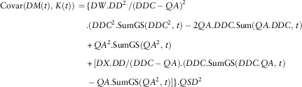 $$\eqalignno{ {\rm Covar(}DM(t),\,K(t){\rm )}\,=\, & \{ DW.DD^{{{\rm 2}{\rm .}}} /(DDC-QA)^{{\rm 2}} \cr & . (DDC^{{\rm 2}} .{\rm SumGS(}DDC^{{\rm 2}} ,\,t{\rm )}-{\rm 2}QA.DDC.{\rm Sum(}QA.DDC,\,t{\rm )} \cr & {\plus}QA^{{\rm 2}} .{\rm SumGS(}QA^{{\rm 2}} ,\,t{\rm )} \cr & {\plus}{\rm }[DX.DD/(DDC-QA).(DDC.{\rm SumGS(}DDC.QA,\,t{\rm )} \cr & -QA.{\rm SumGS}(QA^{{\rm 2}} ,\,t)]\} .QSD^{{\rm 2}} $$
 $$\eqalignno{ {\rm Covar(}DM(\infty),\,K(\infty){\rm )}\,=\, & \{ DW.[DD^{{{\rm 2}}} /(DDC-QA)^{{\rm 2}} \cr & . (DDC^{{{\rm 2}/}} /({\rm 1}-DDC^{{\rm 2}} )-{\rm 2}QA.DDC/({\rm 1}-QA.DDC) \cr & {\plus}QA^{{\rm 2}} /({\rm 1}-QA^{{\rm 2}} )) \cr & {\plus} [DX.DD/(DDC-QA).(DDC/({\rm 1}-DDC.QA) \cr & -QA/({\rm 1}-QA^{{\rm 2}} )]\} .QSD^{{\rm 2}} $$
 $$\vskip 2.2pt\eqalignno{ {\rm Covar(}DEP(t),\,K(t){\rm )}\,=\, & 0\quad \quad \quad \quad \quad \quad \quad \quad t\,=\,{\rm 1} \cr \,=\, & DB.DSD^{{\rm 2}} \quad \quad \quad \quad \,\,t\,\gt\, {\rm 1} $$
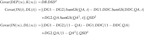 $$\eqalignno{ \cr{\rm Covar(}DEP(\infty),K(\infty){\rm )}\,=\, & DB.DSD^{{\rm 2}} \cr {\rm Covar(}IN(t),DL(t){\rm )}\,=\, & [(DG{\rm 1}-DG{\rm 2}).{\rm SumGS(}QA,\,t{\rm )}-DG{\rm 1}.DDC.{\rm SumGS(}DDC.QA,\,t{\rm )} \cr & {\plus}DG{\rm 2}.QA.{\rm SumGS(}QA^{{\rm 2}} ,\,t{\rm )}].QSD^{{\rm 2}} \cr {\rm Covar(}IN(\infty),DL(\infty){\rm )}\,=\, & [(DG{\rm 1}-DG{\rm 2})/({\rm 1}-QA)-DG{\rm 1}.DDC/({\rm 1}-DDC.QA) \cr & {\plus}DG{\rm 2}.QA/({\rm 1}-QA^{{\rm 2}} )].QSD^{2} $$
 $$\eqalignno{ {\rm Covar(}IP(t),DL(t){\rm )}\,=\, & 0\qquad \qquad \qquad \qquad \qquad \qquad \qquad \qquad \qquad \qquad \qquad \qquad \qquad t\,=\,{\rm 1} \cr \,=\, & [(DG{\rm 1}-DG{\rm 2}).{\rm SumGS(}QA,\,t-{\rm 1)}-DG{\rm 1}.DDC^{{\rm 2}} .{\rm SumGS(}QA.DDC,\,t-{\rm 1)} \cr & {\plus}DG{\rm 2}.QA^{{\rm 2}} .{\rm SumGS(}QA^{{\rm 2}} ,\,t-{\rm 1)}].QSD^{{\rm 2}} $$
 $$\eqalignno{ {\rm Covar(}IP(\infty),DL(\infty){\rm )}\,=\, & [(DG{\rm 1}-DG{\rm 2})/({\rm 1}-QA)-DG{\rm 1}.DDC^{{\rm 2}} /({\rm 1}-QA.DDC) \cr & \,{\plus}DG{\rm 2}.QA^{{\rm 2}} /({\rm 1}-QA^{{\rm 2}} ).QSD^{{\rm 2}} \cr {\rm Covar(}QL(t),DL(t){\rm )}\,=\, & \{ DG{\rm 1}.(t-QA.{\rm SumGS(}QA,\,t{\rm )}-DDC.{\rm SumGS(}DDC,\,t{\rm )} \cr & {\plus}QA.DDC.{\rm SumGS(}QA.DDC,\,t{\rm )}) \cr & -DG{\rm 2}.(t-{\rm 2}QA.{\rm SumGS(}QA,\,t{\rm )}{\plus}QA^{{\rm 2}} .{\rm SumGS(}QA^{{\rm 2}} ,\,t{\rm )})\} \cr & /({\rm 1}-QA).QSD^{{\rm 2}} $$
 $$\eqalignno{ {\rm Covar(}QL(\infty),DL(\infty){\rm )}\,=\, & \infty \cr {\rm Covar(}J(t),DL(t){\rm )}\,=\, & WW{\rm 1}.(DW.DD{\plus}DX).QSD^{{\rm 2}} \quad \quad \quad \quad \quad \quad \quad \quad \quad \quad \quad \quad t\,=\,{\rm 1} \cr \,=\, & [WW{\rm 1}.(DW.DD{\plus}DX) \cr & {\plus} WQ.\{ (DG{\rm 1}-DG{\rm 2}).{\rm SumGS(}QA,\,t-{\rm 1)} \cr & -DG{\rm 1}.DDC^{{\rm 2}} .{\rm SumGS(}QA.DDC,\,t-{\rm 1)} \cr & {\plus}DG{\rm 2}.QA^{{\rm 2}} .{\rm SumGS(}QA^{{\rm 2}} ,\,t-{\rm 1)}\} ].QSD^{{\rm 2}} \quad \quad t\,\gt\, {\rm 1} $$
 $$\eqalignno{ {\rm Covar(}J(\infty),DL(\infty){\rm )}\,=\, & [WW{\rm 1}.(DW.DD{\plus}DX) \cr & {\plus} WQ.\{ (DG{\rm 1}-DG{\rm 2})/({\rm 1}-QA)-DG{\rm 1}.DDC^{{\rm 2}} /({\rm 1}-QA.DDC)) \cr & {\plus} DG{\rm 2}.QA^{{\rm 2}} /({\rm 1}-QA^{{\rm 2}} )\} ].QSD^{{\rm 2}} $$
 $$\eqalignno{ {\rm Covar(}WL(t),DL(t){\rm )}\,=\, & WW{\rm 1}.(DW.DD{\plus}DX).QSD^{{\rm 2}} \quad \quad \qquad \qquad \qquad \qquad \qquad \qquad \qquad t\,=\,{\rm 1} \cr \,=\, & [WW{\rm 1}.(DW.DD{\plus}DX) \cr & {\plus} \{ WW{\rm 1}.{\rm }[(DG{\rm 1}-DG{\rm 2}).(t-{\rm 1})-DG{\rm 1}.DDC^{{\rm 2}} .{\rm SumGS(}DDC,\,t-{\rm 1)} \cr & {\plus}DG{\rm 2}.QA^{{\rm 2}} .{\rm SumGS(}QA,\,t-{\rm 1)}] \cr & {\plus} WQ/({\rm 1}-QA).[(DG{\rm 1}-DG{\rm 2}).(t-{\rm 1})-QA.{\rm SumGS(}QA,\,t-{\rm 1)}) \cr & -DG{\rm 1}.DDC^{{\rm 2}} ({\rm SumGS(}DDC,\,t-{\rm 1)}-QA.{\rm SumGS(}QA.DDC,\,t-{\rm 1)}) \cr & {\plus}DG{\rm 2}.QA^{{\rm 2}} .({\rm SumGS(}QA,\,t-{\rm 1)}-QA.{\rm SumGS(}QA^{{\rm 2}} ,\,t-{\rm 1)})\} ].QSD^{{\rm 2}} \quad \quad t\,\gt\, {\rm 1} $$
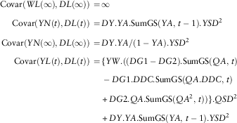 $$\eqalignno{ \cr{\rm Covar(}WL(\infty),DL(\infty){\rm )}\,=\, & \infty \cr {\rm Covar(}YN(t),DL(t){\rm )}\,=\, & DY.YA.{\rm SumGS(}YA,\,t-{\rm 1)}.YSD^{{\rm 2}} \cr {\rm Covar(}YN(\infty),DL(\infty){\rm )}\,=\, & DY.YA/({\rm 1}-YA).YSD^{{\rm 2}} \cr {\rm Covar(}YL(t),DL(t){\rm )}\,=\, & \{ YW.((DG{\rm 1}-DG{\rm 2}).{\rm SumGS(}QA,\,t{\rm )} \cr & -DG{\rm 1}.DDC.{\rm SumGS(}QA.DDC,\,t{\rm )} \cr & {\plus}DG{\rm 2}.QA.{\rm SumGS(}QA^{{\rm 2}} ,\,t{\rm )})\} .QSD^{{\rm 2}} \cr & {\plus}DY.YA.{\rm SumGS}(YA,\,t-{\rm 1}).YSD^{{\rm 2}} $$
 $$\eqalignno{ {\rm Covar(}YL(\infty),DL(\infty){\rm )}\,=\, & \{ YW.((DG{\rm 1}-DG{\rm 2})/({\rm 1}-QA) \cr & -DG{\rm 1}.DDC/({\rm 1}-QA.DDC) \cr & {\plus}DG{\rm 2}.QA/({\rm 1}-QA^{{\rm 2}} ))\} .QSD^{{\rm 2}} \cr & {\plus}DY.YA/({\rm 1}-YA).YSD^{{\rm 2}} $$
 $$\eqalignno{ {\rm Covar(}YEP(t),DL(t){\rm )}\,=\, & 0\quad \quad \quad \quad \quad \quad \quad \quad t\,=\,{\rm 1} \cr \,=\, & DY.YSD^{{\rm 2}} \quad \quad \quad \quad \,\,\,\,t\,\gt\, {\rm 1} $$
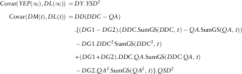 $$\eqalignno{ {\rm Covar(}YEP(\infty),DL(\infty){\rm )}\,=\, & DY.YSD^{{\rm 2}} \cr {\rm Covar(}DM(t),DL(t){\rm )}\,=\, & DD(DDC-QA) \cr & . \{ (DG{\rm 1}-DG{\rm 2}).(DDC.{\rm SumGS(}DDC,\,t{\rm )}-QA.{\rm SumGS(}QA,\,t{\rm )}) \cr & - DG{\rm 1}.DDC^{{{\rm 2}.}} {\rm SumGS(}DDC^{{\rm 2}} ,\,t{\rm )} \cr & {\plus} (DG{\rm 1}{\plus}DG{\rm 2}).DDC.QA.{\rm SumGS(}DDC.QA,\,t{\rm )} \cr & - DG{\rm 2}.QA^{{\rm 2}} .{\rm SumGS(}QA^{{\rm 2}} ,\,t{\rm )}\} .QSD^{{\rm 2}} $$
 $$\eqalignno{ {\rm Covar(}DM(\infty),DL(\infty){\rm )}\,=\, & DD(DDC-QA) \cr & . \{ (DG{\rm 1}-DG{\rm 2}).(DDC/({\rm 1}-DDC)-QA/({\rm 1}-QA)) \cr & -DG{\rm 1}.DDC^{{{\rm 2}}} /({\rm 1}-DDC^{{\rm 2}} ) \cr & {\plus}(DG{\rm 1}{\plus}DG{\rm 2}).DDC.QA/({\rm 1}-DDC.QA) \cr & -DG{\rm 2}.QA^{{\rm 2}} /({\rm 1}-QA^{{\rm 2}} )\} .QSD^{{\rm 2}} $$
 $$\eqalignno{ {\rm Covar(}DEP(t),DL(t){\rm )}\,=\, & 0\quad \quad \quad \quad \quad \quad \quad \quad \quad \quad t\,=\,{\rm 1} \cr \,=\, & ({\rm 1}{\plus}DB).DSD^{{\rm 2}} \quad \quad \quad \quad \,\,\,t\,\gt\, {\rm 1} \cr {\rm Covar(}DEP(\infty),DL(\infty){\rm )}\,=\, & ({\rm 1}{\plus}DB).DSD^{{\rm 2}} $$
 $$\vskip-10pt \eqalignno{ \cr{\rm Covar(}K(t),DL(t){\rm )}\,=\, & [(DG{\rm 1}-DG{\rm 2}).DF{\rm 1}.{\rm SumGS(}DDC,\,t{\rm )} \cr & -DG{\rm 1}.DF{\rm 1}.DDC.{\rm SumGS(}DDC^{{\rm 2}} ,\,t{\rm )} \cr & {\plus}(DG{\rm 2}.DF{\rm 1}.QA{\plus}DG{\rm 1}.DF{\rm 2}.DDC).{\rm SumGS(}DDC.QA,\,t{\rm )} \cr & -(DG{\rm 1}-DG{\rm 2}).DF{\rm 2}.{\rm SumGS(}QA,\,t{\rm )} \cr & -DG{\rm 2}.DF{\rm 2}.QA.{\rm SumGS(}QA^{{\rm 2}} ,\,t{\rm )}]\} .QSD^{{\rm 2}} \cr & {\plus}DSD^{{\rm 2}} \qquad \qquad \qquad \qquad \qquad \qquad \qquad \qquad \qquad t\,=\,{\rm 1} \cr \,=\, & [(DG{\rm 1}-DG{\rm 2}).DF{\rm 1}.{\rm SumGS(}DDC,\,t{\rm )} \cr & -DG{\rm 1}.DF{\rm 1}.DDC.{\rm SumGS(}DDC^{{\rm 2}} ,\,t{\rm )} \cr & {\plus}(DG{\rm 2}.DF{\rm 1}.QA{\plus}DG{\rm 1}.DF{\rm 2}.DDC).{\rm SumGS}\left( {DDC.QA,\,t} \right) \cr -\left( {DG{\rm 1 }-DG{\rm 2}} \right).DF{\rm 2}.{\rm SumGS}\left( {QA,\,t} \right) \cr -DG{\rm 2}.DF{\rm 2}.QA.{\rm SumGS}\left( {QA^{{\rm 2}} ,\,t} \right)]\} .QSD^{{\rm 2}} \cr \,{\plus}DY^{{\rm 2}} .YSD^{{\rm 2}} {\plus}({\rm 1}{\plus}DB.({\rm 1}{\plus}DB)).DSD^{{\rm 2}} \qquad \qquad \quad t\,\gt\, {\rm 1} $$
 $$\eqalignno{ {\rm Covar(}K(\infty),DL(\infty){\rm )}\,=\, & [(DG{\rm 1}-DG{\rm 2}).DF{\rm 1}/({\rm 1}-DDC) \cr & -DG{\rm 1}.DF{\rm 1}.DDC/({\rm 1}-{\rm }DDC^{{\rm 2}} ) \cr & {\plus}(DG{\rm 2}.DF{\rm 1}.QA{\plus}DG{\rm 1}.DF{\rm 2}.DDC)/({\rm 1}-DDC.QA) \cr & -(DG{\rm 1}-DG{\rm 2}).DF{\rm 2}/({\rm 1}-QA) \cr & -DG{\rm 2}.DF{\rm 2}.QA/({\rm 1}-QA^{{\rm 2}} )]\} .QSD^{{\rm 2}} \cr & {\plus}DY^{{\rm 2}} .YSD^{{\rm 2}} {\plus}({\rm 1}{\plus}DB.({\rm 1}{\plus}DB)).DSD^{{\rm 2}} $$
 $$\eqalignno{ {\rm Covar(}IN(t),PL(t){\rm )}\,=\, & {\rm Covar(}IN(t),DL(t){\rm )}-{\rm Covar(}IN(t),YL(t){\rm )} \cr \,=\, & [(DG{\rm 1}-DG{\rm 2}).{\rm SumGS(}QA,\,t{\rm )}-DG{\rm 1}.DDC.{\rm SumGS(}DDC.QA,\,t{\rm )} \cr & {\plus}DG{\rm 2}.QA{\rm SumGS(}QA^{{\rm 2}} ,\,t{\rm )}].QSD^{{\rm 2}} \cr & -YW.QA.{\rm SumGS(}QA^{{\rm 2}} ,\,t{\rm )}.QSD^{{\rm 2}} $$
 $$\eqalignno{ {\rm Covar(}IN(\infty),PL(\infty){\rm )}\,=\, & [(DG{\rm 1}-DG{\rm 2})/({\rm 1}-QA)-DG{\rm 1}.DDC/({\rm 1}-DDC.QA) \cr & {\plus}DG{\rm 2}.QA/({\rm 1}-QA^{{\rm 2}} )].QSD^{{\rm 2}} \cr & -YW/({\rm 1}-QA^{{\rm 2}} ).QSD^{{\rm 2}} $$
 $$\eqalignno{ {\rm Covar(}IP(t),PL(t){\rm )}\,=\, & 0\quad \quad \quad \quad \quad \quad \quad \quad \quad \quad \quad \quad \quad \quad \quad \quad \quad \quad \quad \quad \quad \quad \quad\quad \quad t\,=\,{\rm 1} \cr \,=\, & [(DG{\rm 1}-DG{\rm 2}).{\rm SumGS(}QA,\,t-{\rm 1)}-DG{\rm 1}.DDC^{{\rm 2}} .{\rm SumGS(}QA.DDC,\,t-{\rm 1)} \cr & {\plus}DG{\rm 2}.QA^{{\rm 2}} .{\rm SumGS(}QA^{{\rm 2}} ,\,t-{\rm 1)}].QSD^{{\rm 2}} \cr & -YW.QA.{\rm SumGS(}QA^{{\rm 2}} ,\,t-{\rm 1)}.QSD^{{\rm 2}} \quad \quad \quad \quad \quad \quad \quad \quad \quad t\,\gt\, {\rm 1} $$
 $$\eqalignno{ {\rm Covar(}IP(\infty),PL(\infty){\rm )}\,=\, & [(DG{\rm 1}-DG{\rm 2})/({\rm 1}-QA)-DG{\rm 1}.DDC^{{\rm 2}} /({\rm 1}-QA.DDC) \cr & {\plus}DG{\rm 2}.QA^{{\rm 2}} /({\rm 1}-QA^{{\rm 2}} ).QSD^{{\rm 2}} \cr & -YW.QA/({\rm 1}-QA^{{\rm 2}} ).QSD^{{\rm 2}} $$
 $$\eqalignno{ {\rm Covar}(QL(t),PL(t))\,=\, & {\rm Covar}(QL(t),DL(t))-{\rm Covar(}QL(t),YL(t){\rm )} \cr \,=\, & \{ DG{\rm 1}.(t-QA.{\rm SumGS(}QA,\,t{\rm )}-DDC.{\rm SumGS(}DDC,\,t{\rm )} \cr & {\plus}QA.DDC.{\rm SumGS(}QA.DDC,\,t{\rm )}) \cr & -DG{\rm 2}.(t-{\rm 2}QA.{\rm SumGS(}QA,\,t{\rm )}{\plus}QA^{{\rm 2}} .{\rm SumGS(}QA^{{\rm 2}} ,\,t{\rm )})\} \cr & /({\rm 1}-QA).QSD^{{\rm 2}} \cr & -YW/({\rm 1}-QA)\,\{ {\rm SumGS(}QA,\,t{\rm )}-QA.{\rm SumGS(}QA^{{\rm 2}} ,\,t{\rm )}\} .QSD^{{\rm 2}} $$
 $$\eqalignno{ {\rm Covar(}QL(\infty),PL(\infty){\rm )}\,=\, & \infty \cr {\rm Covar(}J(t),PL(t){\rm )}\,=\, & WW{\rm 1}.(DW.DD{\plus}DX).QSD^{{\rm 2}} -WW{\rm 1}.\,YW.\,QSD^{{\rm 2}} \quad \quad \quad \quad t\,=\,{\rm 1} \cr \,=\, & [WW{\rm 1}.(DW.DD{\plus}DX) \cr & {\plus} WQ.\{ (DG{\rm 1}-DG{\rm 2}).{\rm SumGS(}QA,\,t-{\rm 1)} \cr & -DG{\rm 1}.DDC^{{\rm 2}} .{\rm SumGS(}QA.DDC,\,t-{\rm 1)} \cr & {\plus}DG{\rm 2}.QA^{{\rm 2}} .{\rm SumGS(}QA^{{\rm 2}} ,\,t-{\rm 1)}\} ].QSD^{{\rm 2}} \cr & YW.\{ WW{\rm 1}{\plus}WQ.QA.{\rm SumGS(}QA^{{\rm 2}} ,\,t-{\rm 1)}\} .QSD^{{\rm 2}} \quad \quad \quad t\,\gt\, {\rm 1} $$
 $$\eqalignno{ {\rm Covar(}J(\infty),PL(\infty){\rm )}\,=\, & [WW{\rm 1}.(DW.DD{\plus}DX) \cr & {\plus} WQ.\{ (DG{\rm 1}-DG{\rm 2})/({\rm 1}-QA)-DG{\rm 1}.DDC^{{\rm 2}} /({\rm 1}-QA.DDC)) \cr & {\plus}DG{\rm 2}.QA^{{\rm 2}} /({\rm 1}-QA^{{\rm 2}} )\} ].QSD^{{\rm 2}} \cr & YW.\{ WW{\rm 1}{\plus}WQ.QA/({\rm 1}-QA^{{\rm 2}} )\} .QSD^{{\rm 2}} $$
 $$\eqalignno{ {\rm Covar(}WL(t),PL(t){\rm )}\,=\, & WW{\rm 1}.(DW.DD{\plus}DX).QSD^{{\rm 2}} -WW{\rm 1}.YW.QSD^{{\rm 2}} \quad \quad \quad \quad \quad \quad \quad t\,=\,{\rm 1} \cr \,=\, & [WW{\rm 1}.(DW.DD{\plus}DX) \cr & {\plus}\{ WW{\rm 1}.[(DG{\rm 1}-DG{\rm 2}).(t-{\rm 1})-DG{\rm 1}.DDC^{{\rm 2}} .{\rm SumGS(}DDC,\,t-{\rm 1)} \cr & {\plus}DG{\rm 2}.QA^{{\rm 2}} .{\rm SumGS(}QA,\,t-{\rm 1)}] \cr & {\plus}WQ/({\rm 1}-QA).[(DG{\rm 1}-DG{\rm 2}).(t-{\rm 1})-QA.{\rm SumGS(}QA,\,t-{\rm 1)}) \cr & -DG{\rm 1}.DDC^{{\rm 2}} ({\rm SumGS(}DDC,\,t-{\rm 1)}-QA.{\rm SumGS(}QA.DDC,\,t-{\rm 1)}) \cr & {\plus}DG{\rm 2}.QA^{{\rm 2}} .({\rm SumGS(}QA,\,t-{\rm 1)}-QA.{\rm SumGS(}QA^{{\rm 2}} ,\,t-{\rm 1)})\} ].QSD^{{\rm 2}} \cr & -YW.\{ WW{\rm 1}{\plus}(WW{\rm 1}{\plus}WQ/({\rm 1}-QA)).QA.{\rm SumGS(}QA,\,t-{\rm 1)} \cr & -WQ/({\rm 1}-QA).QA^{{\rm 2}} .{\rm SumGS}(QA^{{\rm 2}} ,\,t-{\rm 1}\} .QSD^{{\rm 2}} \quad \quad \quad \quad \quad t\,\gt\, {\rm 1} $$
 $$\eqalignno{ {\rm Covar(}WL(\infty),PL(\infty){\rm )}\,=\, & \infty \cr {\rm Covar(}YN(t),PL(t){\rm )}\,=\, & DY.YA.{\rm SumGS(}YA,\,t-{\rm 1)}.YSD^{{\rm 2}} -{\rm SumGS(}YA^{{\rm 2}} ,\,t{\rm )}.YSD^{{\rm 2}} \cr {\rm Covar(}YN(\infty),PL(\infty){\rm )}\,=\, & DY.YA/({\rm 1}-YA).YSD{\rm 2}-{\rm 1}/({\rm 1}-YA^{{\rm 2}} ).YSD^{{\rm 2}} \cr {\rm Covar(}YL(t),PL(t){\rm )}\,=\, & {\rm Covar(}YL{\rm (}t{\rm )},DL{\rm (}t{\rm ))}-{\rm Var[}YL{\rm (}t{\rm )]} \cr \,=\, & \{ YW.((DG{\rm 1}-DG{\rm 2}).{\rm SumGS(}QA,\,t{\rm )} \cr &-DG{\rm 1}.DDC.{\rm SumGS(}QA.DDC,\,t{\rm )} \cr & {\plus}DG{\rm 2}.QA.{\rm SumGS(}QA^{{\rm 2}} ,\,t{\rm )})\} .QSD^{{\rm 2}} \cr & {\plus}DY.YA.{\rm SumGS(}YA,\,t-{\rm 1)}.YSD^{{\rm 2}} \cr & -YW^{{\rm 2}} .{\rm SumGS(}QA^{{\rm 2}} ,\,t{\rm )}).QSD^{{\rm 2}} -{\rm SumGS(}YA^{{\rm 2}} ,\,t{\rm )}.YSD^{{\rm 2}} $$
 $$\eqalignno{ {\rm Covar(}YL(\infty),PL(\infty){\rm )}\,=\, & \{ YW.((DG{\rm 1}-DG{\rm 2})/({\rm 1}-QA) \cr & -DG{\rm 1}.DDC/({\rm 1}-QA.DDC) \cr &{\plus}DG{\rm 2}.QA/({\rm 1}-QA^{{\rm 2}} ))\} .QSD^{{\rm 2}} \cr & {\plus}DY.YA/({\rm 1}-YA).YSD^{{\rm 2}} \cr & -YW^{{\rm 2}} /({\rm 1}-QA^{{\rm 2}} ).QSD^{{\rm 2}} -{\rm 1}/{\rm (1}-YA^{{\rm 2}} {\rm )}.YSD^{{\rm 2}} $$
 $$\eqalignno{ {\rm Covar(}YEP(t),PL(t){\rm )}\,=\, & 0\quad \quad \quad \quad \quad \quad \quad \quad \quad \quad \,\,\,t\,=\,{\rm 1} \cr \,=\, & DY.YSD^{{\rm 2}} -YA.YSD^{{\rm 2}} \quad \quad \quad t\,=\,{\rm 2} \cr \,=\, & DY.YSD^{{\rm 2}} \quad \quad \quad \quad \quad \quad \quad t\,\gt\, {\rm 2} $$
 $$\eqalignno{ {\rm Covar(}YEP(\infty),PL(\infty){\rm )}\,=\, & DY.YSD^{{\rm 2}} \cr {\rm Covar(}DM(t),PL(t){\rm )}\,=\, & DD(DDC-QA) \cr & .\{ (DG{\rm 1}-DG{\rm 2}).(DDC.{\rm SumGS(}DDC,\,t{\rm )}-QA.{\rm SumGS(}QA,\,t{\rm )}) \cr & -DG{\rm 1}.DDC^{{\rm 2}} {\rm .SumGS(}DDC^{{\rm 2}} ,\,t{\rm )} \cr & {\plus}(DG{\rm 1}{\plus}DG{\rm 2}).DDC.QA.{\rm SumGS(}DDC.QA,\,t{\rm )} \cr & -DG{\rm 2}.QA^{{\rm 2}} .{\rm SumGS(}QA^{{\rm 2}} ,\,t{\rm )}\} .QSD^{{\rm 2}} \cr & -YW.DD/(DDC-QA) \cr & .\{ DDC.{\rm SumGS(}DDC.QA,\,t{\rm )}-QA.{\rm SumGS(}QA^{{\rm 2}} ,\,t{\rm )}\} .QSD^{{\rm 2}} $$
 $$\eqalignno{ {\rm Covar(}DM(\infty),PL(\infty){\rm )}\,=\, & DD(DDC-QA) \cr & .\{ (DG{\rm 1}-DG{\rm 2}).(DDC/({\rm 1}-DDC)-QA/({\rm 1}-QA)) \cr & -DG{\rm 1}.DDC^{{{\rm 2}.}} /({\rm 1}-DDC^{{\rm 2}} ) \cr & {\plus}(DG{\rm 1}{\plus}DG{\rm 2}).DDC.QA/({\rm 1}-DDC.QA) \vskip-20pt \eqalign{\cr & -DG{\rm 2}.QA^{{\rm 2}} /({\rm 1}-QA^{{\rm 2}} )\} .QSD^{{\rm 2}} \cr & -YW.DD/(DDC-QA) \cr & \ .\{ DDC/({\rm 1}-DDC.QA)-QA/({\rm 1}-QA^{{\rm 2}} )\} .QSD^{{\rm 2}} $$
$$\eqalignno{ {\rm Covar(}DEP(t),PL(t){\rm )}\,=\, & 0\quad \quad \quad \qquad \qquad \qquad \qquad \qquad \qquad \qquad \quad \quad \quad \quad \quad \quad t\,=\,{\rm 1} \cr \,=\, & ({\rm 1}{\plus}DB).DSD^{{\rm 2}} \quad \quad \quad \quad \qquad \qquad \qquad \qquad \qquad \qquad \quad \,t\,\gt\, {\rm 1} \cr {\rm Covar(}DEP(\infty),PL(\infty){\rm )}\,=\, & ({\rm 1}{\plus}DB).DSD^{{\rm 2}} \cr {\rm Covar(}K(t),PL(t){\rm )}\,=\, & [(DG{\rm 1}-DG{\rm 2}).DF{\rm 1}.{\rm SumGS(}DDC,\,t{\rm )} \cr & -DG{\rm 1}.DF{\rm 1}.DDC.{\rm SumGS(}DDC^{{\rm 2}} ,\,t{\rm )} \cr &{\plus}(DG{\rm 2}.DF{\rm 1}.QA {\plus}DG{\rm 1}.DF{\rm 2}.DDC).{\rm SumGS(}DDC.QA,\,t{\rm )} \cr & -(DG{\rm 1}-DG{\rm 2}).DF{\rm 2}.{\rm SumGS(}QA,\,t{\rm )} \cr & -DG{\rm 2}.DF{\rm 2}.QA.{\rm SumGS(}QA^{{\rm 2}} ,\,t{\rm )}]\} .QSD^{{\rm 2}} \cr & -\{ YW.[DF{\rm 1}.{\rm SumGS(}DDC.QA,\,t{\rm )}-DF{\rm 2}.{\rm SumGS(}QA^{{\rm 2}} ,\,t{\rm )}]\} .QSD^{{\rm 2}} \cr & {\plus}DSD^{{\rm 2}} \qquad \qquad \qquad \qquad \qquad \quad \quad \quad \quad \quad \quad \quad \quad \quad \quad t\,=\,{\rm 1} \cr \,=\, & [(DG{\rm 1}-DG{\rm 2}).DF{\rm 1}.{\rm SumGS(}DDC,\,t{\rm )} \cr & -DG{\rm 1}.DF{\rm 1}.DDC.{\rm SumGS(}DDC^{{\rm 2}} ,\,t{\rm )} \cr & {\plus}(DG{\rm 2}.DF{\rm 1}.QA{\plus}DG{\rm 1}.DF{\rm 2}.DDC).{\rm SumGS(}DDC.QA,\,t{\rm )} \cr & -(DG{\rm 1}-DG{\rm 2}).DF{\rm 2}.{\rm SumGS(}QA,\,t{\rm )} \cr & -DG{\rm 2}.DF{\rm 2}.QA.{\rm SumGS}\left( {QA^{{\rm 2}} ,\,t} \right)]\} .QSD^{{\rm 2}} \cr & {\plus}DY^{{\rm 2}} .YSD^{{\rm 2}} {\plus}({\rm 1}{\plus}DB.({\rm 1}{\plus}DB)).DSD^{{\rm 2}} \cr & -\{ YW.[DF{\rm 1}.{\rm SumGS(}DDC.QA,\,t{\rm )}-DF{\rm 2}.{\rm SumGS(}QA^{{\rm 2}} ,\,t{\rm )}]\} .QSD^{{\rm 2}} \cr & -YA.DY.YSD^{{\rm 2}} \quad \quad \quad \quad \quad \quad \quad \quad \quad \quad \quad \quad \quad \quad \quad \quad \quad \quad \quad \quad t\,\gt\, {\rm 1} $$
 $$\eqalignno{ {\rm Covar(}K(\infty),PL(\infty){\rm )}\,=\, & [(DG{\rm 1}-DG{\rm 2}).DF{\rm 1}/({\rm 1}-DDC) \cr & -DG{\rm 1}.DF{\rm 1}.DDC/({\rm 1}-DDC^{{\rm 2}} ) \cr & {\plus}(DG{\rm 2}.DF{\rm 1}.QA{\plus}DG{\rm 1}.DF{\rm 2}.DDC)/({\rm 1}-DDC.QA) \cr & -(DG{\rm 1}-DG{\rm 2}).DF{\rm 2}/({\rm 1}-QA) \cr & -DG{\rm 2}.DF{\rm 2}.QA/({\rm 1}-QA^{{\rm 2}} )]\} .QSD^{{\rm 2}} \cr & {\plus}DY^{{\rm 2}} .YSD^{{\rm 2}} {\plus}({\rm 1}{\plus}DB.({\rm 1}{\plus}DB)).DSD^{{\rm 2}} \cr & -\{ YW.[DF{\rm 1}/({\rm 1}-DDC.QA)-DF{\rm 2}/({\rm 1}-QA^{{\rm 2}} )]\} .QSD^{{\rm 2}} \cr & -YA.DY.YSD^{{\rm 2}} $$
$$\openup 2pt\eqalignno{ {\rm Covar(}DL(t),PL(t){\rm )}\,=\, & {\rm Var[}DL{\rm (}t{\rm )]}-{\rm Covar}\left( {YL\left( t \right),DL\left( t \right)} \right) \cr \,=\, & {\rm }\left( {DF{\rm 1}-DF{\rm 2}} \right)^{{\rm 2}} .QSD^{{\rm 2}} {\plus}DSD^{{\rm 2}} \cr & -\{ YW.((DG{\rm 1}-DG{\rm 2}).{\rm SumGS(}QA,\,t{\rm )} \cr & -DG{\rm 1}.DDC.{\rm SumGS(}QA.DDC,\,t{\rm )} \cr &{\plus}DG{\rm 2}.QA.{\rm SumGS(}QA^{{\rm 2}} ,\,t{\rm )})\} .QSD^{{\rm 2}} \cr & -DY.YA.{\rm SumGS}\left( {YA,\,t-{\rm 1}} \right).YSD^{{\rm 2}} \quad \qquad \qquad \qquad \quad \quad \quad t\,=\,{\rm 1} \cr \,=\, & \{ (DG{\rm 1}-DG{\rm 2})^{{\rm 2}} .t-{\rm 2}DG{\rm 1}.(DG{\rm 1}-DG{\rm 2})DDC.{\rm SumGS(}DDC,\,t{\rm )} \cr & {\plus}DG{\rm 1}^{{\rm 2}} DDC^{{\rm 2}} .{\rm SumGS(}DDC^{{\rm 2}} ,\,t{\rm )} \cr & -{\rm 2}.DG{\rm 1}.DG{\rm 2}.QA.DDC.{\rm SumGS(}QA.DDC,\,t{\rm )} \cr & {\plus}{\rm 2}DG{\rm 2}.\left( {DG{\rm 1}-DG{\rm 2}} \right).QA.{\rm SumGS}\left( {QA,\,t} \right) \cr & {\plus}DG{\rm 2}^{{\rm 2}} .QA^{{\rm 2}} {\rm SumGS(}QA^{{\rm 2}} ,\,t{\rm )}\} .QSD^{{\rm 2}} \cr & {\plus}(t-{\rm 1}).DY^{{\rm 2}} YSD^{{\rm 2}} {\plus}\{ {\rm 1}{\plus}(t-{\rm 1}).({\rm 1}{\plus}DB)^{{\rm 2}} \} .DSD^{{\rm 2}} \cr & -\{ YW.((DG{\rm 1}-DG{\rm 2}).{\rm SumGS(}QA,\,t{\rm )} \cr & -DG{\rm 1}.DDC.{\rm SumGS(}QA.DDC,\,t{\rm )} \cr & {\plus}DG{\rm 2}.QA.{\rm SumGS(}QA^{{\rm 2}} ,\,t{\rm )})\} .QSD^{{\rm 2}} \cr & -DY.YA.{\rm SumGS(}YA,\,t-{\rm 1)}.YSD^{{\rm 2}} \quad \quad \qquad \qquad \qquad \qquad \quad t\,\gt\, {\rm 1} $$
 $${\rm Covar(}DL(\infty),PL(\infty){\rm )}\,=\,\infty$$
A.5.6. Long-term interest rates
 $$\eqalignno{ {\rm Covar(}IN(t),CM(t){\rm )}\,=\, & CD/(CDC-QA) \cr & .\{ CDC.{\rm SumGS(}QA.CDC,\,t{\rm )}-QA.{\rm SumGS(}QA^{{\rm 2}} ,\,t{\rm )}\} .QSD^{{\rm 2}} \cr {\rm Covar(}IN(\infty),CM(\infty){\rm )}\,=\, & CD/(CDC-QA) \cr & .(CDC/({\rm 1}-QA.CDC)-QA/({\rm 1}-QA^{{\rm 2}} ))\} .QSD^{{\rm 2}} \cr {\rm Covar(}IP(t),CM(t){\rm )}\,=\, & 0\quad \quad \quad \quad \quad \quad \quad \quad \quad \quad \quad \quad \quad \quad \quad \quad \quad \quad \qquad \qquad \qquad \quad t\,=\,{\rm 1} \cr \,=\, & CD/(CDC-QA)\,\{ CDC^{{\rm 2}} .{\rm SumGS(}QA.CDC,\,t-{\rm 1)} \cr & -QA^{{\rm 2}} .{\rm SumGS(}QA^{{\rm 2}} ,\,t-{\rm 1)})\} .QSD^{{\rm 2}} \quad \qquad \qquad \qquad \quad \quad \quad t\,\gt\, {\rm 1} $$
 $$\vskip-12pt \eqalignno{ {\rm Covar(}IP(\infty),CM(\infty){\rm )}\,=\, & CD/(CDC-QA) \cr & .({\rm 1}/({\rm 1}-QA.CDC)-QA^{{\rm 2}} /({\rm 1}-QA^{{\rm 2}} ))\} .QSD^{{\rm 2}} \cr {\rm Covar(}QL\left( t \right),CM\left( t \right){\rm )}\,=\, & CD/\{ ({\rm 1}-QA).(CDC-QA)\} \cr & .(CDC.{\rm SumGS(}CDC,\,t{\rm )}-QA.{\rm SumGS(}QA,\,t{\rm )} \cr & -QA.CDC.{\rm SumGS(}QA.CDC,\,t{\rm )}{\plus}QA^{{\rm 2}} .{\rm SumGS(}QA^{{\rm 2}} ,\,t{\rm )}).QSD^{{\rm 2}} \vskip-35pt \eqalign{\cr {\rm Covar(}QL(\infty),CM(\infty){\rm )}\,=\, & CD/\{ ({\rm 1}-QA).(CDC-QA)\} \cr & .\{ CDC/({\rm 1}-CDC)-QA/({\rm 1}-QA)-QA.CDC/({\rm 1}-QA.CDC) \cr & {\plus}QA^{{\rm 2}} /({\rm 1}-QA^{{\rm 2}} )\} .QSD^{{\rm 2}} $$
 $$\eqalignno{ {\rm Covar(}J(t),CM(t){\rm )}\,=\, & WW{\rm 1}.CD.QSD^{{\rm 2}} \quad \quad \quad \quad \quad \quad \quad \quad \quad \quad \quad \quad \quad \quad \quad t\,=\,{\rm 1} \cr \,=\, & [WW{\rm 1}.CD{\plus}WQ.CD/(CDC-QA) \cr & .\{ CDC^{{\rm 2}} .{\rm SumGS(}QA.CDC,\,t-{\rm 1)} \cr & -QA^{{\rm 2}} .{\rm SumGS(}QA^{{\rm 2}} ,\,t-{\rm 1)}\} ].QSD^{{\rm 2}} \qquad \qquad \quad \quad \quad t\,\gt\, {\rm 1} \cr {\rm Covar(}J(\infty),CM(\infty){\rm )}\,=\, & [WW{\rm 1}.CD{\plus}WQ.CD/(CDC-QA). \cr & \{ CDC^{{\rm 2}} /({\rm 1}-QA.CDC)-QA^{{\rm 2}} /({\rm 1}-QA^{{\rm 2}} )\} ].QSD^{{\rm 2}} \cr {\rm Covar(}WL(t),CM(t){\rm )}\,=\, & WW{\rm 1}.CD.QSD^{{\rm 2}} \quad \quad \quad \quad \quad \quad \quad \quad \quad \quad \quad \quad \quad \quad \quad t\,=\,{\rm 1} \cr \,=\, & [WW{\rm 1}.CD{\plus}CD/(CDC-QA) \cr & .\{ (WW{\rm 1}{\plus}WQ/({\rm 1}-QA)).(CDC^{{\rm 2}} .{\rm SumGS(}CDC,\,t-{\rm 1)} \cr & -QA^{{\rm 2}} {\rm SumGS(}QA,\,t-{\rm 1)}) \cr & -WQ/({\rm 1}-QA).QA.(CDC^{{\rm 2}} .{\rm SumGS(}QA.CDC,\,t-{\rm 1)} \cr & {\plus}QA^{{\rm 2}} .{\rm SumGS(}QA^{{\rm 2}} ,\,t-{\rm 1)}\} ].QSD^{{\rm 2}} \quad \quad \qquad \qquad \quad \quad t\,\gt\, {\rm 1} $$
 $$\eqalignno{ {\rm Covar(}WL(\infty),CM(\infty){\rm )}\,=\, & [WW{\rm 1}.CD{\plus}CD/(CDC-QA) \cr & \{ (WW{\rm 1}{\plus}WQ/({\rm 1}-QA).[CDC^{{\rm 2}} /({\rm 1}-CDC)-QA^{{\rm 2}} /({\rm 1}-QA)] \cr & -WQ/({\rm 1}-QA).QA.[CDC^{{\rm 2}} /({\rm 1}-CDC)-QA^{{\rm 2}} /({\rm 1}-QA)\} ].QSD^{{\rm 2}} $$
 $$\eqalignno{ {\rm Covar(}YL(t),CM(t){\rm )}\,=\, & YW.CD/(CDC-QA). \cr & .\{ CDC.{\rm SumGS(}CDC.QA,\,t{\rm )}-QA.{\rm SumGS(}QA^{{\rm 2}} ,\,t{\rm )}\} .QSD^{{\rm 2}} $$
 $$\eqalignno{ {\rm Covar}\left( {YL(\infty),CM(\infty)} \right)\,=\, & YW.CD/(CDC-QA) \cr & .\{ CDC/({\rm 1 }-CDC.QA)-QA/({\rm 1 }-QA^{{\rm 2}} )\} .QSD^{{\rm 2}} $$
 $$\eqalignno{ {\rm Covar(}DM(t),CM(t){\rm )}\,=\, & DD.CD/\{ (DDC-QA).(CDC-QA)\} \cr & .\{ DDC.CDC.{\rm Sum(}DDC.CDC,\,t{\rm )}-DDC.QA.{\rm Sum(}DDC.QA,\,t{\rm )} \cr & -QA.CDC.{\rm Sum(}QA.CDC,\,t{\rm )}{\plus}QA^{{\rm 2}} {\rm Sum(}QA^{{\rm 2}} ,\,t{\rm )}.QSD^{{\rm 2}} $$
 $$\eqalignno{ {\rm Covar(}DM(\infty),CM(\infty){\rm )}\,=\, & DD.CD/\left\{ {(DDC-QA).(CDC-QA)} \right\} \cr & .\{ DDC.CDC/({\rm 1}-DDC.CDC)-DDC.QA/({\rm 1}-DDC.QA) \cr & -QA.CDC/({\rm 1}-QA.CDC){\plus}QA^{{\rm 2}} /({\rm 1}-QA^{{\rm 2}} ).QSD^{{\rm 2}} $$
 $$\eqalignno{ {\rm Covar(}K(t),CM(t){\rm )}\,=\,&\{ CD/(CDC- QA).[DF{\rm 1}.CDC.{\rm SumGS(}DDC.CDC,\,t{\rm )} \cr & -DF{\rm 1}.QA.{\rm SumGS(}DDC.QA,\,t{\rm )} \cr & -DF{\rm 2}.CDC.{\rm SumGS(}QA.CDC,\,t{\rm )} \cr & {\plus}DF{\rm 2}.QA.{\rm SumGS(}QA^{{\rm 2}} ,\,t{\rm )})].QSD^{{\rm 2}} $$
 $$\eqalignno{ {\rm Covar(}K(\infty),CM(\infty){\rm )}\,=& \,\{ CD/( CDC-QA).[DF{\rm 1}.CDC/({\rm 1}-DDC.CDC) \cr & -DF{\rm 1}.QA/({\rm 1}-DDC.QA)-DF{\rm 2}.CDC/({\rm 1}-QA.CDC) \cr & {\plus}DF{\rm 2}.QA/({\rm 1}-QA^{{\rm 2}} ))].QSD^{{\rm 2}} $$
 $$\eqalignno{ {\rm Covar(}DL(t),CM(t){\rm )}\,=\, & CD/(CDC-QA) \cr & .(DG{\rm 1}-DG{\rm 2}).(CDC.{\rm SumGS(}CDC,\,t{\rm )}-QA.{\rm SumGS(}QA,\,t{\rm )}) \cr & -DG{\rm 1}.DDC.(CDC.{\rm SumGS(}DDC.CDC,\,t{\rm )}-QA.{\rm SumGS(}DDC.QA,\,t{\rm )}) \cr & {\plus}DG{\rm 2}.QA.(CDC.{\rm SumGS(}QA.CDC,\,t{\rm )}-QA.{\rm SumGS(}QA^{{\rm 2}} ,\,t{\rm )}).QSD^{{\rm 2}} $$
 $$\eqalignno{ {\rm Covar(}DL(\infty) ,CM(\infty){\rm )}\,=\,& CD/(CDC-QA) \cr & .(DG{\rm 1}-DG{\rm 2}).(CDC/({\rm 1}-CDC)-QA/({\rm 1}-QA)) \cr & -DG{\rm 1}.DDC.(CDC/({\rm 1}-DDC.CDC)-QA/({\rm 1}-DDC.QA)) \cr & {\plus}DG{\rm 2}.QA.(CDC/({\rm 1}-QA.CDC)-QA/({\rm 1}-QA^{{\rm 2}} )).QSD^{{\rm 2}} $$
 $$\eqalignno{ {\rm Covar(}PL(t),CM(t){\rm )}\,=\, & {\rm Covar(}DL(t),CM(t){\rm )}-{\rm Covar(}YL(t),CM(t){\rm )} \cr \,=& \,CD/(CDC-QA) \cr &\ .(DG{\rm 1}-DG{\rm 2}).(CDC.{\rm SumGS(}CDC,\,t{\rm )}-QA.{\rm SumGS(}QA,\,t{\rm )}) \cr & -DG{\rm 1}.DDC.(CDC.{\rm SumGS(}DDC.CDC,\,t{\rm )}-QA.{\rm SumGS(}DDC.QA,\,t{\rm )}) \vskip-23pt \eqalign{\cr & {\plus}DG{\rm 2}.QA.(CDC.{\rm SumGS(}QA.CDC,\,t{\rm )}-QA.{\rm SumGS(}QA^{{\rm 2}} ,\,t{\rm )}).QSD^{{\rm 2}} \cr & -YW.CD/(CDC-QA) \cr & .\{ CDC.{\rm SumGS(}CDC.QA,\,t{\rm )}-QA.{\rm SumGS(}QA^{{\rm 2}} ,\,t{\rm )}\} .QSD^{{\rm 2}} $$
 $$\eqalignno{ {\rm Covar(}PL(\infty) ,CM(\infty){\rm )}\,=\,& CD/(CDC-QA) \cr & .(DG{\rm 1}-DG{\rm 2}).(CDC/({\rm 1}-CDC)-QA/({\rm 1}-QA)) \cr & -DG{\rm 1}.DDC.(CDC/({\rm 1}-DDC.CDC)-QA/({\rm 1}-DDC.QA)) \cr & {\plus}DG{\rm 2}.QA.(CDC/({\rm 1}-QA.CDC)-QA/({\rm 1}-QA^{{\rm 2}} )).QSD^{{\rm 2}} \cr & -YW.CD/(CDC-QA) \cr & .\{ CDC/({\rm 1}-CDC.QA)-QA/({\rm 1}-QA^{{\rm 2}} )\} .QSD^{{\rm 2}} $$
$$\eqalignno{ {\rm Covar(}YN(t),CRL(t){\rm )}\,=\, & CY.{\rm SumGS(}YA.CY,\,t{\rm )}.YSD^{{\rm 2}} \cr {\rm Covar(}YN(\infty),CRL(\infty){\rm )}\,=\, & CY/({\rm 1}-YA.CY).YSD^{{\rm 2}} \cr {\rm Covar(}YL(t),CRL(t){\rm )}\,=\, & CY.{\rm SumGS(}YA.CY,\,t{\rm )}.YSD^{{\rm 2}} \cr {\rm Covar(}YL(\infty),CRL(\infty){\rm )}\,=\, & CY/({\rm 1}-YA.CY).YSD^{{\rm 2}} \cr {\rm Covar(}YEP(t),CRL(t){\rm )}\,=\, & 0\qquad \qquad \qquad \qquad \qquad \quad \quad \quad \quad \quad \quad \quad \quad \quad \quad \quad \quad \quad \quad t\,=\,{\rm 1} \cr \,=\, & CY.CA.YSD^{{\rm 2}} \quad \quad \qquad \ \quad \qquad \qquad \qquad \quad \quad \quad \quad \quad \quad \quad \;t\,\gt\, {\rm 1} \cr {\rm Covar(}YEP(\infty),CRL(\infty){\rm )}\,=\, & CY.CA.YSD^{{\rm 2}} \cr {\rm Covar(}K(t),CRL(t){\rm )}\,=\, & 0\quad \quad \quad \quad \quad \quad \quad \quad \quad \quad \qquad \qquad \qquad \qquad \quad \quad \quad \qquad \quad t\,=\,{\rm 1} \cr \,=\, & DY.CY.CA.YSD^{{\rm 2}} \quad \qquad \qquad \qquad \quad \ \ \quad \quad \quad \quad \quad \quad \quad \quad t\,\gt\, {\rm 1} \cr {\rm Covar(}K(\infty),CRL(\infty){\rm )}\,=\, & DY.CY.CA.YSD^{{\rm 2}} \cr {\rm Covar(}DL(t),CRL(t){\rm )}\,=\, & 0\qquad \quad \quad \quad \quad \quad \quad \quad \quad \quad \quad \quad \quad \qquad \qquad \qquad \qquad \ \ \quad t\,=\,{\rm 1} \cr \,=\, & DY.CY.CA.{\rm SumGS(}CA,\,t-{\rm 1)}.YSD^{{\rm 2}} \qquad \qquad \qquad \ \ \quad \;\;t\,\gt\, {\rm 1} \cr {\rm Covar(}DL(\infty),CRL(\infty))\,=\, & DY.CY.CA/({\rm 1}-CA).YSD^{2} \cr {\rm Covar(}PL(t),CRL(t){\rm )}\,=\, & -CY.YSD^{{\rm 2}} \quad \qquad \ \ \ \ \quad \quad \quad \quad \quad \quad \quad \quad \quad \quad \quad \quad \quad \quad \;t\,=\,{\rm 1} \cr \,=\, & \{ CY.-{\rm 1}{\plus}DY.CA.{\rm SumGS(}CA,\,t-{\rm 1)} \cr & -YA.CA.{\rm SumGS(}YA.CA,\,t-{\rm 1)\} }.YSD^{{\rm 2}} \quad \qquad \qquad \quad \ \ t\,\gt\, {\rm 1} \cr {\rm Covar(}PL(\infty),CRL(\infty){\rm )}\,=\, & CY.\left\{ {-{\rm 1}{\plus}DY.CA/({\rm 1}-CA)-YA.CA/({\rm 1}-YA.CA)} \right\}.YSD^{{\rm 2}} $$
A.5.7. Short-term interest rates
BD(t) depends only on BZ(t), and no other variable is connected with it, so all covariances are zero.
A.5.8. Index-linked rates
 $$\eqalignno{ {\rm Covar[}CRL(t),R(t){\rm ]}\,=\, & RBC.{\rm SumGS}(CA.RA,\,t\} .CSD^{{\rm 2}} \cr {\rm Covar(}CRL(\infty),R(\infty){\rm )}\,=\, & RBC/({\rm 1}-CA.RA).CSD^{{\rm 2}} $$
Corrigenda
In Part 1, Table 8.1 was incorrectly presented, with three columns of numbers all the same, and all with wrong numbers in it, although the totals and the conclusions were correct.
Comparison of actual and expected values of lnR(t), 1995−2009, conditional on Ft−1 and on CE(t).
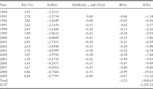
In Part 1, ¶8.8, the possible parameters were given as:
 $$RMU\,=\,{\rm 3}\,\%\,;\,RA\,=\,0.{\rm 95};\,RBC\,=\,0.00{\rm 8};\,RSD\,=\,0.{\rm 3}$$
The last should have been RSD=0.003.