INTRODUCTION
As stated by the last report on climate change effects (IPCC Reference Parry, Canziani, Palutikof, van der Linden and Hanson2007), Mediterranean regions can expect higher temperatures, less water availability and an increase in drought frequency. Irrigated agriculture could face serious risks in southern Europe in the near future, due to water scarcity and the potential increase in evapotranspiration (ET) rates (EEA 2007). This is an important problem in Spain, where irrigation uses about 0·70 of the available water (MAPA 2005).
According to Iglesias et al. (Reference Iglesias, Estrela, Gallart and Moreno2005), some Spanish regions can expect up to 50% reduction in water availability by the end of the century, although there is significant spatial variability and general uncertainty. Consequently, the Spanish government launched a strategy to address climate change issues in certain sectors (OECC 2006). The first task consisted of developing local climate change scenarios, downscaling several global circulation models (Brunet et al. Reference Brunet, Casado, De Castro, Galán, Lopez, Martín, Pastor, Petisco, Ramos, Ribalaygua, Rodríguez, Sanz and Torres2007). Evaluating future crop water requirements and comparing those demands with probable future water availability were the subsequent tasks in the Spanish strategy for climate change adaptation (OECC 2006).
Irrigation is an important component of Spanish agricultural costs, especially those related to energy. The current flooding irrigation systems are rather inefficient in Spain and other southern European countries (Neira et al. Reference Neira, Alvarez, Cuesta and Cancela2005; Playan & Mateos Reference Playan and Mateos2005). In addition, irrigation is not only expensive but can also be a potential source of water-table contaminants. However, irrigation allows farmers to obtain higher yields regularly, provides jobs and helps to keep population in rural areas (MAPA 2005). Therefore, Spain is investing more than €5 billion (mainly from public funds, with c. 0·15 of the total coming from farmers) to modernize irrigation and to reduce the water and energy losses in an environmentally sustainable way (MAPA 2005). The investment provides modern sprinkler systems and better water supplies in the most important irrigated areas. The water savings after modernization could reach c. 2×10¹⁵ m3/year (MAPA 2005).
Existing climate data (MAPA 2005) were used to design the system and for calculating the irrigation reliability of the new systems. However, current system designs might not be adequate to cope with future climate change. Policy makers and stakeholders should introduce adaptation measures in the sector, estimating the future constraints of present irrigation designs. Since farmers are paying part of the cost, they are also very interested in knowing whether the system will be reliable in the future.
Many studies on the impacts of climate change on agriculture have been published to date, with several of these having been conducted in Spain (Semenov et al. Reference Semenov, Wolf, Evans, Eckersten and Iglesias1996; Iglesias et al. Reference Iglesias, Rosenzweig and Pereira2000; Guereña et al. Reference Guereña, Ruiz-Ramos, Díaz-Ambrona, Conde and Mínguez2001; Iglesias & Quiroga Reference Iglesias and Quiroga2007; Mínguez et al. Reference Mínguez, Ruiz-Ramos, Díaz-Ambrona, Quemada and Sau2007). Nevertheless, these have been aimed mainly at estimating future crop yields rather than evaluating future water requirements and none of the studies mentioned have evaluated the performance of current irrigation systems to pridict future performance. The present paper uses a simple methodology to estimate the effects of climate change on crop water requirements. A case study is conducted, considering the main irrigated crops in the Spanish Northern Plateau. Moreover, the reliability of a recently built system, which was designed using historical data, is evaluated considering climate change scenarios.
MATERIALS AND METHODS
System design and the evaluation procedure
The capability of an irrigation system constructed in Valladolid, Northern Spain (41°39′N, 4°43′W) for coping with future water demands was evaluated. The site is at 690 m asl, with an annual average rainfall of 435 mm. An irrigation district of 610 ha received a new conduction, distribution and pumping system in the framework of the national irrigation plan with a total investment of more than €800 000 (ITACyL 2007). Water and energy costs of this new system are c. 0·31 and 0·57 of those before modernization, while irrigation application efficiency improved by 30% (ITACyL 2007). This system is representative of the irrigation modernization effort conducted in Castilla y Leon and has been used previously as a reference (ITACyL 2007; Utset Reference Utset and Utset2009).
Geographically, Castilla y León is located in northwest Spain. It is a large plateau and over 0·95 of it is more than 600 m asl. According to the Papadakis (Reference Papadakis1966) climatic classification, most of the Castilla y León area corresponds to Mediterranean Template, combining cold winters with dry hot summers: maximum and minimum average temperatures in the region are 17 and 5°C, respectively. Agriculture is constrained to the summer months, due to regular freezing between October and March. This differentiates agriculture in Castilla y Leon with other regions of southern and eastern Spain.
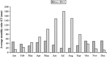
Castilla y Leon has the second-largest irrigated area in Spain, comprising more than 500 000 ha (MAPA 2005). Irrigation throughout Spain generally uses c. 0·70 of the total water. Groundwater sources represent only 0·23 of irrigation water, while reservoirs provide the rest. Flooding and sprinkler irrigations are applied to 0·61 and 0·39 of the irrigated area, respectively; however, the sprinkler proportion has increased over the last few years (MAPA 2005). The monthly averages of the recorded precipitations for the last 25 years and Penman–Monteith ET for a hypothetical grass reference crop (Allen et al. Reference Allen, Baker, Segarra and Brown2007) are shown in Fig. 1: as can be seen in the figure, rainfall is very scarce from May to October. Irrigation is required particularly for crops such as sugar beet, maize or potatoes, since summer precipitation is very scarce and ET rates are very high.
Averages of total monthly rainfall and ET in Valladolid from 1966 to 2006.

Following MAPA (2005) recommendations, the system was designed for typical demands in July, since it is the month of maximum ET. The historical averages of July meteorological data were used to compute a reference ET. The gross water requirements were estimated for a typical combination of crops in the zone, using the crop single coefficients (Kc) recommended by Allen et al. (Reference Allen, Baker, Segarra and Brown2007) and subtracting the historical effective precipitation. The effective precipitation is calculated from the Soil Conservation Service method as modified by Ferrer (Reference Ferrer1993) to Spanish conditions. The net demand was calculated according to an expected system efficiency of 0·75, as in the system design. The instantaneous maximum water supply was calculated from the net demand, assuming irrigation for 18 h, 6 days a week. According to the conducted design, the pumping system must supply at least 1 litre/s/ha in order to provide enough water to fulfil irrigation requirements in the zone (ITACyL 2007). The irrigation network was designed according to this maximum water supply.
Although Penman–Monteith calculations are used routinely for irrigation recommendations, the crop-water demands in the present paper have been calculated using the method proposed by Priestley & Taylor (Reference Priestley and Taylor1972) due to the lack of historical meteorological data. Both approaches have been found to be statistically equivalent while conducting modelling studies in Spain (Utset et al. Reference Utset, Farre, Martínez-Cob and Cavero2004). Furthermore, Priestley & Taylor's method is considered for calculating water demands in models such as DSSAT and CROPSYST (Jones et al. Reference Jones, Hoogenboom, Porter, Boote, Batchelor, Hunt, Wilkens, Singh, Gijsman and Ritchie2003; Stockle et al. Reference Stockle, Donatelli and Nelson2003), which are the crop models most used in climate change impact assessments in agriculture (Alexandrov Reference Alexandrov, Dunkel, Alexandrov, Gat, Guerreiro, Kleschenko and Ozalp2002; Tubiello & Ewert Reference Tubiello and Ewert2002).
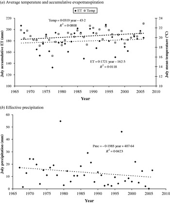
According to Priestley & Taylor's method, the average July ET from 1966 to 2006 was 181 mm, with a s.d. of 18 mm. Figure 2a depicts the changes in July ET and temperatures since 1966, while Fig. 2b shows the effective July precipitations during the same period. Figure 2 reveals no statistically significant changes but trends of increasing temperatures and decreasing precipitation, which agrees with several climate change assessments (Moreno Reference Moreno2005; Iglesias & Quiroga Reference Iglesias and Quiroga2007; IPCC Reference Parry, Canziani, Palutikof, van der Linden and Hanson2007). ET also shows a non-significant positive trend. Priestley & Taylor's calculations are highly dependent on temperature, and so the agreement between trends could be expected. However, ET values are more variable because they depend not only on temperatures but also on solar radiation. The differences between later ET values and mean ET are lower than the s.d. Nevertheless, the trend indicates that the use of historical ET averages would not be representative of future conditions, particularly if July temperatures increase by several °C, as predicted from climate change assessments. Moreover, the decline in July effective precipitation also suggests that considering the historical average could result in overestimation of future rainfall supply. However, Brunet et al. (Reference Brunet, Casado, De Castro, Galán, Lopez, Martín, Pastor, Petisco, Ramos, Ribalaygua, Rodríguez, Sanz and Torres2007) showed that uncertainty of precipitation behaviour for northern Spain during the 20th century is very large, much higher than for the expected temperature rise.
Trends in July average temperatures and accumulated ET and effective precipitation from 1966 to 2006. Regression lines and equations are shown.

The approach of MAPA (2005) was followed in the present study, assuming that 610 ha were planted with maize (0·40 of the area), sugar beet (0·35) and potato (0·25). According to Utset et al. (Reference Utset, Del Río, Martínez, Martínez, Provedo and Martín2006), this is a typical crop distribution in the region. The Kc coefficients currently used for irrigation recommendations in Castilla y Leon for July were considered (www.inforiego.org, verified 3 November 2010), which is derived from Penman–Monteith ET calculations. These were linearly transformed to Priestley & Taylor values using the relationship explained in Utset et al. (Reference Utset, Farre, Martínez-Cob and Cavero2004). The mean average demand of a single hectare depends on the above crop distribution and Kc, as well as on the July maximum ET rates.
Climate change scenarios
As a part of the Spanish Strategy for Climate Change Adaptation (OECC 2006), downscaled scenarios for the whole country have been developed. The present work considered the global circulation model (GCM) outputs from the ECHAM4 and the coupled general circulation (CGM)2 for the A2 and B2 emission scenarios, downscaled to the Valladolid meteorological station by statistical methods. The technical details of the downscaling methods can be found in Brunet et al. (Reference Brunet, Casado, De Castro, Galán, Lopez, Martín, Pastor, Petisco, Ramos, Ribalaygua, Rodríguez, Sanz and Torres2007), who used the analogue method (Wilby & Wigley Reference Wilby, Wigley and Sivakumar2000) to statistically downscale the ECHAM4 and the CGM2 GCM outputs for the A2 and B2 emission scenarios to all the Spanish meteorological stations. The analogue method has been successfully used by Wetterhall et al. (Reference Wetterhall, Halldin and Xu2005), Timbal & Jones (Reference Timbal and Jones2006) and Timbal et al. (Reference Timbal, Fernandez and Li2009) to downscale GCM outputs.
The information required to calculate Priestley & Taylor ET values comprises maximum and minimum temperatures and solar radiation. Therefore, the daily values of maximum and minimum temperatures of each of those GCM and SRES scenarios for the 2011–40, 2041–70 and 2071–2100 periods, as downscaled to the Valladolid station (Brunet et al. Reference Brunet, Casado, De Castro, Galán, Lopez, Martín, Pastor, Petisco, Ramos, Ribalaygua, Rodríguez, Sanz and Torres2007), are considered. Furthermore, the solar radiation data provided by the IPCC data centre (http://www.ipcc-data.org, verified 3 November 2010) were used for each GCM and emission scenario.
The scenarios provide daily estimates, as required in climate impact studies in agriculture (Nonhebel Reference Nonhebel1994; Hansen et al. Reference Hansen, Challinor, Ines, Wheeler and Moron2006). However, the GCM-downscaled scenarios usually show considerable distortion, especially in rainfall, which limits their use in model simulations (Hansen et al. Reference Hansen, Challinor, Ines, Wheeler and Moron2006). Weather generators, however, provide climate change-modified daily data, while preserving the characteristics of local meteorological series (Semenov & Jamieson Reference Semenov, Jamieson and Sivakumar2001; Hansen et al. Reference Hansen, Challinor, Ines, Wheeler and Moron2006). The generators provide many simulations of future climate, which allows statistical analysis that cannot be made directly using scenarios (Semenov & Jamieson Reference Semenov, Jamieson and Sivakumar2001).
Accordingly, 150 simulations of daily weather data for each period, GCM and emission scenario were obtained using the LARS weather generator (LARS-WG; Semenov & Barrow Reference Semenov and Barrow2002). The perturbation files for the weather generator were created from the differences between monthly means of the downscaled climate scenarios of each period and the 1960–90 baseline data for Valladolid for the ECHAM4 and CGM2 models (Brunet et al. Reference Brunet, Casado, De Castro, Galán, Lopez, Martín, Pastor, Petisco, Ramos, Ribalaygua, Rodríguez, Sanz and Torres2007). Since the perturbation file includes changes in mean monthly standard deviations, LARS-WG accounts for temperature variability while generating climate change-modified data (Semenov & Barrow Reference Semenov and Barrow2002; Semenov Reference Semenov2008). Such deviations were calculated from the available scenarios and compared to the baseline data.
Daily values of the Priestley & Taylor ET and the effective precipitation were calculated and the July means were computed for each simulation.
Estimating CO2 effect on transpiration
Carbon dioxide (CO2) enrichment could have a significant effect in increasing crop photosynthetic activity and yields, particularly in C3 crops (Kimball et al. Reference Kimball, Pinter, Garcia, Lamorte, Wall, Hunsaker, Wechsung, Wechsung and Kartschall1995, Reference Kimball, Kobayashi and Bindi2002; Allen et al. Reference Allen, Baker, Segarra and Brown2007; Rosenzweig & Tubiello Reference Rosenzweig and Tubiello2007). In addition, it would reduce the stomatal conductance and transpiration in both C3 and C4 crops (Peart et al. Reference Peart, Jones, Curry, Boote, Allen, Smith and Tirpak1989; Curtis Reference Curtis1996; Rosenzweig & Iglesias Reference Rosenzweig, Iglesias, Tsuji, Hoogenboom and Thornton1998; Bethenod et al. Reference Bethenod, Ruget, Katerji, Combe and Renard2001; Ainsworth et al. Reference Ainsworth, Davey, Bernacchi, Dermody, Heaton, Moore, Morgan, Naidu, Ra, Zhu, Curtis and Long2002; Bernacchi et al. Reference Bernacchi, Kimball, Quarles, Long and Ort2007).
A future reduction in crop water needs due to CO2 effect on transpiration has been estimated in Spain (Guereña et al. Reference Guereña, Ruiz-Ramos, Díaz-Ambrona, Conde and Mínguez2001; Villalobos & Fereres Reference Villalobos, Fereres, Jacobsen, Jensen and Porter2004). The actual crop ET in the future could be less than current levels due to CO2 effects, despite the potential increase in the evaporative demand of the atmosphere related to rising temperatures. Therefore, any attempt to estimate the consequences of climate change on crop water requirements should take into account future CO2 concentrations and their effects on stomatal conductance and in the actual crop transpiration.
However, CO2 influence on crop photosynthesis and transpiration also depends on other factors such as temperature, water and soil nitrogen contents (Chaudhuri et al. Reference Chaudhuri, Kirkham and Kanemasu1990; Long Reference Long1991; Mitchell et al. Reference Mitchell, Mitchell and Lawlor2001). Hence, it is difficult to determine a single crop response to a certain climate change scenario (Tubiello & Ewert Reference Tubiello and Ewert2002; Bunce Reference Bunce2004; Bernacchi et al. Reference Bernacchi, Kimball, Quarles, Long and Ort2007). For instance, according to Katerji et al. (Reference Katerji, Mastrorilli and Rana2008), the existing assessments of the effects of climatic change on the water use efficiency of Mediterranean crops lead to conclusions which differ according the climate scenario, the crop and the crop model used for the study.
Tubiello & Ewert (Reference Tubiello and Ewert2002) summarized the use of crop models in climate change impact assessments on agriculture, focusing on simulating the effects of the future CO2 enrichment on crop development. According to them, the DSSAT models (Jones et al. Reference Jones, Hoogenboom, Porter, Boote, Batchelor, Hunt, Wilkens, Singh, Gijsman and Ritchie2003) have mostly been used in such assessments. The DSSAT model applies a ratio to calculate transpiration rates due to stomatal closure under higher CO2 concentration. The model assumes that increases in stomatal resistance under elevated CO2 are independent of water, nutrient and temperature stress (Hoogenboom et al. Reference Hoogenboom, Jones, Wilkens, Batchelor, Bowen, Hunt, Pickering, Singh, Godwin, Baer, Boote, Ritchie, White, Tsuji, Uehara and Balas1994; Rosenzweig & Iglesias Reference Rosenzweig, Iglesias, Tsuji, Hoogenboom and Thornton1998). This approach is good enough to simulate CO2 enrichment effects on crop water use and yields, according to Tubiello et al. (Reference Tubiello, Amthor, Boote, Donatelli, Easterling, Fischer, Gifford, Howden, Reilly and Rosenzweig2007).
The ratios included in DSSAT models as used by Rosenzweig & Iglesias (Reference Rosenzweig, Iglesias, Tsuji, Hoogenboom and Thornton1998) and Tubiello & Ewert (Reference Tubiello and Ewert2002) were derived from assessments made by Peart et al. (Reference Peart, Jones, Curry, Boote, Allen, Smith and Tirpak1989). To derive the ratio, Peart et al. (Reference Peart, Jones, Curry, Boote, Allen, Smith and Tirpak1989) applied the Penman–Monteith equation to different CO2 concentrations, keeping the other canopy and environmental variables constant. Leaf resistance was calculated according to different CO2 concentrations (Peart et al. Reference Peart, Jones, Curry, Boote, Allen, Smith and Tirpak1989; Rosenzweig & Iglesias Reference Rosenzweig, Iglesias, Tsuji, Hoogenboom and Thornton1998).
Long et al. (Reference Long, Ainsworth, Leakey, Nosberger and Ort2006) draw attention to the incongruence between free air CO2 enrichment (FACE) experimental results and some published simulations of CO2 effects on crop yields and water use. They argued that some feedback effects currently unconsidered in the models could yield significant differences between simulations and actual yields. In contrast, Tubiello et al. (Reference Tubiello, Amthor, Boote, Donatelli, Easterling, Fischer, Gifford, Howden, Reilly and Rosenzweig2007) defended the validity of simulation results.
Bunce (Reference Bunce2004) showed that results obtained in open-top chambers on the effects of CO2 in reducing crop ET might be not representative due to unnatural ventilation conditions. Only the recently conducted FACE experiments might consider all the feedback processes, comprising (in the short term) the increase in water pressure deficit above the leaves, due to temperature increase, as well as increases in ET at the plot level due to the effects of higher photosynthetic rates on leaf growth (Bernacchi et al. Reference Bernacchi, Kimball, Quarles, Long and Ort2007).
Rosenzweig & Iglesias (Reference Rosenzweig, Iglesias, Tsuji, Hoogenboom and Thornton1998) showed the importance of increased leaf area in future ET rates, despite the effect of CO2 on transpiration reduction, which has not been included in current DSSAT simulations. However, Bunce (Reference Bunce2004) and Bernacchi et al. (Reference Bernacchi, Kimball, Quarles, Long and Ort2007) agree that future rises in CO2 concentration will lead to a general decrease in crop ET, although to a lesser degree than the decrease in stomatal conductance and less than the results obtained in open-top chambers. Kundzewicz et al. (Reference Kundzewicz, Parry, Cramer, Holten, Kaczmarek, Martens, Nicholls, Oquist, Rounsevell, Szolgay, McCarthy, Canziani, Leary, Dokken and White2001) also showed that experiments indicate that only part of the ET reduction due to CO2 effects on stomatal conductance will be offset by increased plant growth. Moreover, CO2 effects are more evident in well-watered conditions (Tubiello & Ewert Reference Tubiello and Ewert2002; Bernacchi et al. Reference Bernacchi, Kimball, Quarles, Long and Ort2007), as in irrigated crops. Hence, a general reduction could be expected for future Castilla y Leon irrigation requirements, despite the possible modelling overestimation or the feedback processes involved.
Kruijt et al. (Reference Kruijt, Witte, Jacobs and Kroon2008) introduced a simple approach to account for CO2 effects on crop ET. The effect would be considered for each crop in the known ET formula:

Through a coefficient a, which can be calculated as:

where ΔCO2 is the change in atmospheric CO2 concentration with respect to the baseline (330 ppm), S gs is the relative change in stomatal conductance with CO2 concentration, S T is the sensitivity of crop transpiration to stomatal conductance and F T is the fraction of transpiration with respect to total ET.
Published experimental data about CO2 effects on stomatal conductance were considered to develop S gs equations. Data from open-top chamber experiments were ignored due to its unreliability in mimicking field conditions (Kruijt et al. Reference Kruijt, Witte, Jacobs and Kroon2008). This approach takes into account both direct CO2 effects and feedback processes. However, models could overestimate the actual significance of rising CO2 concentration if they do not consider ET increases due to LAI increase and other processes that have been found in FACE experiments (Rosenzweig & Iglesias Reference Rosenzweig, Iglesias, Tsuji, Hoogenboom and Thornton1998; Kundzewicz et al. Reference Kundzewicz, Parry, Cramer, Holten, Kaczmarek, Martens, Nicholls, Oquist, Rounsevell, Szolgay, McCarthy, Canziani, Leary, Dokken and White2001; Bunce Reference Bunce2004; Long et al. Reference Long, Ainsworth, Leakey, Nosberger and Ort2006; Bernacchi et al. Reference Bernacchi, Kimball, Quarles, Long and Ort2007). However, there are insufficient observations available and so large uncertainties in the regression equations result, particularly for C4 crops (Kruijt et al. Reference Kruijt, Witte, Jacobs and Kroon2008).
Kruijt et al. (Reference Kruijt, Witte, Jacobs and Kroon2008) estimated the S T values from the Jacobs & de Bruin (Reference Jacobs and De Bruin1992) assessment of transpiration sensitivity to stomatal conductance. They found that the highest sensitivity corresponds to irrigated and non-stressed vegetation, where advective transpiration plays a major role. This is just the case of irrigated land in Spanish semi-arid conditions (Faci et al. Reference Faci, Martínez-Cob and Cabezas1994; Utset et al. Reference Utset, Farre, Martínez-Cob and Cavero2004). Therefore, the highest S T value recommended by Kruijt et al. (Reference Kruijt, Witte, Jacobs and Kroon2008) has been chosen.
According to Belmans et al. (Reference Belmans, Wesseling and Feddes1983), the soil evaporative component can be separated from the total reference ET (ETo) by the equation:

where m is the extinction coefficient for global solar radiation, depending on crop type and I is the leaf area index (LAI). Ritchie (Reference Ritchie1972) and Feddes et al. (Reference Feddes, Kowalik and Zaradny1978) used m as 0·39 for common crops. More recent approaches estimate m as the product of the extinction coefficient for diffuse visible light, which varies with the crop type from 0·4 to 1·1, and the extinction coefficient for direct visible light (Kroes & Van Dam Reference Kroes and Van Dam2003).
Kruijt et al. (Reference Kruijt, Witte, Jacobs and Kroon2008) calculated F T from soil-water-atmosphere-plants (SWAP) simulations (Kroes & Van Dam Reference Kroes and Van Dam2003). The SWAP m coefficients were used for maize, sugar beet and potatoes, using the LAI values corresponding to July for each crop according to the SWAP LAI functions (Kroes & Van Dam Reference Kroes and Van Dam2003), as calibrated to Spanish conditions by Utset et al. (Reference Utset, Farre, Martínez-Cob and Cavero2004) and Utset et al. (Reference Utset, Velicia, Del Rio, Morillo, Centeno and Martínez2007). The transpirative fraction of total ET, F T, was estimated from difference between total ET and the evaporative component calculated by Eqn (3).
According to this approach, new CO2-dependent coefficients, Kc′, were determined as the product of the historical Priestley & Taylor Kc coefficients by the coefficient a, calculated using Eqn (2) for the expected CO2 concentrations at each of the SRES and periods considered. The differences in CO2 concentrations from year 2000 were obtained from ISAM reference estimations (Watson et al. Reference Watson, Zinyowera, Hoss and Dokken2001), for each of the considered emission scenarios and periods.
RESULTS
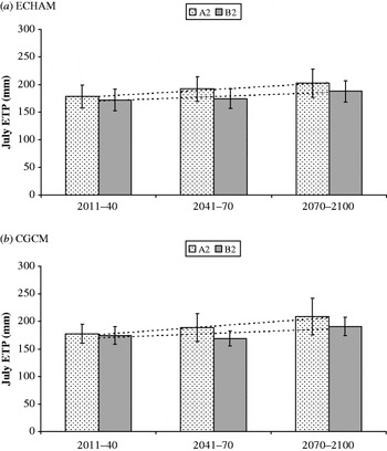
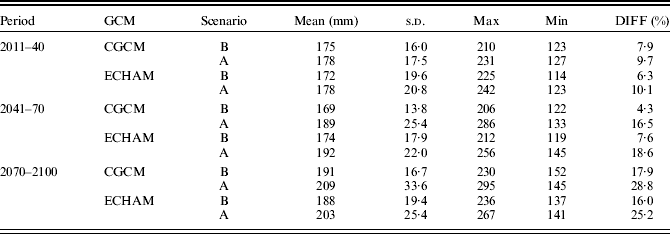
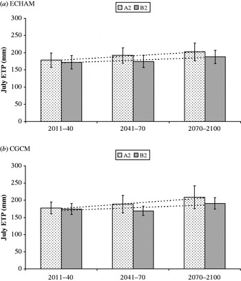
The average July ET for each emission scenario, GCM and period are shown in Fig. 3, with the standard deviations as well as the linear trends obtained in each case. A statistical description of the obtained July ET is shown in Table 1. Besides means and standard deviations, the Table also comprises maximum and minimum values and the 95th percentiles, as indications of extreme values. The percentage difference from the average (measured) ET in the period 1966–2006 is also shown.
Predicted average July ET under different emission scenarios, GCMs and periods. The dashed lines show the linear time trends and the vertical bars indicate the standard deviations at each case.
Means, standard deviations (s.d.), maximum (Max) and minimum (Min) values of the July ET (mm) predicted for Valladolid using different periods, GCM and emission scenarios. The difference (Diff) between these ET predictions and the historical ET mean (162 mm for the period 1966–2006) is expressed as a % of that long-term mean
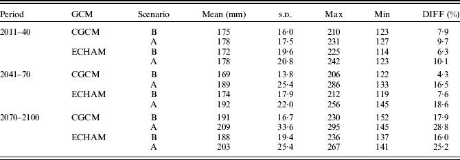
An analysis of variance involving Type III sum of squares assessed the influences of time period, emission scenario and the particular GCM in the results. Both scenario and time periods had most influence on ET estimations during the century (P<0·001). In contrast, the different GCMs had no influence on the results (P>0·05) when all the data were considered. However, those results were not consistent among all the studied periods. The P-values obtained from the analysis of variance of the GCM factor were 0·015 and 0·018 for the 2041–70 and the 2071–2100 periods, respectively. This indicates that the choice of GCM has a significant effect only in the long term. Similarly, the statistical significance of considering emission scenario A or B is higher for the long term (P<0·001) than in the 2011–40 period (P<0·01).
Chi-square and Kolmogorov–Smirnov goodness-of-fit tests to normal probability distribution were conducted for all the data (predictions) at each period (i.e., comprising all scenarios and GCM outputs) as well as for the whole data set. The results indicate that the predicted July ET obtained from the LARS-WG realizations is not normally distributed. Furthermore, Cochran's and Levene's tests of homogeneity of variance indicated that variances within groups were statistically different, which limits the conclusions drawn.
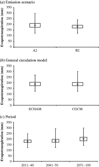
Therefore, non-parametric Kruskal–Wallis tests of the medians were conducted at each of the cases. Figure 4 depicts the Box & Wilker graphs of ET, considering each of the influencing factors. This analysis supported the conclusions obtained from the analysis of variance. The predicted July ET in each of the considered periods is expected to be statistically different. In addition, as can be seen in Fig. 4c, ET medians will be notably higher after 2070, although variability and extreme values after 2040 will be in the same order. The medians, and particularly the variability, of ET are higher under the A2 scenario.
Box and Wilker plots of July ET medians distributed according to the considered emission scenarios, GCM outputs and period. Vertical bars indicate maximum and minimum values.

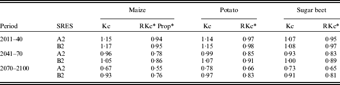
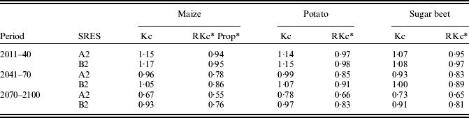
Table 2 shows the crop Kc coefficients of maize, potato and sugar beet, modified according to Eqn (2) for the CO2 concentrations corresponding to each period and SRES. The Table shows also each estimated Kc as a proportion of the currently used coefficients for July. As expected, CO2 effects reduce future Kc in all cases. The variation with respect to currently used Kc is higher for the A2 emission scenario.
Crop Kc coefficients fitted according Eqn (2) to CO2 concentration for each of the considered periods and SRES
* Relative relationship regarding currently used Kc.
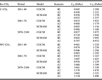
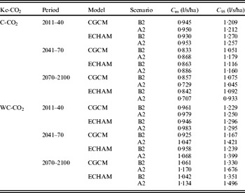
The estimated water supply, following the same procedure used for the designed example, is shown in Table 3. The Table shows also the water supply required to fulfil the evaporative demands of the upper 95th percentile of ET distributions, instead of estimated mean ET values. Calculations include CO2-modified Kc, as well as current Kc coefficients. Estimated water supply is higher if the CO2 effect is ignored.
Calculated water supply needed at average ETs (Cm) and the upper 95th percentile (C95) of the ET distributions for each period, GCM and emission scenario; either incorporation CO2 effects on the crop Kc (C-CO2) or without incorporating it (i.e., using the current Kc coefficient ; WC-CO2)
DISCUSSION
ET is higher for the A2 scenario, as well as the rising rate. July average ET rates are >25% higher than the historical measured averaged for the A2 scenario after 2070, compared to c. 16% increases for the B2 scenario. Furthermore, variability is also higher for the A2 scenario. The variability could be c. 15% at the end of the century, compared with an expected variability of 10% from 2011 to 2040. Maximum values and upper 95th percentiles are very high for all the models and scenarios for 2070–2100. In extreme cases, differences regarding historical ET mean could reach almost 70% by the end of the century.
The ANOVA results obtained from each GCM show that they are not significantly different if all the data are considered, as well as for the 2011–40 period. However, the results from each model are different at the 2041–70 and 2071–2100 periods (P<0·05). Non-parametric tests showed that the outputs from the two different GCMs did not influence the results in 2011–40 or 2071–2100 periods, or when considering the complete data. Nevertheless, as can be seen in Fig. 4b, the estimated variability from CGCM is notably higher than that of ECHAM. Olesen et al. (Reference Olesen, Carter, Díaz-Ambrona, Fronzek, Heidmann, Hickler, Holt, Minguez, Morales, Palutikof, Quemada, Ruiz-Ramos, Rubæk, Sau, Smith and Sykes2007) found that the choice of GCM could be significant for climate change impacts assessments in European agriculture. They considered data from several countries and concluded that regional differences were the most important source of variability. In addition, the ANOVA results of Olesen et al. (Reference Olesen, Carter, Díaz-Ambrona, Fronzek, Heidmann, Hickler, Holt, Minguez, Morales, Palutikof, Quemada, Ruiz-Ramos, Rubæk, Sau, Smith and Sykes2007) indicated also that the emission scenario chosen is the most important statistical source of variation. However, their analysis was based on classical ANOVA, and so assumed that data were normally distributed.
The Kc coefficients are reduced in all cases, but most notably for A2 at the end of the century. This result is consistent with similar studies on the effect of climate change in Spanish agriculture (Guereña et al. Reference Guereña, Ruiz-Ramos, Díaz-Ambrona, Conde and Mínguez2001; Mínguez et al. Reference Mínguez, Ruiz-Ramos, Díaz-Ambrona, Quemada and Sau2007). Table 2 shows only the results of applying Eqn (2) and disregards the propagated errors. However, Kruijt et al. (Reference Kruijt, Witte, Jacobs and Kroon2008) showed that uncertainty related to regression equations is high. Since there are few experimental data for C4 crops, the uncertainty of estimates of maize Kc using Eqn (2) can reach c. 0·50 of the estimated mean. Hence, the results shown in Table 2 must be checked when more data from FACE experiments in C4 crops become available.
Several authors have highlighted a potential increase in irrigation requirements due to global warming, especially using the A2 emission scenario (Elgaali et al. Reference Elgaali, Garcia and Ojima2006; De Silva et al. Reference De Silva, Weatherhead, Knox and Rodriguez-Diaz2007; Rodríguez Díaz et al. Reference Rodríguez Díaz, Weatherhead, Knox and Camacho2007; Gonzalez-Camacho et al. Reference Gonzalez-Camacho, Mailhol and Ruget2008). Those results were obtained considering more than one GCM simulation, but ignoring the eventual effects of CO2 on transpiration.
However, if the CO2 effect on Kc is included, the historical ET exceeds predicted crop water at the end of the century. Comparison of Tables 1 and 2 shows that Kc can be reduced by up to 75% of current values, while increases in mean ET rates are as much as 20%. This would be more apparent using the emission scenario A2, which is associated with a higher predicted concentration of CO2 in the future. Similar results were obtained by Kang et al. (Reference Kang, Zhang, Hu and Zhang2002), Magliulo et al. (Reference Magliulo, Bindi and Rana2003), Triggs et al. (Reference Triggs, Kimball, Pinter, Wall, Conley, Brooks, Lamorte, Adam, Ottman, Mathiass, Leavitt and Cerveny2004), Kim et al. (Reference Kim, Sicher, Bae, Gitz, Baker, Timlin and Reddy2006) and Meza et al. (Reference Meza, Silva and Vigil2008).
The design water supply chosen for the system, considering the historical ET, was 1 litre/s/ha (ITACyL 2007). As shown in Table 3, this supply is generally sufficient to meet the water needs of crops, on average, throughout the century.
As a general conclusion, the irrigation systems designed considering historical maximum demands might be able, on average, to meet future demands for irrigation, even considering climate change. Inclusion or exclusion of CO2 effects in the analysis can influence the results significantly. The increase in CO2 concentrations might, beneficially, cause significant reductions in irrigation demands during the century, but this needs verification. If the effect of increased CO2 concentration on ET is ignored, the system may be slightly under-resourced for the period 2070–2100. The system shortage would be most marked for the A2 emission scenario. The differences between the two scenarios could be up to 10% at the end of the century. More attention should be given to this effect since uncertainty from available data is still high (Kruijt et al. Reference Kruijt, Witte, Jacobs and Kroon2008).
Thus, designers of irrigation systems need to be more aware of FACE experiments results, especially those measuring CO2 effects on crop transpiration. Equally, climate change scientists conducting FACE experiments should appreciate that their results are very relevant to irrigation designs and irrigation planning in the future. Including CO2 effects on Kc changes seems to be essential in estimating future crop water needs.
As already mentioned, the frequency of extreme events, such as heat waves, will increase in Spain and Southern Europe as a result of climate change (Alcamo et al. Reference Alcamo, Moreno, Nováky, Bindi, Corobov, Devoy, Giannakopoulos, Martin, Olesen, Shvidenko, Parry, Canziani, Palutikof, van der Linden and Hanson2007). The upper 95th percentile of ET distributions could be up to 25% higher in the future, as shown in Table 1. Correspondingly, estimated water supply in extreme situations is higher at the end of the century as well. Table 3 indicates that for those July months extremely hot, reaching ET above the upper 95th percentile, the system will be unable to meet the crop water needs, particularly under the A2 emission scenario. The system could function properly for these extreme cases only if the CO2 effect was real, only at the end of the century and only for the A2 emission scenario. The estimated reduction in crop water requirements is higher in that case, which makes the system reliable even in more extreme situations.
Weather variability seems to be the greatest risk for the correct performance of irrigation systems in the medium term (Long et al. Reference Long, Ainsworth, Leakey, Nosberger and Ort2006; Kruijt et al. Reference Kruijt, Witte, Jacobs and Kroon2008). The negative consequences of weather variability have been pointed out already (Katz & Brown Reference Katz and Brown1992; Mearns et al. Reference Mearns, Rosenzweig and Goldberg1997; Reilly et al. Reference Reilly, Tubiello, McCarl and Melillo2001) and the present results also show that variability could be an important risk.
The increase of extreme events associated with climate change could notably increase ET variability. The present results indicated this variability as the main failing risk in irrigation systems that were designed considering historical ET averages. This risk could be more important in the short and medium terms, when the CO2 effect of reducing crop water demand is still not significant. It is advisable that future designs of irrigation systems take into account the variability in ET associated with climate change.
The work conducted in this paper was supported by the EU Proposal ADAGIO (FP6-2005-SSP-5-A).