1. Introduction
Large-eddy simulations (LES) are based on the assumption that small-scale turbulent eddies are more isotropic than the large ones, and are responsible for energy dissipation. Modelling the small scales while resolving the larger eddies may be very effective: first, since most of the momentum transport is due to the large eddies, model inaccuracies are less critical compared with, for instance, Reynolds-averaged Navier–Stokes (RANS) formulations; second, the modelling of the unresolved scales is easier, since they tend to be more homogeneous and isotropic than the large ones, which depend on the specific boundary conditions used to define the flow problem at hand.
The size of the smallest eddies that are resolved in LES is related to the length scale of the smoothing operator, the ‘filter width’, which will be denoted here by
 ${\it\Delta}$
. In this paper we investigate the consequences of relating the filter width (and, therefore, the model length scale) to some fraction of the length-scale representative of the energy- and momentum-carrying eddies, an integral scale of turbulence
 $L$
. The grid size,
 $h$
, should then, ideally, be sufficiently smaller than eddies of size
 ${\it\Delta}$
for these flow features to be represented accurately. The association of a local filter width with a fraction of the local integral scale allows to incorporate in a natural way flow heterogeneities, while keeping the universality assumption of the small turbulent scales intact.
The most commonly used models for the flow physics at the unresolved scales are of eddy-viscosity type: the contribution of the unresolved scales to the resolved momentum transport, the unresolved stresses (often called the ‘subgrid-scale stresses’, but here referred to as ‘subfilter stresses’) is given by
 $$\begin{eqnarray}{\it\tau}_{ij}-\frac{{\it\delta}_{ij}}{3}{\it\tau}_{kk}=-2{\it\nu}_{T}\unicode[STIX]{x1D61A}_{ij}\end{eqnarray}$$
where
 $\unicode[STIX]{x1D61A}_{ij}$
is the resolved strain-rate tensor
 $(\overline{u}_{i,j}+\overline{u}_{j,i})/2$
in terms of partial derivatives of the spatially filtered velocity field
 $\overline{u}_{i}$
. Almost invariably, the eddy viscosity
 ${\it\nu}_{T}$
is determined as the product of a length scale and a velocity scale, and the former is taken to be proportional to the filter width. In many cases the velocity scale is also proportional to the filter width (a prime example is the Smagorinsky–Lilly model (Smagorinsky Reference Smagorinsky1963; Lilly Reference Lilly1967)); the velocity scale can also be obtained from a separate transport equation (Yoshizawa Reference Yoshizawa1982; Ghosal et al.
Reference Ghosal, Lund, Moin and Akselvoll1995) or from a dynamic procedure (Germano et al.
Reference Germano, Piomelli, Moin and Cabot1991) exploiting Germano’s identity (Germano Reference Germano1992). Non-eddy-viscosity models have also been proposed; examples are the mixed model (Bardina, Ferziger & Rogallo Reference Bardina, Ferziger and Rogallo1980) (which contains an eddy-viscosity component of the Smagorinsky type next to Bardina’s similarity model (Bardina et al.
Reference Bardina, Ferziger and Rogallo1980)), regularization models (Geurts & Holm Reference Geurts and Holm2006b
; Geurts, Kuczaj & Titi Reference Geurts, Kuczaj and Titi2008) or tensor-diffusivity models (Leonard & Winckelmans Reference Leonard, Winckelmans, Voke, Sandham and Kleiser1999). In these cases the resulting model also preserves an explicit dependence on
 ${\it\Delta}$
.
The filter width
 ${\it\Delta}$
plays a central role in the modelling of subfilter dynamics, both from the point of view of the method formulation and from that of its practical implementation. Consequently, there has been considerable discussion on its appropriate value. In most cases, the filter width is taken to be proportional to the grid size
 $h$
, i.e.
 ${\it\Delta}=nh$
, where
 $n$
is typically chosen equal to 1 or 2 (McMillan & Ferziger Reference McMillan and Ferziger1979). If the mesh is Cartesian and anisotropic, an appropriate average is used to determine
 $h$
, usually either algebraic or geometric:
 $$\begin{eqnarray}h=(h_{x}h_{y}h_{z})^{1/3}\quad \text{or}\quad h=(h_{x}^{2}+h_{y}^{2}+h_{z}^{2})^{1/2}\end{eqnarray}$$
(where
 $h_{x}$
,
 $h_{y}$
and
 $h_{z}$
are the grid spacings in the three coordinate directions). The best value of
 $n$
has been the subject of some debate. Ghosal (Reference Ghosal1996) discusses the effect of the filter width on modelling and aliasing errors, and concludes that, if second-order accurate differencing schemes are used,
 ${\it\Delta}=8h$
is required to decrease the numerical discretization errors to negligible levels, relative to the contribution of the subfilter model to the fluxes; only if higher-order schemes are used smaller values of
 $n$
can be used. Geurts & Fröhlich (Reference Geurts and Fröhlich2002) reported approximately grid-independent simulation results for a turbulent mixing layer with
 ${\it\Delta}=4h$
, using a fourth-order accurate finite-volume method. Lund (Reference Lund2003) studied the effect of varying
 $n$
within the context of explicit filtering of the nonlinear terms, but concluded that using a high value of
 $n$
is not cost-effective, in the sense that reducing both
 $h$
and
 ${\it\Delta}$
gives more accurate results (compared with unfiltered direct numerical simulation (DNS) results) than reducing
 $h$
with a fixed
 ${\it\Delta}$
, at the same cost. He also observed that the ratio
 ${\it\Delta}/h$
at which convergence is observed depends on the statistical quantity studied. A comprehensive error-landscape study was presented by Meyers, Geurts & Baelmans (Reference Meyers, Geurts and Baelmans2003, Reference Meyers, Geurts and Baelmans2005) for homogeneous, isotropic, decaying turbulence. In such a computational approach a sequence of resolutions
 $N$
and filter widths
 ${\it\Delta}$
is studied to provide an overview of the simulation error that occurs. It was shown that an optimal value of
 $n$
depends on the spatial resolution and the subfilter model adopted. A side-result after such an error-landscape analysis is the identification of an ‘optimal refinement’ strategy which specifies the optimal model parameter as function of resolution.
It must be mentioned that in most cases the filter width is not a well-defined quantity, since the shape of the filter function is not generally known. The implicit use of the discretization to filter the equations is inconsistent, as pointed out by Lund (Reference Lund2003). Even when explicit filtering of the Navier–Stokes (NS) equations is performed (Bose, Moin & You Reference Bose, Moin and You2010; Singh, You & Bose Reference Singh, You and Bose2012), the implicit filtering due to the application of finite differences changes (in an unknown way) the shape of the filter function. Perhaps the only filter that is exactly known and defined is the Fourier cutoff in wave space. If the filter function is unknown the filter width
 ${\it\Delta}$
cannot be defined uniquely. Thus, in the following, we will use
 ${\it\Delta}$
and refer to the filter width, in a loose sense, to indicate the scale of the smallest eddies resolved in the calculation.
Relating the filter width to the mesh size has a simple rationale: the smallest eddy that can potentially be distinguished, in a numerical calculation, has size proportional to the grid; thus, the unresolved eddies are those smaller than the grid (hence, the term ‘subgrid-scale stresses’). This choice, however, carries a number of implications, some of them undesirable.
-
(a) As the grid is refined, the filter width also decreases. This results in the well-known asymptotic behaviour of an LES approaching a DNS as
 $h$
(and, hence,
${\it\Delta}$
) become smaller. This seems poor practice, as grid refinement not only affects discretization errors but also implies an adaptation of the contribution of the model for the unresolved scales. It is unclear how to distinguish model contributions from numerical influences. Moreover, the main motivation to embark on an LES was the infeasibility of DNS in the first place; hence, approximating such an infeasible target using coarse resolutions only may not be optimal (Meyers et al.
Reference Meyers, Geurts and Baelmans2003). Furthermore, performing grid-convergence studies is not straightforward, since many turbulent statistics are filter-dependent (hence, intrinsically grid-dependent). Recently, some studies of grid convergence have been performed by maintaining
${\it\Delta}$
fixed while decreasing
$h$
(Vreman, Geurts & Kuerten Reference Vreman, Geurts and Kuerten1996; Geurts & Fröhlich Reference Geurts and Fröhlich2002; Gullbrand Reference Gullbrand2002; Lund Reference Lund2003; Meyers et al.
Reference Meyers, Geurts and Baelmans2003; Bose et al.
Reference Bose, Moin and You2010).
-
(b) In most calculations the grid is refined in regions of the flow where large gradients are expected. Thus, some intuitive attempt is made to decrease the filter width where the local integral scale is smaller. When complex flows are simulated, however, it may not be possible to know, a priori, where the integral scale decreases (and refine the mesh in these regions). Even in simple wall-bounded flows the relationship between grid size and filter width may not be straightforward. For instance, the two definitions of
$h$
in (1.2) result in very different behaviours of near a solid wall where the wall-normal integral scale behaves as
$L\sim {\it\kappa}y$
, where
${\it\kappa}$
is the von Kàrmàn constant, while those parallel to the wall remain constant. In these regions, typically,
$h_{x},h_{z}\gg h_{y}$
. If the algebraic mean is used,
${\it\Delta}$
(proportional to
$h$
) decreases; if the geometric one is employed, on the other hand,
${\it\Delta}$
remains nearly constant. -
(c) In cases in which adaptive meshes are used with local refinement, sudden variations of the grid size can occur. These result in sharp gradients in the eddy viscosity that can lead to aliasing errors. Moreover, the presence of sharp changes in the filter width is directly associated with commutation errors (which occur when filtering and differentiation do not commute). This problem was studied, among others, by Sullivan, McWilliams & Moeng (Reference Sullivan, McWilliams and Moeng1996), Geurts & Holm (Reference Geurts and Holm2006a ) and Vanella, Piomelli & Balaras (Reference Vanella, Piomelli and Balaras2008), who observed that the filter width must be decoupled from the grid size in the vicinity of an interface between a coarse and a fine mesh. Analyses of the commutator errors were presented in Ghosal & Moin (Reference Ghosal and Moin1995) and van der Bos & Geurts (Reference van der Bos and Geurts2005b ). In addition, theoretical estimates as well as direct evaluation of commutator errors for turbulent flow in a temporal mixing layer were carried out by Geurts (Reference Geurts, Voke, Sandham and Kleiser1999) and van der Bos & Geurts (Reference van der Bos and Geurts2005a ). In the case of considerable non-uniformity and skewness of the filter, the fluxes due to commutator errors were found to be up to 25 % of the subfilter fluxes. Such would arise on non-uniform grids near solid walls when filter width and grid spacing become identical. Non-commuting filters formally induce violation of the conservation of mass and momentum in terms of the filtered velocity field (Geurts et al. Reference Geurts, Vreman, Kuerten, Van Buuren, Chollet, Voke and Kleiser1997). Smooth variation of the filter width was found to suffice to render commutator errors much smaller than subfilter stresses and hence largely remove the need to model these terms directly. A unified solution for subfilter stresses and commutator errors arises from adapting regularization modelling (Geurts & Holm Reference Geurts and Holm2006a ).


Mason & Callen (Reference Mason and Callen1986) attempted to relate the model length scale to the integral scale of the flow for wall-bounded flows. They performed simulations of plane channel flow, and the filter width was assigned as
 $$\begin{eqnarray}{\it\Delta}=\left[\frac{1}{{\it\kappa}(y+y_{o})}+\frac{1}{l_{o}}+\frac{1}{{\it\kappa}(2{\it\delta}-y+y_{o})}\right]^{-1},\end{eqnarray}$$
where
 ${\it\delta}$
is the channel half-width and
 $y_{o}$
is the roughness length of the surface. This prescription matches a constant filter width
 ${\it\Delta}=l_{o}$
in the interior of the channel, to a mixing length
 ${\it\kappa}y$
near the walls.
 $l_{o}$
is taken to be a fraction (between 0.02 and 0.04) of the channel half-width. A strong dependence of the results on
 $l_{o}$
was observed on a fixed mesh. Weaker dependence was observed when
 $l_{o}$
was maintained constant and the grid was refined.
Girimaji and coworkers proposed the partially-averaged Navier–Stokes (PANS) equations (Girimaji Reference Girimaji2006; Girimaji, Jeong & Srinivas Reference Girimaji, Jeong and Srinivas2006), a model that bridges the RANS equations to DNS. In addition to the averaged continuity and momentum conservation equations, a turbulence model (the
 $\mathscr{K}{-}{\it\varepsilon}$
model in the original formulation) is used, and two parameters are introduced,
 $f_{k}$
and
 $f_{{\it\varepsilon}}$
, which measure the amount of turbulent kinetic energy (TKE) and dissipation that the model is expected to provide. In general,
 $f_{{\it\varepsilon}}$
is set to unity, while
 $f_{k}$
determines whether the model is in the RANS regime
 $(\,f_{k}\simeq 1)$
or if some of the turbulence scales are resolved. The values of
 $f_{k}$
used by Girimaji (Reference Girimaji2006), ranging between 0.4 and 1, are much higher than what would be expected in LES (where the small scales typically carry a much lower fraction of the energy).
Menter & Egorov (Reference Menter and Egorov2005, Reference Menter and Egorov2010) also developed a two-equation model that spans RANS and LES. They modified the
 $\mathscr{K}{-}L$
two-equation model, originally proposed by Rotta (Reference Rotta1970) by introducing a length scale that varies locally and resolves the eddies larger than the length scale
 $L$
. Application of the model to a circular cylinder in a cross-flow demonstrated that the model behaves as a RANS model when the boundary layer is attached while the LES behaviour of the model switches on in the massively separated regions. This behaviour is similar to the DES model by Spalart et al. (Reference Spalart, Jou, Strelets, Allmaras, Liu and Liu1997) with the difference that the Menter–Egorov model is formulated independently of the grid and geometry.
In this work we will follow an approach in which the definition of the model length scale
 $\ell$
is directly based on local turbulence quantities characteristic of the flow that is considered. It is emphasized that this natural length-scale distribution within the flow domain is grid-independent; the flow physics are considered completely independent from any numerical element such as spatial discretization method and computational grid. This approach to LES follows the classical partial differential equation (PDE) interpretation of the closed LES equations (Geurts Reference Geurts2003). The mesh size
 $h$
can in our PDE approach be chosen in such a way that the smallest resolved eddy, of size
 ${\it\Delta}$
(which should be related to the model length scale
 $\ell$
), be reproduced accurately by the numerical method. This approach has several potential advantages: grid refinement studies are straightforward and a clear measure of the adequacy of the resolution is provided by the ratio
 ${\it\Delta}/h$
achieved. Grid nesting and local refinement can be performed without any sharp gradients in the eddy viscosity, which will be beneficial in reducing the aliasing errors. This approach will be presented and applied to homogeneous isotropic turbulence (HIT) as well as turbulent channel flow at a range of Reynolds numbers. In this way we establish the practical usability of the formulation, next to its theoretical appeal.
In the following, after introducing the governing equations and describing the numerical scheme and the boundary conditions (§ 2), we will present the model for the unresolved eddies and specify the definition of the length scale and filter width (§ 3); a theoretical analysis of the model will also be carried out. There will be an extensive discussion of possible ways to evaluate the model coefficient, followed by the application of the proposed model to two flows in § 4, i.e. forced HIT (in which the theoretical findings are evaluated numerically), and a turbulent plane channel flow at Reynolds numbers up to
 $\mathit{Re}_{{\it\tau}}=2000$
(based on channel half-width and friction velocity
 $u_{{\it\tau}}$
). Some concluding remarks and recommendations for future work will be presented in § 5.
2. Governing equations and numerical model
In the classical approach to LES, the velocity field is separated into a resolved (large-scale) and a small-scale, unresolved field by a spatial filtering operation (Leonard Reference Leonard1975). The continuity and the Navier–Stokes equations for the resolved field are
 $$\begin{eqnarray}\displaystyle & \displaystyle \frac{\partial \overline{u}_{i}}{\partial x_{i}}=0, & \displaystyle\end{eqnarray}$$
 $$\begin{eqnarray}\displaystyle & \displaystyle \frac{\partial \overline{u}_{i}}{\partial t}+\frac{\partial (\overline{u}_{j}\overline{u}_{i})}{\partial x_{j}}={\it\nu}\frac{\partial ^{2}\overline{u}_{i}}{\partial x_{j}\partial x_{j}}-\frac{\partial {\it\tau}_{ij}}{\partial x_{j}}-\frac{1}{{\it\rho}}\frac{\partial \overline{p}}{\partial x_{i}}+f_{i}. & \displaystyle\end{eqnarray}$$
 $x_{1}$
,
 $x_{2}$
and
 $x_{3}$
are the streamwise, wall-normal and spanwise directions, respectively, also referred to as
 $x$
,
 $y$
and
 $z$
. The resolved velocity components in these directions are, respectively,
 $\overline{u}_{1}$
,
 $\overline{u}_{2}$
and
 $\overline{u}_{3}$
(or
 $\overline{u}$
,
 $\overline{v}$
and
 $\overline{w}$
). In these equations,
 ${\it\tau}_{ij}=\overline{u_{i}u_{j}}-\overline{u}_{i}\overline{u}_{j}$
are the unresolved stresses that constitute the well-known central closure problem in LES. Their modelling will be discussed in the next section.
For HIT, periodic boundary conditions were applied in all directions. To produce sustained turbulence the linear forcing method proposed by Rosales & Meneveau (Reference Rosales and Meneveau2005) was used. The force in the momentum equations (2.2) is given by
 $$\begin{eqnarray}f_{i}=A\overline{u}_{i}\quad \text{with}~A=\frac{\langle 2{\it\nu}\overline{S}^{2}+{\it\tau}_{ij}\unicode[STIX]{x1D61A}_{ij}\rangle _{{\it\Omega},t}}{\langle \overline{u}_{i}\overline{u}_{i}\rangle _{{\it\Omega},t}}\end{eqnarray}$$
where
 $\langle \dots \rangle _{{\it\Omega},t}$
is the average over the entire volume
 ${\it\Omega}$
and time, and
 $\overline{S}=(2\unicode[STIX]{x1D61A}_{ij}\unicode[STIX]{x1D61A}_{ij})^{1/2}$
. The numerator of (2.3) represents the total dissipation rate (viscous and residual) of resolved kinetic energy,
 $\langle \overline{\mathscr{K}}\rangle _{{\it\Omega},t}$
, while the denominator is twice
 $\langle \overline{\mathscr{K}}\rangle _{{\it\Omega},t}$
.
In channel flow, periodic boundary conditions were used in the streamwise and spanwise directions and no-slip boundary conditions in the normal direction. The forcing in the case of channel flow is
 $f_{i}={\it\delta}_{1i}\,f_{p}$
, and
 $f_{p}$
is the pressure gradient, which is adjusted at each time step to maintain a constant flow rate.
The Navier–Stokes equations are discretized using second-order central differences on a staggered grid, and integrated using a fractional step method (Chorin Reference Chorin1968; Kim & Moin Reference Kim and Moin1985). The spatial discretization of the convective terms conserves momentum and energy discretely (Morinishi et al. Reference Morinishi, Lund, Vasilyev and Moin1998). All terms are advanced explicitly in time using a third-order Runge–Kutta method, except (in the channel-flow calculations) for the diffusive term, which is advanced implicitly using a second-order Crank–Nicolson method. The Poisson equation is solved directly by Fourier expansion in the streamwise and spanwise directions (in which the spacing is uniform) followed by an inversion of the resulting tridiagonal matrix at each wavenumber. The code is parallelized using MPI, and has been validated extensively for a variety of turbulent flows (Keating et al. Reference Keating, Piomelli, Balaras and Kaltenbach2004a ,Reference Keating, Piomelli, Bremhorst and Nešić b ; Keating & Piomelli Reference Keating and Piomelli2006).
3. Subfilter-scale model
The use of a grid-independent length scale for subfilter-scale (SFS) modelling of turbulent motions will be illustrated on the basis of the well-known eddy-viscosity approach. In this section we present the formulation of a local turbulence length scale for LES and its incorporation in an eddy-viscosity model. Generalization to other classes of SFS models such as similarity (Bardina et al. Reference Bardina, Ferziger and Rogallo1980) and regularization models (Geurts & Holm Reference Geurts and Holm2006b ) can be pursued analogously.
The unresolved stresses are modelled using an eddy-viscosity approximation (1.1), in which we write the eddy viscosity as
 $$\begin{eqnarray}{\it\nu}_{T}=\left(C_{m}{\it\Delta}\right)^{2}|\overline{S}|=\ell ^{2}|\overline{S}|,\end{eqnarray}$$
where we have introduced a model coefficient
 $C_{m}$
, and the model length scale
 $\ell$
. As mentioned before,
 ${\it\Delta}$
should be a fraction of the local, instantaneous integral scale of turbulence
 $L$
. Mason & Callen (Reference Mason and Callen1986) implemented the same idea by having a constant model length scale in the channel centre, matched to a mixing length near the channel walls (1.3). We wish to generalize this idea and make it applicable to complex flows.
Turbulence models for the RANS equations generally prescribe the integral scale using a velocity scale and a time scale (Speziale Reference Speziale1991). The velocity scale is the square root of the TKE
 $\mathscr{K}=\langle u_{i}^{\prime }u_{i}^{\prime }\rangle /2$
(a prime here denotes a fluctuating quantity, and the bracket an average to which we return momentarily). The time scale can be given by a combination of
 $\mathscr{K}$
and, for instance, the viscous dissipation (Hanjalić & Launder Reference Hanjalić and Launder1972), the pseudo-vorticity (Saffman Reference Saffman1970; Wilcox Reference Wilcox1974) or the vorticity
 ${\it\omega}=\langle {\it\omega}_{i}{\it\omega}_{i}\rangle ^{1/2}$
, where
 ${\it\omega}_{i}={\it\varepsilon}_{ijk}\overline{u}_{j,k}$
, and
 ${\it\varepsilon}_{ijk}$
is the permutation symbol.
Piomelli & Geurts (Reference Piomelli and Geurts2010, Reference Piomelli, Geurts, Kuerten, Geurts, Armenio and Fröhlich2011) proposed a definition of
 $L$
based on TKE and vorticity, to give
 $$\begin{eqnarray}L_{est}=\mathscr{K}^{1/2}/{\it\omega}\quad \Rightarrow \quad \ell \propto \mathscr{K}^{1/2}/{\it\omega}.\end{eqnarray}$$
They used the total vorticity (instead of the fluctuating one) to preserve the property that in a laminar boundary layer the length scale will go to zero. This model was applied to plane-channel flow and temporally developing mixing layers and showed some very promising features: grid convergence was achieved, and the filter width became grid-independent as the mesh was refined; the model correctly predicted the flow behaviour in the near-wall region, and gave more accurate results than existing models, especially on coarse meshes. The model also gave vanishing eddy viscosity in transitional flows and near a solid wall. The asymptotic behaviour near the wall was
 ${\it\nu}_{T}\sim y^{2}$
, close to the exact one,
 ${\it\nu}_{T}\sim y^{3}$
(Germano et al.
Reference Germano, Piomelli, Moin and Cabot1991; Piomelli Reference Piomelli1993).
One shortcoming of the TKE vorticity model was the fact that it used only the resolved part of TKE and vorticity, neglecting the contribution of the unresolved scales. While this approximation may be reasonable for the TKE, which is mostly due to the large scales, it is less justifiable for the vorticity, which depends on the small scales; as the Reynolds number is increased, the neglected contribution of the small scales becomes larger.
To avoid this shortcoming, we propose to define the filter width in terms of an approximation of the integral length scale, which characterizes the large eddies:
 $$\begin{eqnarray}L_{est}=\mathscr{K}^{3/2}/{\it\varepsilon}_{tot},\end{eqnarray}$$
where
 ${\it\varepsilon}_{tot}$
is the dissipation rate of
 $\mathscr{K}$
, given by
 $$\begin{eqnarray}{\it\varepsilon}_{tot}=\langle 2({\it\nu}+{\it\nu}_{sfs})s_{ij}^{\prime }s_{ij}^{\prime }\rangle ,\end{eqnarray}$$
and
 $s_{ij}^{\prime }$
is the fluctuating part of the strain-rate tensor
 $\unicode[STIX]{x1D61A}_{ij}$
. The filter width could then be expressed as a fraction of the integral length scale:
 $$\begin{eqnarray}{\it\Delta}=C_{{\it\Delta}}L_{est}.\end{eqnarray}$$
The inclusion of the contribution of the unresolved scales to the dissipation in (3.4) is expected to be more accurate than (3.2) at high Reynolds numbers; the use of the resolved TKE, as mentioned above, is expected to result in small errors even if the filter width is deep into the inertial range.
To determine quantitatively the error implicit in such assumption, we consider the model spectrum (Pope Reference Pope2000):
 $$\begin{eqnarray}\displaystyle & E(k)=C{\it\varepsilon}^{2/3}k^{-5/3}f_{L}(kL)f_{{\it\eta}}(k{\it\eta}) & \displaystyle\end{eqnarray}$$
 $$\begin{eqnarray}\displaystyle & \displaystyle f_{L}(kL)=\left[\frac{kL}{\left(\left(kL\right)^{2}+6.78\right)^{1/2}}\right]^{11/3} & \displaystyle\end{eqnarray}$$
 $$\begin{eqnarray}\displaystyle & f_{{\it\eta}}(k{\it\eta})=\exp \left\{-5.2\left[\left((k{\it\eta})^{4}+0.40^{4}\right)^{1/4}\right]\right\} & \displaystyle\end{eqnarray}$$
 $C=1.5$
is the Kolmogorov constant and
 $k$
is the wavenumber. We calculate the TKE and dissipation by integrating (3.6)–(3.8) over the entire wavenumber range, to yield the total TKE and dissipation,
 $\widehat{\mathscr{K}}_{tot}$
and
 $\widehat{{\it\varepsilon}}_{tot}$
(a hat here indicates that the quantity is calculated using the model spectrum), or up to a cutoff wavenumber
 $\widehat{K}_{c}={\rm\pi}/{\it\Delta}$
, to obtain the resolved TKE and dissipation,
 $\widehat{\mathscr{K}}_{res}$
and
 $\widehat{{\it\varepsilon}}_{res}$
. Then, we construct three length scales,
 $$\begin{eqnarray}L_{ex}=\widehat{\mathscr{K}}_{tot}^{\,\,3/2}/\widehat{{\it\varepsilon}}_{tot};\quad L_{est}=\widehat{\mathscr{K}}_{res}^{\,\,3/2}/\widehat{{\it\varepsilon}}_{tot};\quad L_{res}=\widehat{\mathscr{K}}_{res}^{\,\,3/2}/\widehat{{\it\varepsilon}}_{res},\end{eqnarray}$$
where
 $L_{ex}\rightarrow L$
as
 $\mathit{Re}_{L}\rightarrow \infty$
. Since the integrals are performed up to a cutoff wavenumber, we are implicitly adopting a Fourier cutoff filter, in which the relationship between cutoff wavenumber and filter width is well defined.
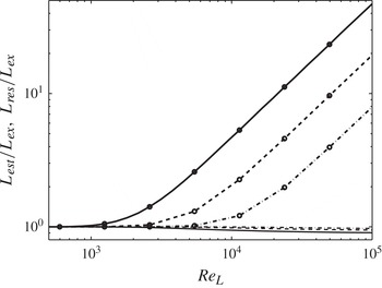
In figure 1 we show the ratio between
 $L_{est}$
,
 $L_{res}$
and the exact integral length
 $L_{ex}$
, for various values of the Reynolds number (based on the integral scale
 $L_{ex}$
and
 $\widehat{\mathscr{K}}_{tot}^{\,\,1/2}$
) and for
 ${\it\Delta}=C_{{\it\Delta}}L_{ex}$
, with
 $C_{{\it\Delta}}=0.005$
, 0.01 and 0.02. Although the use of the resolved TKE (instead of the total one) results in an underestimation of the actual TKE by less than 10 %, the ratio
 $L_{res}/L_{ex}$
departs significantly from unity beyond a critical Reynolds number, which increases as
 $C_{{\it\Delta}}$
is decreased. Using only the resolved dissipation is reasonable at low or moderate Reynolds numbers, but grossly underestimates the dissipation for
 $\mathit{Re}_{L}>10^{4}$
, leading to the significant overestimation of the integral scale. The use of the total dissipation, therefore, appears desirable, and the model (3.3) potentially presents a significant advantage compared with that proposed by Piomelli & Geurts (Reference Piomelli and Geurts2010, Reference Piomelli, Geurts, Kuerten, Geurts, Armenio and Fröhlich2011). In the latter, only the resolved vorticity was used (which would lead to the error observed when
 $L_{res}$
is used), while (3.3) allows for the inclusion of the contribution of the unresolved scales to the dissipation. Modelling errors will still, of course, affect the value of the dissipation; the systematic error associated with neglecting the small-scale contribution to the dissipation is, however, alleviated. This is a crucial advantage of the new formulation and key to this paper: its associated benefits in actual turbulence simulations at high Reynolds numbers will be presented momentarily.
Ratio of integral length scales: line,
 $L_{est}/L_{ex}$
; line with circles,
 $L_{res}/L_{ex}$
; ——,
 $C_{{\it\Delta}}=0.02$
; - - - -,
 $C_{{\it\Delta}}=0.01$
; — ⋅ —,
 $C_{{\it\Delta}}=0.005$
.

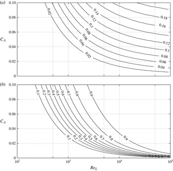
Contours of the ratio of (a) subfilter energy to total energy,
 $\widehat{\mathscr{K}}_{sfs}/\widehat{\mathscr{K}}_{tot}$
, and (b) subfilter dissipation to total dissipation
 $\widehat{{\it\varepsilon}}_{sfs}/\widehat{{\it\varepsilon}}_{tot}$
as a function of
 $\mathit{Re}_{L}$
and the coefficient
 $C_{{\it\Delta}}$
.

With this definition of the length scale, the eddy-viscosity model in (3.1) takes the form
 $$\begin{eqnarray}{\it\nu}_{sfs}=C_{k}^{2}\frac{\mathscr{K}^{3}}{{\it\varepsilon}_{tot}^{2}}|\overline{S}|=\ell ^{2}|\overline{S}|,\end{eqnarray}$$
where all the model constants have been combined into
 $C_{k}$
, and the model length scale is defined as
 $\ell =C_{k}L_{est}=C_{k}\mathscr{K}^{3/2}/{\it\varepsilon}_{tot}$
. We call this the integral length-scale approximation (ILSA) model. The coefficient
 $C_{k}$
(through its dependence on
 $C_{{\it\Delta}}$
) is the parameter that determines the turbulence resolution. A large value of
 $C_{k}$
implies that a large range of turbulent eddies is modelled, a small one corresponds to a calculation in which most of the eddies are resolved. Figure 2 shows the ratio of subfilter to total energy, and subfilter to total dissipation, obtained from the integration of the model spectrum (3.6)–(3.8). In the range of Reynolds numbers and coefficients
 $C_{{\it\Delta}}$
considered, most of the energy (
 ${>}95\,\%$
) resides in the large scales. As expected, as
 $\mathit{Re}_{L}$
is increased for fixed
 $C_{{\it\Delta}}$
, the SFS provide an increasing percentage (approaching 100 %) of the dissipation. Conversely, for constant
 $\widehat{{\it\varepsilon}}_{sfs}/\widehat{{\it\varepsilon}}_{tot}$
,
 $C_{{\it\Delta}}$
approaches 0 as
 $\mathit{Re}_{L}\rightarrow \infty$
, while
 $\widehat{\mathscr{K}}_{sfs}/\widehat{\mathscr{K}}_{tot}$
reaches an asymptotic value.
Figure 2 also suggests a strategy to assign the value of the coefficient: one could require that the SFS contribute a fixed amount of energy or dissipation. This is analogous to the concept of ‘adaptive LES’ proposed by Pope (Reference Pope2004), and also related to the PANS formulation, in that the fraction of energy that one expects the SFS eddies to support can be assigned by the user (in PANS, through the coefficients
 $f_{k}$
and
 $f_{{\it\varepsilon}}$
). Unlike PANS, however, we will not assume that the SFS contribute the entire dissipation, and assign a value for the resolved energy fraction: rather, we will assume that the resolved energy fraction is nearly unity.
The ILSA model defined in (3.10) has a number of features. First, the use of the integral length scale naturally decreases the model length scale in regions of high gradients in which smaller scales may be present. Second, grid convergence studies are straightforward, since refining the grid is formally decoupled from changes in the filter width; only indirect coupling of mesh-spacing and filter width can occur when changing an under-resolved simulation into a properly resolved one in which the local ratio
 ${\it\Delta}/h$
is sufficiently large. Third, the fact that the model length scale does not depend on the grid size should make this approach potentially more accurate in calculations that use adaptive mesh refinement with sharp variations in the local mesh size (Sullivan et al.
Reference Sullivan, McWilliams and Moeng1996; Vanella et al.
Reference Vanella, Piomelli and Balaras2008). Since the integral scale is an average (in the Reynolds sense) quantity, both
 $\mathscr{K}$
and
 ${\it\varepsilon}$
should be averaged to yield the integral scale. Plane averages can be used in flows that are homogeneous in two directions (channel, temporally developing mixing layer, etc.). Lagrangian averages (Meneveau, Lund & Cabot Reference Meneveau, Lund and Cabot1996) appear a natural extension for more complex flows without directions of homogeneity. Using a local formulation, in which the integral length scale is defined instantaneously at each point is an intriguing possibility that deserves consideration; this will not, however, be considered in the present work, in which averages are performed over the homogeneous directions and over time.
To understand the near-wall behaviour of the proposed model we can write
 $$\begin{eqnarray}{\it\nu}_{sfs}\propto \frac{\mathscr{K}^{3}}{({\it\nu}+{\it\nu}_{sfs})^{2}|s^{\prime }|^{4}},\end{eqnarray}$$
where
 $|s^{\prime }|^{2}=2s_{ij}^{\prime }s_{ij}^{\prime }$
. In laminar shear-free regions (3.11) is of the form
 $0/0$
; this technical problem is resolved by adding a small number to the denominator. Near a wall the behaviour is more complex: since
 $u\propto y$
,
 $\mathscr{K}^{3}\propto y^{6}$
, while
 $|s^{\prime }|\propto \text{const.}$
For low Reynolds numbers,
 ${\it\nu}\gg {\it\nu}_{sfs}$
and
 ${\it\nu}_{sfs}\propto \mathscr{K}^{3}\propto y^{6}$
. As
 $\mathit{Re}\rightarrow \infty$
, on the other hand,
 ${\it\nu}\ll {\it\nu}_{sfs}$
and (3.11) yields that
 ${\it\nu}_{sfs}^{3}\propto \mathscr{K}^{3}\propto y^{6}$
, or
 ${\it\nu}_{sfs}\propto y^{2}$
. Neither of those two limits is the correct
 ${\it\nu}_{sfs}\propto y^{3}$
one (Germano et al.
Reference Germano, Piomelli, Moin and Cabot1991). Nevertheless, the viscosity vanishes quite rapidly, and requires no explicit correction, as will be shown later.
Finally, we point out that, in this formulation, the terms ‘subgrid-scale model’ and ‘subgrid-scale stresses’ are not appropriate, since the unresolved eddies may turn out to be larger than the grid. In the following, therefore, we will refer to ‘subfilter scale (SFS) eddies, stresses’. Note that this terminology is already used, especially in the combustion and meteorological communities, and is discussed by Pope (Reference Pope2000).
4. Results and discussion
It was mentioned above that various possibilities exist to determine the coefficient
 $C_{k}$
. Therefore, we will begin by describing the method we chose (§ 4.1). The application of the new SFS model to forced HIT, and to turbulent channel flow at
 $\mathit{Re}_{{\it\tau}}$
up to 2000 is presented subsequently (§§ 4.2 and 4.3). Finally, in § 4.4 we compare results of the new modelling approach to standard models in literature, and discuss the computational cost of the proposed model.
4.1. Determination of
$C_{k}$

There are a number of ways in which the relation between the filter width and the local integral length scale can be specified. The model coefficient
 $C_{k}$
can, for example, be specified by the user based on the computational resources available. Alternatively, one could find an optimum value for
 $C_{k}$
that minimizes the total simulation error in the prediction of a set of selected quantities that may be known from experiments, theoretical considerations or DNS. For instance, Piomelli & Geurts (Reference Piomelli and Geurts2010, Reference Piomelli, Geurts, Kuerten, Geurts, Armenio and Fröhlich2011) required that the coefficient minimizes the error in the prediction of the skin-friction coefficient,
 $C_{f}=2{\it\tau}_{w}/{\it\rho}U_{b}^{2}$
(where
 ${\it\tau}_{w}$
is the wall stress,
 ${\it\rho}$
the fluid density and
 $U_{b}$
the average velocity in the channel), which is known from experimental data.
An alternative is to use an internal measure of the simulation resolution to determine
 $C_{k}$
. For this study, therefore, we define two measures of the contribution to the transport by the SFS. The first is the ratio of SFS dissipation to the total dissipation, defined as (Meyers et al.
Reference Meyers, Geurts and Baelmans2003)
 $$\begin{eqnarray}s_{{\it\varepsilon}}=\frac{\langle {\it\varepsilon}_{sfs}\rangle }{\langle {\it\varepsilon}_{sfs}\rangle +\langle {\it\varepsilon}_{{\it\nu}}\rangle }=\frac{\langle 2{\it\nu}_{sfs}\unicode[STIX]{x1D61A}_{ij}\unicode[STIX]{x1D61A}_{ij}\rangle }{\langle 2({\it\nu}+{\it\nu}_{sfs})\unicode[STIX]{x1D61A}_{ij}\unicode[STIX]{x1D61A}_{ij}\rangle }.\end{eqnarray}$$
Geurts & Fröhlich (Reference Geurts and Fröhlich2002) and Meyers et al. (Reference Meyers, Geurts and Baelmans2003) observed that for large filter-width-to-grid ratios,
 $s_{{\it\varepsilon}}$
depends mostly on
 ${\it\Delta}$
. An appropriate choice of the averaging operator might be case-dependent; here, we have averaged over the entire domain and time.
A second measure is the SFS contribution to the Reynolds stresses. This measure should, however, take into account the fact that the SFS stress model, in the eddy-viscosity formulation, does not include the SFS energy. Therefore, the simplest coordinate-invariant measure of the Reynolds stresses is the second invariant of the anisotropic part of the Reynolds stress tensor. Let
 $$\begin{eqnarray}\unicode[STIX]{x1D619}_{ij}^{a}=\overline{u}_{i}^{\prime }\overline{u}_{j}^{\prime }-{\it\delta}_{ij}\frac{\overline{u}_{k}^{\prime }\overline{u}_{k}^{\prime }}{3};\quad {\it\tau}_{ij}^{a}={\it\tau}_{ij}-{\it\delta}_{ij}\frac{{\it\tau}_{kk}}{3},\end{eqnarray}$$
where
 $\overline{u}_{i}^{\prime }=\overline{u}_{i}-\langle \overline{u}_{i}\rangle _{hd,t}$
is the resolved turbulent fluctuation, difference between resolved and mean velocity (averaged over homogeneous directions and time). We define
 $$\begin{eqnarray}s_{{\it\tau}}=\left[\frac{\langle {\it\tau}_{ij}^{a}{\it\tau}_{ij}^{a}\rangle }{\langle (\unicode[STIX]{x1D619}_{lm}^{a}+{\it\tau}_{lm}^{a})(\unicode[STIX]{x1D619}_{lm}^{a}+{\it\tau}_{lm}^{a})\rangle }\right]^{1/2}.\end{eqnarray}$$
Once a desired level of
 $s_{{\it\varepsilon}}$
or
 $s_{{\it\tau}}$
is assigned, the value of
 $C_{k}$
that ensures that the SFS model yields the desired subfilter activity can be found by performing a series of calculations on coarse grids; production calculations can subsequently be performed with higher reliability on finer meshes. With this procedure,
 $C_{k}$
becomes a user-defined resolution parameter, related to the cost of the calculation, and to the computational power available. Large values of
 $s_{{\it\varepsilon}}$
or
 $s_{{\it\tau}}$
result in large values of
 $C_{k}$
, corresponding to fairly coarse LES in which most of the energy transfer is modelled, and/or a large proportion of the Reynolds stresses are unresolved. Such calculations can be expected to converge on coarse grids. Small values of
 $s_{{\it\varepsilon}}$
or
 $s_{{\it\tau}}$
, conversely, will result in small values of
 $C_{k}$
, and finer meshes will be required. In the limit
 $s\rightarrow 0$
, the filter width vanishes and the DNS limit is recovered as the mesh is refined.
To minimize the number of coarse-grid calculations required to determine
 $C_{k}$
, the error-minimization technique based on the successive inverse polynomial interpolation (SIPI) procedure, as proposed by Geurts & Meyers (Reference Geurts and Meyers2006) to optimize the Smagorinsky constant, is used. The SIPI method is based on the definition of a measure
 ${\it\phi}$
of the difference between some target quantity and the LES prediction of this quantity. Geurts & Meyers (Reference Geurts and Meyers2006), for instance, performed simulations of HIT, and based the definition of
 ${\it\phi}$
on the TKE. The method consists of performing three LES on a coarse mesh, for values of
 $C_{k}$
that bracket the optimum (one evaluation is always performed with
 $C_{k}=0$
, one with a fairly large value of
 $C_{k}$
, the third with an intermediate value). We then construct an interpolating parabola, and find its minimum, which is used for the next evaluation of
 ${\it\phi}$
. The interpolation is then repeated using three pairs
 $[C_{k},{\it\phi}(C_{k})]$
(including the newest one) that result in a parabola with an upwards concavity. A new minimum is found and a new error evaluation carried out. This procedure resulted in an accurate identification of the minimum with typically less than six error evaluations. The cost of the whole procedure is small, given that the SIPI test runs are performed on a mesh that is much coarser than that used for the production runs. The use of the coarse mesh is made possible by the fact that the integral length scale (3.3) (and, hence,
 $\ell$
and
 ${\it\Delta}$
) is representative of the largest turbulence scales, and is expected to be predicted reasonably well even by coarse calculations. Obviously, the latter requirement does implicitly set some lower bound on the coarsest resolutions that actually can be adopted in such a set of SIPI test runs. In the applications considered here, the overhead created by these SIPI runs was found to be less than 5 %.
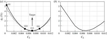
Figure 3 demonstrates the application of SIPI on a channel flow using the proposed model at
 $\mathit{Re}_{{\it\tau}}=950$
on a coarse grid (
 $48\times 65\times 48$
). The parameters of the simulation are discussed later. For this case
 ${\it\phi}$
is based on subfilter activity
 $s_{{\it\varepsilon}}$
:
 $$\begin{eqnarray}{\it\phi}_{s}\hspace{2.22198pt}\%=100\times \left|s_{{\it\varepsilon}}-s_{tgt}\right|^{2}\end{eqnarray}$$
where
 $s_{tgt}$
is set to 0.23; this value would be typical of a well-resolved LES of a wall-bounded flow; the sensitivity of the results to the target value will be examined later. The first three calculations were performed with
 $C_{k}=0.000$
(point (i)),
 $C_{k}=0.009$
(point (ii)) and
 $C_{k}=0.0045$
(point (iii)). The parabola constructed from these three points yields a minimum for
 $C_{k}=0.007$
. A fourth calculation was carried out with this value, and the next parabola created by points (ii), (iii) and (iv); it also has a minimum at
 $C_{k}=0.007$
, indicating this value as the target value. In total four simulations were performed to optimize
 $C_{k}$
. The optimum value obtained directly by sampling
 ${\it\phi}_{s}$
in a number of cases was also verified by performing nine simulations (figure 3
b), and is the same as that found using SIPI.
SIPI optimization for plane channel flow at
 $\mathit{Re}_{{\it\tau}}=950$
with subfilter activity
 $s_{{\it\varepsilon}}$
as quantity to be optimized with target value
 $s_{tgt}=0.23$
and grid
 $48\times 65\times 48$
. (a) Error optimization based on SIPI; the first polynomial has been constructed using points (i)–(iii) (——); the second using (ii)–(iv) (- - - -). (b) Error obtained from nine simulations with varying values of
 $C_{k}$
.

As mentioned, all of the averages required to evaluate the SFS ratios,
 $s_{{\it\varepsilon}}$
and
 $s_{{\it\tau}}$
, are carried out over the entire computational domain and time. A single value of the coefficient
 $C_{k}$
obtains; the model length scale
 $\ell$
, however, may vary if the TKE and dissipation are only averaged in homogenous directions (as will be the case in the plane channel flow). This choice is by no means unique, and is made here to simplify the initial applications of the model. Its effects and limitations will be discussed in § 4.3. More local averages can also be used, and are the subject of ongoing work.
4.2. Forced HIT
We first performed simulations of HIT, with Reynolds number (based on
 $\mathscr{K}^{1/2}$
and the integral scale
 $L$
)
 $\mathit{Re}_{L}=250$
. To achieve a steady state, a force was added to the right-hand side of the momentum equation. Following Rosales & Meneveau (Reference Rosales and Meneveau2005)
 $A=0.1333$
in (2.3). The domain size was
 $2{\rm\pi}\times 2{\rm\pi}\times 2{\rm\pi}$
, and the initial condition was a solenoidal isotropic velocity field with random phases and the energy spectrum:
 $$\begin{eqnarray}E_{T}(k)=\frac{16}{\sqrt{{\rm\pi}/2}}\frac{u_{o}^{2}k^{4}}{k_{o}^{5}}\exp \left(-\frac{2k^{2}}{k_{o}^{2}}\right),\end{eqnarray}$$
where
 $u_{o}=1$
is the initial root-mean-square (r.m.s.) velocity, and
 $k_{o}=20$
the wavenumber where the spectrum is maximum. These input parameters correspond to one of the three DNS cases performed by Rosales & Meneveau (Reference Rosales and Meneveau2005) using a pseudo-spectral method. Note that, with the forcing defined in (2.3), at steady state
 $A=\langle \overline{{\it\varepsilon}}_{tot}\rangle _{{\it\Omega},t}/2\langle \mathscr{\overline{K}}\rangle _{{\it\Omega},t}$
, yielding
 $L=\langle \mathscr{\overline{K}}\rangle _{{\it\Omega},t}^{1/2}/2A$
. The DNS simulation by Rosales & Meneveau (Reference Rosales and Meneveau2005) showed that the TKE reaches an asymptotic state around 0.3; therefore, we expect
 $L\simeq 2.05$
.
Here
 $C_{k}$
was determined by choosing a target value of the subfilter activity
 $s_{{\it\varepsilon},tgt}=0.15$
. Simulations were then performed on a coarse grid with
 $32^{3}$
points, and the optimum value of
 $C_{k}$
was found using SIPI; only 5 simulations were required to find that
 $C_{k}\simeq 0.006$
gave
 $s_{{\it\varepsilon},tgt}=0.15$
. To evaluate the sensitivity of the results to increasing the range of eddies that are resolved, we also performed the optimization using
 $s_{{\it\varepsilon},tgt}=0.3$
, a value expected to give a more significant contribution of the SFS to the momentum transport. The coefficient increased to 0.010.
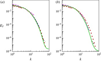
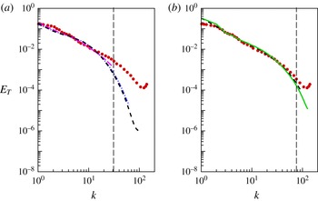
Figure 4(a,b) show the energy spectra
 $E_{T}(k)$
calculated, for
 $C_{k}=0.006$
and
 $C_{k}=0.010$
, using different grids. Several observations can be made; in both figures the energy spectra collapse onto each other for
 $128^{3}$
grid points when
 $C_{k}=0.006$
, and
 $32^{3}$
when
 $C_{k}=0.010$
. This is consistent with the observations by Geurts & Fröhlich (Reference Geurts and Fröhlich2002) and Meyers et al. (Reference Meyers, Geurts and Baelmans2003) in which, for higher subfilter activity, grid convergence was achieved at coarser resolution. The value
 $L\simeq 2.05$
is also achieved to good approximation using both
 $C_{k}$
values when
 $64^{3}$
grid points are used (not shown). Finally, we observe that when
 $C_{k}=0.006$
, smaller eddies (higher wavenumbers) are resolved while the use of a higher
 $C_{k}$
value tends to increase the contribution of the subfilter model, resulting in a strong attenuation of the predicted spectra at high wavenumbers (figure 4
b). For the higher value of
 $C_{k}$
, the spectrum decays more rapidly at high wavenumbers. Since the DNS data are not filtered, this results in a larger difference with the reference data.
Total energy spectra at grid resolutions of
 $---$
 $32^{3}$
, — ⋅ —
 $64^{3}$
, - - - -
 $128^{3}$
and ——
 $192^{3}$
with: (a)
 $s_{{\it\varepsilon},tgt}=0.15$
and
 $C_{k}=0.006$
; (b)
 $s_{{\it\varepsilon},tgt}=0.3$
and
 $C_{k}=0.010$
. The ● shows DNS (Rosales & Meneveau Reference Rosales and Meneveau2005).

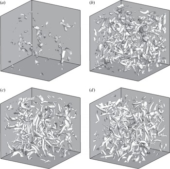
In figure 5 we compare the flow structures obtained, for different grid resolutions, for the
 $C_{k}=0.010$
case. The eddies are visualized using isosurfaces of the second invariant of the velocity gradient tensor,
 $\unicode[STIX]{x1D64C}$
(Hunt, Wray & Moin Reference Hunt, Wray and Moin1988; Dubief & Delcayre Reference Dubief and Delcayre2000):
 $$\begin{eqnarray}\unicode[STIX]{x1D64C}=-\frac{1}{2}\frac{\partial \overline{u}_{i}}{\partial x_{j}}\frac{\partial \overline{u}_{j}}{\partial x_{i}}.\end{eqnarray}$$
We observe progressively smaller structures being resolved as the mesh is refined, and also more finely detailed appearance of the resolved eddies. At coarse grids the contribution of numerical discretization errors is quite significant. Conversely, beyond a resolution of
 $128^{3}$
the global visual impression of the flow appears quite similar, suggesting the start of convergence to a grid-independent LES. For the lower value of
 $C_{k}$
(not shown) smaller scales appear, as expected.
Isosurfaces of
 $\unicode[STIX]{x1D64C}=5.00$
for
 $C_{k}=0.010$
: (a)
 $32^{3}$
points; (b)
 $64^{3}$
points; (c)
 $128^{3}$
points; (d)
 $192^{3}$
points.

We also performed simulations at a higher Reynolds number,
 $\mathit{Re}_{L}=4490$
. The spectra are shown in figure 6, for
 $s_{{\it\varepsilon}}=0.84$
(resulting in
 $C_{k}=0.006$
) and
 $s_{{\it\varepsilon}}=0.44$
(which gives
 $C_{k}=0.0015$
). Grid-convergence appears to set in beyond
 $128^{3}$
and
 $256^{3}$
grid points, respectively. The correspondence between the spectrum obtained here, with an undefined filter function, and the model spectrum coupled with a sharp Fourier cutoff discussed before is only approximate; however, we can remark, with reference to figure 2(b), that, at this Reynolds number,
 $s_{{\it\varepsilon}}=0.84$
corresponds to
 $C_{{\it\Delta}}\simeq 0.05$
; the filter width is approximately 20 times smaller than the length scale
 $L_{est}$
. The corresponding wavenumber is approximately
 $k_{{\it\Delta}}\simeq 31$
(approximately 77 for
 $s_{{\it\varepsilon}}=0.44$
), and is indicated by a dashed line in the figure. The LES results match the DNS data well up to wavelengths
 $\simeq 2{\it\Delta}$
. Near the cutoff the spectra decay considerably more rapidly, reflecting the high value of
 $s_{{\it\varepsilon}}$
, which causes the model to be very dissipative. Compared with a Smagorinsky model, in which the eddy viscosity is given by
 $$\begin{eqnarray}{\it\nu}_{smag}=(C_{s}h)^{2}|\overline{S}|,\end{eqnarray}$$
with
 $C_{s}\simeq 0.17{-}0.23$
, the present model gives higher dissipation by a factor
 $(C_{k}L_{est}/C_{s}h)^{2}$
. For the grid-converged simulation, with
 $h=2{\rm\pi}/192\simeq 0.016L_{est}$
, this implies that the dissipation predicted by the present model is over three times larger than that of the Smagorinsky model. Choosing a smaller value of the SFS activity,
 $s_{{\it\varepsilon}}=0.44$
results in a wider range of scales in agreement with the DNS data; however, a finer mesh (
 $256^{3}$
grid points) is required to obtain a similar level of grid-converged data; again, eddies of size
 ${>}2{\it\Delta}$
appear accurately captured.
Total energy spectra at grid resolutions
 $---$
 $64^{3}$
, — ⋅ —
 $128^{3}$
, - - - -
 $192^{3}$
and ——
 $256^{3}$
with
 $\mathit{Re}_{L}=4490$
and: (a)
 $s_{{\it\varepsilon},tgt}=0.84$
and
 $C_{k}=0.006$
. (b)
 $s_{{\it\varepsilon},tgt}=0.44$
and
 $C_{k}=0.0015$
. The ● shows DNS (Rosales & Meneveau Reference Rosales and Meneveau2005).

This study highlights an important feature of this SFS model: the fact that the coefficient
 $C_{k}$
is really a user-defined parameter, determined by the SFS activity level chosen. The larger
 $s_{{\it\varepsilon}}$
(or any other measure of the SFSs used), the larger the coefficient and the more significant the contribution of the unresolved scales. As
 $C_{k}$
(and, consequently,
 $\ell$
) are increased, a coarser grid is sufficient to resolve eddies of size comparable to the filter width, but modelling errors are expected to increase as well. An optimal value of the SFS activity may be case-dependent; in the present case, the LES was found to be accurate for scales larger than
 $2{\it\Delta}$
, independent of the value of
 ${\it\Delta}$
that is implied by the definition of
 $\ell$
chosen by the user.
It should be observed that, for
 $C_{k}=0.006$
, i.e.
 $C_{{\it\Delta}}\approx 0.05$
, nearly 10 % of the TKE resides in the unresolved scales (figure 2
a). Approximating
 $\mathscr{K}$
in (3.10) with
 $\mathscr{K}_{res}$
may, therefore, result in errors in
 ${\it\nu}_{sfs}$
, particularly since this viscosity scales with
 $\mathscr{K}^{3}$
. To verify the significance of these errors, three additional simulations were performed. First, the exact value of
 $L$
(obtained from the DNS data) was used; second, we considered a case in which the TKE from the DNS was used in the numerator of (3.10); finally,
 $\mathscr{K}_{sfs}$
was estimated as (Yoshizawa Reference Yoshizawa1986)
 $$\begin{eqnarray}\mathscr{K}_{sfs}=0.0886(C_{{\it\Delta}}L_{est})^{2}|\overline{S}|,\end{eqnarray}$$
and was added to
 $\mathscr{K}_{res}$
in the numerator of (3.10). The results of the four simulations were within 2 % of each other, indicating that neglecting the SFS contribution to the TKE should not give significant errors when the SFSs responsible for less than 10 % of the TKE itself.
4.3. Plane channel flow
Channel flow simulations were performed at
 $\mathit{Re}_{{\it\tau}}=950$
and 2000. The domain size is
 $6{\it\delta}\times 2{\it\delta}\times 3{\it\delta}$
in the streamwise, wall-normal and spanwise directions, respectively. While Piomelli & Geurts (Reference Piomelli and Geurts2010, Reference Piomelli, Geurts, Kuerten, Geurts, Armenio and Fröhlich2011) determined
 $C_{k}$
by minimizing the error in the prediction of skin friction coefficient
 $C_{f}$
, which is known from correlation of experimental data (Dean Reference Dean1978), we chose
 $C_{k}$
to achieve a desired level of the subfilter activity
 $s_{{\it\varepsilon}}$
. The relationship of the chosen measure to others (the amount of Reynolds shear stresses or TKE provided by the model, for instance) will be discussed later.
Figure 3 showed the error minimization for channel flow at
 $\mathit{Re}_{{\it\tau}}=950$
and grid size
 $48\times 65\times 48$
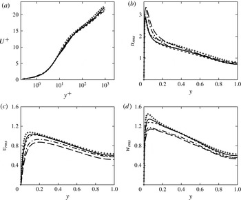
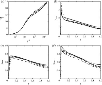
illustrating the effectiveness of the SIPI procedure. Figure 7 shows the mean velocity profile (in wall units) and the turbulence intensities obtained at various grid resolutions. Approximate convergence appears with
 $48\times 65\times 48$
grid points for the mean velocity, while
 $128\times 129\times 128$
grid points are required to obtain near grid-independent Reynolds stresses. The fact that the mean-flow statistics can be predicted reasonably accurately with only
 $48\times 65\times 48$
grid points (corresponding to
 ${\rm\Delta}x^{+}\simeq 119$
and
 ${\rm\Delta}z^{+}\simeq 60$
) is rather surprising: with this resolution the quasi-streamwise vortices in the wall layer cannot be resolved adequately, and LES is not expected to be accurate. This issue will be discussed further later.
Turbulence statistics for
 $\mathit{Re}_{{\it\tau}}=950$
and
 $C_{k}=0.007$
: (a) mean velocity; (b)
 $u_{rms}$
; (c)
 $v_{rms}$
; (d)
 $w_{rms}$
;
 $---$
 $48\times 65\times 48$
grid points; — ⋅ —
 $64\times 97\times 64$
grid points; - - - -
 $128\times 129\times 128$
grid points; ——
 $192\times 193\times 192$
grid points;
 $+$
DNS (Hoyas & Jiménez Reference Hoyas and Jiménez2006).

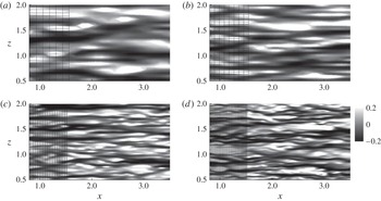
Figure 8 shows contours of streamwise velocity fluctuations obtained with four grids at Reynolds number
 $\mathit{Re}_{{\it\tau}}=950$
. One can observe how refining the mesh results in improved resolution of finer scales, as expected. This grid-refinement study shows that there is very little difference between the results obtained at the two finer meshes. Apparently, for these grids,
 $\ell$
does not change much with resolution, as the integral scale is well-approximated throughout the domain. The smallest resolved eddies that result from the choice
 $C_{k}=0.007$
can be represented reasonably well using
 $128\times 129\times 128$
grid points.
Contours of
 $u$
-velocity fluctuations at
 $y^{+}=11$
superposed on the underlying grid with
 $\mathit{Re}_{{\it\tau}}=950$
and
 $C_{k}=0.007$
: (a)
 $48\times 65\times 48$
, (b)
 $64\times 97\times 64$
, (c)
 $128\times 129\times 128$
and (d)
 $192\times 193\times 192$
grid points.

We also conducted simulations at
 $\mathit{Re}_{{\it\tau}}\simeq 2000$
. The SIPI procedure was carried out on a
 $64\times 97\times 64$
grid using the estimate for subfilter activity based on the dissipation, and a target value
 $s_{tgt}=0.23$
. More refined calculations were subsequently carried out with the value of
 $C_{k}=0.005$
that was obtained from the SIPI algorithm. The turbulence statistics are shown in figure 9, and again demonstrate improved agreement with the DNS data as the mesh is refined while keeping
 $C_{k}$
fixed. This indicates that with the filter-width definition based on flow physics, as proposed here, the convergence to a grid-independent LES can be pursued effectively. At proper (sufficiently low)
 $C_{k}$
the grid-independent LES results will show close agreement with DNS data. As
 $C_{k}\rightarrow 0$
, the DNS limit would be achieved when the grid is refined.
Turbulence statistics for
 $\mathit{Re}_{{\it\tau}}=2000$
and
 $C_{k}=0.005$
: (a) mean velocity; (b)
 $u_{rms}$
; (c)
 $v_{rms}$
; (d)
 $w_{rms}$
; — ⋅ —
 $64\times 97\times 64$
grid points;
 $---$
 $128\times 129\times 128$
grid points; - - - -
 $192\times 193\times 192$
grid points; ——
 $256\times 257\times 256$
grid points;
 $+$
DNS (Hoyas & Jiménez Reference Hoyas and Jiménez2006).

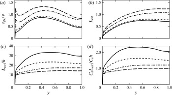
Profiles of several quantities related to the SFS model are shown in figure 10. Figure 10(a) shows the ratio of the eddy viscosity and the molecular viscosity. Some dependence on the grid resolution can be observed on coarse grids as the eddy viscosity converges with grid refinement. This dependence on resolution, however, is much weaker than what would be seen in a classical model of the Smagorinsky type, in which the viscosity depends on
 $h^{2}$
; in the present case the grid resolution is changed by a factor of 4 in each direction between coarsest and finest simulations, which would result in a decrease of the Smagorinsky eddy viscosity by approximately a factor of 16. The eddy viscosity as defined in this paper only decreases by 33 % over the entire range of under-resolved to approximately grid-independent resolutions. Also, the two finest grids give well-converged results for
 ${\it\nu}_{sfs}$
despite the fact that the grid size is different by 50 %. The near-wall behaviour, as expected, is proportional to
 $y^{6}$
, steeper than the theoretical prediction of
 $y^{3}$
.
Profiles of: (a) SFS eddy viscosity; (b) estimated integral scale
 $L_{est}$
; (c) ratio
 $L_{est}/h$
; and (d) ratio
 $C_{k}L_{est}/C_{S}h$
; channel flow,
 $\mathit{Re}_{{\it\tau}}=950$
and
 $C_{k}=0.007$
;
 $---$
 $48\times 65\times 48$
grid points; — ⋅ —
 $64\times 97\times 64$
; - - - -
 $128\times 129\times 128$
; ——
 $192\times 193\times 192$
grid points.

Figure 10(b,c) show the integral length scale
 $L_{est}$
and its ratio to the grid size. First, we observe a rapid rise of
 $L_{est}$
near the wall followed by a more gradual increase in the channel core. As the mesh is refined the prediction of
 $\mathscr{K}$
and
 ${\it\varepsilon}_{tot}$
becomes more accurate, which results in changes in
 $L$
and
 ${\it\nu}_{sfs}$
; a nearly grid-converged value of
 $L$
is reached for the
 $128\times 129\times 128$
grid. The length scale
 $L_{est}$
is of the order of the channel half-width in the core of the flow, reflecting the expected size of the eddies there. The mixing length
 $\ell =-\langle u^{\prime }v^{\prime }\rangle /|\text{d}U/\text{d}y|^{2}$
, in the core of the channel, is approximately equal to
 $0.15{\it\delta}$
, of the same order as
 $L_{est}$
. At this resolution, 20 grid points are required to resolve
 $L_{est}$
(as shown by the ratio
 $L_{est}/h$
in figure 10
c), at least in the channel core.
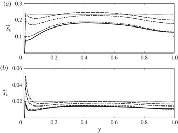
We have chosen, in this paper, to consider a global average of the SFS activity measures. This choice implies that, in inhomogeneous flows, the actual SFS contribution may be higher or lower than the target in different regions of the flow. To understand better the consequences of this choice, in figure 11 we show profiles of a surrogate measure of the SFS activity, plane by plane. This measure is defined as
 $$\begin{eqnarray}\widetilde{s}_{{\it\varepsilon}}=\frac{\langle {\it\varepsilon}_{sfs}\rangle _{xzt}}{\langle {\it\varepsilon}_{tot}\rangle _{xzt}}\frac{s_{{\it\varepsilon}}}{\displaystyle \int _{0}^{h}\frac{\langle {\it\varepsilon}_{sfs}\rangle _{xzt}}{\langle {\it\varepsilon}_{tot}\rangle _{xzt}}\,\text{d}y}\end{eqnarray}$$
where
 $\langle \cdot \rangle _{xzt}$
indicates averaging over wall-parallel planes and time, whereas
 $\langle \cdot \rangle$
indicates averaging over the entire volume (and time). The second term in (4.9) ensures that the average of
 $\widetilde{s}_{{\it\varepsilon}}$
is
 $s_{{\it\varepsilon}}$
. A similar expression defines
 $\widetilde{s}_{{\it\tau}}$
. The figure shows that throughout most of the channel the SFS activity is nearly constant. On the coarse grid (on which the SIPI procedure was carried out) its average value is very close to the target one; on finer grids it is somewhat lower: the grid-converged value of the integral scale is slightly higher than that predicted on the coarse grid (figure 10
d), and on the fine mesh the resolved eddies have a higher-than-expected contribution to the momentum and energy transport. The local SFS activity measures show significant variations only near the wall, for
 $y<0.1{-}0.2~(y^{+}<100{-}200)$
. This result indicates that in calculations of attached boundary layers (especially if wall models are used, in which the first grid point is located in the logarithmic layer) the use of global averaging may be adequate. On the other hand, in flows including separation or other non-equilibrium effects, use of a more local measure of SFS activity may be more suitable. Within that contest (and, in particular, in wall-modelled LES, in which the viscous dissipation is negligible compared with that supplied by the SFSs), we point out that
 $s_{{\it\tau}}$
is a better indicator than
 $s_{{\it\varepsilon}}$
. First, as
 $\mathit{Re}\rightarrow \infty$
one loses much sensitivity when
 $s_{{\it\varepsilon}}$
is used to determine
 $C_{k}$
. Second, requiring that the SFS contribution to the dissipation be equal to
 $s_{{\it\varepsilon}}$
at each point implies that
 ${\it\nu}_{sfs}={\it\nu}/(1-s_{{\it\varepsilon}})$
everywhere as well (whereas with the present approach, this is true only on average). Such a model cannot be expected to be accurate in most flows.
Profiles of plane-averaged SFS activity measures, defined in (4.9): (a)
 $\widetilde{s}_{{\it\varepsilon}}$
; (b)
 $\widetilde{s}_{{\it\tau}}$
;
 $---$
 $48\times 65\times 48$
grid points; — ⋅ —
 $64\times 97\times 64$
; - - - -
 $128\times 129\times 128$
; ——
 $192\times 193\times 192$
grid points. The thin dotted line shows the target value.

Note that the filter width
 ${\it\Delta}=C_{{\it\Delta}}L$
is unknown: the constant
 $C_{{\it\Delta}}$
does not need to be determined as part of the simulation algorithm. The model coefficient
 $C_{k}$
also accounts for the (unknown) constant of proportionality for the time scale. One can estimate
 $C_{{\it\Delta}}$
, however, from figure 2, assuming that the turbulence is isotropic near the centre of the channel. The Reynolds number based on
 $L$
and the turbulence intensity
 $\mathscr{K}^{1/2}$
is approximately 800 in this region, and the subfilter activity calculated at grid convergence is approximately 0.17; figure 2 indicates that these values correspond to
 $C_{{\it\Delta}}\simeq 0.06$
. The filter width is, therefore, smaller than the integral scale by a factor of 15–20 (similar to the values observed for the simulations of HIT discussed before). For the finest mesh, in which
 $L/h\simeq 30$
(figure 10
c), this gives a ratio
 ${\it\Delta}/h\simeq 1.5{-}2$
, which is consistent with earlier observations of subfilter resolutions
 ${\it\Delta}/h$
that would be required to achieve nearly grid-independent numerical solutions (Vreman, Geurts & Kuerten Reference Vreman, Geurts and Kuerten1994; Lund Reference Lund2003). Another estimate of the ratio between filter width and grid size can be obtained by comparing the quantity
 $C_{k}L$
with the analogous quantity used in the Smagorinsky model,
 $C_{s}h$
. As is the case for
 $C_{k}$
,
 $C_{s}$
also includes the constant of proportionality for the time scale. The ratio between the two quantities is shown in figure 10(d). In the channel core this ratio is approximately equal to 1.5 for the
 $128\times 129\times 128$
grid, increasing to 2 for the more refined grid.
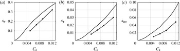
Figure 12 shows the variation of the two measures of subfilter activity defined above in (4.1) and (4.3) with
 $C_{k}$
. We also include a third quantity that measures the SFS contribution to the shear stress,
 $$\begin{eqnarray}s_{uv}=\frac{\left\langle {\it\nu}_{sfs}\unicode[STIX]{x1D61A}_{12}\right\rangle }{\left\langle -\overline{u}^{\prime }\overline{v}^{\prime }+{\it\nu}_{sfs}\unicode[STIX]{x1D61A}_{12}\right\rangle }.\end{eqnarray}$$
While this measure of SFS activity is not generally applicable, being coordinate-dependent, and difficult to generalize to complex geometries, it is useful to relate the measures introduced earlier in the literature to
 $s_{uv}$
, which gives a direct measure of the contribution of the SFSs to momentum transport. The figure shows, first, that the range of
 $s_{{\it\varepsilon}}$
considered (between 0 % and 40 %) corresponds to an SFS contribution to the total shear stress of less than 10 %; the corresponding values of
 $s_{{\it\tau}}$
are under 5 %. As we already observed, on fine grids all of the metrics considered have lower values than those estimated on the coarse mesh for the SIPI procedure used to assign
 $C_{k}$
. Thus, the grid-converged calculations resolve more eddies than expected; indicating that the procedure used to evaluate
 $C_{k}$
is conservative.
Measures of SFS activity; channel flow,
 $\mathit{Re}_{{\it\tau}}=950$
: (a)
 $s_{{\it\varepsilon}}$
; (b)
 $s_{{\it\tau}}$
(c)
 $s_{uv}$
; line,
 $48\times 65\times 48$
grid points; line with symbols,
 $128\times 129\times 128$
grid points.

It is possible also to choose the value of
 $C_{k}$
that optimizes the prediction of some quantity known experimentally. This is predicated on the availability of prior knowledge, and is effective only if the quantity of interest is not strongly dependent on the small scales, since the SIPI procedure is performed on a coarse grid. Piomelli & Geurts (Reference Piomelli and Geurts2010, Reference Piomelli, Geurts, Kuerten, Geurts, Armenio and Fröhlich2011), for instance chose the value of
 $C_{k}$
that minimized the error in the prediction of the skin-friction coefficient,
 $C_{f}$
. While we believe that the use of an internal measure such as
 $s_{{\it\tau}}$
is preferable, we also observe that the values of
 $C_{k}$
chosen here are close to the value that optimizes the prediction of
 $C_{f}$
. On the coarse mesh, in fact, the minimum
 $C_{f}$
is obtained for
 $C_{k}=0.0061$
, close to the value chosen for fine simulations (
 $C_{k}=0.007$
).
Next, we examined the sensitivity of the numerical results to the value of
 $C_{k}$
chosen. We performed simulations on the
 $128\times 129\times 128$
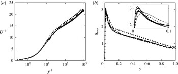
grid, using coefficients ranging from 0.005 to 0.012, corresponding to SFS contributions to the dissipation ranging between 10 % and 33 % (as evaluated on the fine grid) and to the shear stress between 1 % and 5 %. For SFS dissipation between 10 % and 25 % of the total we observe no difference in the mean velocity profiles (figure 13
a) and little difference in the r.m.s. turbulence intensities (figure 13
b; the other components have similar behaviours). When the filter width is increased so that the subfilter eddies contribute over 30 % of the dissipation, we begin to observe errors in the buffer region (see the inset in the figure). In particular, the point of maximum
 $u_{rms}$
moves away from the wall (from
 $y^{+}\simeq 30$
for
 $C_{k}=0.012$
to 13 for
 $C_{k}=0.005$
), and the region of the peak becomes wider, indicating an overestimated diffusion due to a slightly overestimated eddy viscosity. From figure 2, one can estimate that this case corresponds to a filter width
 ${\it\Delta}\simeq 0.07{-}0.1L$
, substantially larger than that corresponding to
 $C_{k}=0.007$
. Even with such a large filter width, however, the differences with the DNS data are surprisingly small.
Profiles of (a) mean velocity and (b)
 $u_{rms}$
; for
 $\mathit{Re}_{{\it\tau}}=950$
; ——
 $C_{k}=0.005$
;
 $\cdots \cdots$
 $C_{k}=0.007$
; - - - -
 $C_{k}=0.009$
; — ⋅ —
 $C_{k}=0.012$
;
 $128\times 129\times 128$
grid points.

4.4. Comparison with other models and cost considerations
We next compare the present model with the dynamic eddy-viscosity model (Germano et al.
Reference Germano, Piomelli, Moin and Cabot1991; Lilly Reference Lilly1992), which is in widespread use. We used the plane-averaged formulation with both grid and test filter widths proportional to the grid size, and performed calculations of the channel flow at
 $\mathit{Re}_{{\it\tau}}=950$
using both a coarse grid (with
 $48\times 65\times 48$
points) and a refined one using
 $128\times 129\times 128$
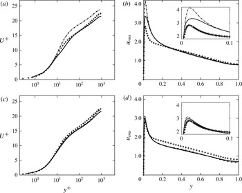
points. Figure 14 compares the mean velocity profiles and the streamwise r.m.s. turbulence intensity,
 $u_{rms}$
. First, the present model, on the coarsest mesh, gives results in surprisingly good agreement with the DNS, while the dynamic model results in an incorrect prediction of the near-wall flow, with an overestimation of the intercept of the logarithmic layer and an excessively high peak of
 $u_{rms}$
, both due to a 12 % underestimation of the wall stress. On a finer grid, on the other hand, both models give similar results. With
 $C_{k}=0.007$
, the SFS eddies are expected to contribute between 16 % and 23 % of the dissipation, and 2 %–4 % of the Reynolds shear stresses (figure 12).
Profiles of (a,c) mean velocity and (b,d)
 $u_{rms}$
for
 $\mathit{Re}_{{\it\tau}}=950$
; —— present model,
 $C_{k}=0.007$
; — ⋅ — dynamic eddy-viscosity model;
 $+$
DNS (Hoyas & Jiménez Reference Hoyas and Jiménez2006); (a,b)
 $48\times 65\times 48$
grid points; (c,d)
 $128\times 129\times 128$
grid points.

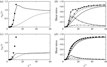
Figure 15 shows that, on the coarse mesh, the present model yields an eddy viscosity that is much larger than that predicted by the dynamic model. This balances the inability of the resolved scales to transport momentum at the appropriate rate: the fluctuation contours shown in figure 8 show streaks of much larger scale than physical, and a more quiescent flow. Thus, the contribution of the SFS to the Reynolds stresses is enhanced (figure 15 b), and exceeds that of the resolved scales in the viscous and buffer layers. In fact, the total Reynolds stress (sum of resolved and SFS components) may be excessively high in the buffer region; the mean velocity gradient must, in that region, be lower, to satisfy the momentum balance; this phenomenon is noticeable in figure 14(a). With the dynamic model, on the other hand, the subfilter stresses are insufficient to balance the unresolved momentum, and the mean velocity gradient must increase to close the momentum balance, leading to the high intercept of the logarithmic layer. On the fine mesh, on the other hand, the dynamic model gives accurate results indicative of the high fidelity achieved at such resolutions.
Profiles of (a,c) eddy viscosity and (b,d) shear stress; channel flow,
 $\mathit{Re}_{{\it\tau}}=950$
. —— Present model,
 $C_{k}=0.007$
; - - - - dynamic eddy-viscosity model; ●
 $\mathscr{K}{-}{\it\omega}$
turbulence model in (a). (a,c):
 $48\times 65\times 48$
grid points. (b,d):
 $128\times 129\times 128$
grid points. For the shear stress figures: lines: resolved stress; lines with squares: SFS stress; lines with circles: total Reynolds stress.

SFS models usually require the energy- and momentum-transporting eddies to be resolved to give accurate results. On the coarse mesh, such is not the case, and the dynamic model cannot be expected to be accurate. The model proposed here, on the other hand, has some features of a RANS turbulence model, through the definition of the integral scale. Figure 15(a) shows the eddy-viscosity obtained for this case by solving the RANS equations with the
 $\mathscr{K}{-}{\it\omega}$
turbulence model (Wilcox Reference Wilcox1993). In the viscous and buffer layers the present model yields virtually the same eddy viscosity as that predicted by the RANS turbulence model. At finer resolution the present model behaves like a standard SFS model, yielding a much lower viscosity than the
 $\mathscr{K}{-}{\it\omega}$
model. It is not to be expected, however, that this behaviour could extrapolate to cases in which
 $s_{{\it\varepsilon}}\rightarrow 1$
: unlike the PANS approach, which solves explicitly an equation for the unresolved TKE, the present model requires that
 $\mathscr{K}_{tot}\simeq \mathscr{K}_{res}$
. Even on the coarse mesh, the resolved eddies support 95 % of the shear stress, integrated over the entire channel (figure 12
c). Presumably, they will support roughly the same percentage of TKE, leading to an accurate prediction of the dissipation length. For
 $s_{{\it\varepsilon}}=0.3$
and
 $s_{{\it\tau}}=0.03$
errors in the prediction of the r.m.s. fluctuations become more significant, even on the fine mesh; these values may approach the limit of applicability of the present model.
An important issue to be considered when developing SFS models is their cost. The model proposed here, in terms of computational cost, is comparable to the Smagorinsky model, and significantly cheaper than dynamic models that require 60 % more CPU time per time step and grid point due to the repeated filtering operations required. The proposed model requires, of course, five or six precursor simulations to determine a reliable estimate of the optimum value of the coefficient
 $C_{k}$
. Since they are performed on a grid that is much coarser than that used for production runs, however, this overhead is not excessive. Tables 1 and 2 show the details of the simulation cost using the proposed SFS model and other models, respectively, for the
 $\mathit{Re}_{{\it\tau}}\simeq 1000$
case; all of the simulations were run for
 $10{\it\delta}/u_{{\it\tau}}$
on eight 2.52 GHz Sparc64 VII processors.
Simulation cost for channel flow at
 $\mathit{Re}_{{\it\tau}}\simeq 1000$
using the proposed SFS model on 8 processors.

Simulation cost for channel flow at
 $\mathit{Re}_{{\it\tau}}\simeq 1000$
using 8 processors and other commonly used models.

The cost of the simulations on the fine mesh for the present model was only 6 % higher compared with a simulation using the Smagorinsky model, and nearly 20 % lower than the dynamic model. The precursor simulations, which were performed on a much coarser grid added only 4 % to the total cost. Including the cost of the precursor simulations, the present model is only marginally more expensive than the Smagorinsky model, and less costly than the dynamic model. These considerations depend to a very large extent on the algorithm used: the present code has a very efficient direct solver for the Poisson equation, which requires a fraction of the total CPU time per step; in codes in which less efficient solvers are used, especially in complex geometries, the Poisson solution may require a much larger fraction of the CPU time, and the cost of the SFS model evaluation may not be a significant consideration.
5. Conclusions
We have proposed a new definition of the length scale to be used in a SFS model, based not on the grid size, as is common practice, but on turbulence quantities. The filter width is defined as a fraction of the local integral length scale
 $L$
, which is approximated as the ratio between the square root of the resolved TKE and the total (sum of resolved and SFS) dissipation. The model coefficient,
 $C_{k}$
, represents a turbulence resolution parameter, which determines what fraction of TKE or dissipation is resolved. The model length scale can be loosely related to the filter width, i.e. the size of the smallest eddy resolved by the LES. Based on its definition, we call it the ILSA model.
The coefficient
 $C_{k}$
in the new model can be determined by specifying the desired contribution of the unresolved scales to either the momentum flux or the energy flux between resolved and unresolved scales. In all cases the determination of
 $C_{k}$
can be carried out on a rather coarse grid, using any error minimization procedure. The one we chose, the SIPI, proposed for a similar problem by Geurts & Meyers (Reference Geurts and Meyers2006) converged to the minimum in five or six function evaluations.
The ILSA model coefficient
 $C_{k}$
is not determined based on physical considerations (as is the case, for instance, in the Smagorinsky–Lilly model (Smagorinsky Reference Smagorinsky1963; Lilly Reference Lilly1967)). It is, instead, derived from a user-defined level of flow resolution. Using the SIPI approach
 $C_{k}$
can be determined once a desired value of a measure of the SFS activity is assigned. Large values of the SFS contribution to the momentum and energy transport result in large filter widths, and simulations that can be performed on coarse grids (but resolve a narrower range of scales). Requiring a smaller SFS contribution, conversely, results in smaller length scales and associated filter widths, that require finer meshes (and a higher cost) in exchange for smaller errors. We have performed calculations in which the SFSs contribute between 15 % and 84 % of the SFS dissipation, in isotropic turbulence and plane channel, to illustrate this point. Although the relation is not rigorous due to the ambiguity of the definition of the filter function in practical applications, in most cases, for grid-independent calculations, the model length scale was approximately 2–4 times the filter width
 ${\it\Delta}$
.
In practice, the chosen value of SFS activity would depend on the available computational power. HIT (and, in particular, some analogue of figure 2) can be used for guidance. The new approach provides a systematic algorithmic framework for optimizing model parameters in relation to computational resources and/or the level of desired flow resolution.
The proposed definition of
 ${\it\nu}_{sfs}$
is, in principle, grid-independent. In practice, as the grid is refined, a more accurate prediction of TKE results in a slight decrease of the integral length
 $L_{est}$
. The decrease, however, is much smaller than that observed when
 ${\it\Delta}$
is taken to be proportional to the grid size. The fact that the integral length scale depends on the resolved TKE, which can be predicted reasonably well even on coarse grids, plays a favourable role in the mild grid-dependence of
 ${\it\nu}_{sfs}$
and also makes it possible to evaluate
 $C_{k}$
on coarse grids with good accuracy. The resulting model is computationally very efficient. Moreover, as the grid is refined, the LES do not tend towards the DNS limit; this allows the straightforward performance of grid-independence studies.
The ILSA model has been tested in HIT and plane channel flow, with results that are as good or better than standard models. One feature of the proposed model that was observed is its accurate prediction of the flow in cases in which the grid is too coarse to resolve the momentum-transporting eddies accurately; the model appears to have a hybrid RANS/LES character, in these circumstances, that results in improved prediction of the flow statistics.
Possible improvements of the model would include a more localized formulation, in which the coefficient
 $C_{k}$
is not everywhere constant. Alternative ways to evaluate it (without precursor simulations) should also be considered. Some of these issues are the subject of ongoing investigations.
Acknowledgements
This research was supported by the Natural Sciences and Engineering Research Council (NSERC) under the Discovery Grant program. The authors thank the High Performance Computing Virtual Laboratory (HPCVL), Queen’s University site, for the computational support. U.P. also acknowledges the support of the Canada Research Chairs Program. The authors thank the Referees for many stimulating observations, and Ingrid Bergman for inspiring the model’s acronym.