1. Introduction
Disperse multiphase systems are a common occurrence, and hence of great relevance, in both natural and industrial settings. Fundamental questions with regard to these systems arise in the context of their non-trivial rheological behaviour, and in relation to estimating the rates of transport of mass or heat (scalar) between the different phases. We consider a scenario where the disperse and continuous phases are Newtonian liquids of the same density, with the ratio of the disperse (
 $\hat {\mu }$
) to continuous (
 $\mu$
) phase viscosities denoted by
 $\lambda$
. When the disperse phase (drop) volume fraction is small, interactions between the different disperse phase constituents can be neglected, and the problem reduces to a single Newtonian drop in an ambient Newtonian fluid undergoing a shearing flow. Further, for neutrally buoyant drops with sizes (
 $a$
) small compared with the characteristic flow scale (say
 $L$
), an arbitrary shearing flow appears as an unbounded linear one at leading order in
 $a/L$
. The small drop size also implies that viscous effects are dominant, and that the Reynolds numbers for both the fluid motion inside and outside the drop, defined as
 $Re = \dot {\gamma } a^2/\nu$
and
 $\hat {Re} = \dot {\gamma }a^2/\hat {\nu }$
, are therefore small; here,
 $\dot {\gamma }$
is a scale for the ambient shear rate, and
 $\nu$
and
 $\hat {\nu }$
are the ambient and drop kinematic viscosities, respectively. In general, for the drop to remain spherical, interfacial tension must dominate ambient viscous stresses, and this requires that the dimensionless parameter quantifying the relative strengths of the two, the capillary number
 $Ca = \mu \dot {\gamma } a /\sigma$
(
 $\sigma$
being the coefficient of interfacial tension), be small.
In this work, we examine a weakly deformed drop in an ambient hyperbolic planar linear flow in the Stokesian regime, the focus being on the drop-deformation-induced alteration of the exterior streamline topology. The geometry of both interior and exterior streamlines is known to profoundly influence transport characteristics in the convection-dominant limit, corresponding to large Péclet numbers, and the role of the interior streamline topology in this regard has been examined in an independent effort (Singeetham et al. Reference Singeetham, Thampi and Subramanian2024). Drop deformation depends on both
 $Ca$
and
 $\lambda$
, and the validity of the weak deformation assumption requires either a large interfacial tension (
 $Ca \ll 1$
,
 $\lambda \sim O(1)$
) as already mentioned above, or a large drop viscosity (
 $\lambda \gg 1$
,
 $\lambda Ca \gtrsim O(1)$
) for ambient linear flows with vorticity that allow for a tank-treading motion of the deformed interface at steady state. Our focus here is on the former small-
 $Ca$
limit.
1.1. Scalar transport from spherical particles and drops in linear flows: the role of streamline topology
We begin with a detailed overview of the literature pertaining to the streamline pattern around a spherical (undeformed) drop or a particle in ambient planar linear flows. Cox, Zia & Mason (Reference Cox, Zia and Mason1968) analysed the streamline pattern around a neutrally buoyant rigid sphere in an ambient simple shear flow, for
 $Re = 0$
, finding a region of closed streamlines around the rotating sphere. The significance of closed exterior streamlines became known from the work of Acrivos (Reference Acrivos1971) who showed, for the above scenario, that the non-dimensional scalar transport rate from the sphere (the Nusselt number
 $Nu$
) plateaus at a finite value for
 $Pe \gg 1$
; here,
 $Pe = \dot {\gamma }a^2/D$
is the Péclet number denoting the relative importance of convection and diffusion, with
 $D$
being the scalar diffusivity. The above studies were extended to the one-parameter family of planar linear flows by Poe & Acrivos (Reference Poe and Acrivos1976), who showed that closed streamlines exist around the rotating sphere for all cases except planar extension, in which case the sphere does not rotate; the parameter characterizing planar linear flows is
 $\hat {\alpha } \in [-1,1]$
with
 $\hat {\alpha } = -1$
,
 $0$
and
 $1$
corresponding to solid-body rotation, simple shear and planar extension, respectively. For simple shear flow in particular, the aforementioned closed streamline region is infinite in extent within the flow-vorticity plane. Poe & Acrivos (Reference Poe and Acrivos1976) also showed, for all cases with a closed streamline region, that
 $Nu$
again plateaus to an
 $\hat {\alpha }$
-dependent value for
 $Pe \gg 1$
; as expected, this limiting value diverges for
 $\hat {\alpha } \rightarrow 1$
. Closed streamlines therefore lead to diffusion-limited transport, in contrast to the continued enhancement expected for an open-streamline topology, owing to boundary-layer-driven transport at large
 $Pe$
; in this latter case,
 $Nu$
increases as
 $Pe^{{1}/{3}}$
for
 $Pe \rightarrow \infty$
for rigid spherical particles. Powell (Reference Powell1983) extended the work of Cox et al. (Reference Cox, Zia and Mason1968) in analysing both the interior and exterior streamline topologies for a neutrally buoyant spherical drop (
 $Ca = 0$
) in an ambient planar linear flow. Unlike a solid particle, the author found that the existence of a closed streamline region in the exterior now depends on both
 $\hat {\alpha }$
and
 $\lambda$
, with such a region arising only for
 $\lambda \gt \lambda _c(\hat {\alpha }) = 2 \hat {\alpha } / (1 - \hat {\alpha })$
; also see Krishnamurthy & Subramanian (Reference Krishnamurthy and Subramanian2018a
). The threshold viscosity ratio
 $\lambda _c(\hat {\alpha })$
diverges for
 $\hat {\alpha } \rightarrow 1$
so that, even for a drop, all streamlines remain open in planar extension regardless of
 $\lambda$
. In contrast,
 $\lambda _c(0) = 0$
, so a closed streamline region exists in simple shear flow for any non-zero
 $\lambda$
, and remains infinite in extent within the flow-vorticity plane.
Closed streamlines are a consequence of Stokesian reversibility. Reversibility constraints are no longer applicable in the presence of inertia, that is, when the Reynolds number, either
 $Re$
or
 $\hat {Re}$
(for a drop), is finite. Subramanian & Koch (Reference Subramanian and Koch2006a
,Reference Subramanian and Kochb) analysed the effect of weak inertia (
 $Re \ll 1$
) on the streamline topology around a rigid sphere in an ambient planar linear flow with
 $\hat {\alpha } \lt 1$
, and found the originally closed streamlines to be replaced by ones that come in from infinity, tightly spiral around the rotating sphere and eventually move off to infinity. The emergence of open spiralling streamlines in the exterior eliminates the diffusion-limited transport that prevails in the Stokesian limit. For any non-zero
 $Re$
, and for sufficiently large
 $Pe$
such that
 $Re Pe \gg 1$
, the said authors found
 $Nu \propto (Re Pe)^{{1}/{3}}$
, a prediction confirmed in later simulations (Yang et al. Reference Yang, Zhang, Koch and Yin2011). It is worth mentioning that earlier efforts (Poe & Acrivos Reference Poe and Acrivos1975; Mikulencak & Morris Reference Mikulencak and Morris2004), which attempted to include inertial effects, had erroneously assumed closed streamlines to persist at finite
 $Re$
, likely motivated by the two-dimensional scenario involving a circular cylinder where closed streamlines cannot open up, despite the onset of inertial effects, on account of incompressibility (Robertson & Acrivos Reference Robertson and Acrivos1970a
; Kossack & Acrivos Reference Kossack and Acrivos1974).
The effect of inertia on the exterior streamline topology for a neutrally buoyant spherical drop, suspended in a planar hyperbolic linear flow, was first analysed by Krishnamurthy & Subramanian (Reference Krishnamurthy and Subramanian2018b
) who found that, much like a rigid sphere, fluid inertia opens up the closed streamlines for
 $\lambda \gt \lambda _c(\hat {\alpha })$
. An analysis of scalar transport leads to
 $Nu \propto (Re Pe)^{{1}/{2}}$
for
 $Re \ll 1, RePe \gg 1$
, corresponding to the leading-order convection being driven by the finite-
 $Re$
spiralling streamlines; note that there exists the usual boundary-layer-driven enhancement for
 $\lambda \lt \lambda _c(\hat {\alpha })$
with
 $Nu \propto Pe^{{1}/{2}}$
for
 $Pe \gg 1$
(Krishnamurthy & Subramanian Reference Krishnamurthy and Subramanian2018a
). The geometry of the spiralling streamlines for a drop is more complicated, with each turn of a near-surface spiralling streamline resembling a Jeffery orbit (a spherical ellipse) with an
 $\hat {\alpha },\lambda$
-dependent aspect ratio, rather than being circular as for a rigid sphere. The analysis of scalar transport in Krishnamurthy & Subramanian (Reference Krishnamurthy and Subramanian2018b
) also showed the existence of a second critical value,
 $\lambda = \lambda _{c2}(\hat {\alpha })$
, demarcating distinct spiralling-streamline regimes: (i) the ‘single-wake’ regime where all near-surface streamlines spiral in from infinity along the vorticity axis, and spiral out in the vicinity of the flow-gradient plane; and (ii) the ‘bifurcated-wake’ regime where near-surface streamlines spiral in both along the vorticity axis, and in the neighbourhood of the flow-gradient plane, and then spiral out along a pair of intermediate directions symmetrically disposed about the plane of shear. This change in the spiralling-streamline topology led to a minimum in the
 $N\!u$
-surface at the transition between the single and bifurcated-wake regimes (Krishnamurthy & Subramanian Reference Krishnamurthy and Subramanian2018b
).
1.2. Drops in shearing flows: deformation, breakup and streamline topology
While inertia is the only source of irreversibility for a solid particle, for a drop, one also has irreversible interfacial forces coming into play when the drop deforms (non-zero
 $Ca$
), and that drive the drop towards sphericity regardless of the sense of the ambient shear. There have been several studies on deformed drops in an ambient linear flow and we briefly survey these efforts, before moving on to a discussion of the streamline topology around a deformed drop; some of the results mentioned below are used for validating the boundary integral (BEM) computations discussed in § 3.3.
Geoffrey Ingram Taylor first determined the steady state drop deformation in simple shear flow (Taylor Reference Taylor1932), and in planar extension (Taylor Reference Taylor1934). In the first effort, Taylor considered both the limit of a dominant interfacial tension (
 $Ca, \lambda Ca \ll 1$
), and that of a dominant drop viscosity (
 $\lambda , \lambda Ca \gg 1$
), although the latter limit was more restrictive than need be. For small
 $Ca$
, the drop deforms into an ellipsoid with its longest axis aligned with the ambient extension, consistent with symmetry arguments that require the deformation to be linear in the ambient rate of strain tensor. For
 $\lambda Ca \gg 1$
, linearity no longer holds, and the deformed drop aligns along the flow direction instead. The implication of these findings is that the inclination of the deformed drop with respect to the flow direction is a function of
 $\lambda Ca$
, decreasing from
 ${\pi }/{4}$
for
 $\lambda Ca \ll 1$
, to
 $0$
for
 $\lambda Ca \gg 1$
. This was confirmed by Cox (Reference Cox1969) who also analysed the transient dynamics of alignment, showing that the approach towards the steady
 ${\pi }/{4}$
-alignment for
 $\lambda Ca \ll 1$
was monotonic, while that towards near-flow-aligned orientations for
 $\lambda Ca \gg 1$
had an oscillatory character, with damped shape oscillations, having a frequency of
 $O(\dot {\gamma })$
, preceding eventual alignment. The relaxation time derived in the analysis of Cox (1969) was incorrect, as pointed out (and corrected) by Rallison (Reference Rallison1980), although the principal features pertaining to the drop dynamics remain unchanged. An important conclusion from the effort of Cox (1969) is the singular nature of the miscible limit (
 $Ca = \infty$
), in which case almost any initial shape leads to persistent undamped oscillations, with there being no steady state for simple shear flow (and, more generally, for any of the planar linear flows with vorticity); the only exception being the trivial scenario where the initial configuration is identical to the stationary one – for simple shear, this is the flow-aligned configuration derived by Taylor (Reference Taylor1932) for
 $\lambda Ca = \infty$
. For planar extension alone, a miscible drop will be stretched out to infinity regardless of
 $\lambda$
(leading to eventual breakup). These features of miscible drop dynamics in an ambient linear flow, have been confirmed by Tucker and coworkers (Wetzel & Tucker Reference Wetzel and Tucker1999, Reference Wetzel and Tucker2001).
Following Cox (1969), Frankel & Acrivos (Reference Frankel and Acrivos1970) calculated the drop deformation to second order in
 $Ca$
, which was further extended by Barthes-Biesel & Acrivos (Reference Barthes-Biesel and Acrivos1973) to
 $O(Ca^3)$
. Even though both perturbation expansions were developed for small values of a general deformation parameter
 $\epsilon$
which could equal either
 $Ca$
or
 $1/\lambda$
, solutions were found only for the former case since, for
 $\epsilon = 1/\lambda$
, one needs to account for terms in the convected (Jaumann) derivative that jump order when
 $\lambda Ca \sim O(1)$
(Rallison Reference Rallison1980). Much later, Greco (Reference Greco2002) recognized that the small-
 $C\!a$
corrections to the leading-order spherical-drop disturbance field involved a characteristic quadratic combination of the rate of strain and vorticity tensors, and used this insight to simplify the calculation of higher-order terms. Later studies of Vlahovska and coworkers (Vlahovska et al. Reference Vlahovska, Loewenberg and Blawzdziewicz2005, Reference Vlahovska, Blawzdziewicz and Loewenberg2009) have extended the small-deformation analysis to surfactant-laden drops where the Marangoni number (
 $Ma$
) enters as an additional parameter; in the limit of a clean interface (
 $Ma \rightarrow 0$
), the authors’ results improve upon those of Barthes-Biesel & Acrivos (Reference Barthes-Biesel and Acrivos1973). Finally, following the suggestion of Rallison (Reference Rallison1980), Oliveira & Cunha (Reference Oliveira and daCunha2011, Reference Oliveira and daCunha2015) calculated the higher-order corrections in the large-
 $\lambda$
limit, albeit for asymptotically large rather than order-unity values of
 $\lambda Ca$
. While the discussion above has focused on earlier analytical efforts, there have also been numerical investigations of drop deformation and breakup, originally using the BEM technique (Rallison Reference Rallison1978; Stone & Leal Reference Stone and Leal1989, Reference Stone and Leal1990; Kennedy & Pozrikidis Reference Kennedy and Pozrikidis1994; Kwak & Pozrikidis Reference Kwak and Pozrikidis1998), and more recently, using other methods (Li, Renardy & Renardy Reference Li, Renardy and Renardy2000; Amani et al. Reference Amani, Balcazar and Oliva2019). Experimental investigations began with Taylor himself (Taylor Reference Taylor1932, Reference Taylor1934), followed by others (Rumscheidt & Mason Reference Rumscheidt and Mason1961; Bentley & Leal Reference Bentley and Leal1986), all of which have been well reviewed (Rallison Reference Rallison1984; Stone Reference Stone1994).
The focus of the extensive literature referred to above has always been on drop deformation/breakup, and the resulting implications for emulsion microstructure and rheology. Very little attention has been paid to the finite-
 $Ca$
streamline topology, which is expected to play an important role in interphase transport processes. The reason for this lack of attention may perhaps be attributed to the experiments of Torza et al. (Reference Torza, Henry, Cox and Mason1971) which involved observing the evolution of the dyed region, and paths of tracer particles, around a deformed drop in a counter-rotating Couette device. The observations were along the vorticity direction, and despite sufficient ambiguity in the nature of the tracer trajectories, the authors concluded that closed (asymmetric) streamlines persist around the deformed drop even until a Taylor deformation parameter of
 $0.25$
, implying that the streamline topology around a deformed drop was qualitatively identical to that around a spherical one. This conclusion appeared to be reinforced by the BEM of Kennedy & Pozrikidis (Reference Kennedy and Pozrikidis1994); see figure 6 therein which shows closed streamlines both outside and within a finitely deformed drop. Although the emphasis was not on the streamline patterns, the work of Komrakova et al. (Reference Komrakova, Shardt, Eskin and Derksen2014), based on the lattice Boltzmann method method, did show several snapshots of the flow within a deformed drop with one or more regions of apparently closed streamlines (referred to as ‘vortices’ by the authors). It is worth mentioning that numerically distinguishing between spiralling and closed streamlines requires in general a much higher resolution than that needed for obtaining converged values of the Taylor deformation parameter. The computations of Singh & Sircar (Reference Singh and Sircar2011) appear to be the only ones that examine the nature of spiralling streamlines around a neutrally buoyant drop, in simple shear flow, in some detail; although, their results include both inertia and drop-deformation effects. The authors find a reversal in the direction of spiralling, with streamlines sufficiently far from the flow-gradient plane spiralling out along the vorticity direction, in apparent contradiction to the predictions for the inertial streamlines around both a rigid sphere (Subramanian & Koch Reference Subramanian and Koch2006a
,Reference Subramanian and Koch
b
) and a spherical drop (Krishnamurthy & Subramanian Reference Krishnamurthy and Subramanian2018a
,Reference Krishnamurthy and Subramanian
b
); we comment on these computations later in the manuscript. While there have been other numerical investigations involving deformed drops in ambient linear flows (Favelukis & Lavrenteva Reference Favelukis and Lavrenteva2013, Reference Favelukis and Lavrenteva2014; Yang et al. Reference Yang, Zhang, Koch and Yin2019), all of these efforts are restricted to an ambient axisymmetric extensional flow where, as pointed out by Singeetham et al. (Reference Singeetham, Thampi and Subramanian2024), the constraint of axisymmetry precludes a deformation-induced alteration of the streamline topology, and the associated singular enhancement of scalar transport rates.
1.3. Organization of the paper
In this paper, we examine in detail the exterior streamline topology using the analytical velocity field, to
 $O(Ca)$
, available from the earlier literature, and further validate our analysis using BEM computations. In contrast to the streamline topology studies quoted in § 1.2, but in accordance with the expected deviation from Stokesian reversibility, we find the original closed-streamline topology to be destroyed by drop deformation. In § 2, we begin by summarizing the Stokesian streamline topology around a spherical drop in an ambient planar linear flow (Powell Reference Powell1983; Krishnamurthy & Subramanian Reference Krishnamurthy and Subramanian2018a
). This allows one to introduce two families of invariant surfaces, parameterized by constants
 $C$
and
 $E$
, whose intersections give the streamlines for
 $Re = Ca = 0$
. The
 $C \kern-1pt{-}\kern-1pt E$
plane allows for a compact representation of the streamline topology by eliminating the coordinate that runs along the streamlines – each streamline for
 $Re = Ca = 0$
corresponds to an ordered pair
 $(C,E)$
, and therefore, to a point on the
 $C \kern-1pt{-}\kern-1pt E$
plane. We analyse the finite-
 $Ca$
exterior streamline topology in § 3. Section 3.1 describes the streamline geometry in physical space, for small but finite
 $C\!a$
, based on the
 $O(Ca)$
analytical velocity field. In this limit,
 $C$
and
 $E$
above transform to quantities that vary slowly on a time scale of
 $O[\dot {\gamma }^{-1}Ca^{-1})]$
, and the equations governing them, at leading order, can be derived from the aforementioned velocity field using the method of averaging (Bajer & Moffat Reference Bajer and Moffat1990). This method is implemented in § 3.2, and leads to the representation of streamlines, for small but finite
 $Ca$
, as curves in the
 $C\!\!-\!\!E$
plane; the averaged
 $C\!\!-\!\!E$
plane representations are also compared with full-solution trajectories. To demonstrate the effectiveness of the averaging technique, we also apply it to the inertial streamlines in Appendix A; the geometry of these streamlines in physical space, for small but finite
 $R{\kern-1pt}e$
, was originally characterized by Krishnamurthy & Subramanian (Reference Krishnamurthy and Subramanian2018b
). Section 3.3 presents the results of BEM simulations for a deformed drop in simple shear flow, and helps reinforce the findings of §§ 3.1 and 3.2 based on the
 $O(Ca)$
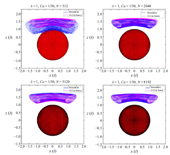
velocity field. Owing to the additional resolution needed to obtain converged streamlines, a detailed validation of our simulations is included in the Supplemental material. In § 3.4, we briefly present the
 $C \kern-1pt{-}\kern-1pt E$
plane representations of streamlines, with both inertia and drop deformation included, as a function of
 $Re/Ca$
. In § 4.1, we provide a summary of the main findings. We end with § 4.2, which provides a brief but broad overview of the expected relation between streamline topology and scalar transport, and thereby places the results of the present study in perspective; possible future extensions of the present effort are also mentioned. Appendices B.1 and B.2 discuss features pertaining to the averaged trajectories in the
 $C \kern-1pt{-}\kern-1pt E$
plane, in § 3.2, including numerical issues encountered in integrating the averaged equations in the vicinity of the Stokesian separatrix. Appendix C tabulates the
 $\lambda$
-dependent coefficients that appear in the expression for the
 $O(Ca)$
correction to the Stokesian velocity field.
2. Drop in canonical planar linear flows: streamline topology
An ambient planar linear flow is given by
 $\boldsymbol {u}^\infty = \boldsymbol {\Gamma } \cdot \boldsymbol {x}$
where
 \begin{align} \boldsymbol {\Gamma } = \begin{bmatrix} 0 & 2 & 0\\ 2\hat {\alpha } & 0 & 0\\ 0 & 0 & 0 \end{bmatrix}, \end{align}
is the transpose of the velocity gradient tensor, the parameter
 $\hat {\alpha }$
being a measure of the strength of vorticity relative to extension; as mentioned in the introduction, it ranges from
 $-1$
(solid-body rotation) to
 $1$
(planar extension), with
 $\hat {\alpha } = 0$
corresponding to simple shear flow. In what follows, we briefly present the results of Powell (Reference Powell1983) and Krishnamurthy & Subramanian (Reference Krishnamurthy and Subramanian2018a
), pertaining to the streamline topology outside a spherical drop in an ambient hyperbolic planar linear flow (
 $0 \lt \hat {\alpha } \leqslant 1$
), including the limiting case of simple shear, to lay the groundwork for our analysis of the deformed-drop streamline topology in § 3. The restriction to hyperbolic linear flows is because all exterior streamlines are closed for spherical drops in elliptic linear flows (
 $-1 \leqslant \hat {\alpha } \lt 0$
) regardless of
 $\lambda$
, and therefore, rather trivially, all streamlines are expected to transform to spiralling ones on including irreversible effects arising from inertia or drop deformation. In contrast, the presence of a separatrix demarcating regions of closed and open exterior streamlines, for ambient hyperbolic linear flows (and simple shear), allows for non-trivial topological consequences.
The components of the Stokesian velocity field for a spherical drop in an ambient planar linear flow, in a spherical coordinate system with polar axis aligned with the ambient vorticity, are given by (Powell Reference Powell1983)
 \begin{align} &u_r = (1 + \hat {\alpha }) r (A r^2 + B) \sin ^2 \theta \sin 2\phi , \end{align}
 \begin{align} &\qquad u_\theta = \frac {(1 + \hat {\alpha })}{2} r B \sin 2 \theta \sin 2 \phi , \end{align}
 \begin{align} &\quad u_{\phi } = (1 + \hat {\alpha })r \sin \theta (B \cos 2\phi - \beta ), \end{align}
where
 $\beta = (1 - \hat {\alpha })/(1 + \hat {\alpha })$
, and
 \begin{align} &\qquad B = 1 - \frac {\lambda }{(1 + \lambda )r^5}, \end{align}
 \begin{align} &A = \frac {5 \lambda }{2(1+\lambda )r^7} - \frac {5 \lambda + 2}{2(1+\lambda )r^5}, \end{align}
outside the drop (
 $r \geqslant 1$
). The streamline pattern associated with (2.2)–(2.4) is a function of
 $\hat {\alpha }$
and
 $\lambda$
, and that for
 $\hat {\alpha } = 0.25, \lambda = 10$
is shown in figure 1. From figure 1(a), which shows the streamlines in the
 $x_1 x_2$
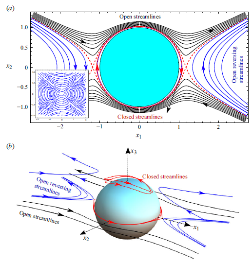
-plane, and figure 1(b), which depicts the full three-dimensional streamline pattern, the pattern is seen to consist of both open and closed streamlines, demarcated by a separatrix whose projection is shown as a dashed red curve. Mirroring the ambient flow (figure 1a
, inset), the open streamlines are themselves of two kinds: those that directly head from upstream to downstream infinity, and those that reverse direction in doing so. As will be evident from the arguments below, the closed streamline region around the drop in figure 1 arises because the
 $\lambda$
value is greater than an
 $\hat {\alpha }$
-dependent threshold.
Stokesian streamlines around a spherical drop for
 $\hat {\alpha } = 0.25,\,\lambda = 10$
: (a) the in-plane streamline pattern (inset shows the ambient streamlines for
 $\hat {\alpha } = 0.25$
); (b) the complete three-dimensional streamline topology; closed streamlines are shown in red, open streamlines in black, open-reversing streamlines in blue and the in-plane separatrix as a pair of dashed red curves. The closed-streamline region for this
 $\hat {\alpha }$
is finite in extent.

Towards characterizing the streamlines analytically, one may integrate (2.2)–(2.4) to obtain
 \begin{align} &x_2 = \pm r \left [ \frac {\hat {\alpha }}{(1 + \hat {\alpha })} + E f^2(r) + \frac {\beta \lambda }{1 + \lambda } f^2(r) g(r)\right ]^{1/2}, \end{align}
 \begin{align} &\qquad\qquad\qquad\qquad x_3 = r C f(r), \end{align}
where
 $f(r) = [ r^3 + ({(3 \lambda)}/{(2 (1 + \lambda ) r^2)}) - (({5\lambda + 2})/{(2(1 + \lambda ))}) ]^{-1/3}$
and
 $g(r) = \int _r^{\infty } ({f(y)}/{y^3}) {\rm d}y$
. Each of the streamlines in figure 1 may then be regarded as the curve of intersection of a pair of invariant surfaces belonging to the families (2.7) and (2.8), which are characterized by the parameters
 $C$
and
 $E$
(Cox et al. Reference Cox, Zia and Mason1968; Powell Reference Powell1983; Krishnamurthy & Subramanian Reference Krishnamurthy and Subramanian2018a
). A given streamline, either open or closed, corresponds therefore to an ordered pair
 $(C,E)$
.
From (2.7) and (2.8), the constant-
 $C$
and
 $E$
surfaces are seen to be surfaces of revolution about the
 $x_3$
and
 $x_2$
axes, respectively. Since
 $f(r) \rightarrow \infty$
for
 $r \rightarrow 1$
and
 $f(r) \rightarrow 0$
for
 $r \rightarrow \infty$
, the exterior fluid domain corresponds to
 $C \in [0,\infty )$
with the drop surface, together with the flow-gradient (
 $x_1x_2$
) plane, corresponding to the limiting surface
 $C = 0$
(owing to symmetry about the plane
 $x_3 = 0$
, we only consider half the domain corresponding to
 $x_3 \gt 0$
; identical results hold for the other half with the sign of
 $C$
reversed). The aforementioned limiting values of
 $f$
also imply
 $E\in [E_0,\infty )$
for the exterior fluid domain, with the drop alone corresponding to the inner limiting surface
 $E = E_0 = (-{\beta \lambda g(1)})/({1+\lambda })$
. Further,
 $E = E_{sep}$
is the axisymmetric separatrix surface that separates regions of closed (
 $E_0 \lt E \lt E_{sep}$
) and open (
 $E \gt E_{sep}$
) streamlines, and whose projection appears in figure 1(a). This surface intersects the
 $x_1 x_3$
-plane in a circle of degenerate fixed (saddle) points defined by
 $(r,\theta ,\phi ) \equiv [r_{sep}, \theta , (0,\pi )]$
with
 $r_{sep} = [({\lambda (1 + \hat {\alpha }))}/({2\hat {\alpha }(1+\lambda )})]^{{1}/{5}}$
; using this value of
 $r_{sep}$
in (2.8) leads to
 $E_{sep} = \frac {-\hat {\alpha }}{(1+\hat {\alpha })f^2(r_{sep})} - \frac {\beta \lambda }{(1+\lambda )}g(r_{sep})$
. Note that
 $r_{sep}$
diverges (and
 $E_{sep} \rightarrow 0$
) for simple shear flow, so that the separatrix surface extends out to infinity along the
 $x_1x_3$
-plane for this case, independent of
 $\lambda$
.
While almost every streamline corresponds to a
 $(C,E)$
pair as already mentioned, the exceptions are those on the drop surface which remain inaccessible owing to the two families of surfaces becoming tangential for
 $r \rightarrow 1$
; this is evident from the drop being a limiting member of both families (
 $C= 0$
or
 $E = E_0$
). Points along the
 $x_3$
-axis correspond trivially to zero-velocity streamlines for all
 $\hat {\alpha }$
and
 $\lambda$
, and arise as the points of tangency of the surfaces
 $C = 1/f(x_3)$
and
 $E = {-\hat {\alpha }/}{((1+\hat {\alpha })f^2(x_3))} - ({(\beta \lambda)}/{((1+\lambda )})g(x_3)$
; the other zero-velocity streamlines correspond to the points of intersection of the separatrix surface and the
 $x_1x_3$
-plane – this is the fixed-point circle referred to above. To characterize the nature of the non-degenerate streamlines for general
 $C$
and
 $E$
in more detail, we first consider the case
 $C = 0$
, corresponding to streamlines in the
 $x_1x_2$
-plane; features of the streamlines outside this plane may be inferred from the axisymmetry of the constant-
 $E$
surfaces. With
 $C = x_3 = 0$
, one has
 $0 \leqslant |x_2| \leqslant r$
, which leads to the following constraints on
 $E$
:
 \begin{align} \underbrace {\frac {-\hat {\alpha }}{f^2(r)(\hat {\alpha } + 1)} - \frac {\beta \lambda g(r)}{1 + \lambda }} &\leqslant \,&E\, \leqslant \underbrace {\frac {1}{f^2(r)(\hat {\alpha } + 1)} - \frac {\beta \lambda g(r)}{1 + \lambda }}. \\ F_2 (r;\hat {\alpha }, \lambda ) & & F_1 (r, \hat {\alpha }, \lambda ) \nonumber \end{align}
(a) The functions
 $F_1(r)$
(red) and
 $F_2(r)$
(blue) versus
 $r$
for
 $\hat {\alpha }=0.25,\,\lambda =10$
with
 $C = 0$
. The dashed red line with
 $E = E_{sep}$
corresponds to the in-plane separatrix, and demarcates open (maroon region) and closed (grey region) streamline regions. The solid orange line with
 $E = E_0$
separates the
 $E$
-interval corresponding to both closed and open reversing streamlines (
 $E_0 \lt E \lt E_{sep})$
, from the one corresponding to only the latter (
 $E\lt E_0$
) (blue region). Streamlines for three different
 $E$
values appear as horizontal segments; (b) the different classes of streamlines in the
 $x_1x_2$
-plane, corresponding to the horizontal segments/lines in (a). A given streamline is depicted in both the
 $F_1/F_2 \kern-1pt{-}\kern-1pt r$
and
 $x_1x_2$
planes using the same colour: green for
 $E\gt E_{sep}$
; black for
 $E_0\lt E\lt E_{sep}$
; violet for
 $E\lt E_0$
.

The nature of the in-plane streamlines can now be understood based on the behaviour of the functions
 $F_1$
and
 $F_2$
, which are plotted against
 $r$
in figure 2(a), for
 $\hat {\alpha } = 0.25,\;\lambda = 10$
– the parameter values in figure 1. In corresponding to a constant
 $E$
, and in light of (2.9), the in-plane streamlines must appear in figure 2(a), either as horizontal segments bounded between the
 $F_1$
and
 $F_2$
curves, or as horizontal lines that extend to infinity starting from either of these curves. For the chosen
 $\hat {\alpha }$
and
 $\lambda$
,
 $F_1$
is a strictly increasing function that starts from its minimum value of
 $E_0$
at
 $r = 1$
. While
 $F_2$
starts from the same point, it is non-monotonic, attaining a maximum value of
 $E_{sep}$
at
 $r = r_{sep}$
. The different classes of streamlines may now be organized as follows. Those with
 $E \gt E_{sep}$
have a finite
 $r_{min}\,(= F_1^{-1}(E)$
), but have
 $r_{max} = \infty$
, and are open streamlines running from upstream to downstream infinity in the same sense as the streamlines of the ambient flow; for a given
 $E$
(
 $= E_1$
in figure 2a
), there are two such streamlines (the green curves in figure 2b
), with one obtained from the other via a reflection about the
 $x_1$
-axis. There are two horizontal segments corresponding to each
 $E$
in the interval
 $E_0 \leqslant E \lt E_{sep}$
– the black segments with
 $E = E_2$
in figure 2(a): (i) the first is bounded between the
 $F_1$
and
 $F_2$
curves, with both
 $r_{min}\,(= F_1^{-1}(E))$
and
 $r_{max}\,(= F_2^{-1}(E))$
being finite, and therefore, corresponds to a closed streamline (the black closed curve in figure 2b
); (ii) the second starts from the
 $F_2$
-curve, extending out to infinity, with
 $r_{min}\,(=F_2^{-1}(E))$
finite and
 $r_{max} = \infty$
, and corresponds to a pair of open reversing streamlines (the open black curves on either side of the drop in figure 2b
). The marginal value,
 $E = E_{sep}$
, corresponds to the in-plane projection of the axisymmetric separatrix surface mentioned above, and consists of both closed and open (reversing) portions intersecting in a pair of saddle points given by
 $(x_1,x_2,x_3) \equiv (\pm r_{sep},0,0)$
; the separatrix projection appears as a dashed red curve in figure 2(b) (the same curve was seen in figure 1a
). As
 $E$
decreases below
 $E_{sep}$
, the closed streamline moves towards the drop while the pair of open reversing streamlines move away, until at
 $E = E_0$
, the former coincides with the drop surface. For
 $E \lt E_0$
, one only has open reversing streamlines (
 $E= E_3$
in figure 2a
); the purple curves in figure 2(b) that move off to infinity, along the positive and negative
 $x_1$
-directions, as
 $E \rightarrow -\infty$
. For the chosen
 $\hat {\alpha }$
and
 $\lambda$
, the region of closed streamlines in figure 2 is evidently finite in extent. For
 $\hat {\alpha } = 0$
,
 $r_{sep} = \infty \,\forall \,\lambda$
and
 $F_2(r)$
becomes a monotonically increasing function, asymptoting to a maximum (
 $E_{sep} =0$
) for
 $r \rightarrow \infty$
. Thus, for simple shear flow, the interval
 $E_0 \lt E \lt E_{sep}\,(= 0)$
corresponds only to closed streamlines, with the minimum,
 $E_0 =-({\lambda g(1)})/({1+\lambda})$
, corresponding to the drop surface.
Figure 3(a) plots
 $F_1$
and
 $F_2$
for the same
 $\hat {\alpha }\,(= 0.25)$
as in figure 2, but for
 $\lambda$
varying from
 $10$
down to
 $0.5$
. With decreasing
 $\lambda$
,
 $F_2$
transitions from a non-monotonic to a strictly decreasing function of
 $r$
with a maximum at
 $r = 1$
. The transition occurs across a threshold
 $\lambda = \lambda _c$
, which may be obtained by setting
 $r_{sep} = 1$
, giving
 $\lambda _c = ({2 \hat {\alpha }})/({1- \hat {\alpha }})$
;
 $\lambda _c = 2/3$
for
 $\hat {\alpha } = 0.25$
, so
 $\lambda \gt \lambda _c$
in figure 1. At
 $\lambda = \lambda _c$
,
 $F_2$
is seen to have a zero slope at the origin. Although not shown, an analogous transition occurs for
 $\lambda$
fixed, and for
 $\hat {\alpha }$
increasing beyond the threshold
 $\hat {\alpha }_c = \frac {\lambda }{2 + \lambda }$
. With
 $F_1$
monotonically increasing and
 $F_2$
monotonically decreasing, all streamlines in figure 3(a) are horizontal lines starting from either of these curves and extending to infinity, and hence, are open. Thus, the aforementioned threshold viscosity ratio corresponds to a critical curve in the
 $\hat {\alpha } - \lambda$
plane, separating in-plane streamline patterns that include a closed-streamline region in the vicinity of the spherical drop (as in figure 1), from those that do not. For
 $\hat {\alpha } = 1$
,
 $\lambda _c = \infty$
, and therefore, as mentioned in § 1, all in-plane streamlines remain open in planar extension regardless of
 $\lambda$
. At the other extreme,
 $\lambda _c = 0$
for
 $\hat {\alpha } = 0$
, so that a closed streamline region exists for all finite
 $\lambda$
in simple shear flow, being bounded by a separatrix curve that extends to infinity along the flow direction. This curve is in turn the projection of an axisymmetric separatrix surface that extends to infinity as it approaches the flow-vorticity plane, and includes an infinite volume of fluid within.
(a) The functions
 $F_1(r)$
(red) and
 $F_2(r)$
(blue) for
 $\hat {\alpha } = 0.25$
,
 $C = 0$
, for different
 $\lambda$
; (b) the functions
 $F_1(r)$
(red) and
 $F_2(r)$
(blue) for
 $\hat {\alpha } = 0.25$
,
 $\lambda = 10$
for varying
 $C$
. The magenta stars denote the intersection points of
 $F_1$
and
 $F_2$
, which move towards the right with increasing
 $C$
.

For
 $C \neq 0$
, the modified constraint
 $0 \leqslant |x_2| \leqslant \sqrt {r^2 - x_3^2}$
leads to the same expression for
 $F_2$
as in (2.9), but with
 $F_1 (r, \hat {\alpha }, \lambda ) = {1}/{(f(r)^2(\hat {\alpha } + 1))} - {(\beta \lambda g(r))}/{(1 + \lambda)} - C^2$
. Thus, the
 $F_1$
-curve is displaced downward by a constant amount. As shown in figure 3(b), for
 $\hat {\alpha } = 0.25$
and
 $\lambda = 10$
, with increasing
 $C$
, this displacement causes it to move across the maximum of the
 $F_2$
-curve (which remains unchanged) to larger
 $r$
, leading to the disappearance of the closed streamline region. Consistent with axisymmetry of the separatrix surface, this crossover to an open-streamline topology happens at
 $x_3 = r_{sep}$
, with
 $C=f(r_{sep})$
. Note again that
 $r_{sep} = \infty$
for simple shear flow, so the crossover does not happen at a finite
 $C$
, consistent with the infinite extent of the separatrix surface already mentioned.
The in-plane streamline pattern for a spherical drop in simple shear flow (
 $\hat {\alpha } = 0$
) with
 $\lambda = 10$
; closed streamlines are shown in red, open streamlines in black and the in-plane separatrix as a pair of dashed red curves. The closed-streamline region is now infinite in extent within the flow-vorticity plane, and there are no open-reversing streamlines.

The streamline patterns in figures 1(a) and 1(b) are readily interpreted based on the discussion above. Figure 4 shows the in-plane streamline pattern for
 $\hat {\alpha } = 0$
, again for
 $\lambda = 10$
; consistent with the above arguments, the region of closed in-plane streamlines is infinite in extent along the
 $x_1$
-axis, with there being no open reversing streamlines. We now discuss the compact representation of the spherical-drop-streamlines as points in the
 $C \kern-1pt{-}\kern-1pt E$
plane. Such a representation may be used to gainfully interpret the altered streamline topology in the presence of inertia (Subramanian & Koch Reference Subramanian and Koch2006a
,Reference Subramanian and Kochb
; Krishnamurthy & Subramanian Reference Krishnamurthy and Subramanian2018a
,Reference Krishnamurthy and Subramanianb
; appendix A), drop deformation (§ 3), suspending fluid viscoelasticity (Subramanian & Koch Reference Subramanian and Koch2007), etc. As is known from earlier rheological and transport rate calculations, the consequences of the altered streamline topology are most important in the region of closed streamlines, and therefore, we identify this region on the
 $C \kern-1pt{-}\kern-1pt E$
plane. This requires determining the
 $E$
-interval, corresponding to closed streamlines, as a function of
 $C$
. For
 $C = 0$
, as evident from figure 2(a),
 $E \in [E_0,E_{sep}]$
, with
 $E_0$
being the point of intersection of
 $F_1$
and
 $F_2$
that also corresponds to the smallest
 $r\,(=1)$
. For non-zero
 $C$
, the point of intersection moves to larger
 $r(\gt 1)$
, as shown in figure 3(b), and may be determined by solving
 $F_1(r) = F_2(r)$
– closed streamlines exist only for
 $r$
values greater than that corresponding to this point of intersection, and until
 $r = r_{sep}$
. One obtains the corresponding
 $E$
(
 $E_{min}(C)$
, say;
 $E_0 = E_{min}(0)$
) using (2.9), and the
 $E$
-interval therefore is
 $[E_{min}(C),E_{sep}]$
. This interval decreases with increasing
 $C$
, vanishing at
 $C = C^*$
(say) when
 $E_{min}(C^*) = E_{sep}$
. Here
 $C^*$
is finite for non-zero
 $\hat {\alpha }$
, diverging to infinity for
 $\hat {\alpha } \rightarrow 0$
. The region of closed streamlines in the
 $C \kern-1pt{-}\kern-1pt E$
plane is shown in grey in figures 5(a) and 5(b) for a pair of
 $(\hat {\alpha },\lambda )$
combinations. As evident from figure 2(a), open-reversing streamlines also exist over the same
 $E$
-interval for
 $\hat {\alpha } \neq 0$
, and the grey regions in the said figures therefore correspond to both closed and open-reversing streamlines. Each of these regions is bounded by the interval
 $[0,C^*]$
on the
 $C$
-axis, the interval
 $[E_0,E_{sep}]$
on the
 $E$
-axis, and the curve
 $E_{min}(C)$
. Almost all points on
 $E_{min}(C)$
correspond to minimal closed streamlines that are the points of tangency of the two surfaces involved. Only the point
 $(0,E_0)$
, at which the
 $E$
-axis and
 $E_{min}(C)$
meet, corresponds to the entire drop surface (
 $r=1$
); this abrupt transition from a point to a surface occurs on account of the coincidence of the surfaces
 $E= E_0$
and
 $C=0$
, as mentioned earlier. Although not of concern here, figures 5(a) and 5(b) also depict the adjoining regions (in cyan and maroon) consisting solely of open reversing and open streamlines, respectively; note that these regions do not exist for
 $\hat {\alpha } = 0$
, in which case the grey region corresponds solely to closed streamlines.
The
 $C \kern-1pt{-}\kern-1pt E$
planes for (a)
 $\hat {\alpha } = 10^{-3}, \lambda = 1\,(\gt \lambda _c)$
and (b)
 $\hat {\alpha } = 0.25, \lambda = 10\,(\gt \lambda _c)$
, showing the various streamline topologies and their regions of occurrence. Grey regions correspond to both closed and open reversing streamlines, while cyan regions correspond to open-reversing streamlines alone.

3. A weakly deformed drop in a hyperbolic planar linear flow
In this section, we analyse the streamline topology outside a weakly deformed drop in ambient planar hyperbolic flows, including the important limiting case of simple shear flow. As already mentioned in the introduction, drop deformation leads to interfacial forces that drive the drop towards sphericity even if the ambient shear were to be reversed. Therefore, drop deformation evidently breaks Stokesian reversibility, and similar to inertia, one expects an altered streamline topology for non-zero
 $Ca$
. We shall restrict ourselves to illustrating this alteration for
 $Ca \ll 1$
,
 $\lambda \sim O(1)$
, and will only briefly discuss the case of large viscosity (
 $\lambda \gg 1$
,
 $\lambda Ca \sim O(1)$
) in the conclusions. While the discussion of the streamline topology below is largely based on the
 $O(Ca)$
velocity field, in light of our findings contradicting the earlier efforts of Torza et al. (Reference Torza, Henry, Cox and Mason1971), Kennedy & Pozrikidis (Reference Kennedy and Pozrikidis1994) and Komrakova et al. (Reference Komrakova, Shardt, Eskin and Derksen2014), we also present the results of boundary element simulations which agree well with analytical predictions. The exterior velocity field, to
 $O(Ca)$
, is given by
 \begin{align} \boldsymbol {u} = \boldsymbol {u}^{(0)}(\boldsymbol {x}) + Ca\, \boldsymbol {u}^{(1)}(\boldsymbol {x}) + O(Ca^2), \end{align}
where
 $\boldsymbol {u}^{(0)}$
is given by (2.2)–(2.4), and
 $\boldsymbol {u}^{(1)}$
is given by (Greco Reference Greco2002)
 \begin{align} \begin{split} \boldsymbol {u}^{(1)} = &\,c_1(r,\lambda ) (\boldsymbol {E:}\boldsymbol {x}\boldsymbol {x})^2 \boldsymbol {x} + c_2(r) (\boldsymbol {E:}\boldsymbol {x}\boldsymbol {x}) \boldsymbol {E.}\boldsymbol {x} + c_3(r,\lambda ) (\boldsymbol {E:E})\boldsymbol {x} \\ & + c_4(r,\lambda ) (\boldsymbol {E.E:}\boldsymbol {x}\boldsymbol {x})\boldsymbol {x} + c_5(r,\lambda ) \boldsymbol {E.E.}\boldsymbol {x} + c_6(r,\lambda ) (\boldsymbol {A}_2\boldsymbol {:x}\boldsymbol {x})\boldsymbol {x} \\ & + c_7(r,\lambda ) \boldsymbol {A}_2\boldsymbol {.x}, \end{split} \end{align}
with
 $\boldsymbol {A}_2 = 2(\boldsymbol {E} \cdot \boldsymbol {\Omega } - \boldsymbol {\Omega } \cdot \boldsymbol {E}) + 4\boldsymbol {E} \cdot \boldsymbol {E}$
being the second Rivlin–Ericksen tensor; the
 $c_i(r,\lambda )$
values are defined in Appendix C. Note that (3.2) has essentially the same tensorial form as the
 $O(R{\kern-1pt}e)$
inertial correction in Appendix A (see (A2)), as must be the case since both expressions have a regular character, being quadratic functionals of the ambient velocity gradient. Unlike the inertial correction, (3.2) does satisfy the far-field decay requirement, and therefore (3.1) remains valid everywhere in the exterior domain for sufficiently small
 $Ca$
.
3.1. Exterior streamlines in physical space
Exterior streamlines around a deformed drop for
 $Ca = 0.0333\,(1/30), \lambda = 1$
(
 $\hat {\alpha }_c = 1/3$
): (a) and (b) correspond to
 $\hat {\alpha } = 0$
; (c) and (d) to
 $\hat {\alpha } = 10^{-2}$
; (e) and (f) to
 $\hat {\alpha } = 0.5\,(\gt \hat {\alpha }_c)$
. Panels (a), (c) and (e) show the three-dimensional streamlines; (b), (d) and (f) show those in the
 $x_1 \kern-1pt{-}\kern-1pt x_2$
plane. The magenta points mark the ‘initial’ points from which one carries out forward and backward integrations in time.

We now characterize the finite-
 $Ca$
streamline topology arising from (3.1), by fixing a
 $\lambda$
and plotting the streamlines for various
 $\hat {\alpha }$
. Thus, in figure 6(a–f), we have chosen
 $\lambda = 1$
,
 $Ca = 0.0333$
, and have plotted the exterior streamlines for
 $\hat {\alpha } = 0$
(figures 6a
and 6b
),
 $10^{-2}$
(figures 6
c and 6
d) and
 $0.5$
(figures 6
e and 6
f); the final
 $\hat {\alpha }$
is greater than
 $\hat {\alpha }_c\,(=1/3)$
, so there is no zero-
 $Ca$
closed-streamline region in this case. From figures 6(a) and 6(c), the streamlines are seen to come in from infinity towards the drop surface along an intermediate direction, and then spiral out along the
 $x_3$
-axis (the blue streamlines), or spiral outward as they approach the
 $x_1x_2$
-plane (the orange streamlines); the latter being consistent with the direction of spiralling within this plane, shown in figures 6(b) and 6(d). The zero-
 $Ca$
separatrix surface organizes the finite-
 $Ca$
streamlines into three groups: (i) fore–aft asymmetric (about the
 $x_2$
-axis) open streamlines that go from upstream to downstream infinity in the same sense as the ambient ones; (ii) streamlines that spiral around the drop, heading out either along the
 $x_3$
axis, or outwards sufficiently close to the
 $x_1x_2$
-plane (they resemble the time-reversed versions of the inertial spiralling streamlines in the bifurcated-wake regime; see figure 2 in the Supplementary material); and (iii) for
 $\hat {\alpha } \neq 0$
, with a zero-
 $Ca$
Stokesian separatrix that is finite in extent in the
 $x_1x_3$
-plane, the spiralling streamlines above are contained between regions of fore–aft asymmetric (about the
 $x_1$
-axis) open reversing streamlines. Note that, for
 $\hat {\alpha } \gt \hat {\alpha }_c$
, the absence of a separatrix surface for
 $Ca = 0$
implies that all finite-
 $Ca$
streamlines fall into categories (i) and (iii), see figures 6(e) and 6(f).
While all streamlines that spiral outward, as they approach the
 $x_1x_2$
-plane, eventually head off to infinity, not all finite-
 $Ca$
streamlines, which spiral out along the
 $x_3$
-axis, go off to infinity. In fact, for
 $\hat {\alpha } = 0$
, integration for longer times shows, rather surprisingly, that every streamline that initially spirals out along the
 $x_3$
-axis turns around and come back towards the
 $x_1 \kern-1pt{-}\kern-1pt x_2$
plane. The streamline traces out a torus in the process, and eventually ends up winding densely on this invariant torus. This unexpected doubly periodic behaviour of a finite-
 $Ca$
streamline, with widely separated periods of
 $O(\dot {\gamma }^{-1})$
and
 $O(\dot {\gamma }^{-1}Ca^{-1})$
, is illustrated in figure 7 via plots of all three Cartesian coordinates as functions of time for
 $Ca = 0.0333$
and
 $Ca = 0.1$
. Next, figure 8(a) presents a three-dimensional view of a particular invariant torus for
 $\hat {\alpha } = 0$
; projections of this torus onto the principal Cartesian planes are shown in figure 8(b–d). The torus is seen to be highly distorted with its largest span in the
 $x_1 \kern-1pt{-}\kern-1pt x_3$
plane, and being far narrower in the other two planes. The nature of this distortion is the same for all invariant tori, and is consistent with the shape of the zero-
 $Ca$
separatrix surface for simple shear flow.
The Cartesian coordinates of finite-
 $Ca$
spiralling streamlines, which spiral out along the vorticity axis for
 $t \approx 0$
, plotted over times longer than
 $O(Ca^{-1}\dot {\gamma }^{-1})$
;
 $\hat {\alpha } = 0$
,
 $\lambda = 1$
, with
 $Ca = 0.0333$
(blue) and
 $Ca = 0.1$
(red). A short-time depiction of the streamline, for
 $Ca = 0.0333$
, appears (in blue) in figure 6(a). For both
 $Ca$
, the streamlines exhibit a quasiperiodic behaviour arising from dense winding around an invariant torus.

(a) Depiction of the dense winding of a finite-
 $Ca$
spiralling streamline (
 $Ca = 0.0333$
), around an invariant torus; this streamline was shown (in blue) earlier in figure 6(a), for shorter times, where it had started to spiral out along the
 $x_3$
-axis. Panels (b) to (d) show projections of the streamline onto the three Cartesian planes.

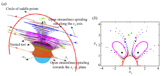
Figure 9(a) clarifies the global streamline topology for
 $\hat {\alpha } = 0, \lambda = 1$
and
 $Ca = 0.0333$
via the simultaneous depiction of multiple finite-
 $Ca$
streamlines, which helps highlight the configuration of nested invariant tori that arises for small but finite
 $Ca$
. The outermost torus extends to infinity in the
 $x_1\kern-1pt{-}\kern-1pt x_3$
plane, its spatial extent in this plane being indicated by the pair of dash–dotted lines (in green). In contrast, the innermost torus is a closed curve looping around the
 $x_3$
-axis, and is, in fact, one of the closed streamlines (perturbed by
 $O(Ca)$
) around the original undeformed drop. The projections of spiralling streamlines on the nested tori, generated via points of intersection of each streamline with the
 $x_1 \kern-1pt{-}\kern-1pt x_3$
plane, appear in figure 9(b). Since each of these streamlines winds indefinitely on an invariant torus, the points of intersection, taken over sufficiently many windings, densely fill out a closed curve in the said plane. Based on its projection, the outermost torus is seen to only occupy a fraction of the deformed drop surface (that appears as a red semicircle). The remainder of the drop is covered by streamlines that spiral in towards the drop on the outside of the outermost torus, and then along the drop surface towards the
 $x_1 \kern-1pt{-}\kern-1pt x_2$
plane, before moving off to infinity at a location closer to this plane. An example of such a streamline is the orange curve in figure 9(a), whose points of intersection with the
 $x_1 \kern-1pt{-}\kern-1pt x_3$
plane have been indicated (again in orange) in figure 9(b). In contrast to the densely winding streamlines above, the points of intersection are much more sparsely distributed on account of each such open streamline only spending a finite time in the neighbourhood of the drop.
(a) The exterior streamline topology for
 $\hat {\alpha } = 0$
,
 $\lambda = 1$
and
 $Ca = 0.0333$
: three of the tori, including the innermost singular curve (in black), which form part of the nested tori structure for non-zero
 $Ca$
, are highlighted; the orange streamline spirals in towards the drop from infinity, while remaining outside of the nested tori configuration, eventually escaping to infinity in the vicinity of the flow-gradient (
 $x_1 \kern-1pt{-}\kern-1pt x_2$
) plane. (b) Projections of the three invariant tori, and of open streamlines spiralling towards the flow-gradient plane, onto the flow-vorticity (
 $x_1 \kern-1pt{-}\kern-1pt x_3$
) plane. The projections have been generated by plotting the points of intersection of the finite-
 $Ca$
streamlines, with this plane; the projection of the drop appears as a red semicircle.

(a) The exterior streamline topology for
 $\hat {\alpha } = 10^{-4}$
,
 $\lambda = 1$
and
 $Ca = 0.0333$
; the finite separatrix surface intersects the
 $x_1 \kern-1pt{-}\kern-1pt x_3$
plane in the red circle shown. The pink streamline winds around on an invariant torus, with the black curve being a good approximation of the innermost singular torus. The remaining streamlines spiral in towards the drop surface, and then either towards the
 $x_1 \kern-1pt{-}\kern-1pt x_2$
-plane (orange curve), or out along the vorticity axis (green, brown and black curves). Panel (b) depicts the points of intersection of the curves in (a) with the
 $x_1 \kern-1pt{-}\kern-1pt x_3$
plane. Similar to figure 13(b), the tori only occupy a fraction of the drop surface.

The finite-
 $Ca$
streamline topology for a non-zero
 $\hat {\alpha }\,(=10^{-4})$
, again for
 $\lambda = 1$
,
 $Ca = 0.0333$
, is depicted in figure 10(a). The structure remains qualitatively similar to that for
 $\hat {\alpha } = 0$
, in that there still exists a configuration of nested invariant tori (the pink and black streamlines). However, the finite extent of the original zero-
 $Ca$
separatrix surface, and the saddle points at its rim (along a circle in the
 $x_1 \kern-1pt{-}\kern-1pt x_3$
plane), imply that the outermost torus is no longer infinite in extent. As a result, not all finite-
 $Ca$
streamlines, which begin spiralling outward along the
 $x_3$
-axis, turn back and continue to wind around invariant tori for all time. A subset of these streamlines, which start sufficiently close to the
 $x_3$
axis (this neighbourhood gets progressively smaller for decreasing
 $\hat {\alpha }$
, becoming vanishingly small for
 $\hat {\alpha } \rightarrow 0$
), approach the aforementioned fixed-point circle sufficiently closely, when starting to spiral back towards the
 $x_1 \kern-1pt{-}\kern-1pt x_2$
plane. This close approach causes the streamlines to exit the spiralling zone at some point, and head off to downstream infinity similar to an open streamline; the time-reversed version of this argument implies that such streamlines should also have come into the spiralling zone, from infinity, at a finite time in the past. The green, brown and blue streamlines in figures 10(a) and 10(b) exhibit this behaviour. Thus, there emerges a new class of streamlines (relative to those that exist for
 $\hat {\alpha } = 0$
) that appear to spiral around on an invariant torus, but eventually transform to open streamlines upon close approach to the saddle-point circle. Related to this is the emergence of a ‘gap’ between the outermost torus and the deformed drop surface, for non-zero
 $\hat {\alpha }$
, as highlighted via the nested-tori projections in figure 10(b). The existence of this gap implies that, unlike
 $\hat {\alpha } = 0$
, streamlines that come in from infinity, and reach the immediate vicinity of the drop surface, can now spiral out to infinity in one of two ways: either by spiralling towards the
 $x_1 \kern-1pt{-}\kern-1pt x_2$
plane, and then to downstream infinity, similar to
 $\hat {\alpha } = 0$
(the orange streamline in figure 10a
); or, by spiralling away from this plane, through the aforementioned gap, and then continuing to spiral on the outside of the nested-tori configuration, before escaping to infinity due to a close approach towards the fixed-point circle (the green, brown and blue streamlines mentioned above).
In summary, drop deformation does destroy the region of closed streamlines for any non-zero
 $Ca$
. The resulting finite-
 $Ca$
streamline topology appears more complex than its finite-
 $Re$
counterpart discussed in Appendix A. This complexity is highlighted by the existence of finite-
 $Ca$
streamlines that wind densely around a configuration of nested invariant tori, this configuration being embedded within a region of spiralling streamlines. The presence of such a structure is counter-intuitive, given its structural instability (in the sense of being susceptible to small perturbations) from the dynamical systems perspective. While the nature of individual finite-
 $C\!a$
streamlines is evident from figures 9 and 10, one can only afford to plot a few streamlines in each of these figures for purposes of clarity. With the intent of representing the whole streamline pattern, we move towards a compact representation of the finite-
 $C\!a$
streamlines on the
 $C \kern-1pt{-}\kern-1pt E$
plane.
3.2. The C − E representation of the exterior streamlines
There are two time scales associated with a tightly spiralling streamline for small
 $Ca$
: (i) the fast time scale of
 $O(\dot {\gamma }^{-1})$
characterizing the circulation around the closed Stokesian streamlines, and that is also the time in which the spiralling streamline executes a single turn; (ii) the asymptotically longer time scale of
 $O(\dot {\gamma }^{-1}Ca^{-1})$
in which the deformation-induced drift (across closed Stokesian streamlines) displaces a fluid element through a distance of
 $O(a)$
. While
 $C$
and
 $E$
were constants of motion in the Stokes limit, for small but finite
 $Ca$
, they vary on the aforementioned slow time scale. The equations governing this slow variation may be derived using the method of averaging (Bajer & Moffat Reference Bajer and Moffat1990). To do so, we start with the definitions in (2.7) and (2.8), rewritten as
 \begin{align} &\qquad\qquad\qquad\qquad\qquad C = \frac {\cos \theta }{f(r)}, \end{align}
 \begin{align} &E = \frac {1}{f^2(r)} \left (\sin ^2 \theta \sin ^2 \phi - \frac {\hat {\alpha }}{(1+\hat {\alpha })} - \frac {\beta \lambda }{1 + \lambda } f^2(r)g(r) \right ), \end{align}
where
 $x_2$
and
 $x_3$
have been replaced by their expressions in spherical coordinates. Differentiating (3.3) and (3.4) with respect to time, and using
 ${{\rm d}\boldsymbol {x}}/{{\rm d} t} = \boldsymbol {u}^{(0)}\boldsymbol {(x)} + Ca \; \boldsymbol {u}^{(1)}\boldsymbol {(x)}$
, one obtains
 \begin{align} \frac {{\rm d}C}{{\rm d}t} = \mathcal {F}_0(r,\theta ,\phi ) + Ca \; \mathcal {F}_1(r,\theta ,\phi ), \end{align}
 \begin{align} \frac {{\rm d}E}{{\rm d}t} = \mathcal {G}_0(r,\theta ,\phi ) + Ca \; \mathcal {G}_1(r,\theta ,\phi ), \end{align}
where
 \begin{align} &\mathcal {F}_0(r,\theta ,\phi ) = \frac {1}{f^2(r)} \left ( \sin \theta f(r) u_{\theta }^{(0)} + \cos \theta f'(r) u_{r}^{(0)} \right ), \end{align}
 \begin{align} &\mathcal {F}_1(r,\theta ,\phi ) = \frac {1}{f^2(r)} \left (\sin \theta f(r) u_{\theta }^{(1)} + \cos \theta f'(r) u_{r}^{(1)} \right ), \end{align}
 \begin{align} &\qquad\qquad\mathcal {G}_0(r,\theta ,\phi ) = u_\theta ^{(0)} I_1 + u_r^{(0)} I_2 + u_\phi ^{(0)} I_3, \end{align}
 \begin{align} &\qquad\qquad\mathcal {G}_1(r,\theta ,\phi ) = u_\theta ^{(1)} I_1 + u_r^{(1)} I_2 + u_\phi ^{(1)} I_3, \end{align}
with
 $I_{1} = f^2(r) \sin ^{2}\phi \sin 2 \theta$
,
 $I_{2} = 2 f(r) f'(r) ({\hat {\alpha }}/{(1 \!+ \hat {\alpha})}\! - \sin ^{2}\phi \sin ^{2}\theta ) \!+\! ({(\beta \lambda f^5(r))}/ {((1 + \lambda ) r^{3})})$
and
 $I_{3} = f^{2}(r) \sin ^{2}\theta \sin 2 \phi$
. On using (2.2)–(2.4) for
 $u_l^{(0)}$
(
 $l \equiv r, \theta , \phi$
),
 $\mathcal {F}_0$
and
 $\mathcal {G}_0$
, turn out to be identically zero, consistent with
 $C$
and
 $E$
being invariants of the Stokesian field. Equations (3.5) and (3.6) therefore reduce to
 \begin{align} \frac {{\rm d} C}{{\rm d}t} = Ca \; \mathcal {F}_1(r,\theta ,\phi ), \end{align}
 \begin{align} \frac {{\rm d}E}{{\rm d}t} = Ca \; \mathcal {G}_1(r,\theta ,\phi ), \end{align}
where the expressions for
 $u_l^{(1)}$
, involved in the definitions of
 $\mathcal {F}_1$
and
 $\mathcal {G}_1$
, are given by (3.2). Combining
 $Ca$
with
 $t$
on the left-hand side to give
 $\hat {t} = Ca \; t$
, the slow time variable in the method of averaging framework, and regarding
 $C$
and
 $E$
as being functions of
 $\hat {t}$
alone, at leading order in
 $Ca$
, (3.13) and (3.14) may be written in the form
 \begin{align} \frac {{\rm d} C}{{\rm d}\hat {t}} = \mathcal {F}_1[r(t;C,E),\theta (t;C,E),\phi (t;C,E)], \end{align}
 \begin{align} \frac {{\rm d}E}{{\rm d}\hat {t}} = \mathcal {G}_1[r(t;C,E),\theta (t;C,E),\phi (t;C,E)]. \end{align}
The right-hand side now explicitly recognizes that
 $r$
,
 $\theta$
and
 $\phi$
also depend on the fast time variable,
 $t$
, with this dependence arising, at leading order, from motion (approximately) along a Stokesian streamline corresponding to a given
 $C$
and
 $E$
. One obtains the averaged equations by integrating both sides of (3.13) and (3.14) over a single fast time period,
 \begin{align} \frac {{\rm d} C}{{\rm d}\hat {t}} = \bar {\mathcal {F}_1}(C,E) \; = \; \frac {1}{t_{period}} \int _0^{t_{period}} \mathcal {F}_1 \; {\rm d}t, \end{align}
 \begin{align} \frac {{\rm d}E}{{\rm d}\hat {t}} = \bar {\mathcal {G}_1}(C,E) \;= \; \frac {1}{t_{period}} \int _0^{t_{period}} \mathcal {G}_1 \; {\rm d}t, \end{align}
where the left-hand side of (3.15) and (3.16) are unaffected by the averaging since
 $C$
and
 $E$
are independent of
 $t$
. The fast-time integration above corresponds to a fixed
 $\hat {t}$
, and hence, to fixed
 $C$
and
 $E$
at leading order, with
 $t_{period}$
being the period of circulation around a given Stokesian streamline
 $(C,E)$
. One may therefore write
 \begin{align} \begin{split} &t_{period}(C,E) = 4 \int _{r_{min}(C,E)}^{r_{max}(C,E)} (u_r^{(0)})^{-1} {\rm d}r, \\ &\quad= 4 \int _{r_{min}(C,E)}^{r_{max}(C,E)} \frac {r^2 f(r) \; {\rm d}r}{\left [ \frac {\hat {\alpha }}{(1 + \hat {\alpha })f(r)^2} + \beta \left ( E + \frac {\beta \lambda }{1 + \lambda } g(r) \right ) - f^2(r) \left (E + \frac {\beta \lambda }{1 + \lambda } g(r) \right )^2 \right ]^{1/2}}, \end{split} \end{align}
where the four-fold symmetry of the Stokesian closed streamlines is used in converting the time integration to one over the radial coordinate; this also implies that the
 $\theta$
and
 $\phi$
in the integrands of (3.15) and (3.16) are now expressed in terms of
 $r$
using (3.3) and (3.4). The integration limits in (3.17) correspond to the minimum and maximum radial distances of the Stokesian streamline which always occur at
 $\phi = \frac {\pi }{2}$
and
 $\phi = 0$
, respectively, leading to the following relations for
 $r_{min}$
and
 $r_{max}$
:
 \begin{align} &\left [ \frac {\hat {\alpha }}{(1 + \hat {\alpha })} + E f^2(r_{min}) + \frac {\beta \lambda }{1 + \lambda } f^2(r_{min}) g(r_{min})\right ] = 1 - C^2 f^2(r_{min}), \end{align}
 \begin{align} &\qquad\quad\left [ \frac {\hat {\alpha }}{(1 + \hat {\alpha })} + E f^2(r_{max}) + \frac {\beta \lambda }{1 + \lambda } f^2(r_{max}) g(r_{max})\right ] = 0, \\[6pt] \nonumber \end{align}
which are again derived from the definitions of
 $C$
and
 $E$
. Using all relevant expressions in (3.15) and (3.16), one finally obtains the following two-dimensional autonomous system in explicit form:
 \begin{align} &\frac {{\rm d}C}{{\rm d} \hat {t}} = -\frac {\int _{r_{min}}^{r_{max}} \left ( \sin \theta f(r) u_{\theta }^{(1)} + \cos \theta f'(r) u_{r}^{(1)} \right )f(r)^{-2} (u_r^{(0)})^{-1} {\rm d}r}{\int _{r_{min}}^{r_{max}} (u_r^{(0)})^{-1} {\rm d}r}, \end{align}
 \begin{align} &\qquad\quad\frac {{\rm d}E}{{\rm d} \hat {t}} = \frac {\int _{r_{min}}^{r_{max}} \left ( u_\theta ^{(1)} I_1 + u_r^{(1)} I_2 + u_\phi ^{(1)} I_3 \right ) (u_r^{(0)})^{-1} {\rm d}r}{\int _{r_{min}}^{r_{max}} (u_r^{(0)})^{-1} {\rm d}r}, \end{align}
whose solutions are
 $Ca$
-independent trajectories in the
 $C \kern-1pt{-}\kern-1pt E$
plane.
The above derivation only applies within the region of closed streamlines that exists for
 $Ca = 0$
. Drop deformation perturbs the open streamlines in a regular sense, leading to an
 $O(Ca)$
difference between the upstream and downstream branches of any open streamline; there is no notion of multiple time scales in this case. We therefore numerically integrate (3.20) and (3.21) only in the region of the
 $C \kern-1pt{-}\kern-1pt E$
plane corresponding to the Stokesian closed streamline region – these regions have already been depicted (in grey) in figures 5(a) and 5(b). The integration involves starting from a given
 $(C,E)$
within the said region, and then proceeding forward and backwards in time until one approaches any of the boundaries shown in figure 5 (
 $E = E_{min}(C)$
,
 $E=E_{sep}$
or
 $C =0$
); note that one has to solve the transcendental relations (3.18) and (3.19), for
 $r_{min}$
and
 $r_{max}$
, at each time step in this integration. When integrated in this manner, the averaged trajectories obtained from (3.20) and (3.21) remain confined to the closed-streamline region for all times, only asymptoting to
 $E = E_{sep}$
in the limit
 $\hat {t} \rightarrow \pm \infty$
. This is because the velocity of an averaged trajectory, (
 ${{\rm d}C}/{{\rm d}\hat {t}},{{\rm d}E}/{{\rm d}\hat {t}}$
), goes to zero for
 $E \rightarrow E_{sep}$
, owing to the divergence of the period of circulation in this limit; the nature of this divergence is analysed in more detail in Appendix B.1.
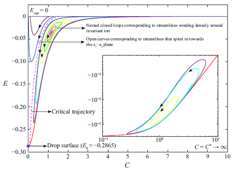
Figure 11 depicts the averaged trajectories on the
 $C \kern-1pt{-}\kern-1pt E$
plane for
 $\hat {\alpha } = 0, \lambda = 1$
. The zero-
 $C\!a$
closed-streamline region clearly consists of two distinct parts. The trajectories on the right-hand side form a system of nested closed curves which extends right up to the separatrix (
 $E_{sep} = 0$
) – see inset. These closed curves correspond to the configuration of nested invariant tori in figure 9. Note that each closed curve corresponds to the entire set of streamlines winding around a given torus. In contrast, the trajectories on the left are open; they start from the separatrix, extend downwards to lower
 $E$
and smaller
 $C$
, before turning around and proceeding in the direction of increasing
 $E$
, again ending up on the separatrix in the limit of infinite time. They resemble time-reversed versions of inertial trajectories, in the analogous region of the
 $C \kern-1pt{-}\kern-1pt E$
plane, for the bifurcated-wake regime (see figure 19b
in Appendix A). In figure 9, these trajectories correspond to open streamlines outside of the invariant tori, that spiral in towards the
 $x_1 \kern-1pt{-}\kern-1pt x_2$
plane, before going off to infinity. The dashed pink curve in figure 11 is an approximate depiction of the critical trajectory that demarcates the two classes of trajectories above, and extends from the separatrix to the drop surface (
 $E = E_0, C = 0$
). In fact, the outermost closed curve may be interpreted as a composite one, consisting of the aforementioned critical curve and the red curve
 $E_{min}(C)$
, connected at the terminal points – (
 $E = E_0, C = 0$
), corresponding to the drop, and (
 $E =E_{sep},C\rightarrow \infty$
), corresponding to the point at infinity on the separatrix surface. In physical space, this corresponds to the outermost torus being interpreted as a composite of the part of the separatrix surface whose projection (onto the
 $x_1 \kern-1pt{-}\kern-1pt x_3$
plane) is the pair of green dash–dotted lines in figure 9(b), the enclosed portion of the drop surface (with projection being the portion of the red curve between the pair of green lines), and the vorticity axis.
The
 $C \kern-1pt{-}\kern-1pt E$
plane representations of streamlines for small but finite
 $C\!a$
;
 $\hat {\alpha } = 0$
,
 $\lambda = 1\,(\gt \lambda _{c}= 1/3)$
. The dashed pink curve is an approximate depiction of the critical trajectory that separates open trajectories (streamlines spiralling towards the flow-gradient plane, and then to infinity) on the left, from a configuration of nested closed curves (streamlines that wind densely around nested invariant tori) on the right. The inset, on a log–log scale, shows that the nested closed-curve configuration extends right until the separatrix.

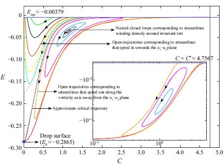
The
 $C \kern-1pt{-}\kern-1pt E$
plane representation, for small but finite
 $C\!a$
, for
 $\hat {\alpha } = 10^{-4}$
,
 $\lambda = 1\,(\gt \lambda _{c})$
. The nearly coincident dashed grey and violet curves are approximations (with differing resolutions,
 $N_G = 300$
and
 $2000$
) of the critical trajectory that demarcates two groups of streamlines: the first group consists of those that spiral towards the
 $x_1 \kern-1pt{-}\kern-1pt x_2$
plane and then to infinity); the second group includes those that wind densely around nested invariant tori, and those that spiral in towards the drop and then out to infinity along the
 $x_3$
-axis. The dashed grey (
 $N_G = 300$
) and cyan (
 $N_G =2000$
) curves correspond to differing-resolution depictions of an open trajectory in the neighbourhood of the critical trajectory.

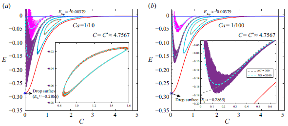
Figure 12 depicts the averaged trajectories for
 $\hat {\alpha } = 10^{-4}, \lambda = 1$
. Not all trajectories on the right-hand side of the critical curve (shown in dashed-grey and magenta for different resolutions) are now closed. While the closed trajectories still correspond to invariant tori in physical space, there are open trajectories running around the configuration of nested closed curves, and that start and end on the separatrix (
 $E_{sep} = -0.00379$
); an example being the orange curve shown both in the main plot and the inset. These correspond to the streamlines in figure 10 that spiral in towards the drop outside of the invariant tori, and then to infinity along the
 $x_3$
-axis. Unlike in figure 11, the outermost torus, corresponding to the largest closed curve, must now be finite in extent, and must separate the aforementioned groups of trajectories. Further, it must touch the separatrix at a finite
 $C$
, with finite-time uniqueness constraints implying that this point be singular (for instance, a corner). Our attempts at identifying the nature of this singular curve have, however, been frustrated by convergence difficulties in the vicinity of the separatrix, which are discussed in Appendix B.2. While trajectories on the left-hand side of the critical curve are still all open, and therefore must start and end on the separatrix similar to figure 11, convergence difficulties affect the ones immediately to the left-hand side of the said curve. For a given numerical resolution, there appears to be a (left-hand side) neighbourhood of the critical curve where trajectories, rather than turning around and heading up towards the separatrix, head down towards the drop instead. The neighbourhood shrinks with increasing resolution, as illustrated by the differing character of the dashed-grey (lower resolution) and cyan (higher resolution) curves in figure 12; note that `resolution’ here refers to the number of quadrature points (
 $N_G$
) used in evaluating the averaging integrals on the right-hand side of (3.20) and (3.21). This convergence difficulty is absent for the inertial case examined in Appendix A, and appears to be an artefact of drop deformation.
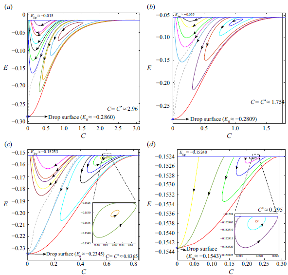
Figure 13(a–d) show the
 $C \kern-1pt{-}\kern-1pt E$
plane representations for larger
 $\hat {\alpha }$
, up until
 $\hat {\alpha } = 0.3$
which is just less than
 $\hat {\alpha }_c = \frac {1}{3}$
. Despite decreasing in size with increasing
 $\hat {\alpha }$
, the configuration of nested closed curves on the right appears to persist for
 $\hat {\alpha } \rightarrow \hat {\alpha }_c^-$
; this persistence being illustrated by the insets in figures 13(c) and 13(d). The reduction in size implies that a greater fraction of trajectories on the right-hand side are open ones that start (at a lower
 $C$
) and end (at a higher
 $C$
) on the separatrix. The drop-deformation-induced convergence artefact mentioned above leads to an increasing fraction of trajectories on the left-hand side heading towards the drop, instead of the separatrix (as opposed to only the critical curve). Again, however, an increase in resolution leads to improved representations – compare the coloured (higher resolution) trajectories in figure 13(a–c) with the corresponding dashed-grey (lower resolution) ones. For figure 13(d), even the higher-resolution trajectories on the left-hand side head towards the drop; the vicinity to
 $\hat {\alpha }_c$
seems to require a greater resolution in this case.
The
 $C \kern-1pt{-}\kern-1pt E$
plane representations for (a)
 $\hat {\alpha } = 10^{-3}$
, (b)
 $\hat {\alpha } = 10^{-2}$
, (c)
 $\hat {\alpha } = 10^{-1}$
and (d)
 $\hat {\alpha } = 0.3$
;
 $\lambda = 1$
,
 $\hat {\alpha }_c = \frac {1}{3}$
. A system of nested closed curves exists up until
 $\hat {\alpha } = \hat {\alpha }_c$
, as indicated by insets in (c) and (d); although, this system decreases in size for
 $\hat {\alpha } \rightarrow \hat {\alpha }_c$
, while also approaching the separatrix. The dashed grey curves in all panels correspond to lower-resolution trajectories (
 $N_G = 300$
) that (erroneously) head towards the drop, as opposed to the separatrix; increasing the resolution (to
 $N_G = 2000$
) restricts this error to an increasingly small neighbourhood of the critical curve.

In figure 14, we compare averaged trajectories with the corresponding full-solution trajectories, obtained from integration of the velocity field in (3.1), for
 $\hat {\alpha } = 10^{-4}, \lambda = 1$
. The full-solution trajectories have a two-time scale character with fast oscillations superposed on a slow drift, the latter being captured by the method of averaging at leading order. Notwithstanding the fast oscillations, the full-solution trajectories compare well with the averaged ones for both
 $C\!a = 0.1$
(figure 14a
) and
 $0.01$
(figure 14b
), over most of the
 $C \kern-1pt{-}\kern-1pt E$
plane; the amplitude of the oscillations being smaller for
 $C\!a = 0.01$
. Further, unlike the averaged trajectories, the full-solution trajectories on the left-hand side of the closed-streamline region do cross the separatrix, spiralling out to infinity close to the
 $x_1 \kern-1pt{-}\kern-1pt x_2$
plane. Once outside the closed-streamline region, the trajectories converge to a finite point above the separatrix because of the rapidity of decay, of the
 $O(C\!a)$
velocity field, at large distances; this is in contrast to the inertial trajectories analysed in Appendix A. Two more points are worth noting. First, for comparable
 $C\!a$
and
 $R{\kern-1pt}e$
, the full-solution trajectories in the former case exhibit much larger amplitudes of the fast wiggles – compare figures 20(a) and 14(b). This is indicative of the dominant role of drop deformation for similar magnitudes of
 $R{\kern-1pt}e$
and
 $C\!a$
, and this will be seen again in § 3.4 below where we examine the averaged trajectories as a function of
 $R{\kern-1pt}e/C\!a$
. Second, the full-solution trajectories respect the deformation of the drop. Thus, as emphasized via the inset in figure 14(b), these trajectories invariably turn around and cross the separatrix, despite the corresponding averaged trajectory (when close enough to the critical curve) heading towards the drop owing to insufficient numerical resolution (the dashed grey curves in figures 14a
and 14b
).
The
 $C \kern-1pt{-}\kern-1pt E$
plane for
 $\hat {\alpha } = 10^{-4}$
,
 $\lambda = 1$
. Trajectories from the averaging analysis are compared with the full-solution trajectories for (a)
 $C\!a = 0.1$
and (b)
 $C\!a = 0.01$
. Grey and blue dashed curves correspond to lower (
 $N_G = 300$
) and higher (
 $N_G= 2000$
) resolution averaged trajectories.

3.3. Boundary element simulations
The exterior streamline topology detailed in the earlier two subsections is non-trivial for two reasons. The first, as already mentioned in the introduction, is that our findings go against the belief prevailing in the literature (Torza et al. Reference Torza, Henry, Cox and Mason1971; Kennedy & Pozrikidis Reference Kennedy and Pozrikidis1994; Komrakova et al. Reference Komrakova, Shardt, Eskin and Derksen2014). The second is that, from a dynamical systems perspective, one expects the nested-tori configuration to be structurally unstable, and thereby susceptible to additional perturbations which include deformation-induced corrections of an order higher than the
 $O(Ca)$
correction examined in §§ 3.1 and 3.2. This latter reason motivated us to perform BEM simulations, following along the lines of Kennedy & Pozrikidis (Reference Kennedy and Pozrikidis1994) and Pozrikidis (Reference Pozrikidis2002). The BEM simulations have, of course, been extensively used in the earlier literature for the study of drop deformation and breakup, and we therefore directly write down the equation governing the interfacial velocity field for a finite-
 $C\!a$
drop in an ambient planar linear flow (Pozrikidis Reference Pozrikidis1992, Reference Pozrikidis2002),
 \begin{align} \begin{split} \boldsymbol {u}(\boldsymbol {x}) = 2 C\!a\,\boldsymbol {u}^{\infty }(\boldsymbol {x}) &- \frac {1}{2\pi } \int _D \boldsymbol {G}(\boldsymbol {x - x_0}).(\boldsymbol {\nabla _{\boldsymbol {x_0}}.n})\boldsymbol {n}(\boldsymbol {x_0}) \; {\rm d}A(\boldsymbol {x_0}) \\ &+ \frac {1 - \lambda }{(1 + \lambda )4\pi } \int _D \boldsymbol {T}(\boldsymbol {x} - \boldsymbol {x_0}).\boldsymbol {u}(\boldsymbol {x_0}).\boldsymbol {n}(\boldsymbol {x_0}) \; {\rm d}A(\boldsymbol {x_0}), \end{split} \end{align}
in terms of the single- and double-layer potentials involving the Oseen–Burgers tensor (
 $\boldsymbol {G}(\boldsymbol {x})$
) and the associated stress tensor (
 $\boldsymbol {T}(\boldsymbol {x})$
), respectively, as kernels. In (3.22),
 $\boldsymbol {x}$
and
 $\boldsymbol {x}_0$
are points on the drop surface,
 $\boldsymbol {n}(\boldsymbol {x}_0)$
is the outer unit normal, with
 $\boldsymbol {\nabla _{\boldsymbol {x_0}} \cdot n}$
denoting (twice) the mean interfacial curvature;
 $\boldsymbol {u}^{\infty } =\boldsymbol {\Gamma } \cdot \boldsymbol {x}$
, with
 $\boldsymbol {\Gamma }$
as defined in (2.1), denotes the ambient flow. While finding
 $\boldsymbol {u}(\boldsymbol {x})$
for arbitrary
 $\lambda$
requires the solution of an integral equation, the double-layer potential contribution vanishes for
 $\lambda = 1$
, leading to a simple explicit algebraic relation for the velocity field.
Following Pozrikidis (Reference Pozrikidis2002), a serial code was written to solve (3.22). Simulations begin with an initially spherical drop with its surface discretized into
 $N$
elements. The discretization library from the open-source package BEMLIB (Pozrikidis Reference Pozrikidis2002) is used, the discretization being achieved via an inscribed octahedron or icosahedron whose faces are then successively tessellated – each tessellation involves subdividing a given triangular face into four smaller ones. Thus, one has
 $N = 8 \times 4^n$
(octahedron) or
 $20 \times 4^n$
(icosahedron) surface elements for an order
 $n$
of the tessellation. In § 2 of the Supplementary material, we present a detailed validation of our simulations via a comparison with theoretical results available for weakly deformed drops. An important conclusion of this exercise is that, for small but finite
 $C\!a$
, capturing the altered streamline topology requires a higher resolution than that needed to obtain converged ‘bulk’ quantities such as the Taylor deformation parameter. Our simulations therefore use up to
 $N = 8192$
, a value much higher than the earlier simulations of Kennedy & Pozrikidis (Reference Kennedy and Pozrikidis1994) with
 $N = 512$
. In the discretized form, (3.22) reduces to
 $N$
explicit relations for the nodal velocities for
 $\lambda = 1$
, and to a system of
 $N$
coupled linear equations for
 $\lambda \neq 1$
, The latter is solved iteratively using the Gauss–Siedel algorithm until convergence is achieved to within a tolerance of
 $10^{-6}$
, yielding the velocity field at the end of a single time step, which is then used to update the drop shape. A fourth-order Runge–Kutta method is used to march forward in time, using the solution at the previous instant as the initial guess for the next time step. The time step used is dependent on the (shape) relaxation time which is a function of
 $C\!a$
and
 $\lambda$
. For the parameters used, steady states were typically attained within two to three relaxation times.
The large values of
 $N$
, and the need to obtain streamlines after determination of the steady drop shape, imply that the BEM simulations are very time consuming. We therefore restrict the comparison between the BEM-streamlines, and those based on the analytical
 $O(Ca)$
field, to
 $\lambda = 1$
and simple shear flow (
 $\hat {\alpha } = 0$
); in contrast, the validation exercise above extends over a range of
 $\lambda$
values. Further, the streamline comparison is focused on the existence of invariant tori, and this motivates the choice of simple shear flow above where the nested-tori configuration has the largest spatial extent (with the outermost torus extending to infinity in the flow-vorticity plane). It is also worth noting that one cannot choose an arbitrarily small
 $Ca$
for the comparison since, as discussed in Singeetham et al. (Reference Singeetham, Thampi and Subramanian2024), one expects the BEM-streamlines to be representative of those for a smooth drop only when the size of a single surface element is smaller than the pitch of a spiralling finite-
 $Ca$
streamline – this imposes a lower bound on
 $Ca$
for a fixed
 $N$
.
Comparison between a BEM-streamline, and that predicted based on the
 $O(Ca)$
velocity field, for
 $\lambda = 1$
,
 $Ca = 0.0333$
. Both streamlines start from
 $(0.1910,\,0,\,1.0833)$
, and eventually end up winding densely around an invariant torus.

The Cartesian coordinates of a streamline starting from
 $(0.1910,0,1.0833)$
, and winding around an invariant torus, for
 $Ca = 0.0333$
,
 $\lambda = 1$
. The three curves correspond to BEM-streamlines for
 $N = 5120$
and
 $8192$
, and the one obtained using the
 $O(Ca)$
velocity field.

Figure 15 compares the tori swept by the BEM and
 $O(Ca)$
streamlines in the exterior of a deformed drop in simple shear flow for
 $Ca = 0.0333$
(not
 $Ca = 0.01$
for reasons mentioned above), and with
 $N$
ranging from
 $512$
to
 $8192$
. Both streamlines start from the point
 $(x_0,y_0,z_0) = (0.1910,\,0,\,1.0833)$
, which lies close to the innermost torus. The latter choice is deliberate since this enables the fluid element to complete an entire circuit of the torus in a reasonable time. Initial locations closer to the outermost torus lead to progressively longer circuit times, leading to a numerical drift, and in turn requiring a larger
 $N$
for agreement with the analytical prediction. It is clear from figure 15 that one needs
 $N\gtrsim 5120$
for quantitative agreement, a value much larger than that required to obtain a converged Taylor deformation parameter (see § 2 of the Supplementary material). Figure 16 shows a comparison between the same pair of streamlines via plots of the respective Cartesian coordinates as a function of time, again emphasizing the large
 $N$
needed for quantitative agreement. In fact, the plot of the
 $x_3$
-coordinate shows that the BEM-streamline drifts away from the
 $O(Ca)$
one even for
 $N = 5120$
, and that one requires
 $N = 8192$
for agreement over an entire circuit. Importantly, however, figures 15 and 16 reinforce the existence of a nested tori configuration for small but finite
 $C\!a$
, and thereby, the conclusion that drop deformation indeed alters the Stokesian closed streamline topology.
3.4.
The
 $C\!\!-\!\!E$
representation of exterior streamlines for finite
$Re$
and
$Ca$


The
 $C \kern-1pt{-}\kern-1pt E$
plane for
 $\lambda = 1$
,
 $\hat {\alpha } = 10^{-4}$
:
 $R{\kern-1pt}e/C\!a =$
(a)
 $0.1$
, (b)
 $0.3$
, (c)
 $3$
and (d)
 $\infty$
;
 $C\!a = 0.033$
in (a), (b) and (c), while
 $Re$
increases from
 $0.0033$
to
 $0.01$
, and then to
 $0.1$
. Trajectories of the same colour, across the different panels, have the same initial point from which the forward-time and reverse-time integrations begin. The insets in (b) and (c) compare a pair of trajectories (solid curves) beginning from a given initial point (a magenta plus) for the particular
 $R{\kern-1pt}e/C\!a$
, to the corresponding pair for
 $R{\kern-1pt}e/C\!a = \infty$
(dashed curves). Finally, the grey dashed curves in (a), (b) and (c) correspond to lower-resolution trajectories (
 $N_G=300$
) that approach the drop; the corresponding higher resolution (
 $N_G = 2000$
) trajectories – the green curve in (a) and (b), and the yellow curve in (c) turn around and approach the separatrix instead.

Herein, we briefly describe the
 $C \kern-1pt{-}\kern-1pt E$
plane representations, obtained within the averaging framework in a manner analogous to those in Appendix A and § 3.2, but now accounting for the combined effects of weak inertia and drop deformation. The limit is that of both
 $C\!a$
and
 $R{\kern-1pt}e$
being small but finite, but the ratio
 $R{\kern-1pt}e/C\!a$
being arbitrary, with the velocity field used for obtaining the averaged equations given by
 \begin{align} \boldsymbol {u} = \boldsymbol {u}^{(0)} + Ca \left (\frac {Re}{Ca} \boldsymbol {u}^{(1)}_{O(Re)} + \boldsymbol {u}^{(1)}_{O(Ca)} \right ) + O(Re^{3/2}) + O(Ca^2), \end{align}
where
 $\boldsymbol {u}^{(1)}_{O(Re)}$
is given by (A2) and
 $\boldsymbol {u}^{(1)}_{O(Ca)}$
by (3.2). The averaged equations are again of the form (3.20) and (3.21), but with
 $\mathcal {F}_1$
and
 $\mathcal {G}_1$
being additionally dependent on
 $R{\kern-1pt}e/C\!a$
, as must be the case based on (3.23). The
 $C \kern-1pt{-}\kern-1pt E$
plane for the combined velocity field in (3.23) is shown for
 $\hat {\alpha } = 10^{-4}, \lambda = 1$
, and for various values of
 $Re/Ca$
, in figure 17(a–d). From figures 17(a) and 17(b), we see that, for small
 $Re/Ca$
, the
 $C \kern-1pt{-}\kern-1pt E$
plane closely resembles that obtained with the deformation-induced correction alone (cf. figure 12). The region of nested closed curves persists in presence of weak inertia, implying that the configuration of nested invariant tori in physical space is structurally stable to inertial perturbations. The region of closed curves, although smaller, is seen to exist even for
 $R{\kern-1pt}e/C\!a = 3$
in figure 17(c). The insets in figures 17(b) and 17(c) compare two of the trajectories with their purely inertial analogues (
 $R{\kern-1pt}e/C\!a = \infty$
, depicted as dashed curves of the same colour); the large disparity between the solid and dashed curves – the open green curve for
 $R{\kern-1pt}e/C\!a = \infty$
is a closed one for
 $R{\kern-1pt}e/C\!a = 0.3$
– shows that the effects of deformation remain dominant at least until
 $R{\kern-1pt}e/C\!a = 3$
. Figure 17(d) shows purely inertial trajectories which, for the aforementioned parameter values, correspond to the single-wake regime (see figure 19a
in Appendix A); thus, all trajectories start and end on the separatrix, proceeding towards smaller
 $C$
in between. Although the
 $R{\kern-1pt}e/C\!a$
up to which trajectories deviate significantly from their limiting inertial forms depends on the particular choice of
 $\lambda$
and
 $\hat {\alpha }$
, it is generally true that, for comparable
 $R{\kern-1pt}e$
and
 $C\!a$
, effects of drop deformation are dominant.
The streamline topology around a drop in simple shear flow, in presence of fluid inertia and deformation, has been examined by Singh & Sircar (Reference Singh and Sircar2011) using a front-tracking/finite-difference algorithm. The results reported were for non-zero
 $Re$
and
 $Ca$
. Although the region of spiralling streamlines was found to depend on the magnitude of
 $R{\kern-1pt}e$
(rapidly decreasing in extent with increasing
 $R{\kern-1pt}e$
), the nature of spiralling was found to be largely insensitive to
 $R{\kern-1pt}e/C\!a$
varying in the range
 $[0.5,10]$
. Spiralling streamlines close to the flow-gradient plane always spiralled towards it, with those beyond a threshold distance spiralling away from it along the vorticity axis (figures 9, 11 and 12 in Singh & Sircar Reference Singh and Sircar2011). This is broadly consistent with the drop-deformation-induced change in the closed streamline topology described in § 3.1. Moreover, the insensitivity of the spiralling to
 $R{\kern-1pt}e/C\!a$
is consistent with the
 $C \kern-1pt{-}\kern-1pt E$
plane configurations in figure 17, where the effect of drop deformation is dominant over fluid inertia. In attempting to relate their results to the inertial streamline topology around a rigid sphere known at that time (Subramanian & Koch Reference Subramanian and Koch2006a
,Reference Subramanian and Kochb
), Singh & Sircar (Reference Singh and Sircar2011) also examined large
 $\lambda$
values (in their figure 15). Although these results are likely outside the purview of a small-
 $Ca$
expansion (owing to
 $\lambda C\!a$
becoming of order unity), the authors continued to find streamlines that spiralled outward along the vorticity axis. Nevertheless, none of the numerical findings are obviously suggestive of the presence of invariant tori. In this regard, it must be kept in mind that the computations are subject to periodic boundary conditions along the flow and gradient directions. In limiting the extent of the closed streamlines along the flow direction, periodicity indirectly acts to limit the size of the region of nested invariant tori, making numerical identification of such a configuration difficult.
Schematic of the
 $C \kern-1pt{-}\kern-1pt E$
plane representation of streamlines in exterior of a deformed drop for (a)
 $\hat {\alpha } = 0$
and (b)
 $0 \lt \hat {\alpha } \lt \hat {\alpha }_c$
.

4. Conclusions
4.1. Summary of principal findings
The main contribution of this paper is a characterization of the exterior streamline topology around a deformed drop in an ambient hyperbolic linear flow, including the limiting case of simple shear flow. This has been done both analytically via the
 $O(C\!a)$
velocity field (§§ 3.1 and 3.2), and numerically via BEM computations (§ 3.3). Schematics of the
 $C \kern-1pt{-}\kern-1pt E$
plane trajectories in figures 18(a) and 18(b) summarize the streamline topology around the deformed drop (assuming infinite numerical resolution) for zero and non-zero
 $\hat {\alpha }$
, respectively. An unexpected finding is that of finite-
 $C\!a$
spiralling streamlines winding densely around a set of nested invariant tori. The nested tori configuration appears to exist for all hyperbolic linear flows that have a closed-streamline region surrounding the originally spherical drop for
 $C\!a = 0$
, and therefore, is present for all
 $\hat {\alpha } \lt \hat {\alpha }_c$
. For simple shear flow alone, the nested-tori configuration is infinite in extent within the flow-vorticity plane. The inertial streamline topology around a spherical drop is known from an earlier effort (Krishnamurthy & Subramanian Reference Krishnamurthy and Subramanian2018b
). A characterization of these streamlines in terms of their
 $C \kern-1pt{-}\kern-1pt E$
plane representations, in Appendix A, has allowed us to briefly examine the exterior streamline topology under the combined effects of inertia and deformation, in § 3.4, where the nested-tori topology survives the inclusion of inertial perturbations. In a recent effort, we have also characterized the effect of drop deformation on the interior streamline topology, and the resulting scalar transport rates (Singeetham et al. Reference Singeetham, Thampi and Subramanian2024). The interior streamlines, for small but finite
 $C\!a$
, were again found to wind densely around nested invariant tori that foliated the drop volume. While such a dense-winding topology is expected on account of confinement (not obvious, however, owing to the possibility of chaotic wandering; see § 4.2), its existence for the exterior streamlines is not.
A configuration of nested toroidal streamlines naturally emerges when a secondary meridional flow is superposed on a primary azimuthal one, as occurs due to an Ekman circulation induced by no-slip boundaries in a finite-aspect ratio Taylor–Couette set-up comprising concentric rotating cylinders. There are instances where the azimuthal flow is itself a secondary effect, for instance, the nonlinear streaming field induced by primary small-amplitude oscillations of a particle or a bubble. There are recent efforts which analyse such a flow – the oscillator being a hemicylindrical bubble confined within a microfluidic channel – with the toroidal streamlines characterized by both theoretical and experimental means (Marin et al. Reference Marin, Rossi, Rallabandi, Wang, Hilgenfeldt and Kahler2015; Rallabandi et al. Reference Rallabandi, Marin, Rossi, Kahler and Hilgenfeldt2015). In the theoretical effort (Rallabandi et al. Reference Rallabandi, Marin, Rossi, Kahler and Hilgenfeldt2015), the authors also identified a secondary adiabatic invariant (serving as a label for the invariant tori within a Hamiltonian formalism) as part of an analysis of the slow motion. While the analytical expressions for the velocity components, in the problem examined here, are more involved owing to a reduced symmetry, it would nevertheless be of interest to identify such an invariant. The identification would be useful, for example, in characterizing a further transition to chaotic dynamics with increasing
 $C\!a$
(Singeetham et al. Reference Singeetham, Thampi and Subramanian2024), manifesting as a breakdown of adiabatic invariance (Vainshtein, Vasiliev & Neishadt Reference Vainshtein, Vasiliev and Neishadt1996; Neishadt, Vainshtein & Vasiliev Reference Neishadt, Vainshtein and Vasiliev1998).
Herein, we have only examined the streamline topology in the small-
 $C\!a$
limit such that
 $\lambda C\!a \ll 1$
. It is of interest to extend this investigation to large
 $\lambda$
, so as to cover the entire range of
 $\lambda C\!a$
. As already mentioned in § 3.4, there exist numerical results (Singh & Sircar Reference Singh and Sircar2011) in the large-
 $\lambda$
limit, suggestive of the spiralling streamline topology (outside of the invariant tori) remaining unaltered with increasing
 $\lambda C\!a$
. It is worth noting that, while drop deformation changes from being
 $O(C\!a)$
to
 $O(1/\lambda )$
, as
 $\lambda C\!a$
increases from small to large values, the destruction of the closed-streamline topology does not conform to this transition in scaling. Closed streamlines do open up at
 $O(C\!a)$
for
 $\lambda C\!a \ll 1$
, as shown in § 3.1, but they remain closed at
 $O(1/\lambda )$
for
 $\lambda C\!a \gg 1$
. The latter limit corresponds to a highly viscous miscible drop in the absence of surface tension, and therefore, the dynamics continues to be reversible in the absence of diffusion effects (which would smooth out the jump in viscosity across the interface). Reversibility implies that the closed-streamline topology is only destroyed at
 $O(1/\lambda ^2 C\!a)$
for
 $\lambda C\!a \rightarrow \infty$
. The analogue of the
 $C \kern-1pt{-}\kern-1pt E$
plane representations, used in Appendix A and § 3.2 to characterize the spiralling streamline topology, would now require that the two families of invariant surfaces account for the reversible drop deformation at
 $O(1/\lambda )$
.
4.2. Significance of the present study
Herein, we comment on what is currently known about the effect of streamline topology on
 $N\!u \kern-1pt{-}\kern-1pt P\!e$
relationships, which points to the implications of our findings for scalar transport. Stokes flows in bounded domains are generically chaotic, a pertinent example being the chaotically wandering streamlines within a neutrally buoyant spherical drop, immersed in an axisymmetric extensional flow with the vorticity vector inclined to the symmetry axis (Stone Reference Stone, Nadim and Strogatz1991). In contrast, almost all Stokesian streamlines within a spherical drop, immersed in any of the planar linear flows of interest here, are closed curves. The latter is due to symmetry constraints over and above the inversion symmetry that applies to any linear flow. Two-fold rotational symmetry about the ambient vorticity, together with reversibility, imply that all planar linear flow streamline patterns are invariant to reflection about the gradient-vorticity and flow-vorticity planes; the planar extension pattern alone has a four-fold rotational symmetry about the ambient vorticity. These symmetry-induced differences in the Stokesian streamline topology have a profound effect on the
 $N\!u \kern-1pt{-}\kern-1pt P\!e$
relationship for the interior problem with the drop-phase resistance to transport being dominant –
 $N\!u$
continuously increases with
 $P\!e$
for Stokes flows with chaotic interior streamlines (see figures 4.21 and 4.22 in Sabarish Reference Sabarish2021), while approaching a diffusion-limited plateau for those with closed streamlines (figure 8 in Singeetham et al. Reference Singeetham, Thampi and Subramanian2024).
The effect of any departure from Stokesian hydrodynamics, on the
 $\textit{Nu} \kern-1pt{-}\kern-1pt \textit{Pe}$
relationship, depends on the original Stokesian streamline topology. In general, the chaotic streamline topology is structurally stable, and expected to be robust to sufficiently weak perturbations due to inertia, drop deformation, ambient or drop-fluid viscoelasticity, etc. – there is some mathematical support for this expectation, based on the shadowing property of chaotic dynamical systems (Grebogi et al. Reference Grebogi, Hammel, Yorke and Sauer1990). Thus, the
 $N\!u \kern-1pt{-}\kern-1pt P\!e$
relationship, for the chaotic example above, ought to remain virtually unaltered for sufficiently small
 $R{\kern-1pt}e$
or
 $C\!a$
. In contrast, the interior closed-streamline pattern is a structurally unstable configuration, and departures from the Stokesian paradigm will lead to a qualitatively different topology, and hence, to a different
 $N\!u \kern-1pt{-}\kern-1pt P\!e$
relationship. Indeed, for the planar linear flow example mentioned above, accounting for drop deformation leads to spiralling interior streamlines densely wound on nested tori, that foliate the deformed drop interior. This has a singular effect on the
 $N\!u \kern-1pt{-}\kern-1pt P\!e$
relationship. For planar extension, an infinitesimal amplitude deformation (corresponding to
 $C\!a$
being arbitrarily small) leads to
 $N\!u$
increasing to
 $22.3$
for sufficiently large
 $P\!e$
such that
 $P\!eC\!a \gg 1$
; a value more than five times larger than the zero-
 $C\!a$
diffusion-limited plateau value of
 $4.1$
. Here
 $N\!u$
behaves similarly for other planar linear flows (figures 5 and 10 in Singeetham et al. (Reference Singeetham, Thampi and Subramanian2024).
The above discussion pertained to the streamline pattern within the drop, and the
 $N\!u \kern-1pt{-}\kern-1pt P\!e$
relationship for the interior transport problem. While the focus here is on the exterior flow field, the implications are expected to be quite analogous. The problem examined here belongs to the second class of Stokes flows mentioned above, where the Stokesian field includes a region of closed streamlines around the spherical drop or particle. The latter being a structurally unstable configuration, weak nonlinearity arising from any of the aforementioned mechanisms ought to again lead to a qualitatively different (spiralling) streamline topology, and hence, to a different
 $N\!u \kern-1pt{-}\kern-1pt P\!e$
relationship. The unbounded domain implies that spiralling streamlines need not be confined to invariant tori, but can escape to infinity instead, eliminating the large-
 $P\!e$
diffusion limitation. The discussion in § 1.1 shows that this is indeed true for inertia, for both spherical particles (Subramanian & Koch Reference Subramanian and Koch2006a
,Reference Subramanian and Kochb
) and drops (Krishnamurthy & Subramanian Reference Krishnamurthy and Subramanian2018a
,Reference Krishnamurthy and Subramanianb
); an analogous scenario holds for spherical particles with weak viscoelasticity (Subramanian & Koch Reference Subramanian and Koch2007), with
 $N\!u \propto (D\!eP\!e)^{{1}/{3}}$
for
 $D\!e \ll 1, D\!eP\!e \gg 1$
,
 $D\!e$
being the Deborah number. One therefore expects the altered streamline topology for small but finite
 $C\!a$
, analysed here, to also qualitatively alter the
 $N\!u \kern-1pt{-}\kern-1pt P\!e$
relationship. Indeed, by analogy with inertially enhanced transport for a drop mentioned in § 1.1, where convection by spiralling streamlines leads to
 $N\!u \sim O(R{\kern-1pt}e P\!e)^{1/2}$
in the limit
 $R{\kern-1pt}e \ll 1$
,
 $R{\kern-1pt}e P\!e \gg 1$
, one expects the deformation-induced transition to a spiralling-streamline topology to lead to
 $N\!u \sim O(C\!a P\!e)^{1/2}$
in the limit
 $C\!a, \lambda C\!a \ll 1$
,
 $C\!a P\!e \gg 1$
. In contrast, the scaling arguments given in § 4.1, for the large-
 $\lambda$
near-miscible limit, imply
 $N\!u \sim O(P\!e/(\lambda ^2 C\!a))^{1/2}$
for
 $\lambda C\!a \gg 1$
. In future, it would also be important to assess the range of validity of these asymptotic scaling regimes by numerically evaluating the scalar transport rate over a range of finite
 $P\!e$
. The role of the invariant tori configuration, in possibly inhibiting convective transport, might also be of significance.
It is worth commenting on exterior Stokes flows that mirror the chaotic example above. In light of the unbounded domain, one expects the chaotic interior streamlines to be replaced by chaotically scattered pathlines for the exterior problem. The latter terminology applies to pathlines which behave chaotically, over the period of time that they remain within a finite region, although almost all of these eventually escape to infinity on account of the open domain. Further, the time that a pathline spends in any given region, of a finite spatial extent, turns out to be an exquisitely sensitive function of its upstream coordinates, owing to an underlying fractal invariant set that ‘organizes’ these pathlines. An example of such a flow is that induced by a neutrally buoyant spheroid, rotating along any of the non-spinning Jeffery orbits, in an ambient simple shear flow (Banerjee & Subramanian Reference Banerjee and Subramanian2021). The chaotically scattering Stokesian pathline topology associated with the above flow, and the resulting
 $N\!u \kern-1pt{-}\kern-1pt P\!e$
relationship, ought to be robust to small departures of the kind already mentioned; although, this relationship remains to be calculated.
We end by adding that the findings here, and in our companion effort on interior streamlines (Singeetham et al. Reference Singeetham, Thampi and Subramanian2024), go beyond drops. There are other examples of suspended microstructures including elastic capsules and particles, vesicles and red blood cells, where the interface is acted on by non-hydrodynamic forces, which come into play via a shear-induced deformation. This is expected to alter the streamline topology in a manner similar to that of drops, and in turn have a profound impact on transport rates. In fact, one expects a situation closely analogous to drops when the above microstructures exhibit tank treading dynamics (in which case, the shape-deformation is steady, similar to the drops examined here). There are other regimes, for instance, the trembling (vacillating-breathing) and tumbling regimes of vesicles, corresponding to time dependent shape dynamics, which combine aspects of the spiralling-streamline topology found here, with the chaotic-scattering topology for the rotating spheroid mentioned in the previous paragraph.
Supplementary material:
Supplementary material is available at https://doi.org/10.1017/jfm.2025.154.
Funding.
G.S. acknowledges funding provided under the MATRICS Scheme titled ‘Convective transport from drops in complex shearing flows’ (project no. MTR/2020/000372).
Declaration of interests.
The authors report no conflict of interest.
Appendix A. A spherical drop in hyperbolic planar linear flows: the
$C \kern-1pt{-}\kern-1pt E$
representation of the exterior inertial streamlines

The inertial velocity field induced by a neutrally buoyant drop, in an ambient linear flow, is given by
 \begin{equation} \boldsymbol {u(x)} = \boldsymbol {u}^{(0)}(\boldsymbol {x}) + Re\, \boldsymbol {u}^{(1)}(\boldsymbol {x}) + O(Re^{3/2}), \end{equation}
where
 $\boldsymbol {u}^{(0)}$
has been defined in (2.2)–(2.4) of the main manuscript, and the regular inertial correction
 $\boldsymbol {u}^{(1)}$
is given by (Krishnamurthy & Subramanian Reference Krishnamurthy and Subramanian2018b
; Raja, Subramanian & Koch Reference Raja, Subramanian and Koch2010)
 \begin{align} \boldsymbol {u}^{(1)}(\boldsymbol {x}) &= u_1(r,\lambda ) (\boldsymbol {\Gamma }:\boldsymbol {xx})^2\boldsymbol {x} + u_2(r,\lambda ) (\boldsymbol {\Gamma }:\boldsymbol {xx}) \boldsymbol {\Gamma .x} + u_3(r,\lambda )(\boldsymbol {\Gamma }:\boldsymbol {xx})\boldsymbol {\Gamma }^\dagger .\boldsymbol {x} \nonumber\\ &\quad+ u_4(r,\lambda )(\boldsymbol {\Gamma }.\boldsymbol {x})(\boldsymbol {\Gamma .x})\boldsymbol {x} + u_5(r,\lambda )(\boldsymbol {\Gamma }.\boldsymbol {x})(\boldsymbol {\Gamma }^\dagger .\boldsymbol {x})\boldsymbol {x} + u_6(r,\lambda )(\boldsymbol {\Gamma }^\dagger .\boldsymbol {x})(\boldsymbol {\Gamma }^\dagger .\boldsymbol {x})\boldsymbol {x} \nonumber\\ &\quad+ u_7(r,\lambda )\boldsymbol {\Gamma .}(\boldsymbol {\Gamma .x}) + u_8(r,\lambda )\boldsymbol {\Gamma }^\dagger .(\boldsymbol {\Gamma }^\dagger .\boldsymbol {x}) + u_9(r,\lambda ) \boldsymbol {\Gamma }^\dagger .(\boldsymbol {\Gamma .x}) \nonumber\\ &\quad+ u_{10}(r,\lambda )\boldsymbol {\Gamma .}(\boldsymbol {\Gamma }^\dagger .x) +u_{11}(r,\lambda )\left (\boldsymbol {\Gamma } : \boldsymbol {\Gamma }^\dagger + \boldsymbol {\Gamma } : \boldsymbol {\Gamma } \right )\boldsymbol {x}. \end{align}
Representations of the inertial streamlines on the
 $C \kern-1pt{-}\kern-1pt E$
plane, for small but finite
 $R{\kern-1pt}e$
, using the method of averaging, for
 $\hat {\alpha } = 10^{-3}$
: (a)
 $\lambda = 1\,(\gt \lambda _{bif})$
, the single-wake regime; (b)
 $\lambda = 0.1\,(\lt \lambda _{bif})$
, the bifurcated-wake regime.

The correction at
 $O(R{\kern-1pt}e^{\frac {3}{2}})$
has a singular character, involving an analysis of the outer region (Subramanian et al. Reference Subramanian, Koch, Zhang and Yang2011). The coefficients
 $u_i(r,\lambda )$
in (A2) are defined in the Supplementary material. In § 1 of the latter, we briefly review the work of Krishnamurthy & Subramanian (Reference Krishnamurthy and Subramanian2018b
) on the exterior streamline topology, obtained using (A2), focusing on the streamline geometry in physical space. The focus here is on their
 $C \kern-1pt{-}\kern-1pt E$
plane representations. Similar to § 3.2, these representations may again be obtained by solving the averaged system, (3.20) and (3.21), with the difference being that
 $u_r^{(1)}$
,
 $u_\theta ^{(1)}$
and
 $u_\phi ^{(1)}$
are now derived from (A2); further, the slow time variable in (3.20) and (3.21) is
 $\hat {t} = R{\kern-1pt}e\,t$
.
Comparison of the averaged (dashed lines) and full-solution (solid lines) trajectories, on the
 $C \kern-1pt{-}\kern-1pt E$
plane, for
 $\hat {\alpha } = 10^{-3},\lambda = 1\,(\gt \lambda _{bif} \approx 0.35)$
: (a)
 $Re = 0.5$
, (b)
 $Re = 0.1$
and (c)
 $Re = 0.001$
. The insets present a magnified view of the fast-oscillations present in the full-solution trajectories.

The averaged trajectories, that are independent of
 $R{\kern-1pt}e$
at leading order, are shown in figures 19(a) and 19(b) for
 $\hat {\alpha } = 10^{-3}$
, and for
 $\lambda = 1$
and
 $\lambda = 0.1$
, respectively. For
 $\hat {\alpha } = 10^{-3}$
,
 $\lambda _{bif} \approx 0.35$
and the aforesaid figures therefore correspond to the single and bifurcated wake regimes (Krishnamurthy & Subramanian Reference Krishnamurthy and Subramanian2018b
), respectively. In both figures, the trajectories are seen to originate from and terminate at the separatrix (
 $E = E_{sep}$
), which is consistent with an inertial streamline transitioning from an open to a tightly spiralling curve only on crossing the separatrix surface into the Stokesian closed streamline region, and eventually, transitioning back to an open streamline on exiting this region. The solution trajectories in figure 19(a) are always directed towards smaller
 $C$
, consistent with inertial streamlines spiralling in along the vorticity axis towards the
 $x_1x_2$
-plane (see § 1, figure 1(c) of the Supplementary material). In contrast, the
 $C \kern-1pt{-}\kern-1pt E$
plane in figure 19(b) is divided into two regions, consisting of trajectories that move towards larger and smaller
 $C$
, again consistent with the reversal in direction of spiralling in the bifurcated-wake regime (see § 1, figure 2 of the Supplementary material). As already pointed out in § 3.2, the averaged inertial trajectories in figures 19(a) and 19(b) do not cross the separatrix. They only asymptote to
 $E = E_{sep}$
in the limit
 $\hat {t} \rightarrow \infty$
, since the averaged velocity, (
 ${{\rm d}C}/{{\rm d}\hat {t}},{{\rm d}E}/{{\rm d}\hat {t}}$
), goes to zero for
 $E \rightarrow E_{sep}$
; see Appendix B.1. This confinement of the averaged trajectories to the closed-streamline region is consistent with the breakdown of the averaged-equations-based description outside it.
Next, in figure 20(a–c), we compare the averaged trajectories in the
 $C \kern-1pt{-}\kern-1pt E$
plane, with the full-solution trajectories obtained from directly integrating (numerically) the inertial velocity field given by (A1), for
 $\hat {\alpha } =10^{-3}$
,
 $\lambda = 1$
; the Cartesian coordinate representations of the latter trajectories, obtained via this integration, are converted to ones in the
 $C \kern-1pt{-}\kern-1pt E$
plane using (2.7) and (2.8). The full-solution trajectories are a function of
 $R{\kern-1pt}e$
, and exhibit a two-time scale structure with fast oscillations superposed on a slow drift; only the latter drift is accounted for in the
 $R{\kern-1pt}e$
-independent leading-order averaged approximation. The amplitude of the aforementioned oscillations increases with an increase in
 $Re$
, while the frequency decreases with approach towards the separatrix. This is due to a reduced separation between the fast and slow scales in the two cases: due to a faster inertial drift in the former instance, and due to a longer period of circulation in the latter. There is nevertheless very good agreement between the averaged and full trajectories for all three
 $Re$
values examined in figure 20.
Unlike the averaged trajectories, the full-solution trajectories in figures 20(a) and (b) enter the closed-streamline region by crossing
 $E_{min}(C)$
, and eventually exit it by crossing the separatrix
 $E = E_{sep}$
. Further, these trajectories continue to move along vertical lines (that is, constant-
 $C$
lines) outside of the closed streamline region. Now, once an inertial streamline exits the closed-streamline domain, it heads off to infinity without further oscillations, similar to a Stokesian open streamline, and must therefore asymptote to a particular
 $C$
and
 $E$
. This would imply that the corresponding trajectory in the
 $C \kern-1pt{-}\kern-1pt E$
plane must terminate at a finite point for
 $\hat {t} \rightarrow \infty$
. The discrepancy between the expected and observed nature of the full-solution trajectories, arising from the continued vertical movement outside the closed-streamline region, in figure 20, is due to (A2) becoming invalid for distances greater than
 $O(Re^{-1/2})$
, corresponding to the outer region (Subramanian et al. Reference Subramanian, Koch, Zhang and Yang2011). This manifests as the inertial correction,
 $\boldsymbol {u}^{(1)}$
becoming independent of
 $r$
for
 $r \rightarrow \infty$
, and it is this lack of decay that manifests as a continuous change in
 $E$
in figures 20(a) and 20(b).
Appendix B. Numerical calculation of averaged trajectories in the
$C \kern-1pt{-}\kern-1pt E$
plane

B.1. The divergence of the time period, of Stokesian closed streamlines, with approach towards the separatrix
The nature of the time period divergence, on approach towards th e separatrix, can be inferred from (3.17). The denominator (
 $D$
) of the integrand (
 $\equiv f(r)r^2/D^{{1}/{2}}$
) is proportional to
 $u_r^{(0)}$
, which must be zero at
 $r = r_{min}, r_{max}$
, and the integrand therefore diverges for
 $r$
approaching these extremal locations. To infer the behaviour of the integral, we expand
 $D$
about
 $r_{min}$
and
 $r_{max}$
as
 \begin{align} D = \left ( \frac {{\rm d}D}{{\rm d}r}\right )_{r_{max}} (r - r_{max}) + O(r - r_{max})^2, \end{align}
 \begin{align} D = \left ( \frac {{\rm d}D}{{\rm d}r}\right )_{r_{min}} (r - r_{min}) + O(r - r_{min})^2. \end{align}
One can easily show that
 \begin{align} \left ( \frac {{\rm d}D}{{\rm d}r}\right )_{r_{max}} = -\left ( \frac {{\rm d}F_2}{{\rm d}r} \right )_{r_{max}}, \end{align}
 \begin{align} \left ( \frac {{\rm d}D}{{\rm d}r}\right )_{r_{min}} = -\left ( \frac {{\rm d}F_1}{{\rm d}r} \right )_{r_{min}}, \end{align}
where
 $F_1$
and
 $F_2$
, for
 $C= 0$
, have been defined in (2.9);
 $F_2$
is independent of
 $C$
and
 $F_1(C) = F_1(0) -C^2$
, as defined later in § 2. Based on these expressions, one finds
 \begin{align} \left (\frac {{\rm d}F_2}{{\rm d}r} \right )_{r_{max}} = \begin{cases} & 0 \; \text {as} \; E = E_{sep},\\ & \text {finite} \; \forall \; E \neq E_{sep}, \end{cases} \end{align}
 \begin{align} \left (\frac {{\rm d}F_1}{{\rm d}r} \right )_{r_{min}} = \text {finite} \: \forall \: E, \end{align}
implying that
 \begin{equation} \frac {f(r) r^2}{D^{1/2}} \sim \begin{cases} & O(r - r_{max})^{-1} \; \text {for} \; E \rightarrow E_{sep}, \\ & O(r - r_{max})^{-1/2} \; \text {for} \; E \neq E_{sep}, \end{cases} \end{equation}
 \begin{equation} \frac {f(r) r^2}{D^{1/2}} \sim O(r - r_{min})^{-1/2} \; \forall \; E. \end{equation}
The above asymptotic behaviour is borne out from a numerical evaluation of the integral, as illustrated in figures 21(a) and 21(b). The persistence of the
 $(r_{max}-r)^{-1}$
scaling, in figure 21(b), over an increasing range of
 $r_{max}-r$
, as
 $E \rightarrow E_{sep}$
, is consistent with (B7), and points to a logarithmically divergent time period in this limit. The implication is that averaged trajectories never cross the separatrix, although actual streamlines (for non-zero
 $R{\kern-1pt}e$
or
 $C\!a$
) do.
The denominator of the integrand
 $D^{1/2}$
plotted against (a)
 $r - r_{min}$
and (b)
 $r_{max} - r$
for
 $\hat {\alpha } = 10^{-1},\,\lambda = 1$
. As
 $E \rightarrow E_{sep}$
, the denominator scales as
 $O(r - r_{min})^{1/2}$
in the former implying an integrable singularity and
 $O(r - r_{min})$
, implying a logarithmic divergence of
 $t_{period}$
.

B.2. Convergence of averaged
$C \kern-1pt{-}\kern-1pt E$
trajectories

As stated in § 3.2, the system of averaged equations is
 \begin{align} \frac {{\rm d}C}{{\rm d} \hat {t}} = -\frac {\int _{r_{min}}^{r_{max}} \left ( \sin \theta f(r) u_{\theta }^{(1)} + \cos \theta f'(r) u_{r}^{(1)} \right )f(r)^{-2} (u_r^{(0)})^{-1} {\rm d}r}{\int _{r_{min}}^{r_{max}} (u_r^{(0)})^{-1} {\rm d}r}, \end{align}
 \begin{align} \frac {{\rm d}E}{{\rm d} \hat {t}} = \frac {\int _{r_{min}}^{r_{max}} \left ( u_\theta ^{(1)} I_1 + u_r^{(1)} I_2 + u_\phi ^{(1)} I_3 \right ) (u_r^{(0)})^{-1} {\rm d}r}{\int _{r_{min}}^{r_{max}} (u_r^{(0)})^{-1} {\rm d}r}, \end{align}
where
 $\hat {t} = C\!a\,t$
or
 $R{\kern-1pt}e\,t$
depending on whether deformation or inertia perturbs the Stokesian closed-streamline topology around a spherical drop. Here,
 $\boldsymbol {u}^{(0)}$
is defined by (2.2)–(2.4),
 $\boldsymbol {u}^{(1)}$
is given by (A2) (inertia) or (3.2) (drop deformation), with the
 $I_i$
values being defined below (3.10). We use the adaptive Runge–Kutta method (the in-built RK4(5) tool in Mathematica) for numerical integration, which requires evaluations of the right-hand side of (B9) and (B10) at each time step. To do this, one calculates
 $\theta$
and
 $\phi$
as functions of
 $r$
(varying in the range
 $[r_{min},r_{max}]$
), using (3.3) and (3.4), as
 \begin{align} \theta = \cos ^{-1} \left ( C \; f(r) \right ) ,\end{align}
 \begin{align} \phi = \sin ^{-1}\left ( \frac {1}{\sin \theta } \left ( \frac {\hat {\alpha }}{1+\hat {\alpha }} + E f(r)^2 + \frac {\beta \lambda f(r)^2 g(r)}{1+\lambda } \right )^{1/2} \right ). \end{align}
Next, one determines the limits,
 $r_{max}$
and
 $r_{min}$
, of the definite integrals in (B9) and (B10). These quantities are calculated as functions of
 $C$
and
 $E$
by numerically solving (3.18) and (3.19), with the aforementioned integrals evaluated using Gaussian quadrature. Once all these quantities are calculated, the right-hand side is used to advance to the next time step, a tolerance of
 $10^{-13}$
being used to ensure sufficient accuracy.
Plot of the
 $CE$
trajectories for
 $\lambda = 1$
and (a)
 $\hat {\alpha } = 0$
, and (b)
 $\hat {\alpha } = 0.3$
. The inset in each panel shows select trajectories plotted for different values of Gaussian quadrature points
 $N_G = 300, 600$
, etc. and shows that the trajectories, specifically the closed ones, are converged with respect to number of quadrature points used in the evaluating the integrals in (B9) and (B10). In (b), the inset shows a trajectory close to separatrix plotted for multiple values of Gaussian quadrature points
 $N_G$
and shows that the trajectories do not converge with respect to
 $N_G$
. The trajectories in the main figures are plotted with an
 $N_G$
for which the trajectories are converged.

The most important factor controlling the accuracy of the numerics is the number of quadrature points,
 $N_G$
, used for the integral evaluations. The critical role of
 $N_G$
is illustrated in figures 22(a) and 22(b). For simple shear flow, where the region of closed curves is the largest in extent,
 $N_G = 600$
is found to be sufficient for convergence. In contrast, for
 $\hat {\alpha }= 0.3$
, where the region of closed curves sits very close to the separatrix, the inset in figure 22(b) illustrates the lack of convergence with increasing
 $N_G$
, even for
 $N_G$
as large as
 $2000$
. This lack of convergence also underlies the difficulty in isolating the singular curve representative of the outermost invariant torus, that is expected to touch the separatrix at a single point (a corner).
Appendix C. The corrections to the Stokesian velocity field around a spherical drop in an ambient linear flow
The
 $r,\lambda$
-dependent coefficients in the
 $O(Ca)$
exterior velocity field, given by (3.2) in § 3, are
 \begin{equation} c_1(r,\lambda ) = -\frac {(19 \lambda +16) \left (7 (45 \lambda +22) r^2-9 (45 \lambda +4)\right )}{144 (\lambda +1)^2 r^{11}}, \end{equation}
 \begin{align} c_2(r,\lambda ) &= -\frac {(19 \lambda +16) \left (35 (\lambda +1) (45 \lambda +4)+18 \left (52 \lambda ^2+92 \lambda +31\right ) r^4\right )}{1260 (\lambda +1)^3 r^9} \nonumber\\ &\quad+\frac {(19 \lambda +16)\left (-15 (\lambda (159 \lambda +233)+56) r^2\right )}{1260 (\lambda +1)^3 r^6}, \end{align}
 \begin{equation} c_3(r,\lambda ) = \frac {(19 \lambda +16) \left (r^2-1\right ) \left (9 \left (25 \lambda ^2+41 \lambda +4\right ) r^2-5 \left (45 \lambda ^2+49 \lambda +4\right )\right )}{2520 (\lambda +1)^3 r^7}, \end{equation}
 \begin{equation} c_4(r) = \frac {(19 \lambda +16) \left (-90 \lambda +(45 \lambda +22) r^2-8\right )}{72 (\lambda +1)^2 r^9}, \end{equation}
 \begin{equation} c_5(r,\lambda ) = -\frac {(19 \lambda +16) \left (\left (639 \lambda ^2+929 \lambda +182\right ) r^2-10 \left (45 \lambda ^2+49 \lambda +4\right )\right )}{1260 (\lambda +1)^3 r^7}, \end{equation}
 \begin{equation} c_6(r,\lambda ) = \frac {(19 \lambda +16) \left ((19 \lambda +16) r^2-5 (3 \lambda +2)\right )}{160 (\lambda +1)^2 r^7}, \end{equation}
 \begin{equation} c_7(r,\lambda ) = \frac {(3 \lambda +2) (19 \lambda +16)}{80 (\lambda +1)^2 r^5}. \end{equation}
An analytical expression for the interior field, to
 $O(Ca)$
, is also available (Greco Reference Greco2002), and the resulting altered streamline topology has recently been shown to lead to singularly enhanced transport rates (Singeetham et al. Reference Singeetham, Thampi and Subramanian2024); see discussion in § 4.2. An analogous tabulation of the constants that appear in the inertial correction to the Stokesian velocity field (A2) appears in the appendix of the Supplementary material.