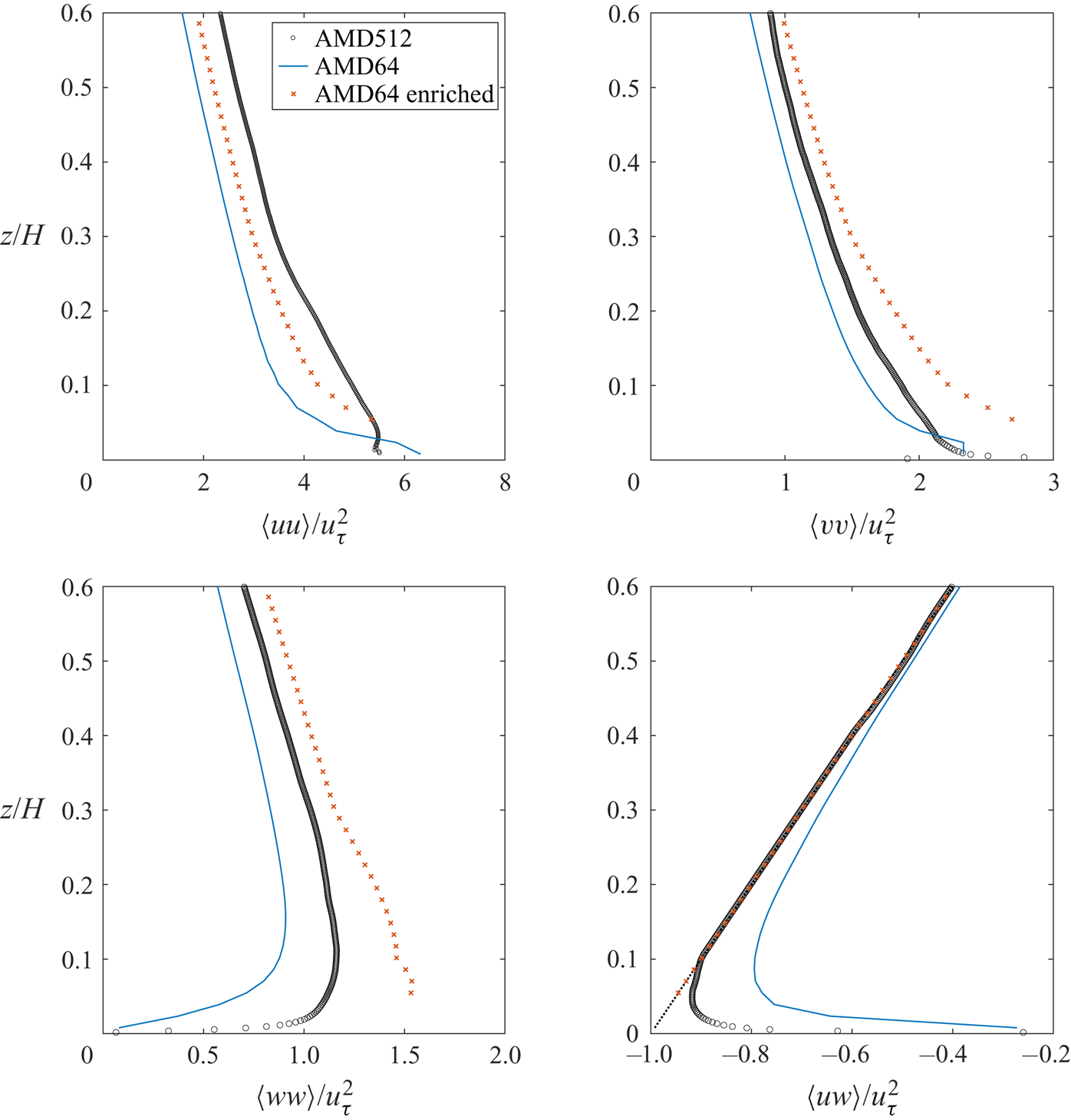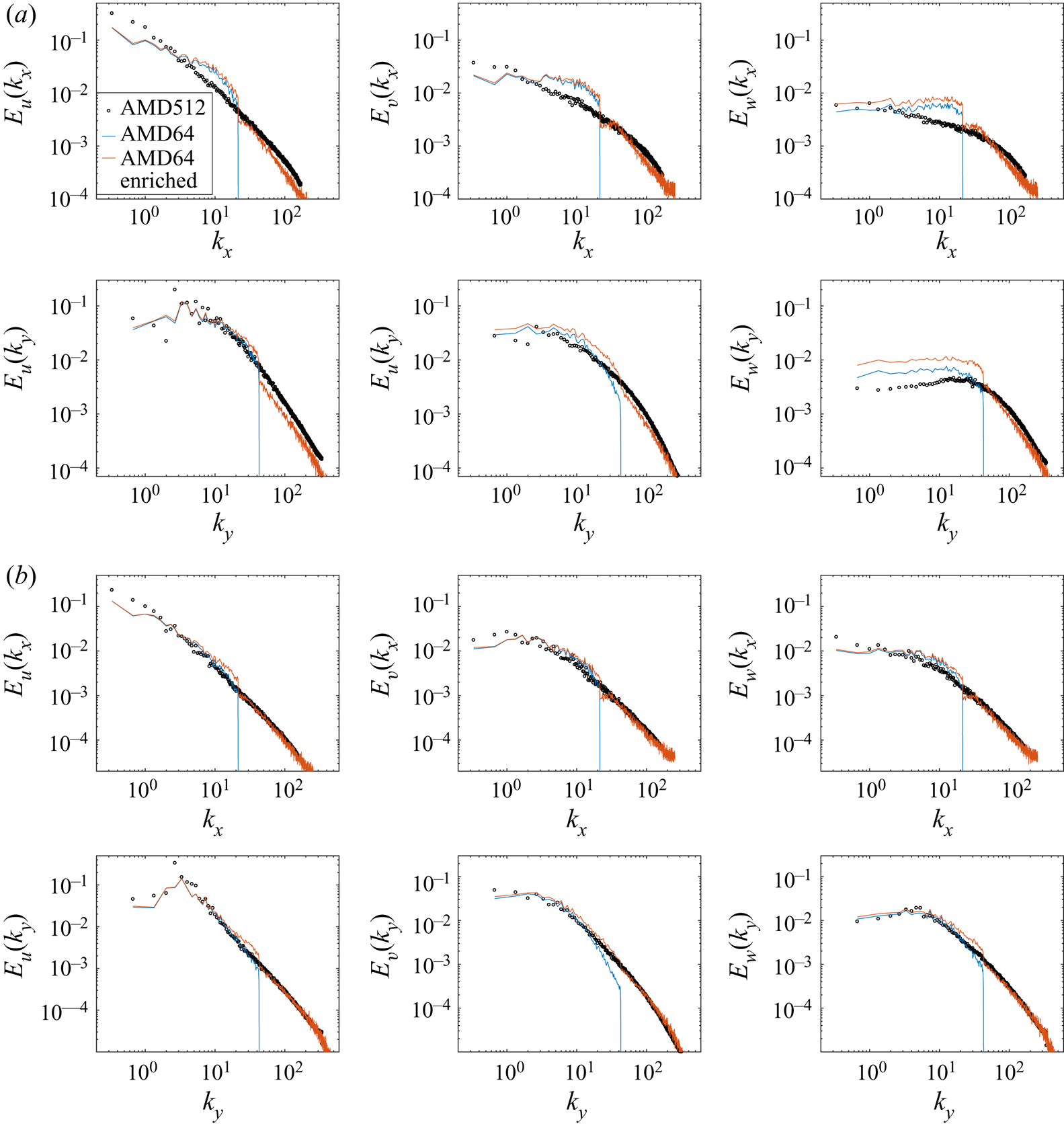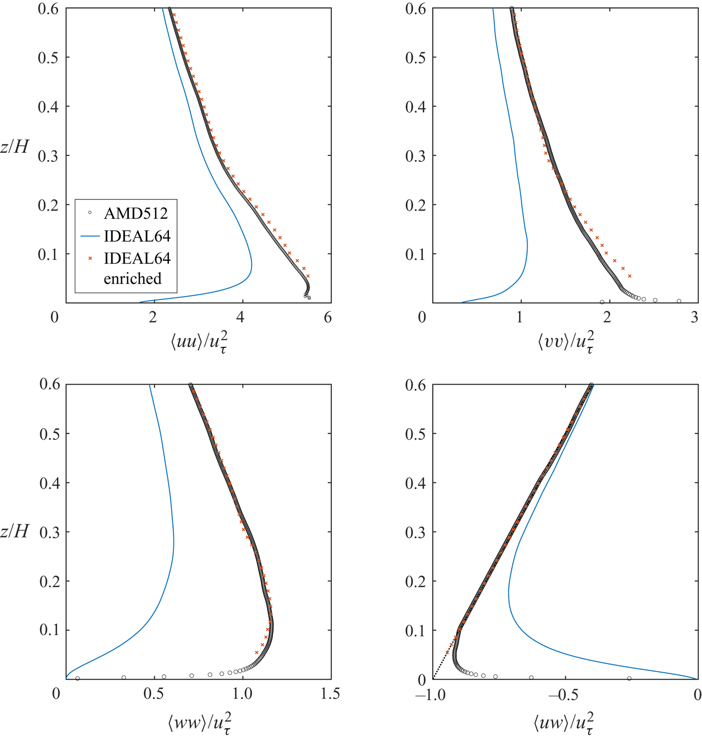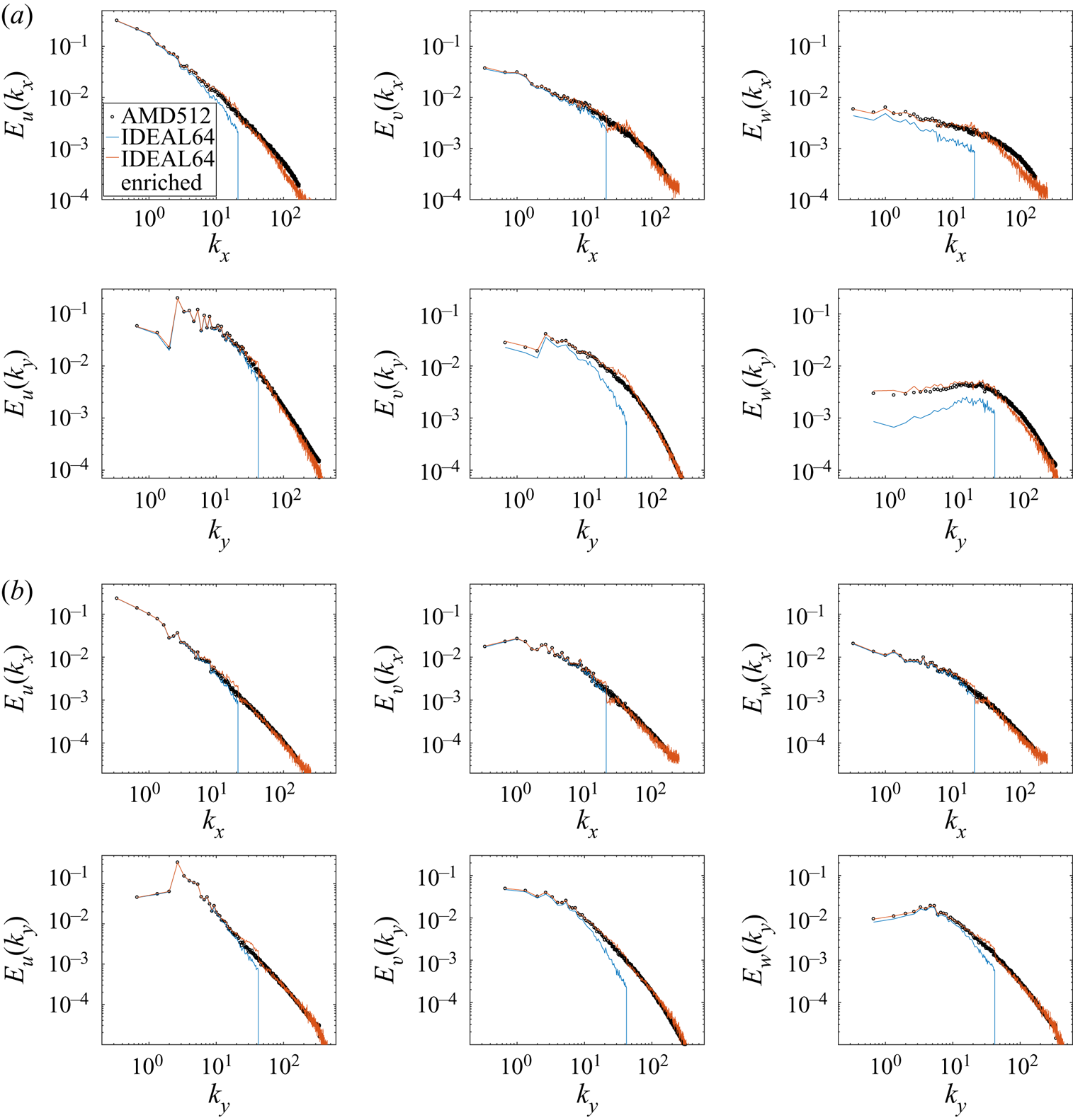

1. Introduction
It is now widely appreciated that turbulence closures based on Reynolds averaging have limited capabilities and, as noted by Spalart (Reference Spalart2015), methods that at least resolve the dynamics of the largest energy containing and geometry influenced eddies are naturally suited for a much broader range of engineering applications. Large eddy simulations (LES) employing a suitable wall-stress closure (wall-model) are among the most accurate methodologies to capture a wide range of turbulent physics including smooth body separation, unsteady wall pressure and heat-transfer effects. As detailed in recent reviews by Larsson et al. (Reference Larsson, Kawai, Bodart and Bermejo-Moreno2016) and Bose & Park (Reference Bose and Park2018), wall modelling in LES has come a long way since the first algebraic stress models developed by Deardorff (Reference Deardorff1970), Schumann (Reference Schumann1975) and subsequent inviscid rough-surface adaptation by Moeng (Reference Moeng1984) using Monin–Obukhov theory. In engineering applications wall models based on equilibrium and non-equilibrium assumptions applied to thin boundary layer equations have been deployed with reasonable success to predict skin friction and wall pressure in complex flow configurations at very high Reynolds numbers (Piomelli & Balaras Reference Piomelli and Balaras2002; Kawai & Larsson Reference Kawai and Larsson2012; Kawai & Asada Reference Kawai and Asada2013).
These recent successes of LES lead to a natural follow up question. While LES is by design meant to provide improved accuracy of moments (ensemble/statistical averages of flow variables) by explicitly resolving the geometry dependent dynamics of the largest scales of motion and modelling the effect of smaller scales, it is only capable of providing a dynamical description of turbulence with a limited spatio-temporal bandwidth. This is particularly true in canonical wall turbulence since the integral length scales vary roughly linearly with distance from the wall (Jiménez Reference Jiménez2012). In regions above the buffer layer where the effect of the viscous boundary condition is of diminishing significance, a wall-modelled large eddy simulation (WMLES) can only barely capture the integral length scale of the flow, thereby severely limiting the resolvable turbulent kinetic energy. This aspect of under resolution can easily be acknowledged by considering geophysical flows where WMLES of planetary boundary layers at  $Re_\tau \approx 10^6\text{--}10^7$ (Smits, McKeon & Marusic Reference Smits, McKeon and Marusic2011) are typically done using only
 $ {O}(10^6\text{--}10^9)$ total grid points (Brasseur & Wei Reference Brasseur and Wei2010; Jiang, Wang & Sullivan Reference Jiang, Wang and Sullivan2018) depending on the application. Turbulence enrichment, where the geometry/boundary influence large scales are solved using conventional LES and subfilter scales are synthesized, is a natural solution that can potentially enable broadband representation of turbulence at low cost in several applications including wind energy and external hydro- and aerodynamics which deal with wall pressure induced unsteady structural vibration and noise generation. Recent work in particle-laden turbulence (Mazzitelli, Toschi & Lanotte Reference Mazzitelli, Toschi and Lanotte2014; Bassenne et al. Reference Bassenne, Esmaily, Livescu, Moin and Urzay2019) also underscores the need for synthesis of scales subfilter to the LES of the carrier (fluid) phase. The enrichment model introduced in Ghate & Lele (Reference Ghate and Lele2017) tackled this aspect of LES directly via representation of small-scale turbulence using Fourier–Gabor modes together with systematic physics based modelling of the equation governing subfilter-scale flow in the context of planetary boundary layer turbulence in an a priori setting where the large scales were represented by spatial filtering of high resolution DNS or LES data. In this paper we significantly extend that approach for use in a posteriori LES.
The primary requisites of a basic turbulence enrichment are systematically introduced in § 2. In § 3 the notion of a spatially and spectrally localized Gabor mode/wavepacket is introduced and by appealing to the assumption of quasi-homogeneity of subfilter scales, we argue that these modes form an optimal numerical basis to statistically represent small-scale turbulence, and for its temporal evolution. Sections 4 and 5 comprehensively investigate the a posteriori enrichment of coarse-grid simulations of isotropic turbulence and rough-wall turbulent channel flow and identify the key strengths of the proposed model. The computational cost of the approach and salient implementation details are included in an appendix. Summarizing remarks made in § 6 are used to conclude the paper.
2. Preliminary background on turbulence enrichment
Inspired by a thought problem introduced by Wyngaard (Reference Wyngaard2010) to introduce LES, we first introduce the notion of small-scale enrichment by considering temporally stationary turbulence where resolved and subfilter are defined via a spectrally sharp filter (applied in cartesian coordinates) and denoted with superscripts  $(r)$ and
 $(s)$, respectively. Consider the incompressible, constant density Navier–Stokes equation for the total velocity field,
 $u_i$,
 \begin{equation} u_i(\boldsymbol{x},t) = u^r_i(\boldsymbol{x},t) + u^s_i(\boldsymbol{x},t), \end{equation}
where  $u^r_i$ is the spatially filtered (resolved) component of
 $u_i$:
 \begin{equation} u_i^r (\boldsymbol{x},t) = \int_{\boldsymbol{x^\prime}\in \mathcal{R}^3} u_i(\boldsymbol{x^\prime},t) G_\varDelta(\boldsymbol{x^\prime} - \boldsymbol{x})\,\textrm{d}\boldsymbol{x^\prime}. \end{equation}
Note that the filter kernel,  $G_\varDelta$, represents a filter applied at
 $\varDelta$ scale which is assumed to be spatially constant throughout this work in order to enable commutation with differentiation operators. We have
 \begin{equation} \partial_t u_i + \partial_j \left(u_i u_j \right) = -\partial_i p + \frac{1}{{Re}}\partial_{j}\partial_j u_i + \beta_i;\quad \partial_j u_j = 0, \end{equation}
where  $\partial _t$ is used to denote partial derivative in time,
 $\partial _i$ is the spatial partial derivative and
 $\beta _i$ is the additional acceleration vector needed to balance dissipation and maintain a statistically stationary state in time. We have
 \begin{gather} \partial_t u^r_i + \partial_j \left(u_i u_j \right)^r = -\partial_i p^r + \frac{1}{{Re}}\partial_{j}\partial_j u^r_i + \beta_i;\quad \partial_j u^r_j = 0, \end{gather}
 \begin{gather}\partial_t u^s_i + \partial_j \left(u_i u_j \right)^s = -\partial_i p^s + \frac{1}{{Re}}\partial_{j}\partial_j u^s_i;\quad \partial_j u^s_j = 0, \end{gather}
where we have assumed that the forcing applied is exclusively at superfilter ( $\beta = \beta ^r$) scales. Furthermore, note that the terminology
 $(u_i u_j)^r$ corresponds to the spatially filtered tensor field
 $(u_i u_j)$ and is typically expressed as
 $(u_i u_j)^r = u_i^r u_j^r + \tau _{ij}$. Here,
 $\tau _{ij} = (u_i u_j)^r - u^r_i u^r_j$ is the residual stress tensor that is the only unclosed term which is modelled in the equations governing large scales (2.4a,b). The goal of subfilter-scale enrichment as defined in this work is the generation of small scales with accurate second-order space–time correlations of the type:
 \begin{equation} c_{ij}(\boldsymbol{x},t,\boldsymbol{x^\prime}, \delta_t) = \left\langle u^s_i(\boldsymbol{x},t) u^s_j(\boldsymbol{x^\prime},t + \delta_t) \right \rangle. \end{equation}
We will separate the discussion into two parts: (a) energetics of  $u^s_i$ and (b) the temporal problem which is particularly relevant since the scale splitting and filtering procedure is explicitly defined in space and not in time (2.2).
2.1. Interscale energetics
For a spectrally sharp filter, using Parseval's theorem (which gives  $\langle u^r_i u^s_i \rangle = 0$), we see that the mean kinetic energy (KE) can be decomposed as
 \begin{equation} \left\langle u_i u_i \right\rangle = \left\langle u^r_i u^r_i \right\rangle + \left\langle u^s_i u^s_i \right\rangle. \end{equation}
Since we are interested in the dynamics of the small scales, we can further expand (2.5a,b) as
 \begin{equation} \partial_t u^s_i + u^r_j \partial_j u^s_i + u^s_j \partial_j u^r_i + u^s_j \partial_j u^s_i = -\partial_i p^s + \frac{1}{{Re}}\partial_{j}\partial_j u^s_i + \partial_j \tau_{ij};\quad \partial_j u^s_j = 0. \end{equation}
The equations that govern the kinetic energy split (2.7) for homogeneous turbulence are given as
 \begin{gather} \partial_t\left\langle \frac{u_i u_i}{2} \right \rangle = \langle \beta_i u_i \rangle - \varepsilon = \langle \beta_i u^r_i \rangle - \varepsilon, \end{gather}
 \begin{gather}\partial_t \left \langle \frac{u^r_i u^r_i}{2} \right \rangle = \langle \beta_i u^r_i \rangle + \langle \tau_{ij} \partial_j u^r_i \rangle - \varepsilon_r, \end{gather}
 \begin{gather}\partial_t \left \langle \frac{u^s_i u^s_i}{2} \right \rangle = \left[- \langle u^s_i u^s_j \partial_j u^r_i \rangle - \left( \langle \tau_{ij}\partial_j u^s_i \rangle \right) \right] - \varepsilon_s, \end{gather}
where  $\varepsilon \approx \varepsilon _s = (1/Re)(\partial _j u^s_i)( \partial _j u^s_i )$ (as
 $Re \to \infty$, fixed filter width) is the dissipation rate. The term,
 $\langle \tau _{ij} \partial _j u^r_i \rangle$ in (2.10) can be further simplified as
 \begin{align} \langle \tau_{ij} \partial_j u^r_i \rangle = - \left\langle u^r_i \partial_j \tau_{ij}\right \rangle = - \left\langle u^r_i \partial_j \left(u_i u_j \right)^r\right \rangle = - \left\langle u^r_i \partial_j \left[ \left(u_i u_j \right) - \left(u_i u_j \right)^s \right] \right \rangle = - \left\langle u^r_i \partial_j \left(u_i u_j \right)\right \rangle. \end{align}
Expanding  $(u_i u_j) = ( (u^r_i + u^s_i) ) ( (u^r_j + u^s_j) )$ in the last term and simplifying, we obtain the definition for
 $\langle \tau _{ij} \partial _j u^r_i \rangle$,
 \begin{equation} \langle \tau_{ij} \partial_j u^r_i \rangle = - \left\langle u^r_i u^r_j \partial_j u^s_i \right\rangle + \left\langle u^s_i u^s_j \partial_j u^r_i \right\rangle = \langle \tau_{ij}\partial_j u^s_i \rangle + \left\langle u^s_i u^s_j \partial_j u^r_i \right\rangle, \end{equation}
where the second equality follows by simply substituting the definition of  $\tau _{ij}$ and applying Parseval's theorem. Furthermore, note that the right-hand side term is exactly equal to the first two terms in (2.11), but with the opposite sign. Following Wyngaard (Reference Wyngaard2010), the global (reversible) interscale energy transfer for homogeneous turbulence can be defined as
 \begin{equation} \mathcal{I} = \underbrace{\left[ - \left\langle u^s_i u^s_j S^r_{ij} \right \rangle\right]}_{\mathcal{I}_1} + \underbrace{\left[- \left \langle \tau_{ij}S^s_{ij} \right \rangle \right]}_{\mathcal{I}_2 }, \end{equation}
where  $S_{ij}$ is the symmetric strain rate tensor.
We see that the interscale energy transfer between the large and small scales is due to two distinct mechanisms: (1) work done by subfilter-scale stresses against large-scale strain ( $\mathcal {I}_1$); and (2) work done by residual/subgrid stress against small-scale strain (
 $\mathcal {I}_2$). The definition above must strictly be interpreted as a global balance since it does not hold in a pointwise sense. While the second term in (2.14) can be further simplified as
 $\langle \tau _{ij}S^s_{ij} \rangle = \langle u^r_i u^r_j S^s_{ij} \rangle$ (again using Parseval's theorem), recall that the tensor
 $\tau _{ij}$ is typically modelled such that the total interscale energy transfer is statistically accurate, i.e.
 $- \langle \tau ^{mod}_{ij}S^r_{ij} \rangle = - \langle \tau _{ij}S^r_{ij} \rangle$ (Meneveau & Katz Reference Meneveau and Katz2000). For complete consistency in energetics, one might assume that an additional constraint on the enriched fields,
 $u_i^s$, is required if
 $\langle \tau _{ij}S^{s}_{ij}\rangle = \langle \tau ^{mod}_{ij}S^{s}_{ij}\rangle$. We now use Leonard's decomposition (Leonard Reference Leonard1975) to show that this is not the case. Consider
 $\mathcal {I}_2$ again,
 \begin{equation} \mathcal{I}_2 = \left\langle L_{ij} S^s_{ij} \right\rangle + \left\langle C_{ij} S^s_{ij} \right\rangle + \left\langle R_{ij} S^s_{ij} \right\rangle = \left\langle L_{ij} S^s_{ij} \right\rangle, \end{equation}
where  $L_{ij} = (u^r_i u^r_j )^r - u^r_i u^r_j$ is the Leonard stress,
 $C_{ij} = (u^r_i u^s_j + u^s_i u^r_j)^r$ is the cross-stress and
 $R_{ij} = (u^s_i u^s_j )^r$ is the resolved component of the small-scale Reynolds stress tensor. Note that the last equality in (2.15) is a consequence of Parseval's theorem. Therefore, the energy transfer due to
 $\mathcal {I}_2$ is only a function of Leonard stress which is a closed term in the LES equations (2.4a,b), and, hence, is not affected by the spatio-temporal inaccuracies associated with
 $\tau ^{mod}_{ij}$.
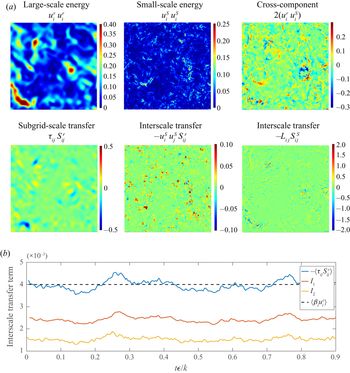
Figure 1 shows the interscale energetics for a periodic homogeneous isotropic turbulence simulation done on a  $256^3$ numerical grid at
 $Re\to \infty$ (with a subgrid-scale model). In the present discussion the role of the subgrid-scale model has been ignored since its effect is modelled as part of the nonlinear physics later. A Cartesian spectrally sharp filter is used to define large and small scales. This figure allows for the following three observations: (a) while the magnitude of the interscale transfer,
 $\mathcal {I}_1$, is substantially smaller than that of
 $\mathcal {I}_2$,
 $\mathcal {I}_1$ makes a larger contribution to the global interscale energy transfer (it is more persistently positive); (b) the small-scale kinetic energy does not appear spatially homogeneous over the entire domain but is rather well correlated with the interscale transfer that contributes to
 $\mathcal {I}_1$; and (c) the terms that contribute to
 $\mathcal {I}_2$ appear to be correlated to the cross-component of the energy,
 $u^s_i u^r_i$. While not shown here for brevity, these qualitative observations appear to be independent of the choice of the cutoff wavenumber selected in the inertial subrange.
Kinetic energy decomposition and interscale energy transfer for the homogeneous isotropic turbulence (HIT) case discussed in § 5. In subfigure (d) the red and blue regions correspond to regions where there is gain and loss in large-scale KE, respectively. In subfigures (e) and (f) the red regions depict a gain in small-scale KE whereas the blue regions indicate a loss of small-scale KE. (a) Scale decomposition for  $256^6$ forced HIT using splitting wavenumber,
 $k_{co}=16$ and (b) time history of the interscale transfer terms.

While the discussion in this section regarding interscale energy transfer has been presented from the perspective of single-point statistical measures targeted for modelling, the interested reader is referred to the substantial array of literature on interscale energetics in turbulent flows. Recent work by Doan et al. (Reference Doan, Swaminathan, Davidson and Tanahashi2018) has addressed the role of non-local vortex stretching in interscale transfer of enstrophy flux for a wide range of Reynolds numbers and Johnson (Reference Johnson2020) introduced an exact relationship between interscale energy transfer and vorticity-strain interactions. Johnson (Reference Johnson2020) shows that scale non-local vortex stretching (large-scale strain on small-scale vorticity) and strain self-amplification play a more important role in interscale transfers than scale local vortex stretching. As will be shown later in § 4, the proposed enrichment model captures the interscale tranfers via non-local vortex stretching resulting in certain vorticity alignments with large-scale strain rates that are reminiscent of the behaviour of Burgers–Townsend vortices subjected to background strain.
2.2. Temporal decorrelation of subfilter-scale turbulence
Since one of the requirements of the subfilter-scale enrichment model is accurate temporal behaviour in terms of second-order statistics, i.e.  $c_{ij}(\boldsymbol {x},t, \tau ) = \langle u_i(\boldsymbol {x},t) u_j(\boldsymbol {x},\tau ) \rangle$, it is instructive to return to (2.8a,b) and analyse its terms. However, before doing so, we will absorb the pressure nonlinearity into the other terms by using the divergence free constraint. Equation (2.8a,b) can be rewritten as
 \begin{align} \partial_t u^s_i &= - \underbrace{\left[ u^r_j \partial_j u^s_i - \left(u^r_j \partial_j u^s_i\right)^r \right]^\perp}_{{Term\ 1\ (Sweeping)}} - \underbrace{\left[u^s_j \partial_j u^r_i - \left(u^s_j \partial_j u^r_i\right)^r\right]^\perp}_{{Term\ 2\ (Straining)}} - \underbrace{\left[\partial_j \left( u^s_i u^s_j - (u^s_i u^s_j)^r \right)\right]^\perp}_{{Term\ 3\ (Nonlinear\ relaxation)}} \nonumber\\ &\quad +\underbrace{\left[\partial_j L_{ij} \right]^\perp}_{{Term\ 4\ (Leonard\ stress\ source/sink)}} + \underbrace{\frac{1}{Re} \partial_j \partial_j u^s_i}_{{Term\ 5\ (viscous\ diffusion)}}, \end{align}
where  $f_i^\perp$ is the solenoidal projection of the vector field
 $f_i$ which can be computed by solving the Poisson equation
 \begin{equation} f_i^\perp = f_i - \partial_i \phi^f;\quad \partial_j \partial_j \phi^f = \partial_i f_i. \end{equation}
It is easy to see that (2.17a,b) can be solved exactly in spectral space (homogeneity or periodicity) as  $\hat {f}_i^\perp (\boldsymbol {k}) = (\delta _{ij} - {k_i k_j}/{k_m k_m})\,\hat {f}_j(\boldsymbol {k})$ and inviscid boundary conditions can be accommodated via specifying boundary conditions on
 $\phi$.
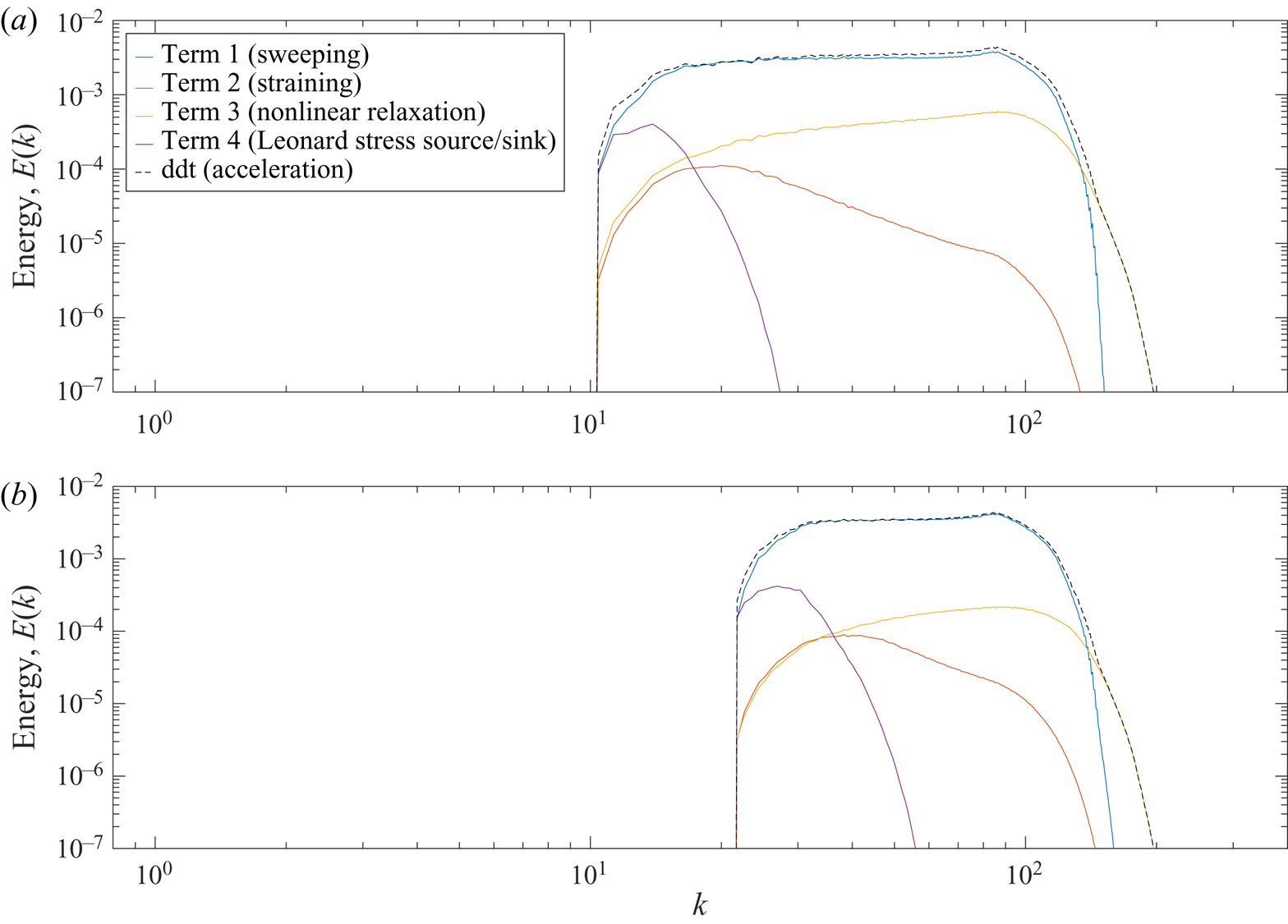
For the homogeneous isotropic turbulence (HIT) simulation shown in figure 1, we can compute the relative magnitude of each of the terms on the right-hand side of (2.16) (shown in figure 2). While this plot does not provide any information regarding the relative phase and cross-correlations among each term (sum of the mean squares of four terms does not give the energy of the total acceleration), it still suggests that the majority of the small-scale acceleration is due to the sweeping of the small scales by the large scales. The nonlinear term only becomes significant at large  $k$ and only dominates the sweeping term for
 $k>10k_{co}$, where
 $k_{co}$ is the cutoff or the scale-separation wavenumber. Note that while the energies in terms 2 and 4 are substantially smaller than the other terms, it does not necessarily mean that they do not affect temporal dynamics (in fact, as shown in the previous section, these terms cause interscale energy transfer).
Magnitude of each term on the right-hand side of (2.16) binned in spherical wavenumber bins. The magnitudes from each of the three equations are computed separately and then averaged for generating this figure. Note that the units of the  $y$-axis are non-dimensionalized using the domain length and a velocity scale determined by the energy spectrum. (a) Cutoff wavenumber,
 $k_{co} = (2/3)16$ and (b) cutoff wavenumber,
 $k_{co} = (2/3)32$.

In order to systematically study the decorrelating effect of each of the four contributors in small-scale acceleration, consider the time integral of (2.16),
 \begin{align} \int_{t}^{t+\tau} \partial_t u^s_i \,\textrm{d} t^\prime &= u^s_i(\boldsymbol{x},t + \tau) - u^s_i(\boldsymbol{x},t) = \int_t^{t+\tau} \mathcal{T}_1 \left\lbrace \boldsymbol{u}^s(\boldsymbol{x},t^\prime), \boldsymbol{u}^r(\boldsymbol{x},t^\prime) \right \rbrace \textrm{d} t^\prime \nonumber\\ &\quad + \int_t^{t+\tau} \mathcal{T}_2 \left\lbrace \boldsymbol{u}^s(\boldsymbol{x},t^\prime), \boldsymbol{u}^r(\boldsymbol{x},t^\prime) \right \rbrace \textrm{d} t^\prime + \int_t^{t+\tau} \mathcal{T}_3 \left\lbrace \boldsymbol{u}^s(\boldsymbol{x},t^\prime) \right \rbrace \textrm{d} t^\prime \nonumber\\ &\quad + \int_t^{t+\tau} \mathcal{T}_4 \left\lbrace L_{ij}(\boldsymbol{x},t^\prime ) \right\rbrace \textrm{d} t^\prime \nonumber\\ &\quad + \int_t^{t+\tau} \mathcal{T}_5 \left\lbrace Re, \boldsymbol{u}^s(\boldsymbol{x},t^\prime \right \rbrace \textrm{d} t^\prime, \end{align}
where the terms of the form  $\mathcal {T}_i$ are the five terms on the right-hand side of (2.16). Now, if we multiply both sides of the equation above by
 $u^s_i(\boldsymbol {x},t)$ and average/integrate over all
 $\boldsymbol {x}$ and
 $t$, we get (the index notation for repeated indexing is NOT applicable in this equation):
 \begin{align} c_i(\tau) &= \left\langle u^s_i(\boldsymbol{x},t) u^s_i(\boldsymbol{x},t + \tau) \right \rangle = \left\langle u^s_i(\boldsymbol{x},t) u^s_i(\boldsymbol{x},t)\right \rangle + \underbrace{\left\langle u^s_i(\boldsymbol{x},t) \int_t^{t+\tau} \mathcal{T}_1 \,\textrm{d} t^\prime \right \rangle}_{\mathcal{D}_1} \nonumber\\ &\quad + \underbrace{\left\langle u^s_i(\boldsymbol{x},t) \int_t^{t+\tau} \mathcal{T}_2 \,\textrm{d} t^\prime \right \rangle}_{\mathcal{D}_2} + \underbrace{\left\langle u^s_i(\boldsymbol{x},t) \int_t^{t+\tau} \mathcal{T}_3 \,\textrm{d} t^\prime \right \rangle}_{\mathcal{D}_3} + \underbrace{\left\langle u^s_i(\boldsymbol{x},t) \int_t^{t+\tau} \mathcal{T}_4 \,\textrm{d} t^\prime \right \rangle}_{\mathcal{D}_4} \nonumber\\ &\quad + \underbrace{\left\langle u^s_i(\boldsymbol{x},t) \int_t^{t+\tau} \mathcal{T}_5 \,\textrm{d} t^\prime \right \rangle}_{\mathcal{D}_5}. \end{align}
Note that in the high Reynolds number limit,  $Re\to \infty$, the viscous decorrelation
 $\mathcal {D}_5(\tau ) \to 0$ as long as the solution
 $u^s_i$ does not contain a finite-time singularity! The decorrelation
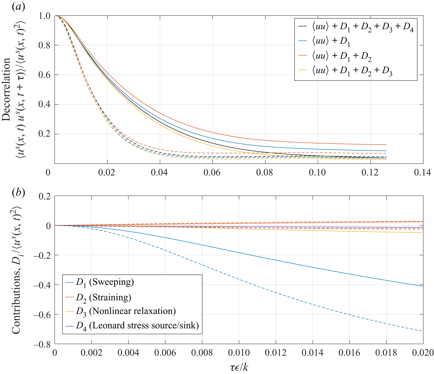
 $c_1(\tau )$ along with the four contributions from (2.19) for the HIT case are shown in figure 3. Several observations are immediately evident from these results (pertaining to the
 $k_{co} = (2/3)16$ case). The sweeping term dominates the decorrelation of small scales at early and intermediate times (
 $0.01 < \tau \varepsilon /k < 0.055$). At early times (subfigure c)
 $\tau \varepsilon /k < 0.004$, the sweeping term overpredicts the true decorrelation and the straining term corrects it by keeping the small scales correlated. This is expected since the straining term adds energy via phase alignment (rapid distortion theory (RDT)) which is consistent with the interscale energy transfer observations (see
 $\mathcal {I}_1$) made in figure 1. At late times (
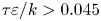 $\tau \varepsilon /k >0.045$), the nonlinear term causes non-negligible decorrelation (see subfigure a), compensating for the correlating effect of the straining term. The Leonard stress source/sink term does not appear to affect the overall statistical decorrelation of the flow field. In other words, while the term itself may be non-negligible (see figures 1 and 2), its spatial averaged counterpart does not appear to induce substantial decorrelation at time scales that are relevant to subfilter-scale motion. This is a very convenient attribute of this source term since its effect can be modelled separately using instantaneous Leonard stresses from the resolved scales. For the case with
 $k_{co} = (2/3)16$ cutoff, a large part of the overall decorrelation occurs due to the linear interactions (sweeping and straining) since the larger scales are more energetic in the
 $k_{co} = (2/3)32$ case.
Temporal decorrelation of small-scale fluctuations for the HIT case with a cutoff wavenumber. Solid lines:  $k_{co} = (2/3)16$; dashed lines:
 $k_{co} = (2/3)32$. (a) Temporal decorrelation for
 $u^s_1$ component and (b) individual contributors to decorrelation.

These observations play a key role in the development of the model for small-scale enrichment, as described in the next section.
3. Gabor mode representation
3.1. Wavelet/wavepacket representation
The Gabor modes/wavepackets employed in our formulation represent a windowed Fourier transform as will be defined later in this section. Its advantages over other types of wavelet transform are limited to the synthesis problem (as opposed to the sensing problem). In general, the use of canonical wavelets such as Daubechies (see Mallat Reference Mallat1999) family of wavelets (used in discrete wavelet transforms) provides more aggressive compression in degrees of freedom since these wavelets have physical supports that scale with wavelength, whereas Gabor wavepackets discussed here have the same fixed support for each wavelength. Due to this spatial coarsening, wavelets can provide more spatial localization than the Gabor transform/wavepacket. For a more comprehensive discussion of Gabor modes in the context of the broader class of tools that rely on wavelets (Farge & Schneider Reference Farge and Schneider2001; Goldstein & Vasilyev Reference Goldstein and Vasilyev2004), the reader is referred to Ghate (Reference Ghate2018). However, we note the following two advantages of using Gabor modes in the context of the enrichment problem.
(i) The Gabor transform is more amenable to theoretical manipulation, and ideas of Wentzel–Kramers–Brillouin (WKB) asymptotics using scale separation can easily be incorporated theoretically, which allows for easier modelling of the temporal dynamics (§ 4). In fact, substantial contributions to turbulence theory were made in the late 1990s and early 2000s using the Gabor transform (see, for example, Nazarenko, Kevlahan & Dubrulle Reference Nazarenko, Kevlahan and Dubrulle1999; Dubrulle et al. Reference Dubrulle, Laval, Nazarenko and Kevlahan2001, Reference Dubrulle, Laval, Sullivan and Werne2002; Laval, Dubrulle & Nazarenko Reference Laval, Dubrulle and Nazarenko2004).
(ii) Notion of compression in degrees of freedom does not necessarily imply reduction in computational cost. In incompressible flows the nonlinearity introduced by pressure is non-local in physical space, and can be a significant challenge in three-dimensional flows where pressure-less algorithms are not widely known. In fact, a more appropriate comparison of the wavelet-based treatment of the governing equations is that with other spectral discretizations of the full equations. Schneider & Vasilyev (Reference Schneider and Vasilyev2010) provide an excellent review of the challenges associated with wavelet discretization of incompressible Navier–Stokes equations. The notion of quasi-homogeneous (QH) regions along with some theoretical simplifications (since the oscillatory aspect is provided by Fourier basis) associated with WKB-RDT makes the treatment of this non-local nonlinearity associated with pressure, very tractable.
3.2. Quasi-homogeneity assumption
We will introduce the notion of quasi-homogeneity in the context of simulations of wall-bounded turbulence by introducing the following three length scales.
(i) The domain length scale (boundary layer height):
 $\delta$. The flow is highly inhomogeneous at this length scale due to the viscous and kinematic effects of the wall.
(ii) A coarse LES grid scale, which is also the filter width used to separate the small scales from the resolved scales:
$\varDelta$.(iii) A windowing scale
$\varDelta _w$ such that $\varDelta _w \gg \varDelta$ and $\delta \gg \varDelta _w$.


If we window the subfilter-scale (based on  $\varDelta$) field using an appropriate windowing function (here taken to be a Gaussian) of characteristic length
 $\varDelta _w$ and centred at coordinate
 $\boldsymbol {x}_0$, we obtain
 \begin{equation} \boldsymbol{u}_w(\boldsymbol{x}, \boldsymbol{x}_0, \varDelta_w) = f(\boldsymbol{x} - \boldsymbol{x}_0, \varDelta_w) \boldsymbol{u}(\boldsymbol{x}), \end{equation}
where  $\boldsymbol {u}(\boldsymbol {x})$ is an instantaneous snapshot of the velocity field. We now make the following hypothesis: for a certain choice of
 $\varDelta _w$, the vector field
 $u_w(\boldsymbol {x},\boldsymbol {x_0}, \varDelta _w)$ is locally homogeneous over length scales smaller than
 $\varDelta _w$; this will be referred to as the quasi-homogeneity assumption. If we argue that the length scale of this quasi-homogeneous region
 $(\mathcal {D}_{QH}(\boldsymbol {x}_0) \subset \mathcal {R}^3)$ is smaller than the window support, then the following deductions regarding
 $\boldsymbol {u}_w(\boldsymbol {x}, \boldsymbol {x}_0, \varDelta _w)$ immediately follow.
(i) An energy error-minimizing representation (proper orthogonal decomposition or Karhunen–Loeve expansion) of
$\boldsymbol {u}_w(\boldsymbol {x}, \boldsymbol {x}_0, \varDelta _w)$, which is also the most optimal representation (in terms of modes used), is in fact the Fourier representation (Lumley Reference Lumley1970). It is important to acknowledge that strictly speaking, this result's practical use is limited to $\boldsymbol {u}_w(\boldsymbol {x}, \boldsymbol {x}_0, \varDelta _w) \subset \mathcal {C}^2(\mathcal {D}_{QH})$ due to uniform convergence of the Fourier series.(ii) A stochastic field that is statistically equivalent (up to second order) to
$\boldsymbol {u}_w(\boldsymbol {x}, \boldsymbol {x}_0, \varDelta _w)$ for $(\boldsymbol {x} - \boldsymbol {x}_0) \in \mathcal {D}_{QH}$ can be written in terms of the stochastic Fourier–Stieltjes integral (see Batchelor Reference Batchelor1953)
(3.2)where the stochastic vector field\begin{equation} \boldsymbol{u}_s(\boldsymbol{x}) = \int_{\boldsymbol{k}\in \mathcal{R}^3} \exp ({\textrm{i}\boldsymbol{k} \boldsymbol{\cdot} \boldsymbol{x}})\,\textrm{d} \boldsymbol{Z}(\boldsymbol{k}), \end{equation}$\boldsymbol {Z}(\boldsymbol {k})$ has uncorrelated increments $\langle \textrm {d} Z_i(\boldsymbol {k}) \,\textrm {d} Z_j(\boldsymbol {k}^\prime ) \rangle = \delta (\boldsymbol {k} - \boldsymbol {k}^\prime ) \phi _{ij}(\boldsymbol {k}) \,\textrm {d}\boldsymbol {k}$, where the spectral tensor $\phi _{ij}(\boldsymbol {k})$ is the Fourier transform of the two-point Reynolds stress tensor $R_{ij}(\boldsymbol {r}) = \langle u_i(\boldsymbol {x}) u_j(\boldsymbol {x} - \boldsymbol {r}) \rangle$.(iii) Equation (3.2) can be discretized efficiently by sampling wavenumbers following the ideas of Kraichnan (Reference Kraichnan1970) and Fung et al. (Reference Fung, Hunt, Malik and Perkins1992) and as such the field
$\boldsymbol {u}_s(\boldsymbol {x})$ can be represented very efficiently in terms of $\textrm {d}\boldsymbol {Z}(\boldsymbol {k})$. However, any stochastic equivalent must also decay/attenuate to 0 for $\boldsymbol {x}$ outside of $\mathcal {D}_{QH}(\boldsymbol {x}_0)$. Thus, the random processes/modes must also carry appropriate support functions centred at $\boldsymbol {x}_0$. We will refer to these $\textrm {d}\boldsymbol {Z}(\boldsymbol {k},\boldsymbol {x}_0, \varDelta _w)$ random samplings as Gabor modes and rewrite the synthesis equation (3.2) as
(3.3)\begin{equation} \boldsymbol{u}_s(\boldsymbol{x},\boldsymbol{x}_0, \varDelta_w) = \int_{\boldsymbol{k}\in \mathcal{R}^3} \exp({\textrm{i}\boldsymbol{k} \boldsymbol{\cdot} \boldsymbol{x}}) \,\textrm{d} \boldsymbol{Z}(\boldsymbol{k},\boldsymbol{x}_0, \varDelta_w). \end{equation}


At this stage it is essential to draw the distinction between the windowed field  $\boldsymbol {u}_w(\boldsymbol {x},\boldsymbol {x}_0, \varDelta _w)$ and the synthetic field
 $\boldsymbol {u}_s(\boldsymbol {x},\boldsymbol {x}_0, \varDelta _w)$. These two fields are not the same, and the choice of
 $\textrm {d}\boldsymbol {Z}(\boldsymbol {k},\boldsymbol {x}_0, \varDelta _w)$ is not made to approximate
 $\boldsymbol {u}_w$ and as such
 $\textrm {d}\boldsymbol {Z}(\boldsymbol {k},\boldsymbol {x}_0)$ are not the proper orthogonal decomposition modes of
 $\boldsymbol {u}$. In fact, any choice of
 $\textrm {d}\boldsymbol {Z}(\boldsymbol {k},\boldsymbol {x}_0, \varDelta _w)$ that satisfies the compactness requirement for
 $\boldsymbol {u}_s(\boldsymbol {k},\boldsymbol {x}_0, \varDelta _w)$ and the requirement
 \begin{align} & \frac{\left\langle \textrm{d} Z_i(\boldsymbol{k},\boldsymbol{x}_0) \,\textrm{d} Z_j(\boldsymbol{k}^\prime, \boldsymbol{x}_0) \right \rangle}{\textrm{d}\boldsymbol{k}} = \boldsymbol{\phi}_{ij}(\boldsymbol{k}, \boldsymbol{x}_0) \nonumber\\ &\quad =\int_{\boldsymbol{r}\in\mathcal{R}^3} \left \langle u_i(\boldsymbol{x} - \boldsymbol{x}_0, \boldsymbol{x}_0) u_j(\boldsymbol{x} - \boldsymbol{x}_0 - \boldsymbol{r}, \boldsymbol{x}_0) \right \rangle \exp({-\textrm{i}\boldsymbol{k} \boldsymbol{\cdot} \boldsymbol{r}})\,\textrm{d}\boldsymbol{r} \end{align}
will result in  $\boldsymbol {u}_s(\boldsymbol {x},\boldsymbol {x}_0, \varDelta _w)$ with the same second-order spatial statistics as
 $\boldsymbol {u}_w(\boldsymbol {x},\boldsymbol {x}_0)$ as
 $\textrm {d}\boldsymbol {k} \to 0$.
3.3. Discrete Gabor modes and scale separation
We now formalize the procedure for the generation of  $\boldsymbol {u}_s$ which requires us to first identify the length scale
 $\varDelta _w$ used to window the small-scale field
 $\boldsymbol {u}$. It is obvious that for
 $\boldsymbol {u}_w(\boldsymbol {x},\boldsymbol {x}_0)$ to preserve the statistical characteristics of
 $\boldsymbol {u}(\boldsymbol {x})$ for
 $\boldsymbol {x}\in \mathcal {D}_{QH}(\boldsymbol {x}_0)$, we require
 $\varDelta _w$ to be much larger than the largest relevant scale present in
 $\boldsymbol {u}(\boldsymbol {x}),\ \boldsymbol {x} \in \mathcal {D}_{QH}(\boldsymbol {x}_0)$. This requirement is simply
 $\varepsilon = \varDelta /\varDelta _w \ll 1$ since the scale splitting filter width is
 $\varDelta$. We will refer to parameter
 $\varepsilon$ as the scale-separation parameter.
The Gabor transform of the small-scale field  $\boldsymbol {u}(\boldsymbol {x})$ is defined as:
 \begin{equation} \hat{\boldsymbol{u}}(\boldsymbol{x}_0, \boldsymbol{k}, \varepsilon) = \int_{\boldsymbol{x}\in \mathcal{R}^3} \boldsymbol{u}(\boldsymbol{x}) f\left( \varepsilon (\boldsymbol{x}_0 - \boldsymbol{x})\right) \exp ({\textrm{i} \boldsymbol{k} \boldsymbol{\cdot} (\boldsymbol{x}_0 - \boldsymbol{x})})\,\textrm{d}\boldsymbol{x}, \end{equation}
where  $f(\boldsymbol {x})$ is a smooth, compact support window function and the parameter
 $\varepsilon$ controls the window width. (This definition is slightly different from the one seen in textbooks (Debnath & Shah Reference Debnath and Shah2002) where the term
 $\exp ({\textrm {i}\boldsymbol {k} \boldsymbol{\cdot} (\boldsymbol {x} - \boldsymbol {x}_0)})$ is replaced by
 $\exp ({\textrm {i} \boldsymbol {k} \boldsymbol{\cdot} \boldsymbol {x}})$. The difference between the two is a simple modulation/phase factor
 $\exp ({-\textrm {i}\boldsymbol {k}\boldsymbol{\cdot} \boldsymbol {x}_0})$, and the definition stated here is primarily intended to make the definition consistent with (3.1) and simplify some of the properties pertaining to its differentiation.) It is easy to state the analogy between
 $\boldsymbol {\hat {u}}(\boldsymbol {k},\boldsymbol {x}_0, \varepsilon )$ and the stochastic mode,
 $\textrm {d}\boldsymbol {Z}$:
 \begin{equation} \textrm{d}\boldsymbol{Z}(\boldsymbol{x}_0, \boldsymbol{k},\varepsilon) \sim (2{\rm \pi})^3 \boldsymbol{\hat{u}}(\boldsymbol{x}_0, \boldsymbol{k},\varepsilon)\exp ({-\textrm{i}\boldsymbol{k}\boldsymbol{\cdot} \boldsymbol{x}_0}). \end{equation}
The main property that is used implicitly throughout this work is the following differentiation property:
 \begin{equation} \widehat{\frac{\partial u_i}{\partial x_j}} = \textrm{i} k_j \hat{u}_i + {O}(\varepsilon). \end{equation}
The impact of these  $ {O}(\varepsilon )$ errors on the quality of the solution is detailed in appendix A in the context of the divergence error (for two different choices of
 $\varepsilon$).
The synthesis of a small-scale field induced by the Gabor modes requires sampling of the stochastic modes  $\textrm {d}\boldsymbol {Z}(\boldsymbol {x}_0,\boldsymbol {k},\varepsilon )$. Each Gabor mode thus carries the following four variables that define it.
(i) A complex valued vector amplitude:
$\boldsymbol {a}$.(ii) A real-valued wave vector:
$\boldsymbol {k}$.(iii) A real-valued location in the physical domain:
$\boldsymbol {x}_0$.(iv) Support function
$f(\boldsymbol {x} - \boldsymbol {x}_0)$ defined in the neighbourhood of $\boldsymbol {x}_0$.


Due to the uncorrelated character of the increments/modes,  $\textrm {d}\boldsymbol {Z}$, the most appropriate choice for the support function is a trigonometric window such as a cosine window which will be used throughout this paper. This choice is largely influenced by the arguments previously made by Xiong, Nagarajan & Lele (Reference Xiong, Nagarajan and Lele2004).
In order to compute the induced velocity field at a point,  $\boldsymbol {x}$, we need to simply sum the contribution from each of the modes in the neighbourhood of
 $\boldsymbol {x}$ (its quasi-homogeneous region) where the contribution from each is simply
 $\delta \boldsymbol {u}(\boldsymbol {x}) = \boldsymbol {a}f(\boldsymbol {x} - \boldsymbol {x}_0)\exp ({\textrm {i}\boldsymbol {k} \boldsymbol{\cdot} (\boldsymbol {x} - \boldsymbol {x}_0)})$. In principle, this is a fairly expensive calculation; each quasi-homogeneous region could contain hundreds of Gabor modes, since the support function is defined by the quasi-homogeneous region it resides in, as opposed to its wavenumber. However, the calculation can be substantially accelerated by making all the modes within a quasi-homogeneous region share a single support function. As the modes travel in space, their support envelopes change depending on the quasi-homogeneous region they lie within. This assumption is consistent with the fact that quasi-homogeneous regions are defined based on flow properties, and not the Gabor modes.
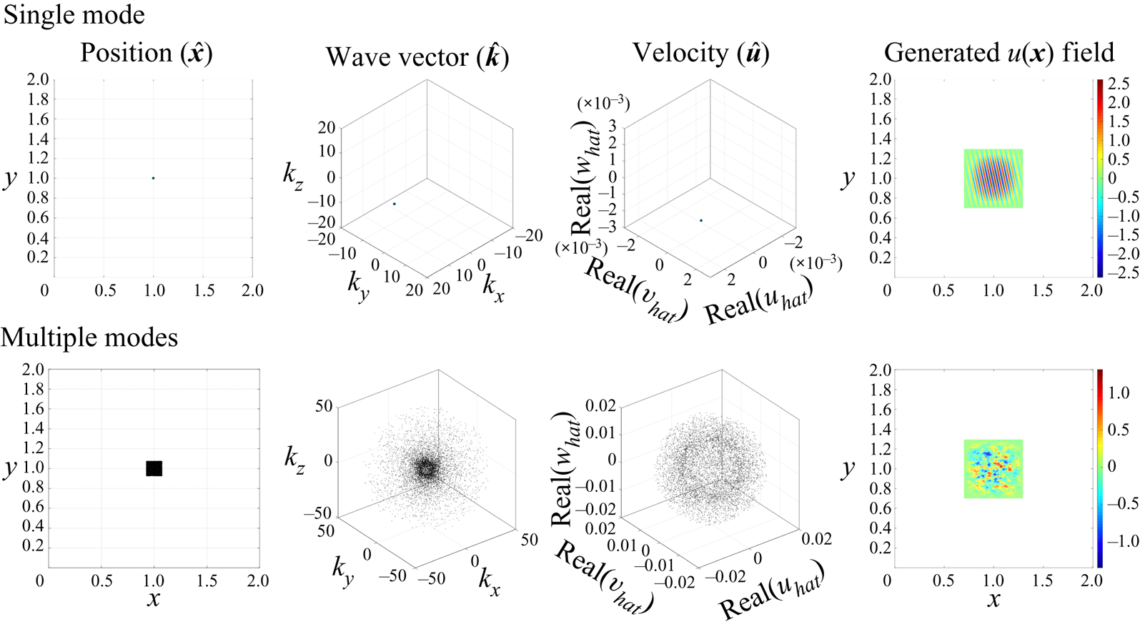
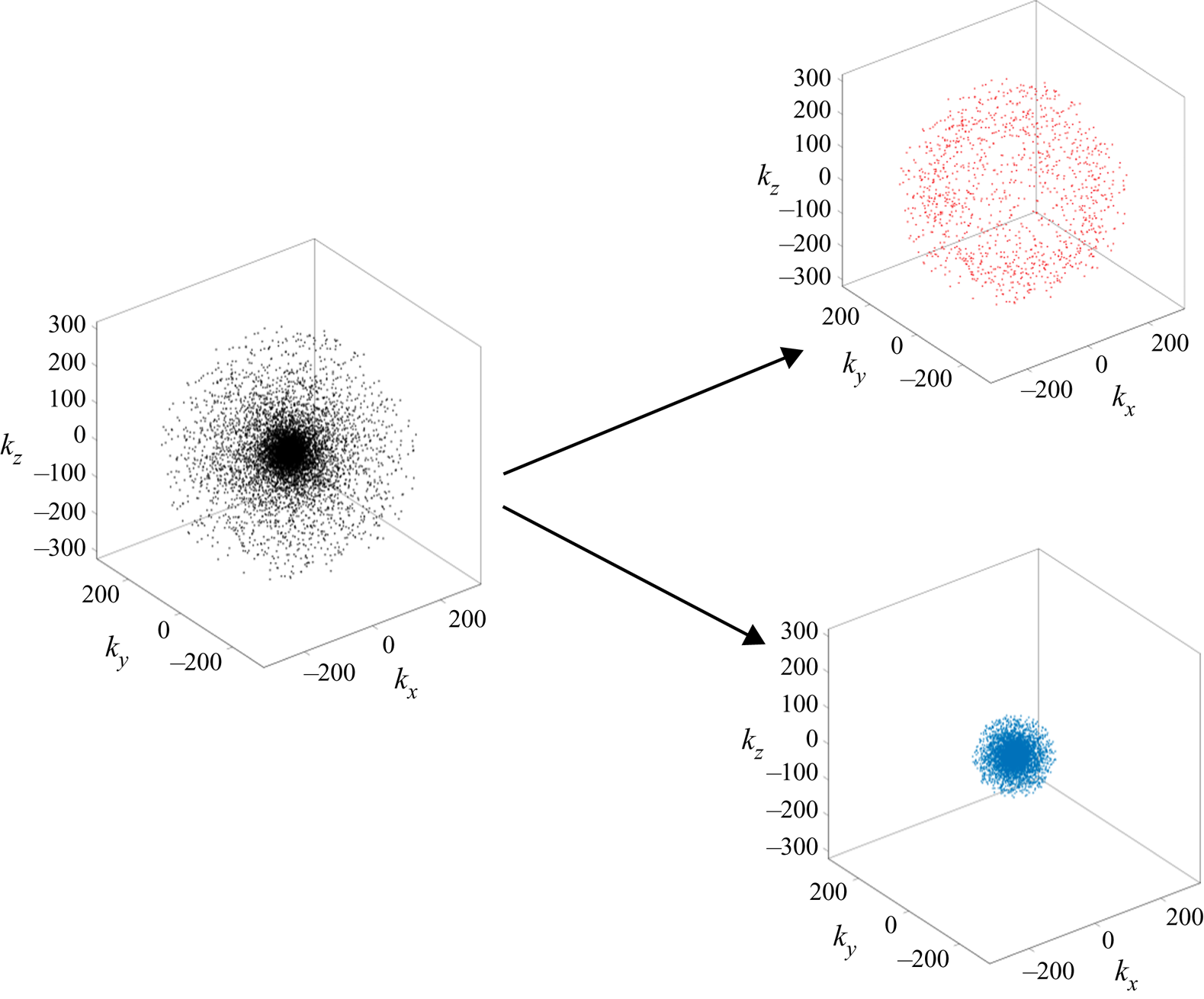
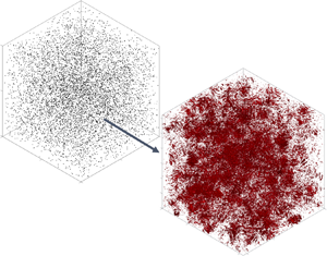
The synthesis of the velocity field for homogeneous isotropic turbulence using Gabor modes seeded in quasi-homogeneous regions is shown in figure 4. In this illustration the size of a quasi-homogeneous region is set to  $(\varDelta _{QHx},\varDelta _{QHy},\varDelta _{QHz}) = (2\varDelta _x, 2\varDelta _y, 2\varDelta _z)$, where
 $\varDelta _i$ is the coarse LES grid spacing in the
 $i$th direction. The support length is taken to be
 $(\varDelta _{wx},\varDelta _{wy},\varDelta _{wz}) = (2\varDelta _{QHx},2\varDelta _{QHy},2\varDelta _{QHz})$. This choice implies a value of
 $0.25$ for the scale-separation parameter
 $\varepsilon$ and is a theoretical upper bound for the overlapping implied by the cosine support functions. The spatial location of each mode (
 $x_j$, where
 $j$ is used to index a specific mode) within a quasi-homogeneous region is randomly sampled from a uniform distribution.
Small-scale velocity induced by Gabor modes.

The velocity induced by  $m$ total modes present within a quasi-homogeneous region centred at
 $\boldsymbol {x}_0$ at an arbitrary point
 $\boldsymbol {x}$ in the domain is given as
 \begin{align} \boldsymbol{u}_s (\boldsymbol{x},\boldsymbol{x}_0) &= \sum_{j=1}^{m} f(\boldsymbol{x} - \boldsymbol{x}_j) \boldsymbol{a}_j \exp ({\textrm{i}\boldsymbol{k}_j \boldsymbol{\cdot} (\boldsymbol{x} - \boldsymbol{x}_j)}) \approx f(\boldsymbol{x} - \boldsymbol{x}_0)\sum_{j=1}^{m}\boldsymbol{a}_j \exp({\textrm{i}\boldsymbol{k}_j\boldsymbol{\cdot} (\boldsymbol{x} - \boldsymbol{x}_j)}) \nonumber\\ &= f(\boldsymbol{x} - \boldsymbol{x}_0)\sum_{j=1}^{m} \left\lbrace\boldsymbol{a}_j \exp ({-\textrm{i}\boldsymbol{k}_j\boldsymbol{\cdot} (\boldsymbol{x}_j - \boldsymbol{x}_0)}) \right\rbrace \exp ({\textrm{i}\boldsymbol{k}_j\boldsymbol{\cdot} (\boldsymbol{x} - \boldsymbol{x}_0)}) \nonumber\\ &= f(\boldsymbol{x} - \boldsymbol{x}_0)\sum_{j=1}^{m}\boldsymbol{\tilde{a}}_j \exp ({\textrm{i}\boldsymbol{k}_j\boldsymbol{\cdot} (\boldsymbol{x} - \boldsymbol{x}_0)}). \end{align}
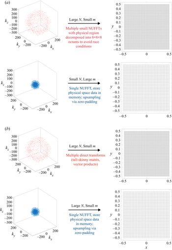
This reconstruction shows that once the modulation for each mode ( $\boldsymbol {\tilde {a}}_j = \boldsymbol {a}_j\exp (-\textrm {i}\boldsymbol {k}_j \boldsymbol{\cdot} (\boldsymbol {x}_j - \boldsymbol {x}_0))$) is calculated, calculation of the velocity field requires evaluation of the sum in the last term of (3.8). Appendix B is dedicated to developing an appropriate non-uniform fast Fourier transform (NUFFT) algorithm to calculate this sum in
 $ {O}(n\log (n))$ (
 $n$ is the number of grid points in real space), as opposed to
 $ {O}(mn)$ complexity (
 $m$ is the number of modes) implied by (3.8). (The special log-spaced structure of wavenumbers
 $\boldsymbol {k}$ can be used to substantially accelerate Greengard & Lee (Reference Greengard and Lee2004) type-I NUFFT algorithm further.) For all the problems studied in this work, the size of quasi-homogeneous regions is constant throughout the domain, including wall-bounded flows, since we assume that no grid stretching is used due to wall modelling in the coarse simulations. This assumption will also need to be revisited when Gabor modes are applied to problems with abrupt changes in direction of dominant transport (such as separated flows).
Finally, note that the initialization of the Gabor modes within quasi-homogeneous regions uses the notion of isotropically sampled modes linearly distorted by the local large-scale velocity gradient tensor (RDT) through a  $k$-dependent time scale (Mann Reference Mann1994); further details of this procedure including determination of model constants for wall-bounded flows can be found in Ghate & Lele (Reference Ghate and Lele2017).
3.4. Evolution of ordinary differential equations for Gabor modes
The equations governing temporal evolution of each Gabor mode can be obtained by considering the Gabor transform of the subfilter-scale equations (2.8a,b). However, the assumption of quasi-homogeneity requires a further decomposition of the resolved scales as
 \begin{equation} \boldsymbol{u}^{(r)}(\boldsymbol{x},t; \varDelta) = \boldsymbol{U}(\boldsymbol{x},t; \varDelta, \varDelta_{QH}) + \boldsymbol{U}^{r}(\boldsymbol{x},t; \varDelta, \varDelta_{QH}), \end{equation}
where
 \begin{equation} \boldsymbol{U}(\boldsymbol{x},t) = \int_{\boldsymbol{r}\in \mathcal{R}^3} T(\boldsymbol{r} - \boldsymbol{x}) \boldsymbol{u}^{(r)}(\boldsymbol{r},t) \,\textrm{d}\boldsymbol{r} \end{equation}
with  $T(\boldsymbol {r} - \boldsymbol {x})$ acting as the
 $\varDelta _{QH}$ scale filtering operator (equal to
 $2\varDelta$ for all the examples discussed in this paper). With this decomposition, we can derive (see appendix C) the equations that govern the evolution of each Gabor mode located within the quasi-homogeneous region
 $\mathcal {D}_{QH}(\boldsymbol {x}_0)$ over a time scale
 $t\in [0, \tau ]$ to a leading order in the scale-separation parameter,
 $\varepsilon$,
 \begin{equation} \frac{\textrm{d} a_i}{\textrm{d} t} = \left(\frac{2 k_i k_m}{k^2} - \delta_{im} \right)a_j\partial_j U_m - \nu k^2 a_i + \hat{h}_i^{\bot}, \end{equation}
where  $a_i$ is the complex valued velocity information in the Gabor mode and the eikonal equation for its wavenumber given as
 \begin{equation} \frac{\textrm{d} k_i}{\textrm{d} t} = - k_j \partial_i U_j \end{equation}
in the frame
 \begin{equation} \frac{\textrm{d} x_i }{\textrm{d} t} = U_i, \end{equation}
where  $U_i$,
 $\partial _j U_i$ is evaluated at
 $\boldsymbol {x}_0$. The term
 $\hat {h}_i^{\bot } = (\delta _{ij} - (k_i k_j)/(k_m k_m))\hat {h}_j$ comes from the nonlinear term
 $\partial _j (u_i u_j) + \partial _j (U^{r}_i u_j) + \partial _j (u_i U^{r}_j)$. The simplest model for the nonlinear term is a spectral eddy viscosity such as the one obtained using renormalization group (RNG) methods (see Canuto & Dubovikov Reference Canuto and Dubovikov1996; Laval, Dubrulle & Nazarenko Reference Laval, Dubrulle and Nazarenko2001). Under this modelling assumption, we compute
 $\hat {h}_i^{\bot }$ as
 \begin{equation} \hat{h}_i^{\bot} = - \nu_t(k) k^2 a_i, \end{equation}
where the RNG model (isotropic turbulence) for the spectral viscosity is given as
 \begin{equation} \nu_t (k) = \left(\nu^2 + 0.02\int_k^\infty q^{-2} E(q) \,\textrm{d} q \right)^{1/2} - \nu. \end{equation}
The energy spectrum  $E(k)$ in (3.15) is estimated using the Gabor modes
 $(\boldsymbol {k}, \boldsymbol {a})$. This is consistent with the assumptions and findings reported in Laval et al. (Reference Laval, Dubrulle and Nazarenko2001) where comparisons with direct numerical simulation (DNS) of three-dimensional isotropic turbulence suggest that a simple turbulent viscosity model is sufficient to obtain accurate decay rates. We further note that in the subgrid-scale (SGS) model of Dubrulle et al. (Reference Dubrulle, Laval, Sullivan and Werne2002), the authors ignore this term entirely by arguing that the subgrid-subgrid interactions are negligible. This is reasonable in their analytical model since after averaging the transport contributed by this nonlinear term is negligible. However, in our synthesis problems we have noticed that the absence of the spectral viscosity (and the implied time scale) leads to a non-physical increase in energy at high wavenumbers inconsistent with Kolmogorov inertial range (
 $-5/3$) scaling (pile-up resulting from the absence of a KE dissipation needed for finite resolution). This is consistent with the observations made by Laval et al. (Reference Laval, Dubrulle and Nazarenko2001) for isotropic turbulence, where they argue that the role of the local interactions in the nonlinear term is to weaken the intense vortices caused by the non-local interactions from the straining term. The turbulent viscosity model based on RNG is a natural choice for regularization desired in this formulation, since it gives the desired
 $k^{-4/3}$ scaling for
 $\nu _t$ as
 $k \to \infty$, and
 $k^{0}$ scaling as
 $k \to 0$. Furthermore, the implied time scale also follows the
 $k^{-2/3}$ in the inertial subrange, as is discussed further in the next subsection.
At this stage, it is important to relate the individual contributions to small-scale temporal decorrelations discussed in § 2.2 with the temporal evolution model of (3.11)–(3.13). The sweeping-effect in (2.16) is accounted for by the description of Gabor modes in a Lagrangian frame (3.13), and the straining-effect is captured by the first term on the right-hand side of (3.11) together with the eikonal equation (3.12). The nonlinear relaxation term in (2.16) is modelled using the RNG spectral viscosity closure of (3.14) and (3.15). The Leonard stress contribution which causes negligible temporal decorrelation, but results in interscale energy transfer is addressed next in § 3.5. However, it is important to emphasize at this point that these aspects of the model proposed here are helpful to justify the excellent agreement in space–time correlations of the enriched fields with reference to high resolution simulations that have previously been demonstrated for wall-bounded flows in figures 9 and 10 of Ghate & Lele (Reference Ghate and Lele2017).
3.5. Cartesian Leonard fields
The effect of the Leonard stress on the evolution of subfilter-scale fields can be accounted for by using a simple superposition argument where the full subfilter-scale flow fields are obtained as
 \begin{equation} \boldsymbol{u}^{(s)}(\boldsymbol{x},t) = \boldsymbol{u}^{Gabor}(\boldsymbol{x},t) + \boldsymbol{u}^{Leonard}(\boldsymbol{x},t), \end{equation}
and the Leonard field is simply computed as
 \begin{equation} \boldsymbol{u}^{Leonard}(\boldsymbol{x},t) = \tau_\varDelta \partial_j (L_{ij}(\boldsymbol{x},t))^\perp \end{equation}
with the Leonard stress  $L_{ij}$ introduced in (2.15). Two important observations regarding the definition (3.17) can be made.
(i) Due to the quadratic nonlinearity,
$L_{ij}$ has a Nyquist wavenumber equal to twice the Nyquist wavenumber of the large-scale fields $\boldsymbol {u}^{(r)}$. This is consistent with its contribution to the subfilter-scale acceleration shown in figure 2. More importantly, all numerical operations on $\boldsymbol {u}^{Leonard}$ (such as the projection operation implied in (3.17)) can be performed on a numerical grid that is only twice as fine as the coarse LES grid. This is in stark contrast with the numerical grid used to render the velocity fields associated with the Gabor mode contribution $\boldsymbol {u}^{Gabor}$ which requires a numerical mesh that is at least a factor of 8 finer than the coarse LES mesh.(ii) The time scale
$\tau _\varDelta$ is exclusively a function of the filter length associated with the coarse LES fields $\boldsymbol {u}^{(r)}$. It can be modelled as
(3.18)where\begin{equation} \tau_\varDelta = \frac{c_{LEO}}{k_\varDelta \sqrt{\int_{k_\varDelta}^{\infty} E(k)\,\textrm{d} k}}, \end{equation}$k_\varDelta$ is the Nyquist wavenumber of the large scales $\boldsymbol {u}^{(r)}$ and $c_{LEO}=1.2$ is a model constant, and the spectrum $E(k)$ can be approximated using the Gabor modes. The reader is referred to recent work by Kelly (Reference Kelly2018) who reviews the different time scales used in the literature, and the choice in (3.18) corresponds to $p=0$ in generic form given in Kelly (Reference Kelly2018). Note that the constant $c_{LEO}$ is a calibrated (using isotropic turbulence) model constant and does not depend on the wavenumber as long as the scale separation is performed in the inertial subrange.


4. Homogeneous isotropic turbulence
4.1. Description of baseline simulations
Consider a forced HIT LES at  $Re\rightarrow \infty$, performed on a sequence of numerical grids starting from
 $32^3$ through
 $512^3$. The absence of molecular viscosity necessitates the use of a robust subgrid-scale model to balance the production of turbulent kinetic energy without causing aliasing of resolvable fields. All simulations reported in this section were performed using Fourier-collocation with
 $2/3$rd dealiasing (explicit filtering), and used the Sigma (Nicoud et al. Reference Nicoud, Toda, Cabrit, Bose and Lee2011) SGS closure with a grid independent model constant of
 $1.3$. The flow is forced in Fourier space by choosing random modes at each time step within
 $k=1$ and
 $k=2$ spherical shells, thereby prescribing the overall turbulent dissipation rate for the simulation (see Carati, Ghosal & Moin (Reference Carati, Ghosal and Moin1995) for details). The parameters that characterize the isotropic turbulence studied in this section are provided in table 1. The domain size is the conventional
 $2{\rm \pi} \times 2{\rm \pi} \times 2{\rm \pi}$, and the simulation is allowed to reach an equilibrium state by an initial spin up time of approximately
 $10 q/\varepsilon$ (
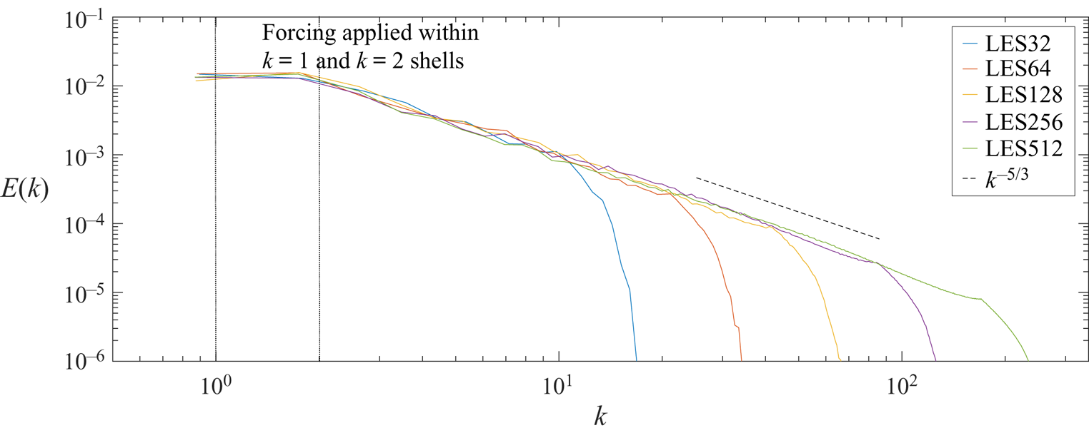
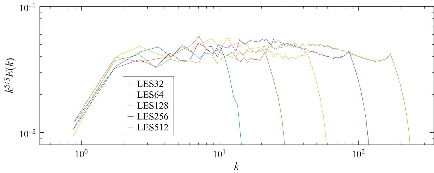
 $q$ is the turbulent kinetic energy) prior to performing any analysis. Figure 5 shows that all simulations exhibit reasonable scale invariance in terms of spatial distribution of kinetic energy (since production is completely resolved for all cases), with some departure from the
 $-5/3$ slope occurring beyond a wavenumber that corresponds to approximately half of the Nyquist wavenumber (figure 6).
Kinetic energy spectrum for LES grids from  $32^3$ to
 $512^3$.

Compensated kinetic energy spectrum for LES grids from  $32^3$ to
 $512^3$.

Characteristic parameters for the forced HIT simulations.

Gabor modes are seeded within  $32^3$ simulation and the effective full velocity fields are visualized on a
 $256^3$ numerical grid, which implies a factor of
 $8$ enrichment (in each spatial dimension), and the independent LES simulation performed on a
 $256^3$ numerical grid will serve as the benchmark for comparisons. A total of
 $512$ Gabor modes are used in each quasi-homogeneous region (
 $2\times 2\times 2$ LES cells) implying a use of
 $88\,\%$ fewer spatial degrees of freedom than in the
 $256^3$ case. Such a comparison requires the ability to interpolate the
 $32^3$ LES fields on to the
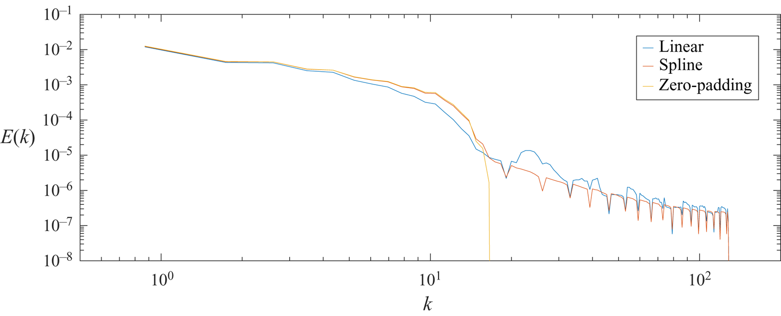
 $256^3$ grid and figure 7 shows that while linear interpolation is overly dissipative, using cubic splines essentially eliminates this artificial energy loss. The applications discussed in this work use zero-padding in Fourier space for upsampling in periodic directions (sinc-interpolation), and cubic spline interpolation for non-periodic directions.
Filtering effect of interpolation of  $32^3$ field to the
 $256^3$ grid. Energy losses are approximately
 $14\,\%$ (linear),
 $2.5\,\%$ (spline) and
 $0\,\%$ for zero-padding.

4.2. Gabor mode enriched solutions
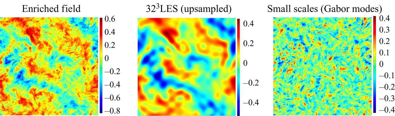
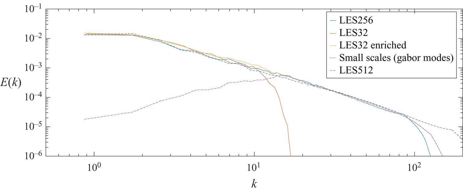
Figure 8 shows an instantaneous snapshot of the flow fields generated via Gabor mode enrichment of the  $32^3$ LES. The resulting kinetic energy spectrum (figure 9) shows the spectral extrapolation provided by the small scales induced by Gabor modes. The
 $512^3$ LES results are also included for reference to explain that the slight overprediction of KE in the enriched fields at high wavenumbers is not unphysical; the
 $256^3$ LES suffers from some artificial decay in energy at very high wavenumbers due to inaccuracies in SGS modelling. The remaining observations can be summarized as follows.
Instantaneous snapshot of  $v$ velocity field on an arbitrary
 $x$–
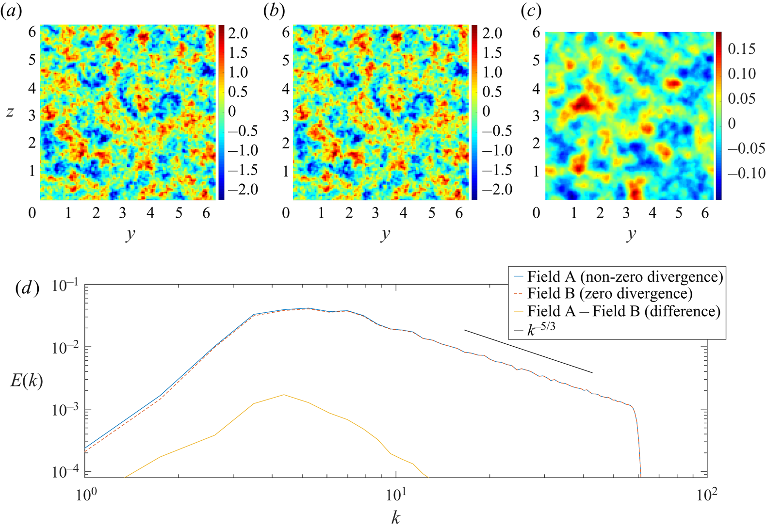
 $y$ plane. Results can be compared with figure 13(a–c).

Kinetic energy spectrum for the forced HIT simulations with Gabor mode enrichment. Results can be compared with figure 13(d).

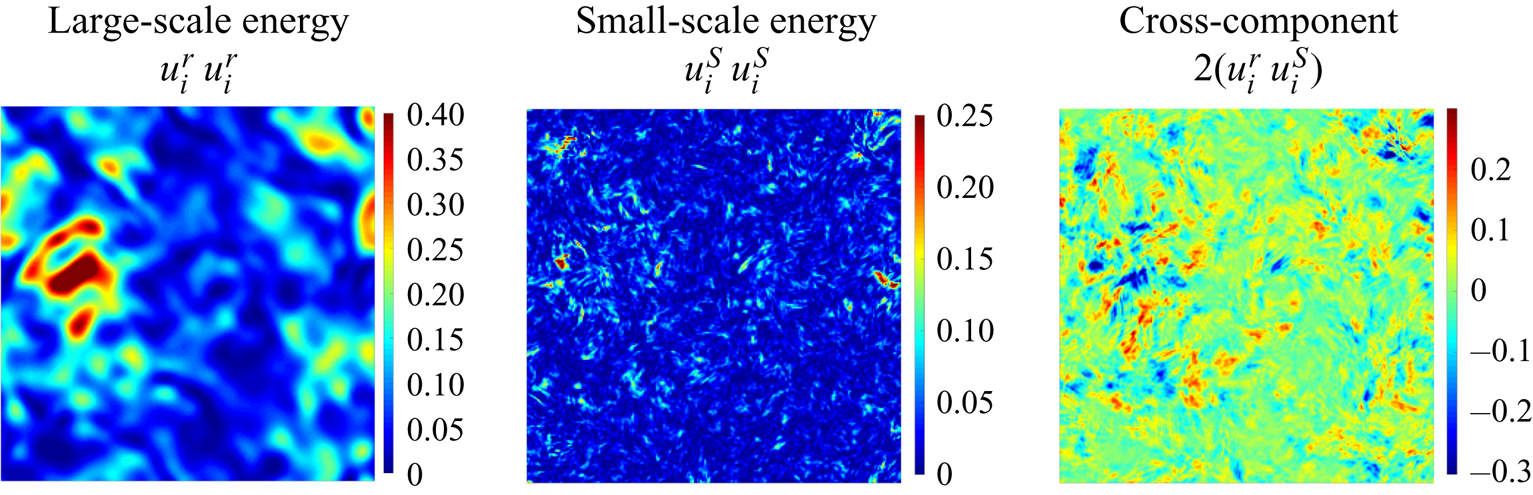
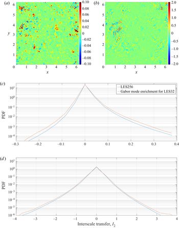
Figure 10 shows that small-scale kinetic energy induced by Gabor modes has localized peaks that occur due to intense straining by the large scales. This is consistent with the observations made in § 1. The instantaneous interscale energy transfers,  $\mathcal {I}_1$ and
 $\mathcal {I}_2$ (2.14), are shown in figure 11 to demonstrate the tight coupling observed between the
 $32^3$ LES and the enriched Gabor modes. The mean values for
 $\mathcal {I}_1$ and
 $\mathcal {I}_2$ are
 $0.0025$ and
 $0.0018$, respectively, in excellent agreement with the expected true values. Again, it is interesting to observe the strong correlation seen between small-scale kinetic energy and
 $\mathcal {I}_1$, and cross-component of the energy and
 $\mathcal {I}_2$. The interscale energy transfer
 $\mathcal {I}_2$ is primarily a consequence of the Gabor modes generated by the Leonard stress term in their evolution equations. The effect of these modes is localized near the filter wavenumber (
 $k_{co}=(2/3)16$). Spectral enrichment methods such as kinematic simulations of Flohr & Vassilicos (Reference Flohr and Vassilicos2000) create excellent spectral extrapolations (similar to present results), but do not capture any interscale energy transfers since Fourier modes lack spatial localization seen in Gabor modes. Figures 11(c) and 11(d) compare the two interscale transfer rates with the true results based on filtering of the
 $256^3$ reference LES. The results show very promising agreement, with any quantitative differences limited to a slight overprediction of intermittency (kurtosis) in the Gabor mode enriched case. Note that such quantitative differences in higher-order statistics are not unexpected since the reference case is not grid converged (and is not a DNS), and the SGS model does contaminate the smallest scales resolved in the
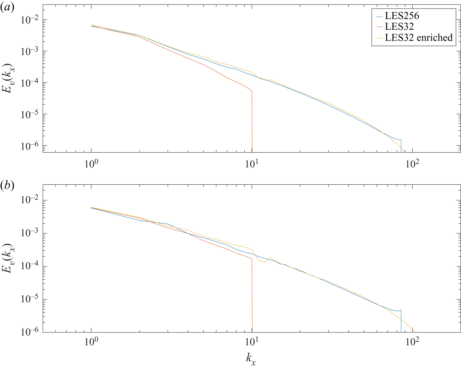
 $256^3$ LES. One-dimensional spectra for
 $u$ and
 $v$ components are shown in figure 12. The overall agreement with the
 $256^3$ LES is reasonable. The discrepancies seen near
 $k_{co} \approx (2/3)16$ can be attributed to the cartesian (tensor product) nature of the
 $32^3$ LES and the spherical nature of
 $\boldsymbol {k}$-vectors in the enriching Gabor modes. Figure 13 shows two-dimensional spectra for
 $u$ and
 $w$ components. The box drawn using red dashes is the spectral reach of the
 $32^3$ LES (corresponding to
 $k_{co} =(2/3)16$). The black contour levels are made using
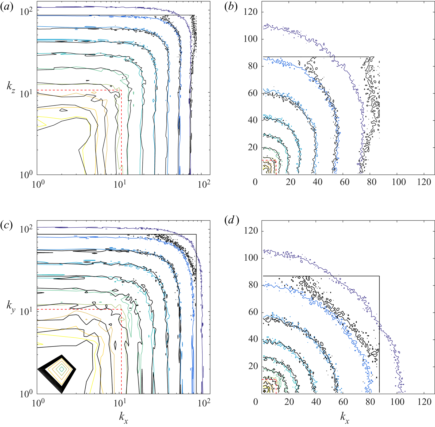
 $256^3$ LES data and the coloured levels are generated using enriched LES data. Figures 13(c) and 13(d) exhibit a
 $90^{\circ}$ rotational invariance, whereas figures 13(a) and 13(b) notably lack this invariance, consistent with the symmetries expected in isotropic turbulence (
 $u$ component has a larger integral length scale in the
 $x$ direction compared to the
 $y$ and
 $z$ directions); small scales induced by Gabor modes preserve these global symmetries. Note that the
 $256^3$ LES uses
 $2/3$rd dealiasing, which is not needed in the enriched LES. These results reinforce the excellent comparison seen in the energy spectrum. The ability of the
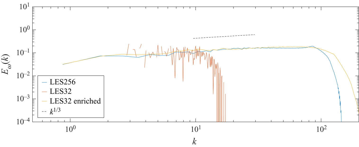
 $32^3$ LES in predicting accurate two-point correlations at large scales is noted. The enstrophy spectrum is compared in figure 14. The large noise level in
 $32^3$ LES is a consequence of reduced sampling size, but the effective enstrophy of the enriched LES compares quite well with the enstrophy resolved by the
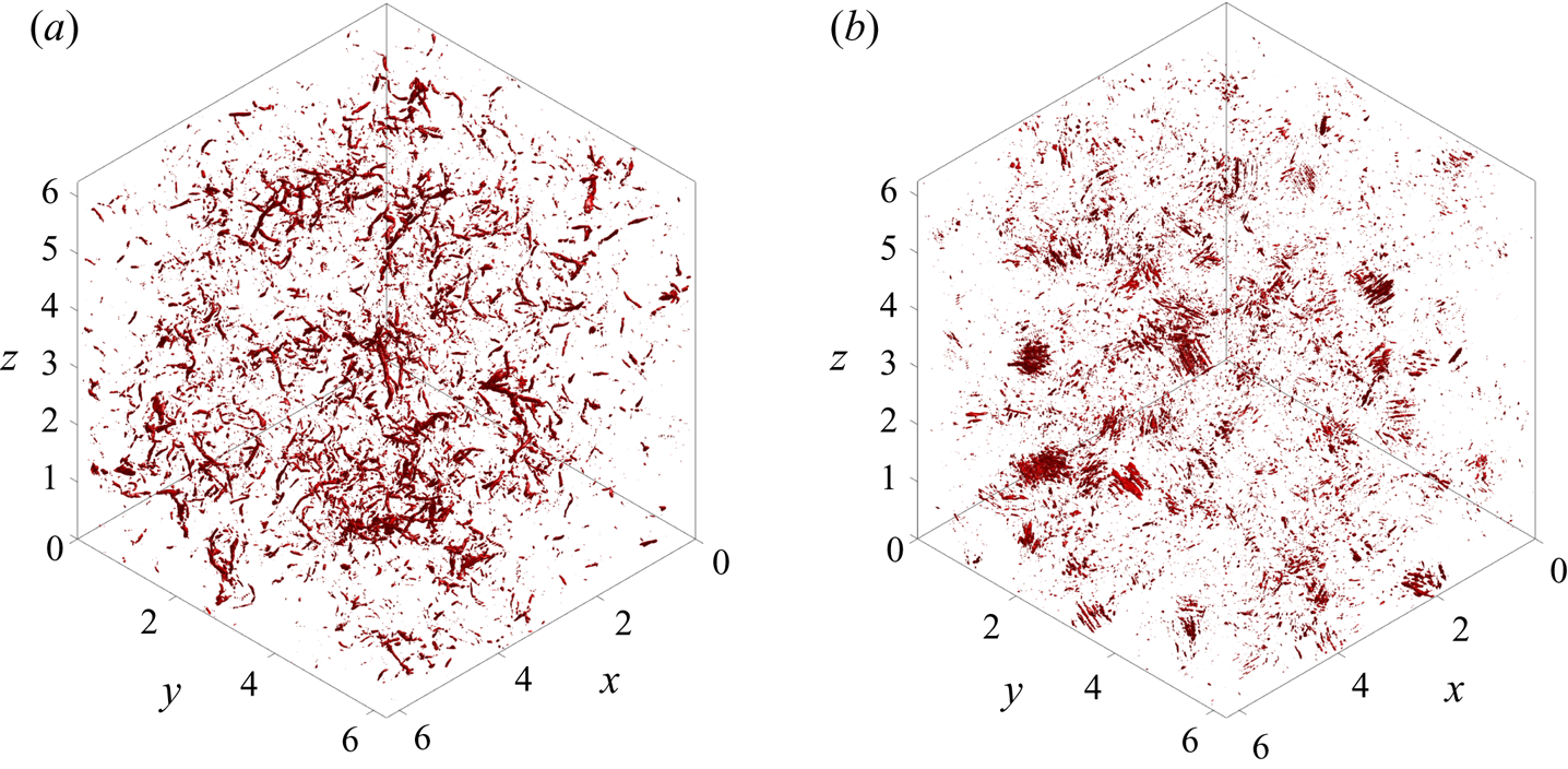
 $256^3$ LES. However, this global picture of vorticity can be quite misleading since it does not provide any insight regarding spatial coherence of the vorticity field. Figures 15 and 16 show the isocontours of vorticity magnitude in the simulated domain at contour levels of
 $150\varepsilon /q$ and
 $210\varepsilon /q$, respectively. These values are approximately
 $2.1$ and
 $3$ times the root mean square vorticity magnitude for the
 $256^3$ LES. It is clear that a simulation at
 $32^3$ size does not resolve any strong vorticity of this magnitude. However, these vorticity isosurfaces help identify two notable deficiencies in the Gabor mode induced velocity fields.
(i) The RDT-linearization in Gabor mode evolution equations leads to numerous thin vortex filaments; however, the effect of nonlinear terms which cause mutual distortion and entanglement (She, Jackson & Orszag Reference She, Jackson and Orszag1990) is noticeably absent. Laval et al. (Reference Laval, Dubrulle and Nazarenko2001) claim that vortex reconnection is essentially a nonlinear process in which local (in scale space) interactions play an important role. Instead, the spectral viscosity used here simply prevents uninhibited stretching implied by the RDT-like terms.
(ii) The effect of quasi-homogeneous regions is very evident in the Gabor mode induced vorticity. While the thin filaments in the LES have a radii of the order of grid resolution (Kolmogorov scale in DNS), their long lengths imply a large spatial coherence. We consider the preferential orientation of the subfilter-scale vorticity
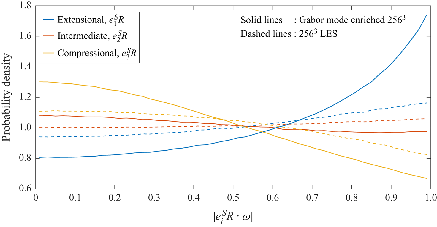
$\boldsymbol {\omega }_S$ with the largest eigenvalue of the large-scale ($32^3$ LES) strain rate tensor $\boldsymbol {S}_{R}$ as shown in figure 17. It is clear that the fine-scale vorticity in the enriched case lacks some of the true physics which appears to be more nuanced and complex (see figure 16a). The enriched vorticity appears to primarily consist of elongated cylindrical structures, reminiscent of Burgers–Townsend vortices (Townsend Reference Townsend1951). We observe that this subfilter-scale vorticity contained in Gabor modes is consistent with the RDT-type arguments made in vortex-based closures (Pullin & Saffman Reference Pullin and Saffman1994; Kosović Reference Kosović1997; Misra & Pullin Reference Misra and Pullin1997) for the full subgrid-scale stress tensor. Such closure models attempt to model the probability density of the subfilter vortex orientation; this statistical information is naturally present in Gabor modes due to the statistical equivalence requirement given in (3.4).


Instantaneous kinetic energy resolved by the  $32^3$ LES and the small-scale energy induced by Gabor modes.

Instantaneous energy injected into the small scales induced by Gabor modes. (a) Instantaneous transfer ( $\mathcal {I}_1$),
 $- u^s_i u^s_j S^r_{ij}$; (b) instantaneous transfer (
 $\mathcal {I}_2$),
 $-L_{ij}S^s_{ij}$; (c) probability density function (PDF) of
 $\mathcal {I}_1 = -u^s_i u^s_j S^r_{ij}$ and (d) PDF of
 $\mathcal {I}_2 =-L_{ij}S^s_{ij}$.

One-dimensional  $k_x$ spectra. For (a)
 $u$ component and (b)
 $v$ component.

Two-dimensional spectra for  $u$ and
 $w$ components. The contour levels are logarithmically equispaced between
 $10^{-8}$ and
 $10^{-3.5}$. Black lines:
 $256^3$ LES; coloured lines:
 $32^3$ LES enriched with Gabor modes. (a)
 $k_x - k_y$ spectrum for
 $u$ (log spacing); (b)
 $k_x - k_y$ spectrum for
 $u$ (linear spacing); (c)
 $k_x - k_y$ spectrum for
 $w$ (log spacing) and (d)
 $k_x - k_y$ spectrum for
 $w$ (linear spacing).

Enstrophy spectrum for the forced HIT simulations.

Isocontours of instantaneous absolute vorticity. Contour level is  $150\varepsilon /q$. The
 $32^3$ LES does not capture any features at this vorticity level. (a)
 $256^3$ LES and (b)
 $32^3$ LES enriched with Gabor modes.

Isocontours of instantaneous absolute vorticity. Contour level is  $210\varepsilon /q$. The
 $32^3$ LES does not capture any features at this vorticity level. (a)
 $256^3$ LES and (b)
 $32^3$ LES enriched with Gabor modes.

Preferential alignment of the small-scale vorticity with the largest eigenvalue of the large-scale strain rate tensor.

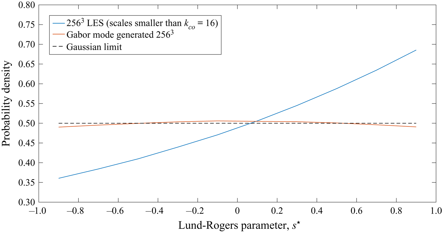
Finally, it is interesting to observe that the small-scale strain rate as measured in terms of the Lund–Rogers parameter (Lund & Rogers Reference Lund and Rogers1994) shown in figure 18 suggests that the field has Gaussian statistics. This appears to be consistent with the observation by Pullin & Saffman (Reference Pullin and Saffman1998) who note that volume-filling ensembles of Townsend–Burgers’ vortices give poor results for the higher-order moments of the longitudinal velocity derivatives for isotropic turbulence. In regards to the LES results shown in figure 17, note that while the  $256^3$ LES which captures the entire nonlinearity at small scales also shows some preferential alignment, its probability density function does not present a strong peak at the perfectly aligned state as would be expected from a highly resolved direct numerical simulation for a finite Reynolds number case. We note that the widely accepted result regarding the alignment of vorticity with the eigenvector of strain rate with the second largest eigenvalue (Ashurst et al. Reference Ashurst, Kerstein, Kerr and Gibson1987; Cantwell Reference Cantwell1992) should not be confused with the observation reported in figure 17 which only considers the non-local (large-scale) straining of vorticity (Hamlington, Schumacher & Dahm Reference Hamlington, Schumacher and Dahm2008). Other spectral enrichment methods relying on global Fourier modes (Flohr & Vassilicos Reference Flohr and Vassilicos2000) fail to capture any of these interactions and the small scales are generated due to an entirely incoherent vorticity distribution.
Probability distribution of small-scale strain state as measured according to the parameter  $s^\star = {-3\sqrt {6} \alpha \beta \gamma }/{(\alpha ^2 + \beta ^2 + \gamma ^2 )^{3/2}}$ (Lund & Rogers Reference Lund and Rogers1994), where
 $\alpha$,
 $\beta$ and
 $\gamma$ are the eigenvalues of the strain rate tensor (small scale). While the LES solution shows preference towards the axisymmetric extension, the Gabor mode induced small-scale strain rate is largely Gaussian.

5. Half-channel at $Re \rightarrow \infty$

5.1. Problem description and quality of coarse-grid LES
The second problem studied is a canonical wall-bounded flow simulated as a rough-wall turbulent half-channel (of height  $H$), with slip boundary conditions at the top (
 $z=H$) and implied no-slip (stress condition for WMLES) boundary conditions at the bottom (
 $z=0$). Roughness length scale
 $z_0$ is taken to be
 $10^{-4}H$. The domain size simulated for all cases is
 $(6{\rm \pi} \times 3{\rm \pi} \times 1)H$; such a large horizontal domain is needed due to the presence of very large streamwise-elongated coherent structures (also referred to as very large-scale motions or VLSMs) of size
 $ {O}(10)$ boundary layer thickness that occur at high Reynolds numbers (del Álamo & Jiménez Reference del Álamo and Jiménez2003; Tomkins & Adrian Reference Tomkins and Adrian2003; Balakumar & Adrian Reference Balakumar and Adrian2007; Hutchins & Marusic Reference Hutchins and Marusic2007). Furthermore, regardless of the total number of grid points used, the cell aspect ratios for all the reported WMLES is fixed at
 $2{\rm \pi} \times {\rm \pi} \times 1$, implying a smaller grid spacing in the spanwise direction (
 $y$) than the streamwise direction (
 $x$). Note that these choices of domain length and cell aspect ratio are consistent with the findings of Lozano-Durán & Jiménez (Reference Lozano-Durán and Jiménez2014) and Stevens, Wilczek & Meneveau (Reference Stevens, Wilczek and Meneveau2014). The simulations compared in this section correspond to the following cases.
(i) Coarse scale (low resolution) LES: computed using
$192 \times 192 \times 64$ grid points and three SGS models. Anisotropic minimum dissipation (AMD) model of Rozema et al. (Reference Rozema, Bae, Moin and Verstappen2015) using a model constant of $1/{\rm \pi} ^2$ in the $x$ and $y$ directions (note that due to $2/3$rd dealising, the filter width is taken as $\varDelta _{filt} = (3/2)\varDelta _{grid}$) and $\sqrt {0.30}$ for the $z$ direction. These choices for the constants are consistent with those reported in Rozema et al. (Reference Rozema, Bae, Moin and Verstappen2015) and Bae (Reference Bae2018); while we use a sixth-order compact finite difference scheme in $z$, the formal order of accuracy is still second order in wall-bounded flows due to the cosine-transform based Poisson solver. Although this region of second-order accuracy is highly localized within the first few near-wall cells, the use of Poincare constant corresponding to second-order numerical accuracy is a conservative choice. Our numerical experiments suggest very low sensitivity to this choice of the constant in the $z$ direction. The results obtained for this simulation case are labelled as AMD64.(ii) Coarse scale (low resolution) LES computed using a
$384 \times 384 \times 128$ grid and the AMD subgrid-scale model. This second low resolution simulation is used to address some of the deficiencies seen in Gabor mode enrichment of the $192 \times 192 \times 64$ simulations. The results obtained for this simulation case are labelled as AMD128.(iii) Fine-scale (high resolution) LES: computed using
$1536 \times 1536 \times 512$ grid points with the anisotropic minimum dissipation SGS model. This case will serve as a benchmark for comparison with Gabor mode enriched LES and will be denoted as AMD512.(iv) Enriched LES: each quasi-homogenenous region (
$2\times 2\times 2$ grid cells) of the coarse LES is enriched with $512$ Gabor modes. Induced flow fields are evaluated on a $1536 \times 1536 \times 512$ grid.





In addition to the simulations listed above we further include results obtained by enriching the filtered AMD512 fields; this case will be labelled as IDEAL64. These fields are obtained by explicitly filtering the high resolution LES data to the coarse resolution LES grids using sharp spectral filters in  $x$ and
 $y$, and the Pade least squares filter (Spyropoulos & Blaisdell Reference Spyropoulos and Blaisdell1996) in the wall-normal,
 $z$ direction.
Since we are considering the infinite Reynolds number limit, the large eddy simulations discussed here replace the no-slip boundary condition at  $z=0$ by a shear stress boundary condition where the shear stress is computed using a simple equilibrium wall model of the form (Yang, Park & Moin Reference Yang, Park and Moin2017)
 \begin{equation} \tau_{xz} = \left[\frac{\kappa u_{\parallel}}{\ln (z_{match}/z_0) }\right]^2\frac{u_{match}}{u_\parallel};\quad \tau_{yz} = \left[\frac{\kappa u_{\parallel}}{\ln (z_{match}/z_0) }\right]^2\frac{v_{match}}{u_\parallel}, \end{equation}
where  $\kappa$ is the von Karman constant,
 $u_{match}$ and
 $v_{match}$ are the instantaneous
 $x$ and
 $y$ velocity components at a fixed wall-normal location
 $z_{match}$ and
 $u_\parallel = \langle \sqrt {u_{match}^2 + v_{match}^2} \rangle$. As highlighted by Kawai & Larsson (Reference Kawai and Larsson2012), the choice of
 $z_{match}$ largely influences the so-called log-layer mismatch (LLM). While certain adjustments in the near-wall region are commonly used by the atmospheric science community for Ekman layers (Brasseur & Wei Reference Brasseur and Wei2010; Sullivan & Patton Reference Sullivan and Patton2011), Bou-Zeid, Meneveau & Parlange (Reference Bou-Zeid, Meneveau and Parlange2005) and Yang et al. (Reference Yang, Park and Moin2017) have proposed to use either spatial or temporal filtering of velocity fields (
 $u_{match}$ and
 $v_{match}$), and shown that when
 $z_{match} = \varDelta _z/2$ (first off the wall grid point), the filtering operation largely eliminated the log-layer mismatch in this infinite Reynolds number half-channel problem. Results from our numerical experiments regarding the choice of
 $z_{match}$ are reported in Ghate (Reference Ghate2018). All subsequent results presented in this section use first off-the-wall grid points without any spatial and temporal filtering to compute the wall shear stress.
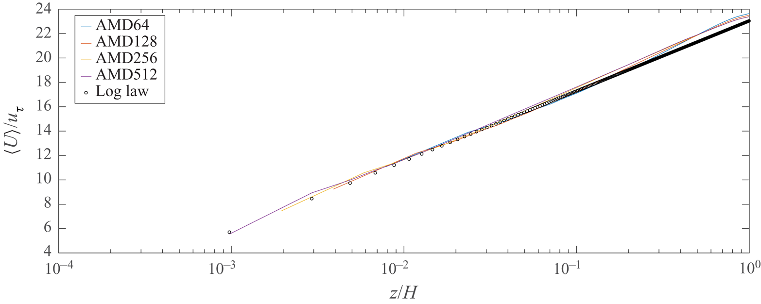
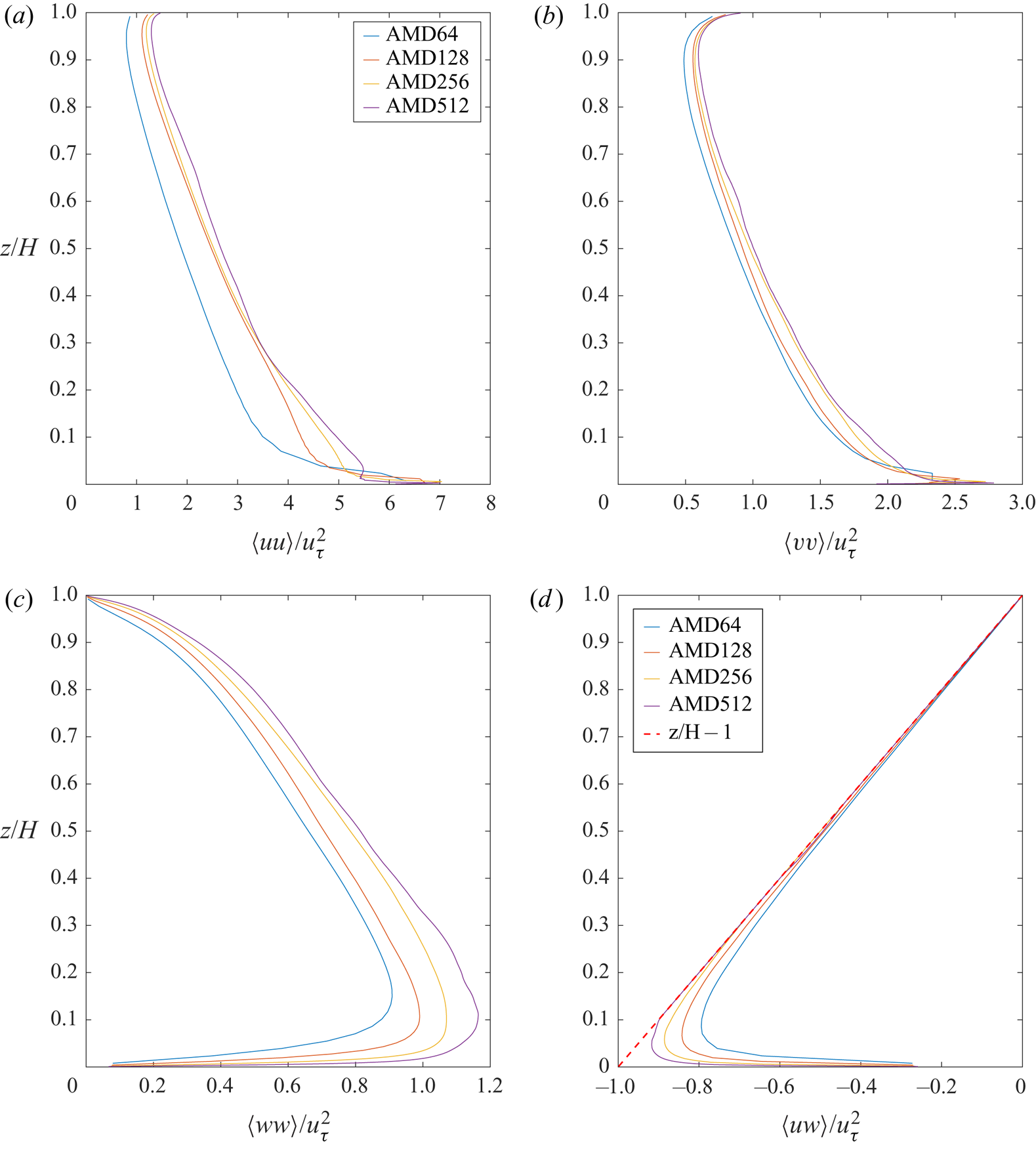
Figures 19 and 20 show mean velocity and Reynolds stresses for the coarse LES simulations at varying resolutions. While the mean velocity profiles clearly demonstrate lack of any log-layer mismatch at all resolutions, the streamwise velocity variances near the walls for coarse grids are larger than the values obtained using the high resolution simulations, which is contradictory to the notion of filtering. Some physical insight into these persistent overpredictions was recently proposed by Bae et al. (Reference Bae, Lozano-Duran, Bose and Moin2018) who argue that the no-penetration boundary condition implicit in the equilibrium wall model used in our simulations, results in non-physical splatting of the resolved large scales. They report up to  $90\,\%$ overprediction of the streamwise variance in their
 $Re_\tau =2000$ simulations using a no-slip boundary condition. While the spanwise and vertical velocity variances are smaller in the coarse LES than the high resolution LES, we will show later (using IDEAL64) that these variances are still larger than the expected values at the
 $192\times 192\times 64$ resolution. While these errors are not unexpected (the present results are entirely consistent with the profiles shown in Porté-Agel, Meneveau & Parlange (Reference Porté-Agel, Meneveau and Parlange2000) for similar resolutions), it is clear that the AMD model (also true for the Sigma SGS model) overestimates all four pertinent single-point correlations at the coarsest resolution, especially in the near-wall region (
 $z<0.1H$). A second striking feature seen in the variance profiles is the significant underprediction of the streamwise variance
 $z>0.25H$ by the
 $64$-point simulation. This is related to the underprediction of energy in the large streamwise coherent structure corresponding to
 $k_x L_x/(2{\rm \pi} ) \approx 2$ and
 $k_y L_y/(2{\rm \pi} ) \approx 4$ wavenumber and our numerical experiments using the Sigma SGS model and the wall-damped Smagorinsky model showed the same flaw. The grid refinement study suggests that as the LES Nyquist wavenumbers increase, this spanwise coherent structure becomes more energetic, especially as the coarsest mesh at
 $192\times 192 \times 64$ is refined to
 $384\times 384 \times 128$. This improvement can be seen in terms of single-point correlations in figure 20. This energetic large-scale structure necessitates the use of such a large domain size for periodic simulations. The inability of coarse simulations to capture the correct energy in these large spanwise structures also implies that the coarse simulations inaccurately predict the integral length scales. While the total cross-stress
 $\langle u^\prime w^\prime + \tau ^{SGS}_{13} \rangle$ is grid independent (since a constant pressure gradient is used to drive the flow), the grid invariance of mean profiles using the AMD model also implies that the total turbulent kinetic energy (TKE) production rate
 $\langle u^\prime w^\prime + \tau ^{SGS}_{13} \rangle ({\textrm {d} \langle U\rangle }/{\textrm {d} z})$ is correctly predicted in the coarse simulations.
Mean profile using the AMD model for grid sizes increasing from  $192\times 192 \times 64$ through
 $1536 \times 1536 \times 512$.

Single-point second-order correlations using the AMD model from grid sizes increasing from  $192\times 192 \times 64$ through
 $1536 \times 1536 \times 512$: (a)
 $\langle u^\prime u^\prime \rangle$; (b)
 $\langle v^\prime v^\prime \rangle$; (c)
 $\langle w^\prime w^\prime \rangle$; and (d)
 $\langle u^\prime w^\prime \rangle$.

5.2. Gabor mode enrichment of low resolution LES
The three model inputs that need to be specified to initiate the Gabor modes (see Ghate & Lele (Reference Ghate and Lele2017) for details) are the following.
(i) Minimum wavenumber
$k_{min}$ associated with the embedded Gabor modes. This parameter is a purely geometric parameter and depends on the size of the quasi-homogeneous regions defined. Since in the WMLES described above, no grid stretching is used in the vertical direction, this parameter is simply computed using the coarse LES cell width (filter width), and does not vary in the wall-normal direction. The maximum sampling wavenumber is simply set to ensure that the induced fields when resolved on a $1536 \times 1536 \times 512$ grid do not alias.(ii) Pre-distortion isotropic length scale measure,
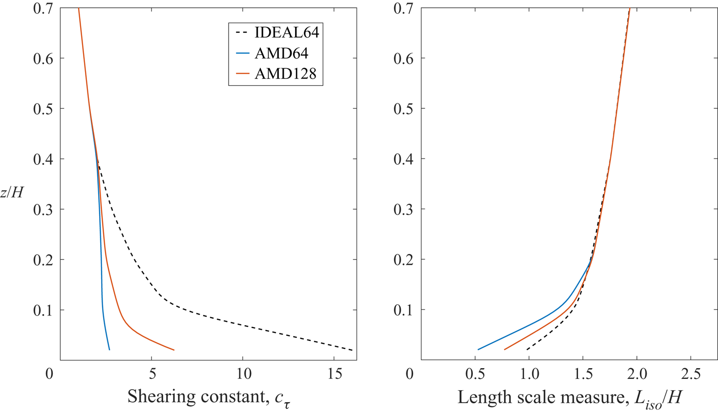
$L_{iso}$. Based on the discussion regarding inadequacy of coarse LES in predicting energy in the streamwise streaks, we use the following choice: $L_{iso}(z) = c_L\sqrt {L_x^v(z) L_y^v(z)}$, where the constant $c_L=1/0.67$ to ensure that in the limit of isotropy $L_{iso}$ is the integral length scale of isotropic turbulence. Note the preference of using spanwise velocity length scales over streamwise velocity length scales in order to reduce the influence of streamwise variance underprediction error in coarse LES on the enriched fields. For a stably stratified Ekman layer (as in Ghate & Lele Reference Ghate and Lele2017), the choice of streamwise velocity length scales was satisfactory because the stable stratification prevented the integral length scales from growing larger than boundary layer height. Our experience suggests that for a larger value of $L_{iso}$ (if $u$ length scales are used), implying larger $(k_{min}L_{iso})$, a larger shearing constant $c_\tau$ is needed in order to obtain the correct Reynolds stresses, thereby creating subfilter scales that are overly anisotropic.(iii) The shearing constant
$c_\tau$ which is computed by minimizing the least squares error in the Reynolds stress $\langle u^\prime w^\prime \rangle$ (see appendix B in Ghate & Lele Reference Ghate and Lele2017), which for this problem is a known analytical function of $z$.


Figure 21 shows the two inputs used for Gabor mode enrichment of the coarse simulation data. While all three coarse representations largely agree in the prediction of the length scale measure,  $L_{iso}$, it is clear that the shearing constant seen in AMD64 and AMD128 (to a lesser extent) is lower that what is expected from ideal filtering. This lower value of the shearing parameter results in enrichment of subfilter scales that are more isotropic than those expected by the implied grid filtering in coarser simulations for
 $z/H<0.2$, as is discussed in a subsequent section.
Model inputs for enrichment of the three coarse LES flow fields.

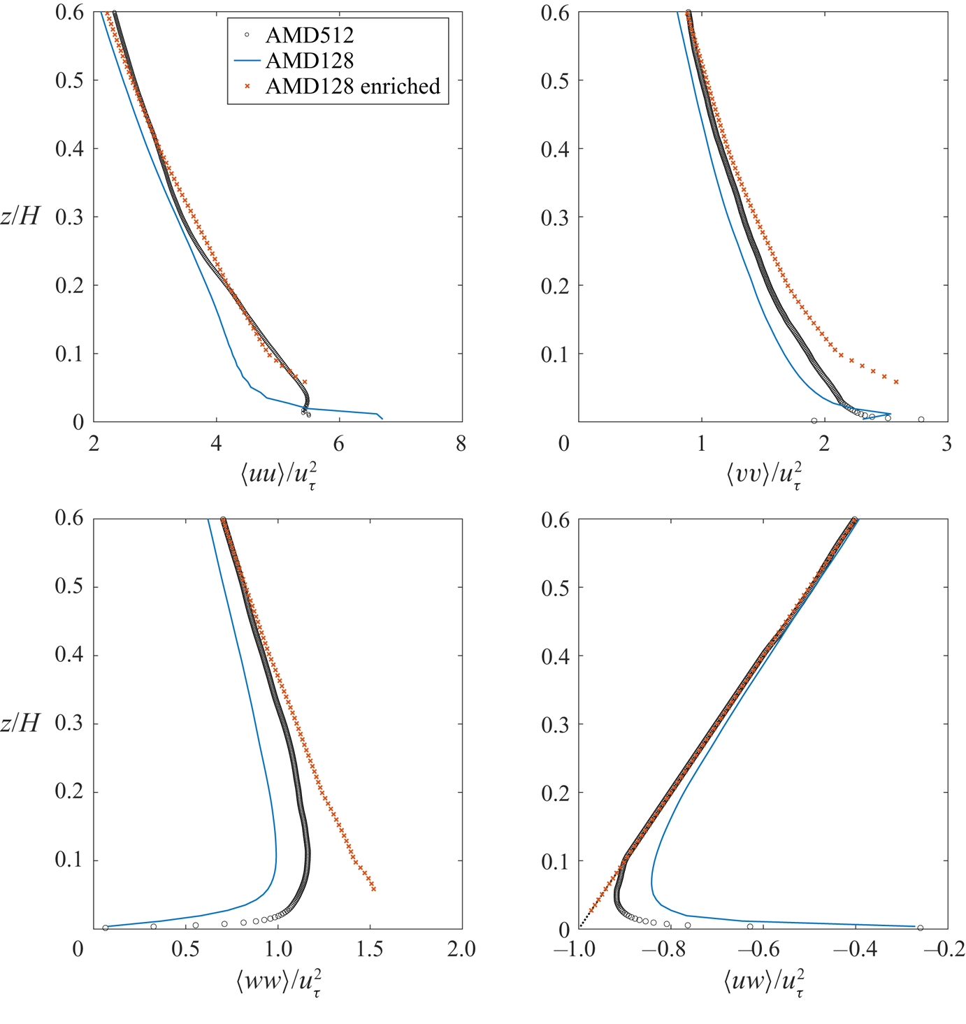
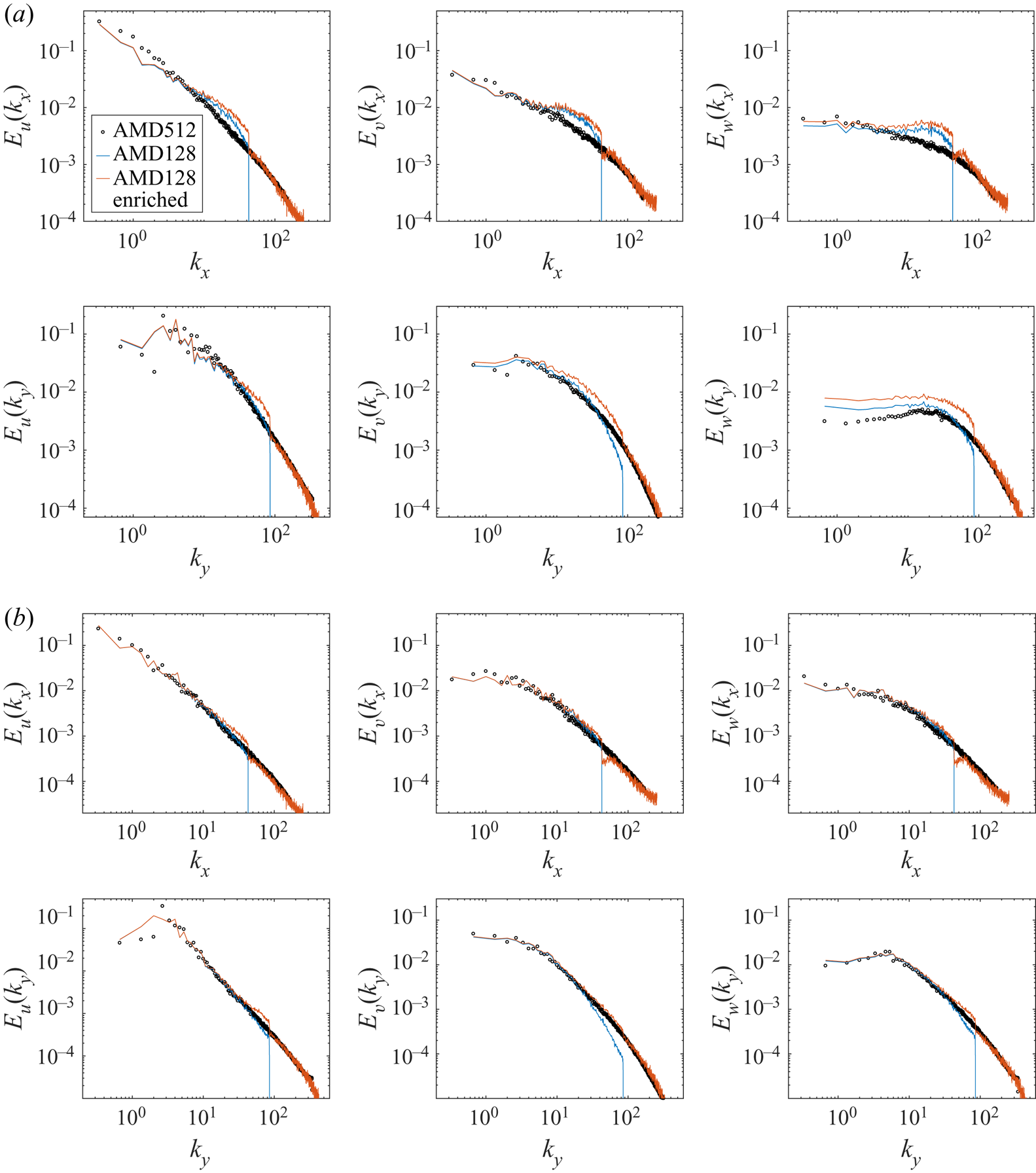
Figures 22 and 23 show the single-point and two-point (one-dimensional spectra) correlations for the Gabor mode enriched AMD128 case. The single-point correlations suggest that, for  $z/H>0.3$, the Gabor modes accurately represent the second-order statistics of the subfilter-scale turbulence. This is supported by the various one-dimensional spectra shown for all three components in figure 22(a) at
 $z/H=0.4$ where a consistent wavenumber extrapolation of each spectrum is observed. For
 $z/H<0.2$, while the single-point correlations show overprediction of variances, we note that the one-dimensional spectra suggest that this overprediction is primarily due to overprediction of the energy in low (resolved-scale) wavenumbers for the coarse simulation (see figure 22b). This is especially evident in the wall-normal velocity which appears to suffer from large aliasing at the
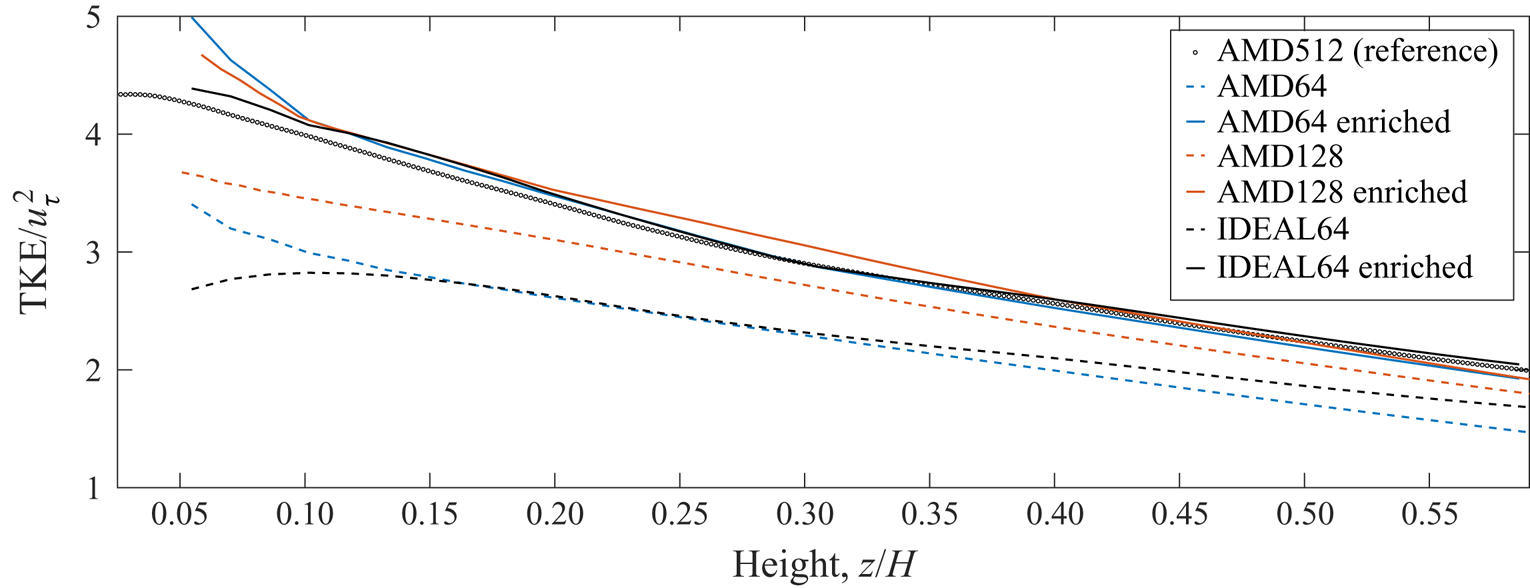
 $z=0.05H$ location. The turbulent kinetic energy profiles for both AMD128 and AMD64 are shown in figure 24. The figure shows that enrichment of both AMD128 and AMD64 recovers the total resolved turbulent kinetic energy of the reference simulation to a reasonable degree of accuracy at virtually all wall-normal locations. Furthermore, while some discrepancies exist between AMD64 and IDEAL64 for
 $z/H<0.15$, it is promising to note that the post-enrichment total TKE in the a posteriori setting (AMD SGS model) is similar to the TKE in the a priori setting (idealized filtering of reference simulation).
Single-point correlations as a function of height for the AMD128 case enriched using Gabor modes.

Velocity power spectra for Gabor mode enriched AMD128 LES: (a)  $z=0.40H$ and (b)
 $z=0.05H$.

Mean profiles of turbulent kinetic energy.

We now consider the single-point correlations for the AMD64 case in figure 25. The three variance profiles suggest that although the total subfilter TKE is reasonably accurate, the contributions of each of the three components has a qualitative bias at all wall-normal distances; the streamwise variance is underpredicted at the expense of substantial overprediction in the spanwise and wall-normal variances. In order to further explore this deficiency, we now consider the one-dimensional spectra for the three velocity components in figure 26. All size one-dimensional spectra considered at the two wall-normal locations indicate that virtually all the error in single-point correlations is a consequence of errors in the low-wavenumber region which is expected to be resolved by the coarse-grid LES. We will refer to this flaw observed in the 64-point simulations as over-enrichment and the following subsection discusses this aspect of a posteriori enrichment. Enrichment of the IDEAL64 case (shown in figures 27 and 28) is used to explain this over-enrichment in the a posteriori (AMD64) case.
Single-point correlations as a function of height for the AMD64 case enriched using Gabor modes.

Velocity power spectra for Gabor mode enriched AMD64 LES: (a)  $z=0.40H$ and (b)
 $z=0.054H$.

Single-point correlations as a function of height for the IDEAL64 case enriched using Gabor modes.

Velocity power spectra for Gabor mode enriched IDEAL64 LES: (a)  $z=0.40H$ and (b)
 $z=0.054H$.

5.3. Over-enrichment in coarse LES
The overall quality of the Gabor model enrichment for AMD64 can be broadly summarized using the following four observations.
(i) Significant underprediction of streamwise variances through the bulk of the boundary layer, particularly above
$z/H>0.1$. The one-dimensional spectra of $u$ at $z=0.4H$ (see figure 26b) confirm that this is entirely due to missing energy in the $k_x L_x/(2{\rm \pi} ) \approx 2$ and $k_y L_y/(2{\rm \pi} ) \approx 4$ coherent streak that was briefly discussed earlier. Since the present application is a one-way-coupled enrichment, Gabor mode enrichment simply cannot alleviate this deficiency of coarse simulations because it pertains to large wavelength meandering motions. For the IDEAL64 case, the filtering procedure does not remove any energy from this large streamwise coherent structure and as a result Gabor mode enrichment performs remarkably well as shown in figures 27 and 28. In other words, the profiles of the resolved Reynolds stress $\langle u^\prime w^\prime \rangle$ for AMD64 suggest that, for $z>0.2H$, the subfilter scales are primarily isotropic. However, the profiles for the streamwise velocity variances are inconsistent with this characterization of subfilter scales primarily due to the underprediction of the single-point correlation $\langle u^\prime u^\prime \rangle$ associated with the large coherent streak.(ii) The low dissipation property of the AMD model results in substantially more energy at barely resolved scales near its Nyquist limit, which is suggestive of aliasing. This is particularly evident in the
$k_y$ spectrum of spanwise and wall-normal velocity fluctuations, and also results in substantial overprediction of the Reynolds stress $\langle u^\prime w^\prime \rangle$. This results in an over-enrichment of the wall-normal velocity component when the variance of the enriched field is compared with the higher resolution simulation. This is in contrast to our observations for simulations done using the wall-damped Smagorinsky model (discussed in Ghate Reference Ghate2018) which is overly dissipative near the wall and consequently underpredicts the Reynolds stress, which results in Gabor mode enrichment of highly anisotropic small scales (seen in terms of large $c_\tau$ value) near the wall.(iii) The turbulent kinetic energy spectra at
$z/H=0.05$ and $z/H=0.40$ are shown in figure 29. Following figure 29, we note that the gradual decay in energy for values around the cutoff wavenumber (Nyquist wavenumber for coarse simulations) is due to anisotropy of the grid resolution ($\textrm {d} x=2\,\textrm {d} y$) and not due to excessively dissipative numerics or SGS modelling. At the $z/H=0.05$ plane, the LES512 case shows a prominent $k^{-1}$ energy scaling at low wavenumbers suggestive of production scales. However, it is apparent that the transition from $k^{-1}$ to $k^{-5/3}$ is not quite well resolved, which suggests that perhaps the AMD512 LES used for reference is not sufficiently well resolved at $z/H=0.05$. The primary purpose of showing the TKE spectrum along with the one-dimensional velocity spectra is to emphasize that if we evaluate solution quality using the TKE and its scale distribution, Gabor mode enrichment seems to work rather well. This is consistent with the basic philosophy of eddy viscosity type SGS modelling which attempts to correctly model the TKE cascade, but is not necessarily designed for accuracy in representing the spectral anisotropy. These results make a strong case for future work towards improving SGS modelling to improve representation of anisotropic effects in very coarse simulations of wall-bounded turbulence.(iv) Figure 20(a) suggests that AMD128 does not suffer from severe underprediction of energy in the large spanwise coherent structure, like the
$192\times 192\times 64$ simulations. However, Figure 20(d) indicates that the increase in grid points does not remove the overprediction in Reynolds stress ($\langle u^\prime w^\prime \rangle$) near the wall; in fact, the resolved Reynolds stress also increases as the grid is refined from AMD64 to AMD128. It is clear that while overshoots in spanwise and vertical velocity variances still persist (over prediction of resolved Reynolds stress by AMD128 requires enriched scales to be more isotropic than true subfilter scales), the underprediction of single-point correlations for $z>0.2H$ is not present anymore. Further work is needed to study the failure of SGS models at predicting the correct resolved near-wall anisotropy in the asymptotic Reynolds number limit ($Re\to \infty$).





Turbulent kinetic energy spectrum using polar wavenumber,  $k_{2d} = \sqrt {k_x^2 + k_y^2}$: (a)
 $z=0.054H$ and (b)
 $z=0.40H$. The TKE spectrum has been defined (and normalized) such that
 $({\langle u_i u_i \rangle }/{2})(z) = \int _{0}^{\infty } E(k_{2d})\,\textrm {d} k_{2d}$.

Again, it is important to emphasize that while the single-point correlation profiles in figure 25 suggest limited success in Gabor mode enrichment of the flow studied in this section, the analysis using one-dimensional spectra suggests otherwise. Even though the two-point statistics of the large scales predicted using the three SGS models have some deficiencies, the enrichment procedure does embed small scales that are fairly representative of the true subfilter scales. Much of this is attributed to informed choice of using an input length scale ( $L_{iso}$) measure computed using spanwise velocity fluctuations instead of streamwise fluctuations.
6. Conclusions
The turbulence enrichment approach using spatially and spectrally localized Gabor modes introduced by Ghate & Lele (Reference Ghate and Lele2017) is significantly developed and extended in this work. We formally define the turbulence enrichment problem to be the one where subfilter scales are superposed on large scales resolved on coarse-grid LES where the subfilter scales exhibit the following properties: (a) consistent extrapolation of second-order spectra and two-point spatial correlations for spatially inhomogeneous turbulence; (b) representation of spatially localized and intermittent interscale energy transfer from large to small scales; and (c) accurate characterization of physics responsible for temporal decorrelation of the enriched scales. Under an assumption of local quasi-homogeneity of near-filter scales, Gabor wavepackets/modes provide an optimal basis for representation of solenoidal velocity scales that can represent a physically consistent and realizable structural anisotropy. They enable significant compression in degrees of freedom needed for representation of subfilter-scale turbulence. Furthermore, by using WKB arguments, the temporal evolution of these small scales is expressed via simple ordinary differential equations for each Gabor mode. The rendering algorithm (see appendix B) shows that the velocity fields can be computed in physical space on finer numerical grids using an efficient non-uniform fast Fourier transform. Rendering can either be done at point locations or a subset of the physical domain without having to evaluate the fields in the entire domain at each simulation time step. This computational efficiency of the algorithm can facilitate its use in applications beyond LES enrichment such as inflow generation as was done recently in Ghate, Towne & Lele (Reference Ghate, Towne and Lele2020).
We investigate the accuracy of the enrichment algorithm for two LES problems in an a posteriori setting. In the first problem forced homogeneous isotropic turbulence is studied and the analysis shows that the enrichment not only provides an accurate scale-space extrapolation of the coarse LES, but also captures the interscale transfer of energy very accurately. The small scales represented by Gabor modes can be interpreted as velocities induced by a set of Burgers–Townsend vortices dispersed within quasi-homogeneous regions with their orientations defined by the gradients of the larger scales. The second problem considers a rough-wall boundary layer at large Reynolds number in a half-channel configuration. Two deficiencies relating to aliasing of vertical velocity (near walls) and the underprediction of energy in large streamwise structures by coarse-grid LES using conventional SGS models are identified. Despite these deficiencies of the original LES model, the enrichment leads to promising results, especially when enrichment is characterized by the increase in turbulent kinetic energy. We argue that accurate differentiation of physical anisotropy associated by Reynolds stress transport and the geometric anisotropy associated with the grid filtering is needed by the enrichment algorithm in order to provide correct variances for the enriched fields. Future development of this enrichment approach will focus on applications to non-equilibrium flows, analysis of subfilter-scale enriched pressure and analysis of higher-order moments implied in the enrichment.
Acknowledgements
A.S.G. was funded by Tomkat Center for Sustainable Energy at Stanford University. S.K.L. acknowledges partial support from NSF-CBET-1803378. All simulations were performed on Stampede2 supercomputer under the XSEDE project ATM170028. The authors would also like to thank the anonymous referees for their thoughtful comments and contribution to this work.
Declaration of interests
The authors report no conflict of interest.
Appendix A. Choice of scale-separation parameter $\varepsilon$ and error in divergence

One of the consequences of velocity field evaluation using (3.8) is that the synthesized velocity field is not exactly divergence free since the gradient of the cosine support function is not orthogonal to the induced velocity vector. It is easy to see that the true divergence is  $ {O}(\varepsilon )$, which provides an interesting opportunity to study the impact of the scale-separation parameter,
 $\varepsilon$. However, note that the velocity field synthesized can in fact be projected onto an exact divergence free basis at negligible extra computational cost, since we can simply project each of the contributions in (3.8) individually/locally using fast Fourier transforms in the support region (regardless of the global boundary conditions), thereby replacing (3.8) with
 \begin{align} \boldsymbol{u}(\boldsymbol{x}) = \sum_{i = 1}^{N_b} \boldsymbol{u}^\perp(\boldsymbol{x},\boldsymbol{x}_0^{(i)});\quad \boldsymbol{u}^\perp (\boldsymbol{x},\boldsymbol{x}_0^{(i)}) = \texttt{ifft}\left\lbrace \left(\delta_{ij} - \frac{K_i K_j}{K_m K_m} \right) \cdot \texttt{fft}\lbrace \boldsymbol{u}(\boldsymbol{x},\boldsymbol{x}_0^{(i)})\rbrace \right\rbrace, \end{align}
where the upper case  $K_i$ is used to denote equispaced wavenumbers corresponding to the support of the quasi-homogeneous region. (In practice one needs to deal with the odd-ball wavenumber before using the projection in (A 1).) Figures 30 and 31 show the impact of this exact divergence projection on the induced field, for example, synthesis of isotropic turbulence for two choices of the scale-separation parameter,
 $\varepsilon$, taken as 0.25 and 0.0625. The
 $\varepsilon = 0.25$ case corresponds to enrichment used throughout this paper, while the
 $\varepsilon = 0.0625$ case is generated by setting
 $(\varDelta _{QHx},\varDelta _{QHy},\varDelta _{QHz}) = (8\varDelta _x, 8\varDelta _y, 8\varDelta _z)$. In practice this is interpreted as the resolution of LES increased by a factor of 4 in each direction. These results show that a reduction of
 $\varepsilon$ by a factor of 4 results in reduction in divergence error. Furthermore, the loss in KE due to production is essentially negligible. However, recall that this reduction in
 $\varepsilon$ comes at a loss of spatial localization since the support function is four times as wide as the theoretical minimum. The comparison of the energy spectra further shows that the impact of this exact projection (A 1) is rather negligible in terms of the overall energy even for the
 $\varepsilon =0.25$ case. Comparison of two-point correlations between the two fields also suggests negligible impact of the local projection. This is an excellent prospect since it suggests that we can avoid the additional projection and thereby evaluate the fields directly at the required location as opposed to evaluating them on a Cartesian mesh,
 $\boldsymbol {x}$. For example, for an application involving arbitrary located particles at
 $\boldsymbol {x}_p$, the sum in (3.8) can again be computed using a type III NUFFT if a direct evaluation is prohibitively expensive.


Appendix B. Fast rendering algorithm using non-uniform FFTs
The overall algorithm discussed in this appendix relies on the Gabor mode description shown in figure 4. This illustration leads to the following three key observations: (a) the Gabor modes within each quasi-homogeneous region affect the flow within the quasi-homogeneous region, and a portion of the immediately adjacent quasi-homogeneous regions; (b) the velocity field at each location in physical space is a superposition of contributions from eight quasi-homogeneous regions in three-dimensional space; and (c) the Gabor modes advect in time similar to passive tracers, or non-inertial particles. This means at two different times the set of modes in a specific QH region changes with time.
B.1. Hybrid MPI+X rendering
Since most modern computational many-core architectures strongly favour an MPI+X paradigm, we first identify the tasks necessary in an MPI formulation (single program, multiple data).
(i) Mode transfer: latency bound, can be done using non-blocking, point-to-point communicators.
(ii) Gabor transform: bandwidth bound, can be done using non-blocking, point-to-point communicators.
Further note that the implementation of the purely MPI code is trivial and requires the use of halo-region exchanges (accomplished here using non-blocking point-to-point communicators) and particle/mode exchanges also requiring non-blocking point-to-point communicators. However, the halo-cell exchanges (physical space induced velocities) are a substantial bottle neck since each overlap in the region of influence consists of around 8–16 points (along each direction). This communication cost scales linearly with the surface area of processor decompositions. Therefore, there appears to be a substantial advantage of reducing the total number of MPI processes spawned during execution, and, hence, the choice to pursue a hybrid MPI  $+$ OpenMP implementation was made. The shared memory aspect of the parallelization (OpenMP) requires substantial modifications to a serial implementation of the enrichment algorithm due to the multitude of race conditions that occur in both the Gabor transform, and the particle evolution phases. Hence, the focus of the rest of this appendix will be limited to this shared memory portion of this implementation. The distributed memory aspects are identical to solutions to PDEs using finite difference schemes; i.e. it requires neighbour halo-exchanges for the Eulerian data, as well as neighbour point-to-point communications for any Gabor mode exchanges. All MPI calls are made by a single thread (the OMP SINGLE directive is used to identify the thread).
B.2. The overall enrichment algorithm
The overall shared memory algorithm can be decomposed into the following set of steps.
(i) Initialization/seeding of random modes in each QH region. This is done by simply distributing the QH regions among threads for the portion of the domain represented by each MPI process. Thread and process independent seeds are used to ensure reproducibility of the stochastic initialization.
(ii) Rendering (transform from Gabor modes to physical space fields). This is performed by modifying the Greengard & Lee (Reference Greengard and Lee2004) non-uniform fast Fourier transform algorithm.
(iii) Particle evolution. Since the particles within each QH region evolve due to the large-scale gradients within that QH region, this portion of the particle evolution is trivial to perform using multiple threads. However, the particles also advect to regions outside their original QH regions, and, hence, require to be resorted/histrogramming. While this process can be performed using multiple threads, special attention is needed to avoid the ensuing race conditions.
B.3. Gabor transform/rendering using OpenMP
The Gabor transform from a set of  $m$ modes to the uniform mesh in physical space can be expressed as two successive steps.
(i) Gaussian gridding (convolution): this step is operationally
$ {O}(m)$.(ii) Three-dimensional fast Fourier transform: this step is operationally
$ {O}(\tilde {N}^3\log _2(\tilde {N}))$, where $\tilde {N}$ is an upsampled mesh depending on the desired precision. For present applications, $10^{-9}$ precision requires twice upsampling and as such this FFT operation is approximately eight times as expensive as a regular FFT. That is, the FFT portion of an NUFFT to $N$ grid points has an operational complexity of $ {O}(8N^3\log _2(N))$.


Since each grid point is influenced by Gabor modes in eight QH regions, the NUFFT cannot be performed simultaneously in adjacent QH regions due to the implied race conditions. To overcome this limitation (and to speed up the NUFFT) a further decomposition is made in wavespace  $k$ for each QH region (see figure 32). Since the contribution due to large
 $k$ values requires a high resolution mesh, we cannot compute and store the field generated by each QH region in a temporary buffer (one buffer for each QH region would require a memory eight times larger than the problem size since window support is a factor of 2 larger than QH region in each direction). However, we again leverage the logarithmic sampling in
 $k$-space as shown in figure 32. The calculation of the NUFFT is now performed in three stages.
(i) The NUFFT from the low
$k$ modes is evaluated on a coarse mesh spanning the entire region of influence (RoI or support of the window), this operation typically uses about $85\,\%$ of the modes within the QH region. This data can be represented on a coarser mesh (see figures 33a and 33b, bottom pane), so it is stored in memory for each QH region separately. This operation uses a single NUFFT call.(ii) The RoI surrounding a QH region is decomposed into
$4\times 4\times 4$ subdomains (QH region into $2\times 2 \times 2$ octants), and the transform from large $k$ to each one of these octants is computed recursively. There are two algorithms implemented for this transform: (a) naive NUFFT (figure 33a) and (b) partial NUFFT (figure 33b). Depending on the application and the CPU architecture, the partial NUFFT algorithm can be 4–5 times faster than the naive algorithm due to substantially higher arithmetic intensity and the use of level 2 BLAS call (DGEMV/SGEMV). The data from the coarse grid (step 1), low $k$ mode is oversampled within each octant sequentially. The resulting race conditions between threads are prevented by using $4\times 4 \times 4$ OpenMP barrier calls. Finally, note that at this stage the code does not perform any interpolation from step 1 data; instead it simply stores the higher resolution grid data obtained at the end of the NUFFT since the NUFFT call anyway uses a twice upsampled grid for the FFT. As a consequence it requires at least eight times more memory than the number of degrees of freedoms; future implementations can address this by performing explicit interpolation using cubic splines.


Prep stage: the modes in each QH region are decomposed into large shells and small shells based on a cutoff wavenumber,  $k_{abs}$. In our application this decomposition ratio results in approximately
 $7{:}1$ in number of modes in each category. If
 $m$ modes are present, this operation does NOT require a sorting operation; instead it is performed using
 $m$ conditional statements and copies and as such the complexity is
 $ {O}(m)$ which is lower than that of quicksort.

Compute stage: each subset of Gabor modes is transformed separately on a different set of physical grids. This is done in order to reduce race conditions in the OpenMP portion of the calculations, and also for improved efficiency (in case of the partial NUFFT algorithm). (a) Naive NUFFT algorithm and (b) partial NUFFT algorithm.

Finally, note that for the compression ratios typically seen in applications ( ${>}85$) the cost is almost entirely given by the FFT stage of the NUFFT performed in step 2. The cost of step 1 is approximately a factor of 6–8 times smaller than that of step 2. Now since the NUFFT in step 2 is performed on a twice oversampled mesh, our numerical experiments show that the cost of NUFFT using
 $m$ modes on
 $N$ grid points is approximately 10 times larger than the cost of computing a single three-dimensional FFT on
 $N$ grid points for
 $m \ll N$.
B.4. Computational cost of the overall algorithm
Finally, let us return to the HIT enrichment example to illustrate the overall operational count of the enrichment algorithm. We will consider the HIT enrichment example studied in § 5.1.
(i) LES problem size,
$N_\texttt {LES} = 32^3$.(ii) Number of quasi-homogeneous regions,
$N_\texttt {QH} = 16^3$.(iii) Number of Gabor modes per QH region,
$m = 512$.(iv) Number of grid points to represent the enriched fields,
$N = 256^3$.(v) Compression in degree of freedom:
$(1 - {N_\texttt {QH}\times m}/{N}) \times 100 = 15\,\%$ (can do better by reducing $m$ or increasing $N$).(vi) Number of grid points within RoI for each QH region,
$N_\texttt {RoI} = 2^3 ({N}/{N_\texttt {QH}}) = 32^3$, since RoI is twice as wide as the QH region.(vii) Total number of NUFFTs needed:
$N_\texttt {QH} = 16^3$.(viii) Cost per NUFFT:
(a) naive NUFFT algorithm: cost per transform is
$ {O} (\lambda N_\texttt {RoI}\log _2 (N_\texttt {RoI}^{1/3}))$, where $\lambda$ is the ratio of cost of FFT to cost of NUFFT and is approximately $10$ for the present application where $m/N_\texttt {RoI} = 0.0156$. Total cost of transforming each field from Gabor modes to the entire domain: $(\lambda N_{QH}) \times {O} ( N_\texttt {RoI}\log _2 (N_\texttt {RoI}^{1/3}))$. This corresponds to $\lambda N_\texttt {QH}$ many $N_\texttt {RoI}$ sized three-dimensional FFTs.(b) partial NUFFT algorithm: cost per transform is
$ {O} (({\lambda }/{8}) N_\texttt {RoI}\log _2 (N_\texttt {RoI}^{1/3}) + mN_\texttt {RoI})$, where the first term is the NUFFT for coarse grid and the second term is a direct transform for the fine grid. Total cost of transforming each field from Gabor modes to the entire domain: $(({\lambda }/{8}) N_{QH}) \times {O} ( N_\texttt {RoI} (\log _2 (N_\texttt {RoI}^{1/3}) + {8m}/{\lambda }))$. Given $\lambda /8 \approx 1$ this cost can be interpreted primarily as $N_\texttt {QH}$ many $N_\texttt {RoI}$ sized three-dimensional FFTs, followed by $N_\texttt {RoI}$ many $m \times N_\texttt {QH}$ sized matrix vector products.


Operationally,  $\lambda$ depends on the choice of the library used for FFT portion of the NUFFT, and our numerical experiments suggest
 $\lambda \approx 11$ for FFTW and
 $\lambda \approx 9$ for fftpack. Using the naive NUFFT algorithm, the cost of a serial calculation of the Gabor mode velocities on a
 $256^3$ mesh is approximately equivalent to the cost of performing 35 three-dimensional FFTs of size
 $256^3$ using the FFTW library with AVX2 vectorization. Using the partial NUFFT algorithm, the cost of a serial calculation of the Gabor mode velocities on a
 $256^3$ mesh is approximately equivalent to the cost of performing 8 three-dimensional FFTs of size
 $256^3$ using the FFTW library with AVX2 vectorization.
Note that this calculation does not indicate the total cost of simulation using Gabor modes. The bulk of the cost reduction using Gabor modes lies in the temporal evolution description via a set of ordinary differential equations and as such this transform needs to be performed only when the fields need to be evaluated in physical space. Furthermore, the algorithm allows for the transform to be performed locally; only physical regions of the domain that need finer scale information need to use the transform.
In this worst case scenario, where the subfilter scales are needed in the entire domain at each small-scale time step, this factor of  $35$ for the cost of a single transform from Gabor modes to physical space is still substantially smaller than evaluation of the full equations using conventional methods, where just an iterative Poisson solver typically requires
 $ {O}(1000N)$ operations per time step (assuming Runge–Kutta substeps) for incompressible flow evaluations.
Appendix C. Temporal evolution equation for a Gabor mode
In order to derive the Gabor mode evolution equation we make the following arguments regarding the superfilter fields. Given a quasi-homogeneous region,  $x \in \mathcal {D}(\boldsymbol {x}_0)$ and a corresponding time scale,
 $\tau$:
(i) the superfilter field
$U_i(x_i)$ is expanded in space as
(C 1)\begin{equation} U_i (x_i) = U_i ^0 + x_j \left. \partial_j U_i \right|^0,\quad x \in \mathcal{D}(\boldsymbol{x}_0); \end{equation}(ii) the Galilean transform to the sweeping frame
(C 2)\begin{equation} \tilde{x}_i = x_i - U_i^0 t,\quad t \in [0, \tau]. \end{equation}


Consider the evolution of subfilter scales (2.8a,b) in the sweeping frame,
 \begin{equation} \partial_t u_i + (x_m \partial_m U_j) \partial_j u_i = -u_j \partial_j U_i -\partial_i p + \partial_j h_{ij} + \frac{1}{{Re}} \partial_j \partial_j u_i + \partial_j \tau_{ij}, \end{equation}
where  $h_{ij}$ is the stress associated with non-local (quadratic) interactions,
 $h_{ij} = -(u_i u_j + U^r_i u_j + u_i U^r_j)$. Next, by assuming Gabor modes of the form for an arbitrary function,
 $f(\boldsymbol {x},t)$,
 \begin{equation} f(\boldsymbol{x},t) = \sum \hat{f}(\boldsymbol{x}_0,t, \varepsilon) \exp({\textrm{i}(\boldsymbol{k}(t)\cdot\boldsymbol{x})}), \end{equation}
where the  $\hat {f}(\boldsymbol {x}_0,t)$ is the complex amplitude (
 $\boldsymbol {x}_0$ is a coordinate fixed with the large scales;
 $\textrm {d}\boldsymbol {x}_0/\textrm {d} t = U(\boldsymbol {x}_0)$) with the spatial windowing corresponding to a scale-separation ratio,
 $\varepsilon$. Thus, for an arbitrary function, we have
 \begin{equation} \partial_j\,f(\boldsymbol{x},t) = \sum (ik_j(t) \hat{f}(\boldsymbol{x}_0,t,\varepsilon)) \exp({\textrm{i}(\boldsymbol{k}(t)\cdot\boldsymbol{x})}) + {O}(\varepsilon). \end{equation}
We will use this identity to substitute the modes (C 4) into the governing equation for small scales (C 3). However, we will first derive the eikonal equation which describes the temporal evolution of wavenumbers,  $\boldsymbol {k}(t)$. Consider an arbitrary (passive) scalar field
 $\phi (\boldsymbol {x},t)$ advected by the large-scale field
 $\boldsymbol {U}(\boldsymbol {x},t)$. That is, the scalar field
 $\phi (\boldsymbol {x},t)$ satisfies
 \begin{equation} \frac{\textrm{D}\phi}{\textrm{D} t} = \partial_t \phi + U_j \partial_j \phi = 0. \end{equation}
Now, assuming a modal representation of the field at time  $t=0$ of the form
 \begin{equation} \phi(\boldsymbol{x},t=0) = \hat{\phi}(\boldsymbol{x}_0, \varepsilon) \exp({\textrm{i}\boldsymbol{k}\boldsymbol{\cdot} \boldsymbol{x}}), \end{equation}
the eikonal equation can be obtained by postulating that the temporal evolution of the field  $\phi (\boldsymbol {x},t)$ can be obtained by a constant (in time) amplitude
 $\hat {\phi }$ (in the frame of
 $\boldsymbol {x}_0$) and time dependent wavenumber
 $\boldsymbol {k}(t)$. Simple substitution of (C 7) into (C 6) and using the properties
 $U_i(\boldsymbol {x},t) = U_i(\boldsymbol {x}=0) + \partial _j U_i (x_j - x^0_j)$ (quasi-homogeneity) and the definition
 $\textrm {d}\boldsymbol {x}_0/\textrm {d} t = \boldsymbol {U}(\boldsymbol {x}_0)$, we get
 \begin{equation} \frac{\textrm{D} \phi}{\textrm{D} t} = \textrm{i} \hat{\phi}(\boldsymbol{x}_0) x_j \left(\frac{\textrm{d} k_j}{\textrm{d} t} + k_m \frac{\partial U_m}{\partial x_j} \right) = 0. \end{equation}
Due to the arbitrary nature of  $\phi$, we now have the eikonal equation for
 $\boldsymbol {k}(t)$:
 \begin{equation} \partial_t k_j + k_m \partial_j U_m = 0. \end{equation}
Using this evolution equation for the wavenumbers, we can show that the Gabor mode representation of the left-hand side of (C 3) is given as
 \begin{equation} \partial_t u_i + (x_m \partial_m U_j) \partial_j u_i = \exp({\textrm{i}\boldsymbol{k}(t)\cdot\boldsymbol{x}}) \partial_t \hat{\boldsymbol{u}}(\boldsymbol{x}_0, t, \varepsilon) + {O}(\varepsilon). \end{equation}
Now consider the straining terms that appear on the right-hand side of (C 3). The Gabor mode representation of the straining terms (using quasi-homogeneneity assumptions) is simply
 \begin{equation} \widehat{u_j \partial_j U_i} = \hat{u}_j(\boldsymbol{x}_0, t, \varepsilon) \partial_j U_i(\boldsymbol{x}_0,t). \end{equation}
Substituting these definitions in (C 3), we get
 \begin{equation} \partial_t \hat{u}_i = -\hat{u}_j \partial_j U_i - \textrm{i}k_i\hat{p} + \textrm{i}k_j \hat{h}_{ij} + \frac{1}{{Re}} \partial_j \partial_j \hat{u}_i + \textrm{i}k_j \hat{\tau}_{ij}. \end{equation}
The pressure term can be eliminated by multiplying (C 12) by the projection tensor  $(\delta _{im} - {k_i k_m}/{k_l k_l} )$ and noting that
 \begin{equation} \left(\delta_{im} - \frac{k_i k_m}{k_l k_l} \right)(\textrm{i} k_i \hat{p}) = \textrm{i} k_m\hat{p} - \textrm{i} k_m \hat{p} = 0. \end{equation}
Upon projection (and using the property  $k_m \hat {u}_m = {O}(\varepsilon )$), the left-hand side of (C 12) simplifies to
 \begin{equation} \partial_t \hat{u}_m - \frac{k_i k_m}{k_l k_l}\partial_t \hat{u}_i = \partial_t \hat{u}_m - \left(- \frac{\hat{u}_i}{k_l k_l}\partial_t(k_i k_m) \right) + {O}(\varepsilon)= \partial_t \hat{u}_m - \left(- \frac{k_m \hat{u}_i}{k_l k_l}\partial_t(k_i) \right) + {O}(\varepsilon). \end{equation}
Now using the eikonal equation (C 9), we get
 \begin{equation} \left(\delta_{im} - \frac{k_i k_m}{k_l k_l} \right)\partial_t \hat{u}_i = \partial_t \hat{u}_m - \left(\frac{k_m k_p}{k_l k_l}\right) \left(\hat{u}_i \partial_i U_p\right) + {O}(\varepsilon). \end{equation}
Similarly, the straining term projects as
 \begin{equation} \left(\delta_{im} - \frac{k_i k_m}{k_l k_l} \right) \left(-\hat{u}_j \partial_j U_i\right) = -\hat{u}_j \partial_j U_m + \left(\frac{k_m k_i}{k_l k_l}\right) \left(\hat{u}_j \partial_j U_i\right). \end{equation}
Substituting (C 15) and (C 16) into (C 12), we get
 \begin{equation} \partial_t \hat{u}_m = -\hat{u}_k \partial_k U_j \left(\delta_{mj} - 2\frac{k_m k_j}{k_l k_l} \right) + \textrm{i}k_j \hat{h}^{\perp}_{mj} + \frac{1}{{Re}} \partial_j \partial_j \hat{u}_m + \textrm{i}k_j \hat{\tau}^{\perp}_{mj} + {O}(\varepsilon), \end{equation}
where  $\hat {h}^{\perp }_{ij} = (\delta _{im} - {k_i k_m}/{k_l k_l}) \hat {h}_{mj}$ and
 $\hat {\tau }^{\perp }_{ij} = (\delta _{im} - {k_i k_m}/{k_l k_l} ) \hat {\tau }_{mj}$.