1. Introduction
In recent decades, the mortality of most developed countries was gradually declining as a result of improvements in public health, medical advances, lifestyle changes and government regulation. Although it is an obvious benefit for society, this longevity improvement could also represent a risk for governments and insurance companies. Indeed, if they do not properly consider these improvements in retirement planning and the life insurance products’ pricing, they could get in financial trouble. The risk that future mortality and life expectancy outcomes turn out different than expected is typically called longevity risk and, as pointed out in Barrieu et al. (Reference Barrieu, Bensusan, El Karoui, Hillairet, Loisel, Ravanelli and Salhi2012), its management requires stochastic mortality projection models. In this vein, a number of stochastic mortality models were developed.
One of the first stochastic models describing the mortality of a single population was proposed by Lee and Carter (LC) (Lee and Carter, Reference Lee and Carter1992). Their model decomposes the age-time matrix of mortality rates into a bilinear combination of age and period parameters using the principal component analysis (PCA), and forecasting is performed by projecting the time index component into the future with time-series models. A formal description of this model will be presented in the next section.
Numerous extensions of the LC model have been developed and proposed in the literature. For example, Brouhns et al. (Reference Brouhns, Denuit and Vermunt2002) embedded the LC model into a Poisson regression setting to overcome the homoskedastic error structure assumed into the original LC method. Renshaw and Haberman (Reference Renshaw and Haberman2003a) proposed a multi-factor version of the LC model to improve the goodness-of-fit, and a few years later (Renshaw and Haberman, Reference Renshaw and Haberman2006) generalised the Lee-Carter model including a cohort effect. Hyndman and Ullah (Reference Hyndman and Ullah2007) proposed a functional data approach in which the mortality curves are smoothed for each year using constrained regression splines prior to fitting a model using principal components decomposition and Hainaut and Denuit (Reference Hainaut and Denuit2020) further extended this method by using a wavelet-based decomposition.
Another very popular stochastic mortality model is the Cairns-Blake-Dowd model proposed in Cairns et al. (Reference Cairns, Blake and Dowd2006), and many of its extensions have been proposed. We refer to Cairns et al. (Reference Cairns, Blake, Dowd, Coughlan, Epstein, Ong and Balevich2009) for a review.
Since most of the drivers of the mortality improvements mentioned above often spread quickly, mortality changes over time between different countries appear, in some way, correlated. For this reason, the study of multi-population mortality models has received increasing attention within the mortality forecasting’ literature. Extensive use of these models is typical in reinsurance, and risk hedging (Enchev et al., Reference Enchev, Kleinow and Cairns2017; Villegas et al., Reference Villegas, Haberman, Kaishev and Millossovich2017). One of the simplest approaches for forecasting mortality of multiple populations consists of using Individual Lee-Carter (ILC) models (Li and Hardy, Reference Li and Hardy2011). In this case, the mortality of each population is described by an own LC model whose parameters are estimated separately from the other populations. This approach is relatively accurate and easy to implement even for a large number of populations; however, it completely ignores the dependency among mortality of the different populations. Some authors address this issue by introducing common terms in the individual models. A very popular model is the Augmented Common Factor model developed by Li and Lee (Reference Li and Lee2005) that proposes a double log-bilinear mortality model augmenting common age and period effects with sub–population-specific age and period effects. A second example is the Common Age Effect model proposed by Kleinow (Reference Kleinow2015). It assumes that only the age-specific LC parameters modulate the period effect are common to all populations, while different time indices fit each population. However, these models were usually intended for forecasting the mortality of similar populations and not for large-scale mortality forecasting. The comparative analysis in Richman and Wüthrich (Reference Richman and Wüthrich2021) highlights that these multi-population extensions did not perform fully competitively against the ILC approach when a large set of populations is considered.
Large-scale mortality forecasting is defined as the simultaneous production of forecasts for many different and potentially unrelated populations (Richman and Wüthrich, Reference Richman and Wüthrich2021). Examples of large-scale mortality forecasting tasks are forecasting the mortality rates of all the populations of the Human Mortality Database (HMD) or the United States Mortality Database simultaneously. Thanks to their ability to efficiently analyse large amounts of data; neural networks (NN) represent a natural candidate to address this challenge. Although NNs’ application to mortality modelling is quite recent, the scientific contributions are increasing in number and intensity. Hainaut (Reference Hainaut2018) proposed a NN approach to predict and simulate mortality rates of a single population. The author developed a neural analyser to extract latent time processes and directly predict mortality. This approach allows for detecting and replicating non-linearities observed in the evolution of log-forces of mortality. The same intuition motivated the contribution in Nigri et al. (Reference Nigri, Levantesi, Marino, Scognamiglio and Perla2019), in which the authors introduced Recurrent Neural Networks (RNNs) into the classical two-stage procedure of the LC approach. In particular, they employed Long Short-Term Memory (LSTM) networks to model the time-related index component. Furthermore, Lindholm and Palmborg (Reference Lindholm and Palmborg2021) explored the application of the LSTM networks in the Poisson LC model framework. Richman and Wüthrich (Reference Richman and Wüthrich2021) has the merit of developing the first large-scale mortality model based on NNs. They provided a NN architecture based on fully connected and embedding layers with notable forecasting accuracy. Perla et al. (Reference Perla, Richman, Scognamiglio and Wüthrich2021) further extended the model of Richman and Wüthrich (Reference Richman and Wüthrich2021) by introducing RNNs and convolutional neural networks (CNNs), specifically designed to model sequential data such as time-series data. The use of convolutional networks for mortality modelling was also investigated in Wang et al. (Reference Wang, Zhang and Zhu2020). Despite the models proposed in Richman and Wüthrich (Reference Richman and Wüthrich2021) and Perla et al. (Reference Perla, Richman, Scognamiglio and Wüthrich2021) present more accurate forecasts than the ILC approach, how to forecast uncertainty can be derived remains an open issue. This paper proposes a different approach to perform large-scale mortality forecasting. We use NNs for fitting some well-known mortality models without modifying their forecasting scheme. The main idea consists of developing neural network architectures that, on one side, replicate the model structure of the single-population mortality models and, at the same time, take into account and exploit the dependency among the mortality of different populations. To this purpose, we embed the individual LC models into a NN in which the classical LC parameters are jointly estimated by processing the mortality data of all populations simultaneously. Some authors have already discussed and pointed out that the estimates of LC age-specific parameters obtained with the traditional approaches sometimes present random fluctuations over the age dimension producing irregular projected life tables (Camarda and Basellini, Reference Camarda and Basellini2021). The most evident problems concern the estimates of the age-specific parameters modulating the period effect (denoted as
 $b_x$
in the original paper), and possible solutions were explored in the literature. Renshaw and Haberman (Reference Renshaw and Haberman2003b) proposed to smooth those estimates using parametric or non-parametric methods without modifying the other parameters. Alternatively, Delwarde et al. (Reference Delwarde, Denuit and Eilers2007) suggested imposing the smoothing within the estimation phase. The authors introduced a roughness penalty term in the least squares function (for the classical LC method) and log-likelihood function (for the Poisson LC model proposed in Brouhns et al., Reference Brouhns, Denuit and Vermunt2002) to encourage the smoothness of the parameters curve. The trade-off between goodness-of-fit and smoothness is controlled through a smoothing hyper-parameter that penalises the fluctuations. Currie (Reference Currie2013) further extend this approach imposing the smoothing of both age-related parameters (
 $a_x$
and
 $b_x$
). In that case, the objective function presents two penalty terms, and there are two hyper-parameters controlling the cost of the fluctuations in the two parameter’s curves, respectively. A successful application of these two methods requires a careful choice of the values of the smoothing hyper-parameters. According to the original papers, the selection of these values must be based on data, and the optimal values can be estimated by employing time-consuming cross-validation procedures. Using these two methods in a large-scale mortality forecasting context could be complex from a computational perspective since the cross-validation procedure for estimating the smoothing hyper-parameter should be applied individually to each population. We address this issue by proposing a parsimonious NN architecture specifically designed to calibrate each individual LC using all available information instead of using a population-specific subset of data as in the traditional estimation schemes. Some cross-population parameters encourage the information propagation among the individual model and produce estimates less sensitive to the random fluctuations often present in mortality rates’ data. Furthermore, the NN architectures developed present very few parameters to optimise and are easy to interpret. These features could encourage the use of NNs in mortality modelling also by practitioners who are wary of the use of complex and hard-to-interpret models even if they have high predictive power. Despite the simple structure of the NNs proposed, the forecasting performance is highly competitive with respect to other NN-based approaches proposed in the literature. The remainder of the paper is structured as follows: Section 2 provides a formal description of the LC model, Section 3 introduces the NN architectures employed in this paper, Section 4 formally presents the NN-based model, in Section 5 a large set of numerical experiments is illustrated, and finally, Section 6 concludes.
2. Lee-Carter model
The Lee-Carter (LC) model (Lee and Carter, Reference Lee and Carter1992) is an elegant and powerful approach to forecast a single population’s mortality. Let
 $\mathcal{X} = \{x_{0}, x_{1}, \dots, x_{\omega}\}$
be the set of the age categories and
 $\mathcal{T} = \{t_{0}, t_{1}, \dots, t_{n}\}$
be the set of calendar years considered. The LC model defines the logarithm of the central death rate
 $\log\!(m_{x,t}) \in \mathbb{R}$
at age
 $x \in \mathcal{X}$
in the calendar year
 $t\in \mathcal{T}$
as
 \begin{equation} \log\!(m_{x,t}) = a_x+b_x k_t+ e_{x,t},\end{equation}
where
 $a_x \in \mathbb{R}$
is the average age-specific pattern of mortality,
 $k_t\in \mathbb{R}$
is a time index that summarises the development in the level of mortality over time, and thus, it will capture the general time trend of the death rates,
 $b_x\in \mathbb{R}$
measures the loadings to the particular age groups when the mortality index changes and
 $e_{x,t} \in \mathbb{R}$
is the error term.
Since the model in (2.1) is over-parameterised, to avoid identifiability problems, the following constraints are imposed
 \begin{equation} \sum_{x \in \mathcal{X}} b_x = 1 \quad \quad \quad \sum_{t \in \mathcal{T}} \frac{k_t}{\mid \mathcal{T} \mid} = 0.\end{equation}
The ordinary least squared estimation of the model parameters in (2.1) can be obtained by solving the optimisation problem
 $$\mathop {{\rm{arg}}\,{\rm{min}}}\limits_{_{{{({a_x})}_x},{{({b_x})}_x},{{({k_t})}_t}}} \sum\limits_{x \in X} {\sum\limits_{t \in T} ( } \log ({m_{x,t}}) - {a_x} - {b_x}{k_t}{)^2}$$
The
 $(a_x)_x$
are estimated as the logarithm of the geometric mean of the crude mortality rates, averaged over all t, for each
 $x \in \mathcal{X}$
 \begin{equation*} \hat{a}_x = \log\!\left(\prod_{t\in \mathcal{T}} (m_{x,t})^{1/\mid \mathcal{T} \mid}\right),\end{equation*}
while
 $(k_t)_t$
and
 $(b_x)_x$
are estimated as the first right and first left singular vectors in the Singular Value Decomposition (SVD) of the centre log-mortality matrix
 $ M = \big(log(m_{x,t}) - \hat{a}_x \big)_{ x \in \mathcal{X}, t \in \mathcal{T}} \in \mathbb{R}^{|\mathcal{X}| \times |\mathcal{T}|}$
. In order to forecast, the parameters
 $(a_x)_x$
and
 $(b_x)_x$
are assumed to be constant over time while the time index
 $k_t$
is modelled as an ARIMA (0,1,0) process
 \begin{equation}k_t = k_{t-1}+ \gamma+ e_t \quad \quad with \ i.i.d \ e_t \sim N\left(0, \sigma_{\epsilon}^2\right),\end{equation}
where
 $\gamma \in \mathbb{R}$
is the drift.
A simple way of modelling the mortality of a set of different populations
 $\mathcal{I}$
is to describe each population separately with its own LC model
 \begin{equation} \log\left(m^{(i)}_{x,t}\right) = a^{(i)}_x+b^{(i)}_x k^{(i)}_t+ e^{(i)}_{x,t} \quad \quad \forall i \in \mathcal{I}.\end{equation}
This approach is sometimes called ILC approach. In this case, the model fitting is performed individually, and the population and time-specific terms
 $k_t^{(i)}$
are projected with independent ARIMA (0,1,0) processes. Although some multi-population extensions of the LC model are being proposed, the numerical study provided in Richman and Wüthrich (Reference Richman and Wüthrich2021) shows that these extensions produce good forecasting performance only in some cases and, the ILC approach remains highly competitive.
2.1. Poisson maximum likelihood estimation
The main drawback of SVD is the assumption of homoskedastic errors (Alho, Reference Alho2000). This issue is related to the fact that, for inference, we are actually assuming that the errors are normally distributed, which is quite unrealistic. Indeed, appear reasonable to believe that the logarithm of the observed log-mortality rates is much more variable at older ages than at younger ages because of the much smaller absolute number of deaths at older ones.
In Brouhns et al. (Reference Brouhns, Denuit and Vermunt2002), a maximum likelihood estimation based on a Poisson death count
 $D^{(i)}_{x,t}$
is proposed to allow heteroskedasticity. In this case, the ILC model for multiple populations reads
 \begin{equation}D^{(i)}_{x,t} \sim Poisson\!\left(E^{(i)}_{x,t} m^{(i)}_{x,t}\right) \quad with \quad m^{(i)}_{x,t} = e^{a^{(i)}_x + b^{(i)}_x k^{(i)}_t},\end{equation}
where
 $E^{(i)}_{x,t}$
is the number of exposure-to-risk in age x at time t in the population i and the constraints in (2.2) still hold for each population. The model parameters can be estimated by solving
 $$\mathop {{\rm{arg}}\,{\rm{max}}}\limits_{{{\left( {a_x^{(i)}} \right)}_x},{{\left( {b_x^{(i)}} \right)}_x},{{\left( {k_t^{(i)}} \right)}_t}} \sum\limits_{x \in {\cal X}} {\sum\limits_{t \in {\cal T}} ( } D_{x,t}^{(i)}\left( {a_x^{(i)} + b_x^{(i)}k_t^{(i)}} \right) - E_{x,t}^{(i)}{e^{a_x^{(i)} + b_x^{(i)}k_t^{(i)}}}) + {c_i},\quad \forall i \in {\cal I},$$
where
 $c_i \in \mathbb{R}$
is a constant which only depends on the data. The meaning of the parameters is essentially the same of the corresponding parameters in the classical LC model. Furthermore, in Brouhns et al. (Reference Brouhns, Denuit and Vermunt2002) the authors do not modify the time-series part of the LC method.
3. Feed-forward neural networks
Feed-forward NNs are popular methods in data science and machine learning. They can be considered high-dimensional non-linear regression models and achieve excellent performance in several fields. A feed-forward NN consists of a set of (non-linear) functions, called units, arranged in layers (input, output and hidden layers), which process and transform data to perform a specific task. How the units are connected configures different types of NNs. A brief description of the NN blocks used in the paper is provided below.
3.1. Fully connected neural networks
Fully connected networks (FCN) are probably the most popular type of feed-forward NNs. In FCN, each unit of a layer is connected to every part of the previous one. First, we describe a single FCN layer.
Let
 $\boldsymbol{y} = (y_1, y_2, \dots, y_{q_0})^\top\in {\mathbb R}^{q_0}$
be a
 $q_0$
-dimensional input vector, a FCN layer with
 $q_1\in{\mathbb N}$
hidden units is a function that maps the input
 $\boldsymbol{y}$
to a new
 $q_1$
-dimensional space
 \begin{equation} \boldsymbol{z}\;:\;\mathbb{R}^{q_0} \to \mathbb{R}^{q_1}, \quad \quad {\boldsymbol{y}} \mapsto \boldsymbol{z}({\boldsymbol{y}}) = \left( z_1({\boldsymbol{y}}), z_2 ({\boldsymbol{y}}), \dots , z_{q_1}({\boldsymbol{y}}) \right)^\top.\end{equation}
Each new feature component
 $z_j(\boldsymbol{x})$
is a non-linear function of
 $\boldsymbol{x}$
 \begin{equation}{\boldsymbol{y}}\; \mapsto \;\boldsymbol{z}_j({\boldsymbol{y}}) =\phi \left( w_{j,0} + \sum_{l = 1}^{q_0} w_{j,l} {y}_l \right) = \phi \left( w_{j,0} + \left\langle \boldsymbol{w}_j, {\boldsymbol{y}} \right\rangle \right), \quad \quad j = 1, \dots , q_1 ,\end{equation}
where
 $\phi \;:\; \mathbb{R} \to \mathbb{R}$
is a (non-linear) activation function,
 $w_{j,l} \in \mathbb{R}$
represent the network parameters and
 $\langle \cdot, \cdot \rangle$
denotes the scalar product in
 $\mathbb{R}^{q_0}$
.
When the FCN is shallow, it presents a single hidden layer followed by the output layer. Differently, a deep FCN provides several stacked FCN layers and the output of each layer becomes the input of the next one and so for the following layers. Let
 $\boldsymbol{q} = \{q_k\}_{1 \leq k \leq m} \in \mathbb{N}^{m}$
be a sequence of integers defining the size of each layer where
 $m \in \mathbb{N}$
is the number of hidden layers also called depth. A deep FCN can be formalised as:
 \begin{equation}{\boldsymbol{y}} \; \mapsto \; \boldsymbol{z}^{(m\;:\;1)} ({\boldsymbol{y}})=\left( \boldsymbol{z}^{(m)} \circ \cdots \circ \boldsymbol{z}^{(1)} \right) ({\boldsymbol{y}})\;\in \;{\mathbb R}^{q_m},\end{equation}
where all mappings
 $\boldsymbol{z}^{(k)}\;:\;\mathbb{R}^{q_{k-1}} \to \mathbb{R}^{q_{k}}$
adopt the structure in (3.1) with weights
 $W^{(k)} = \left(\boldsymbol{w}^{(k)}_j\right)_{1\leq j \leq q_k} \in {\mathbb R}^{q_k \times q_{k-1}}$
and biases
 $\boldsymbol{w}^{(k)}_0 \in {\mathbb R}^{q_k}$
, for
 $1 \leq k \leq m$
.
 $\phi_k$
are the activation functions of each layer which could also differ from each other.
Both shallow and deep FCNs include a final output layer that computes the variable of interest v as a function of the features extracted of the last hidden layer
 $\boldsymbol{z}^{(m\;:\;1)} ({\boldsymbol{y}})$
. This layer is a mapping
 $g\;:\;\mathbb{R}^{q_m} \to {\mathcal{V}} $
that must be chosen according to the domain of the response variable.
Given a specific prediction task, the performance of a deep FCN strongly depends on the weights
 $w^{(k)}_{j.l}$
that must be properly calibrated. Given a specific loss function
 $L(g(\boldsymbol{z}^{(m\;:\;1)} ({\boldsymbol{y}})),{v})$
, which measures the quality of the predictions produced by the network
 $g(\boldsymbol{z}^{(m\;:\;1)} ({\boldsymbol{y}}))$
against the observed values v of the response variable V, network training (or fitting) consists in finding the weights that minimise
 $L(g(\boldsymbol{z}^{(m\;:\;1)} ({\boldsymbol{y}})),{v})$
. It is generally performed via the Back-Propagation (BP) algorithm where the weights are updated iteratively to step-wise decrease the objective function, with each update of the weights based on the gradient of the loss function. An extensive description of network fitting and the BP algorithm is found in Goodfellow et al. (Reference Goodfellow, Bengio and Courville2016).
3.2. Locally connected neural networks
The traditional FCN layers do not consider the spatial structure of the data since they treat elements of the input data that are far or close to each other without distinction. The locally connected network (LCN) layers overcame this problem. They are characterised by the local connectivity since each unit of the layer is connected only with a local area of the input, called receptive field. The resulting weight matrices (called filters) present a smaller size than the input data, and the features extracted are functions of a small part of the input data. This induces a significant reduction of the parameters to optimise with respect to the traditional FCN layers. The feature map extracted by an LCN layer depends, among the other hyper-parameters, on the kernel filter’ size
 $m \in {\mathbb N}$
and the stride
 $s \in {\mathbb N}$
. The kernel size refers to the dimension of the network filters and determines the number of parameters, while the stride defines the distance between two adjacent receptive fields. In the standard setting, the LCN layers use
 $s = 1$
. However, this choice induces a big overlap between adjacent receptive fields and much information is repeated. Alternatively, a stride
 $s>1$
could be considered. It would reduce the overlap of receptive fields and lead to computational benefits. Typically, LCNs work on tensors and the local connectivity can also be applied to multiple dimensions. For simplicity, we only describe a 1-dimensional LCN layer where
 $m,s \in \mathbb{N}$
are suitable chosen such that
 $(d-m)/s \in \mathbb{N}$
.
Let
 ${\boldsymbol{y}}_i \in {\mathbb R}^{b}, \ 1 \leq i \leq d$
be an ordered sequence of data input. A 1d locally connected layer with
 $q \in {\mathbb N}$
filters is a mapping
 \begin{align} &\boldsymbol{z}\; :\; \mathbb{R}^{1 \times d \times b} \to \mathbb{R}^{((d-m)/s +1) \times q},\nonumber \\ &{\boldsymbol{y}}=({\boldsymbol{y}}_1,\ldots, {\boldsymbol{y}}_{d})^\top \mapsto \boldsymbol{z}({\boldsymbol{y}}) = \left(z^{(j)}_{k}({\boldsymbol{y}})\right)_{1\le k \le ((d-m)/s+1), 1\le j\le q}.\end{align}
We keep the “1” in the following notation to highlight that this is a 1d-LCN layer. Denoting by
 $W^{(j)}_k = \left(\boldsymbol{w}^{(j)}_{k, 1}, \boldsymbol{w}^{(j)}_{k, 2}, \dots, \boldsymbol{w}^{(j)}_{k, m}\right) \in \mathbb{R}^{b \times m}$
the kernel filters and
 $w^{(j)}_{k, 0} \in \mathbb{R}$
the bias terms for
 $ k = 1, \dots, ((d-m)/s +1)$
and
 $ j = 1, \dots, {q}$
, each component of the new mapping can be expressed as
 \begin{equation}{\boldsymbol{y}} \;\mapsto\;z^{(j)}_{k} =z^{(j)}_{k}({\boldsymbol{y}}) = \phi \left( w^{(j)}_{k, 0}+ \sum_{l=1}^m \left\langle \boldsymbol{w}^{(j)}_{k, l}, {\boldsymbol{y}}_{m+1+(k-1)\cdot s-l} \right\rangle\right).\end{equation}
Unlike those obtained using a FCN layer, the features extracted from a LCN layer are functions of only a small part of the input data.
3.3. Convolutional Neural Network
CNNs introduced by LeCun et al. (Reference LeCun, Boser, Denker, Henderson, Howard, Hubbard and Jackel1990) are variants of the locally connected NNs. They result even more popular than the previous ones owing to the impressive results achieved in image recognition and time-series forecasting tasks. In addition to sparse connectivity, CNN layers exploit the parameter sharing. Indeed, while in the LCN layer, each filter is used exactly once, the CNN layer is based on the idea that the same filter can be used to compute many different features. More in detail, the same filter slides along the input surface and, multiplying different receptive fields, extracts different new features. This means that, instead of learning a separate set of parameters for every location, only one set of parameters must be calibrated, inducing a further reduction of the parameters to learn with respect to the LCN layers. Furthermore, similarly to LCNs, kernel size and stride are two hyper-parameters that influence the feature maps extracted from a CNN layer.
In notation, a CNN layer uses
 $W^{(j)} = W^{(j)}_{k}, \ \forall k\;:\; 1 \leq k \leq ((d-m)/s +1)$
for each
 $j = 1, 2, \dots, {q}$
. It is a mapping with the same structure of (3.4) and each component is given by
 \begin{equation}{\boldsymbol{y}} \;\mapsto\;z^{(j)}_{k} =z^{(j)}_{k}({\boldsymbol{y}}) = \phi \left( w^{(j)}_{ 0}+ \sum_{l=1}^m \left\langle \boldsymbol{w}^{(j)}_{l}, {\boldsymbol{y}}_{m+1+(k-1)\cdot s-l} \right\rangle\right).\end{equation}
Also in this case, the features extracted by a CNN layer are functions of only a small part of the input data.
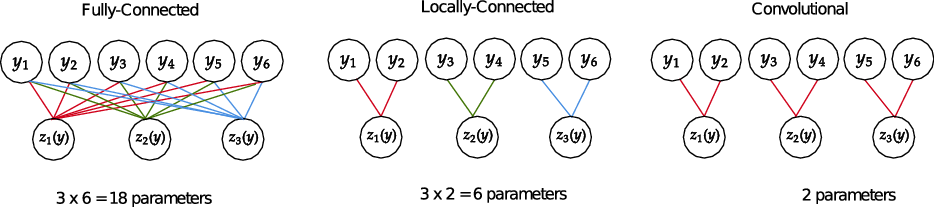
Figure 1 graphically shows how the three different layers work. For illustrative purposes, we consider a 6-dimensional input vector (which can be seen as an array of size
 $1 \times 6 \times 1$
when we apply LCN and CNN layers). For the FCN, we set the layer’s size equal to 3, while for the LCN and CNN network, we set the kernel size and stride equal
 $m= s= 2$
and the number of filters
 $q = 1$
. In the FCN layer, each unit is connected to all input units, and the total number of parameters to learn in the layer (excluding bias terms) is 18. The LCN layer introduces local connectivity, and each unit is connected to only two units of the input layer without overlapping. In this case, the number of parameters is 6. CNN imposes also parameter sharing, and the weights are the same for all the units. In this case, the layer has only 2 parameters. A more detailed description of these layers can be found in Goodfellow et al. (Reference Goodfellow, Bengio and Courville2016).
Layer architecture and number of parameters for the fully connected (left), locally connected (middle) and convolutional (right) NNs. The total number of parameters does not include the bias terms for all three layers.

3.4. Embedding network
Data often present categorical variables. Examples in mortality modelling context are the region
 $r \in \mathcal{R}$
and the gender
 $g \in \mathcal{G}$
to which a particular mortality rate refers. Dummy coding or one-hot encoding are popular approaches to deal with categorical variables among statisticians and the machine learning community, respectively. However, when observations present many categorical variables or when the variables have many different labels, these coding schemes produce high-dimensional sparse vectors, which often causes computational and calibration difficulties.
Embedding layers provide an elegant way to deal with categorical input variables. They are already intensively employed in Natural Language Processing (Bengio et al., Reference Bengio, Ducharme, Vincent and Jauvin2003) and recently are introduced in the actuarial literature by Richman, see Richman (Reference Richman2020a); Richman (Reference Richman2020b). In essence, they allow learning a low-dimensional representation of a categorical variable. Thereby, every level of the considered categorical variable is mapped to a vector in
 $\mathbb{R}^{q_\mathcal{P}}$
for some
 $q_\mathcal{P} \in \mathbb{N}$
. These vectors are then simply parameters of the NN that have to be trained (Guo and Berkhahn, Reference Guo and Berkhahn2016). In the new space learned by the embedding layer, labels similar for the task of interest present a small Euclidean distance while different labels present a larger one.
Formally, let
 $\mathcal{P} = \{p_1, p_2,\dots, p_{n_\mathcal{P}} \}$
be the (finite) set of categories of the qualitative variable and
 $n_\mathcal{P} = |\mathcal{P}|$
be its the cardinality. An embedding layer is a mapping
 \begin{align*}\boldsymbol{z}_\mathcal{P} \;:\; \mathcal{P} \to \mathbb{R}^{q_\mathcal{P} }, \quad \quad p \mapsto \boldsymbol{z}_\mathcal{P}(p),\end{align*}
where
 $q_\mathcal{P} \in \mathbb{N}$
is a hyper-parameter denoting the size of the embedding layer. The number of embedding weights that must be learned during training is
 $n_\mathcal{P} q_\mathcal{P}$
and the embedding size is typically
 $q_\mathcal{P} \ll n_\mathcal{P}$
.
4. The neural network approach for ILC models fitting
In this section, we introduce the proposed general NN architecture for the ILC models fitting. In this regard, we keep the same notation introduced in Section 2 and consider different populations indexed by
 $i \in \mathcal{I}$
, where populations may differ in gender
 $g \in \mathcal{G}= \{\texttt{male}, \texttt{female}\}$
and country
 $r \in \mathcal{R}$
such that
 $i = (r,g) \in \mathcal{I} = \mathcal{R} \times \mathcal{G}$
.
4.1. Model formalisation
We develop a N that models the mortality of many populations by replicating the ILC models’ structure. The mortality of each population is modelled by an own LC model; however, unlike the standard approach, the model fitting is performed in a single stage using all available mortality data. Each mortality experience processed by the network consists of the curve of the log-mortality rates for all ages
 $\log\left(\boldsymbol{m}_t^{(i)}\right) = \left( \log\!\left(m_{x,t}^{(i)}\right) \right)_{x \in \mathcal{X}}$
and the gender and region labels, respectively,
 $r \in \mathcal{R}$
and
 $g\in \mathcal{G}$
, that identify uniquely the population
 $i = (r, g) \in \mathcal{I}$
.
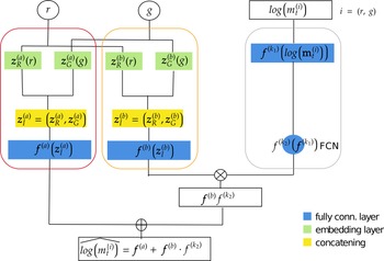
The network architecture, based on the blocks described in Section 3, can be conceptually divided into three subnets which process the data inputs separately. Each one of these subnets aims to extract one component of the model in (2.5). More in details, the outputs of first two subnets substitute
 $\boldsymbol{a}^{(i)} = \left(a_x^{(i)}\right)_{x \in \mathcal{X}} \in \mathbb{R}^{|\mathcal{X}|}$
and
 $\boldsymbol{b}^{(i)} = \left(b_x^{(i)}\right)_{x \in \mathcal{X}} \in \mathbb{R}^{|\mathcal{X}|}$
. Since these LC parameters depend only on the population i, these subnets process only the region and gender labels. The outputs of these two subnets are two time-independent vectors that present as many components as the ages considered. The third subnet aims to extract the factor
 $k_t^{(i)} \in \mathbb{R}$
, which summaries the mortality dynamics at time t in the population i. In this case, the subnet takes as input the curve of log-mortality rates
 $\log\!(\textbf{m}_t^{(i)})\in \mathbb{R}^{|\mathcal{X}|}$
in the population i at time t and produces as output a single value. In other words, this subnet encodes the curve of the log-mortality rates into a real value. Finally, the extracted factors are combined to provide an approximation of the log-mortality rates’ curve using the functional form of the LC model.
A pictorial representation of the network architecture is illustrated in Figure 2, while a formal description is provided below.
Graphical representation of the neural network architecture for ILC models fitting.

In details, the first subnet, (confined within the red diagram) is called
 $\textbf{a}^{(i)}$
-subnet and consists of two embedding layers and a FCN layer. Formally, let
 $q^{(a)}_{\mathcal{R}}, q^{(a)}_{\mathcal{G}} \in \mathbb{N}$
be the hyper-parameter values defining the size of the two embedding layers, they map
 $r \in \mathcal{R}$
and
 $g \in \mathcal{G}$
into real-valued vectors:
 \begin{eqnarray*} \boldsymbol{z}_{\mathcal{R}}^{(a)}\;:\;\mathcal{R} \to \mathbb{R}^{q^{(a)}_{\mathcal{R}}}, &&\quad \quad r \mapsto \boldsymbol{z}^{(a)}_{\mathcal{R}}(r) =\left( z^{(a)}_{{\mathcal{R}},1}(r), z^{(a)}_{{\mathcal{R}},2} (r), \dots , z^{(a)}_{{\mathcal{R}},q^{(a)}_{\mathcal{R}}}(r) \right)^\top,\\ \boldsymbol{z}_{\mathcal{G}}^{(a)}\;:\;\mathcal{G} \to \mathbb{R}^{q^{(a)}_{\mathcal{G}}}, &&\quad \quad g \mapsto \boldsymbol{z}^{(a)}_{\mathcal{G}}(g) =\left( z^{(a)}_{{\mathcal{G}},1}(g), z^{(a)}_{{\mathcal{G}},2} (g), \dots , z^{(a)}_{{\mathcal{G}},q^{(a)}_{\mathcal{G}}}(g) \right)^\top.\end{eqnarray*}
Since
 $\boldsymbol{z}_{\mathcal{R}}^{(a)}(r)$
is a new set of features representing the region r and
 $\boldsymbol{z}_{\mathcal{G}}^{(a)}(g)$
is a new representation of the gender g, the vector
 $\boldsymbol{z}_{\mathcal{I}}^{(a)} = \boldsymbol{z}_{\mathcal{I}}^{(a)} (r, g) = \Big(\!\left(\boldsymbol{z}_{\mathcal{R}}^{(a)}(r)\right)^\top, $
 $\left(\boldsymbol{z}_{\mathcal{G}}^{(a)}(g)\right)^\top\Big)^\top\in \mathbb{R}^{q^{(a)}_{\mathcal{I}}} $
(with
 $q_{\mathcal{I}}^{(a)} = q_{\mathcal{R}}^{(a)} +q_{\mathcal{G}}^{(a)}$
), obtained concatenating the output of these two embedding layers, can be understood as a learned representation of the population
 $i = (r, g)$
. It is then processed by a FCN layer which provides as many units as the age considered. This layer maps
 $\boldsymbol{z}_{\mathcal{I}}^{(a)}$
in a new
 $|\mathcal{X}|$
-dimensional real-valued space
 \begin{align*} & \boldsymbol{f}^{(a)}\;:\;\mathbb{R}^{q^{(a)}_{\mathcal{I}}} \to \mathbb{R}^{|\mathcal{X}|},\\ & \boldsymbol{z}^{(a)}_{\mathcal{I}} \mapsto \boldsymbol{f}^{(a)}\left(\boldsymbol{z}^{(a)}_{\mathcal{I}}\right) = \left(f^{(a)}_{x_{0}}\left(\boldsymbol{z}^{(a)}_{\mathcal{I}}\right), f^{(a)}_{x_{1}} \left(\boldsymbol{z}^{(a)}_{\mathcal{I}}\right), \dots , f^{(a)}_{x_{\omega}}\left(\boldsymbol{z}^{(a)}_{\mathcal{I}}\right) \right)^\top.\end{align*}
Each new feature
 $f^{(a)}_x\left(\boldsymbol{z}^{(a)}_{\mathcal{I}}\right)$
is a age-specific function of the vector
 $\boldsymbol{z}^{(a)}_{\mathcal{I}}$
 \begin{align}\boldsymbol{z}^{(a)}_{\mathcal{I}}\;\mapsto\;f^{(a)}_x(\boldsymbol{z}^{(a)}_{\mathcal{I}}) & =\phi^{(a)} \left( w^{(a)}_{x,0} + \sum_{l = 1}^{q_{\mathcal{I}}^{(a)}} w^{(a)}_{x,l} z^{(a)}_{\mathcal{I}, l} \right)\nonumber \\ & = \phi^{(a)} \left( w^{(a)}_{x,0} + \left\langle \boldsymbol{w}^{(a)}_x, \boldsymbol{z}^{(a)}_{\mathcal{I}} \right\rangle \right), \quad x \in \mathcal{X},\end{align}
where
 $\phi^{(a)}\;:\;\mathbb{R} \to \mathbb{R}$
is a (non-linear) activation function,
 $w^{(a)}_{x,l} \in \mathbb{R}$
are the network parameters.
The output of this layer is a vector that contains as many components as the ages considered. Although all the units in the FCN layer process the population-specific features
 $\boldsymbol{z}^{(a)}_{\mathcal{I}}$
, the coefficients
 $w^{(a)}_{x,0}$
and
 $\boldsymbol{w}^{(a)}_x$
differ from neuron to neuron and are age-specific. This means that the output of each neuron
 $f^{(a)}_x\left(\boldsymbol{z}^{(a)}_{\mathcal{I}}\right)$
is, in fact, an age and population-specific function as the
 $a_x^{(i)}$
parameter of the LC model. The output of the whole layer
 $ \boldsymbol{f}^{(a)}\left(\boldsymbol{z}^{(a)}_{\mathcal{I}}\right) = \left( f^{(a)}_{x}\left(\boldsymbol{z}^{(a)}_{\mathcal{I}}\right)\right)_{x \in \mathcal{X}}$
, obtained by concatenating the output of all the age-specific units, is similar to the vector
 $\textbf{a}^{(i)} = \left(a_x^{(i)}\right)_{x\in \mathcal{X}}$
and can be considered as a population-specific term only.
The second subnet (confined within the orange diagram) is called
 $\textbf{b}^{(i)}$
-subnet and presents the same architecture of the first one. We will use the upper index (b) to denote the quantities referring to this subnet for distinguishing them from the previous one. It provides two embedding layers of size
 $q^{(b)}_{\mathcal{R}}, q^{(b)}_{\mathcal{G}} \in \mathbb{N}$
and a
 $|\mathcal{X}|$
-dimensional FCN layer which takes the vector
 $\boldsymbol{z}_{\mathcal{I}}^{(b)} = \boldsymbol{z}_{\mathcal{I}}^{(b)} (r, g) = \Big(\Big(\boldsymbol{z}_{\mathcal{R}}^{(b)}(r)\big)^\top,\Big(\boldsymbol{z}_{\mathcal{G}}^{(b)}(g)\Big)^\top \Big)^\top\in \mathbb{R}^{q^{(b)}_{\mathcal{I}}} $
 $\Big(\textrm{with}\;q_{\mathcal{I}}^{(b)} = q_{\mathcal{R}}^{(b)} +q_{\mathcal{G}}^{(b)}\Big)$
. It is important to remark that, despite the first two subnets present the same architecture, the weights to learn in each layer are different.
Denoting by
 $\boldsymbol{w}^{(j)}_{0} = (w^{(j)}_{x,0} )_{x \in \mathcal{X}} \in \mathbb{R}^{\mid \mathcal{X} \mid }$
and
 $W^{(j)} = (w^{(j)}_{x,l} )_{x \in \mathcal{X}, l = 1, \dots, q_{\mathcal{I}}^{(j)}} \in \mathbb{R}^{ \mid \mathcal{X} \mid \times q^{(j)}_{\mathcal{I}}}$
,
 $\forall j \in \{a,b\}$
, the output of the first two subnets can be written in compact form
 \begin{align} \boldsymbol{f}^{(a)} \big( \boldsymbol{z}_{\mathcal{I}}^{(a)} \big) &= \phi^{(a)} \bigg( \boldsymbol{w}^{(a)}_{0} + \left\langle W^{(a)}, \boldsymbol{z}_{\mathcal{I}}^{(a)} \right\rangle \bigg) \nonumber \\ &= \phi^{(a)} \bigg( \boldsymbol{w}_{0}^{(a)}+\left\langle W_{\mathcal{R}}^{(a)} , \boldsymbol{z}_{\mathcal{R}}^{(a)} (r) \right\rangle + \left\langle W_{\mathcal{G}}^{(a)} , \boldsymbol{z}_{\mathcal{G}}^{(a)} (g) \right\rangle \bigg),\end{align}
 \begin{align} \boldsymbol{f}^{(b)} \big( \boldsymbol{z}_{\mathcal{I}}^{(b)} \big) & = \phi^{(b)} \bigg( \boldsymbol{w}^{(b)}_{0} + \left\langle W^{(b)}, \boldsymbol{z}_{\mathcal{I}}^{(b)} \right\rangle \bigg) \nonumber \\ & = \phi^{(b)} \bigg( \boldsymbol{w}_{0}^{(b)}+\left\langle W_{\mathcal{R}}^{(b)} , \boldsymbol{z}_{\mathcal{R}}^{(b)} (r) \right\rangle + \left\langle W_{\mathcal{G}}^{(b)} , \boldsymbol{z}_{\mathcal{G}}^{(b)} (g) \right\rangle \bigg),\end{align}
where one could carry out the decomposition
 $W^{(j)} = \big( W_{\mathcal{R}}^{(j)}, W_{\mathcal{G}}^{(j)} \big)$
of the matrices of the FCN layers to distinguish the weights which refer to the gender-specific and the region-specific features.
The architecture of the third subnet (inside the grey diagram) is different from the previous ones. We call it
 $k_t^{(i)}$
-subnet. It consists of some stacked feed-forward NN layers that process the log-mortality rates curve. In this case, a large discretionary in the number and type of NN layers to employ is left to the modeller. For the sake of simplicity, we described the model considering two FCN layers and postponed a comparative discussion with the LCN and CNN layers to the numerical experiments’ section. Let
 $q_{z_1}\in \mathbb{N}$
and
 $ q_{z_2} = 1$
be two hyper-parameters defining the size of two FCN layers. The first FCN layer maps
 $\log\!(\boldsymbol{m}_{t}^{(i)})$
into a
 $q_{z_1}$
-dimensional real-valued space:
 \begin{align*} &\boldsymbol{f}^{(k_1)} \;:\; \mathbb{R}^{|\mathcal{X}|} \to \mathbb{R}^{q_{z_1}}, \\ & \log\!\left(\boldsymbol{m}_{t}^{(i)}\right)\; \mapsto\; \boldsymbol{f}^{(k_1)} \left(\log\!\left(\boldsymbol{m}_{t}^{(i)}\right)\right) = \left(f^{(k_1)}_1\left(\log\!\left(\boldsymbol{m}_{t}^{(i)}\right)\right), \dots , f^{(k_1)}_{q_{z_1}}\left(\log\!\left(\boldsymbol{m}_{t}^{(i)}\right) \right) \right)^\top,\end{align*}
where each new feature component
 $f^{(k_1)}_s(\log\!(\boldsymbol{m}_{t}^{(i)}))$
is function of the mortality rates of all ages
 \begin{align} \log\!\left(\boldsymbol{m}_{t}^{(i)}\right)\;\mapsto\; f^{(k_1)}_s\left(\!\log\!(\boldsymbol{m}_{t}^{(i)})\right) &= \phi^{(k_1)} \left(w^{(k_1)}_{s,0} + \left\langle \boldsymbol{w}^{(k_1)}_s, \log\!(\boldsymbol{m}_{t}^{(i)}) \right\rangle \right), \nonumber\\ s & = 1, \dots , q_{z_1},\end{align}
where
 $w^{(k_1)}_{s,0} \in {\mathbb R}$
and
 $\boldsymbol{w}^{(k_1)}_s \in \mathbb{R}^{|\mathcal{X}|}$
are parameters. Otherwise, by using LCN layer we would obtain new features which are functions of a segment of the log-mortality curve. The second FCN layer of size
 $q_{z_2} = 1$
is a mapping
 \begin{align*} & f^{(k_2)} \;:\; \mathbb{R}^{q_{z_1}} \to \mathbb{R},\\ & \boldsymbol{f}^{(k_1)} \left(\!\log\!(\boldsymbol{m}_{t}^{(i)}) \right) \mapsto f^{(k_2)} \left(\,\boldsymbol{f}^{(k_1)} \left(\!\log\!(\boldsymbol{m}_{t}^{(i)}) \right)\right) = \left(\,f^{(k_2)} \circ \boldsymbol{f}^{(k_1)}\right) \left(\log\!(\boldsymbol{m}_{t}^{(i)})\right).\end{align*}
It extracts a single new feature
 \begin{equation} (f^{(k_2)} \circ \boldsymbol{f}^{(k_1)}) \left(log\!\left(\boldsymbol{m}_{t}^{(i)}\right)\!\right) = \phi^{(k_2)} \left(\!w^{(k_2)}_0 + \left\langle \boldsymbol{w}^{(k_2)}, \phi^{(k_1)} \left(\!\boldsymbol{w}^{(k_1)}_0 + W^{(k_1)} \log\!\left(\!\boldsymbol{m}_{t}^{(i)}\right)\!\right) \right\rangle\right)\!,\end{equation}
where
 $w_0^{(k_2)} \in \mathbb{R},\!\boldsymbol{w}_0^{(k_1)} = (w_{s,0}^{(k_1)})_{1\leq s \leq q_{z_1}}\in \mathbb{R}^{q_{z_1}},\!\boldsymbol{w}^{(k_2)}\in \mathbb{R}^{q_{z_1}},\!W^{(k_1)} = (\boldsymbol{w}_s^{(k_1)})^{\top}_{1\leq s \leq {q_{z_1}}}$
 $ \in \mathbb{R}^{q_{z_1} \times \mid \mathcal{X} \mid}$
are network parameters and
 $\phi^{(j)}(\!\cdot\!)\;:\;\mathbb{R} \to \mathbb{R}$
for
 $j \in \{k_1, k_2\}$
are activation functions. Basically, the first FCN layer encodes the log-mortality curve into a
 $q_{z_1}$
-dimensional real-valued vector, the second layer further compresses this results into in a single real value.
Finally, an approximation of log-mortality curve at time t in the population i can be obtained as
 \begin{equation}\begin{split} \widehat{ \log\!\left(\boldsymbol{m}_{t}^{(i)}\right)}= \boldsymbol{f}^{(a)} \left(\boldsymbol{z}_{\mathcal{I}}^{(a)}\right) + \boldsymbol{f}^{(b)} \left(\boldsymbol{z}_{\mathcal{I}}^{(b)} \right) (f^{(k_2)} \circ \boldsymbol{f}^{(k_1)}) \left(\!\log\!\left(\boldsymbol{m}_{t}^{(i)}\right)\right),\end{split}\end{equation}
where each age component is given by
 \begin{equation}\begin{split} \widehat{ \log\!({m}_{x,t}^{(i)})}= f_x^{(a)} \left(\boldsymbol{z}_{\mathcal{I}}^{(a)}\right) + f_x^{(b)} \left(\boldsymbol{z}_{\mathcal{I}}^{(b)}\right) \left(f^{(k_2)} \circ \boldsymbol{f}^{(k_1)}\right) \left(\!\log\!\left(\boldsymbol{m}_{t}^{(i)}\right)\right).\end{split}\end{equation}
A simple interpretation of all terms in (4.7) can be provided:
-
 $ f_x^{(a)}\left(\boldsymbol{z}_{\mathcal{I}}^{(a)}\right)\in \mathbb{R}$
is a population and age-specific term that plays the same role of
${a}_x^{(i)}$
in the LC model.
-
$ f_x^{(b)} \left(\boldsymbol{z}_{\mathcal{I}}^{(b)}\right) \in \mathbb{R}$
is a population and age-specific term that plays the same role of
$b_x^{(i)}$
in the LC model.
-
$ \left(f^{(k_2)} \circ \boldsymbol{f}^{(k_1)}\right) \left(\log\!\left(\boldsymbol{m}_{t}^{(i)}\right)\right) \in \mathbb{R}$
is a population and time-specific term that plays the same role of the
$k_t^{(i)}$
in the LC model.


Similarly, Equation (4.6) is the LC model written in compact form where the output of the first subnet
 $\boldsymbol{f}^{(a)}\left(\boldsymbol{z}_{\mathcal{I}}^{(a)}\right) \in \mathbb{R}^{|\mathcal{X}|}$
plays the same role of the vector of parameters
 $\boldsymbol{a}^{(i)}= \left(a_x^{(i)}\right)_{x \in \mathcal{X}} $
and the output of the second subnet
 $\boldsymbol{f}^{(b)}\big(\boldsymbol{z}_{\mathcal{I}}^{(b)} \big) \in \mathbb{R}^{|\mathcal{X}|}$
plays the same role of the vector
 $\boldsymbol{b}^{(i)}= \big( b_x^{(i)} \big)_{x \in \mathcal{X}} $
.
In addition, setting linear activation
 $\phi^{(j)}(x)=x, \ \forall j \in \{a,b\}$
and expanding all the terms in (4.7), the model can be written as
 \begin{equation*} \widehat{ \log\!({m}_{x, t}^{(i)})}= \bigg( w^{(a)}_{x,0} + \left\langle \boldsymbol{w}_x^{(a)}, \boldsymbol{z}_{\mathcal{I}}^{(a)} \right\rangle \bigg)\ + \end{equation*}
 \begin{equation}+ \bigg( w^{(b)}_{x,0} + \left\langle \boldsymbol{w}_x^{(b)}, \boldsymbol{z}_{\mathcal{I}}^{(b)} \right\rangle \bigg) \cdot \phi^{(k_2)} \bigg( w^{(k_2)}_0 + \left\langle \boldsymbol{w}^{(k_2)}, \phi^{(k_1)} \bigg( \boldsymbol{w}^{(k_1)}_0 + W^{(k_1)} \log\!(\boldsymbol{m}_{t}^{(i)}) \bigg) \right\rangle \bigg).\end{equation}
In this case, some further interpretations can be argued. The term
 $\bigg( w^{(a)}_{x,0} + \left\langle \boldsymbol{w}_x^{(a)}, \boldsymbol{z}_{\mathcal{I}}^{(a)} \right\rangle \bigg)$
can be further decomposed into
 ${w}^{(a)}_{x, 0}$
, which can be interpreted as a population-independent
 $a_x$
parameter, and
 $ \left\langle \boldsymbol{w}_x^{(a)}, \boldsymbol{z}_{\mathcal{I}}^{(a)}\right\rangle =\left\langle \boldsymbol{w}_{x,\mathcal{R}}^{(a)}, \boldsymbol{z}_{\mathcal{R}}^{(a)}(r)\right\rangle+\left\langle\boldsymbol{w}_{x,\mathcal{G}}^{(a)}, \boldsymbol{z}_{\mathcal{G}}^{(a)}(g) \right\rangle$
, which can be interpreted as a population-specific
 $a_x$
correction. In particular, it is the sum of the region-specific correction term
 $\left\langle\boldsymbol{w}_{x,\mathcal{R}}^{(a)}, \boldsymbol{z}_{\mathcal{R}}^{(a)} (r)\right\rangle$
and the gender-specific correction term
 $\left\langle\boldsymbol{w}_{x,\mathcal{G}}^{(a)}, \boldsymbol{z}_{\mathcal{G}}^{(a)} (r)\right\rangle$
. The same decomposition can be applied to
 $\bigg( w^{(b)}_{x,0} + \left\langle \boldsymbol{w}_x^{(b)}, \boldsymbol{z}_{\mathcal{I}}^{(b)} \right\rangle \bigg)$
.
4.2. Model fitting and forecasting
As anticipated in the previous sections, the NN model’s performance depends on the network parameters that must be appropriately calibrated. Denoting by
 $\psi$
the full set of the network model’s parameters described above, it can be split into two groups. The first group concerns the population-specific parameters, namely the embedding parameters,
 $\boldsymbol{z}^{(a)}_{\mathcal{R}}(r), \boldsymbol{z}^{(b)}_{\mathcal{R}}(r)$
and
 $\boldsymbol{z}^{(a)}_{\mathcal{G}}(g), \boldsymbol{z}^{(b)}_{\mathcal{G}}(g)$
which contribute only to the population-specific LC model. The remaining
 $\boldsymbol{w}^{(j)}_{0}, W^{(j)},\boldsymbol{w}^{(k_2)}$
and
 $ w^{(k_2)}_0$
are cross-population parameters which contribute to all the individual LC models. These parameters are iteratively adjusted via the BP algorithm to minimise a given loss function. During the training, we also apply the dropout (Srivastava et al., Reference Srivastava, Hinton, Krizhevsky, Sutskever and Salakhutdinov2014) in some layers of the networks to regularise. The dropout is a powerful regularisation technique which has produced notable results in several applications such as image processing and speech recognition (Pham et al., Reference Pham, Bluche, Kermorvant and Louradour2014). It consists of ignoring some randomly chosen units during the network fitting. The use of the dropout during the NN training allows to extract more robust features from the data and avoid overfitting (Srivastava et al., Reference Srivastava, Hinton, Krizhevsky, Sutskever and Salakhutdinov2014). In our application, it contributes to obtain more robust estimates of LC parameters which appear smoother over the age dimension and less sensitive to the fluctuations often present in the mortality data compared to traditional fitting schemes.
This technique forces a NN to learn more robust features and prevent overfitting. Once the model training was completed, and an estimation of the optimal set of parameters
 $\hat{\psi}$
was obtained, population-specific parameters and cross-population parameters can be used to compute the terms in the model presented in (4.7). Since these quantities have the same meaning as the LC model terms, we could consider them as NN estimates of the LC parameters:
 \begin{equation} \hat{a}_{x, NN}^{(i)} = \phi^{(a)} \bigg( \hat{w}_{x, 0}^{(a)}+\left\langle \hat{\boldsymbol{w}}_{x,\mathcal{R}}^{(a)}, \hat{\boldsymbol{z}}_{\mathcal{R}}^{(a)} (r) \right\rangle + \left\langle \hat{\boldsymbol{w}}_{x,\mathcal{G}}^{(a)}, \hat{\boldsymbol{z}}_{\mathcal{G}}^{(a)} (g) \right\rangle \bigg), \quad \forall x \in \mathcal{X}, \forall i \in \mathcal{I},\end{equation}
 \begin{equation}\kern-10pt\hat{b}_{x, NN}^{(i)} = \phi^{(b)} \bigg( \hat{w}_{x, 0}^{(b)}+\left\langle \hat{\boldsymbol{w}}_{x,\mathcal{R}}^{(b)}, \hat{\boldsymbol{z}}_{\mathcal{R}}^{(b)} (r) \right\rangle + \left\langle \hat{\boldsymbol{w}}_{x,\mathcal{G}}^{(b)}, \hat{\boldsymbol{z}}_{\mathcal{G}}^{(b)} (g) \right\rangle \bigg), \quad \forall x \in \mathcal{X}, \forall i \in \mathcal{I},\end{equation}
 \begin{equation} \hat{k}_{t, NN}^{(i)} = \phi^{(k_2)} \bigg( \hat{w}^{(k_2)}_0 + \left\langle \hat{\boldsymbol{w}}^{(k_2)}, \phi^{(k_1)} \bigg( \hat{\boldsymbol{w}}^{(k_1)}_0 + \hat{W}^{(k_1)} \log\!(\boldsymbol{m}_{t}^{(i)}) \bigg) \right\rangle \bigg),\!\! \quad \forall t \in \mathcal{T}, \forall i \in \mathcal{I}.\end{equation}
The classical LC constraints (Lee and Carter, Reference Lee and Carter1992) are applied to the NN estimates of the LC parameters individually for each population. We do not modify the time-series part of the ILC approach; forecasting is performed assuming that
 $\hat{a}_{x, NN}^{(i)}$
and
 $\hat{b}_{x, NN}^{(i)}$
are constant over time while
 $\hat{k}_{t, NN}^{(i)}$
is projected with a random walk with drift for each population. It is interesting to note that often the number of LC parameters
 $\left(a_x^{(i)}\right)_x, \left(b_x^{(i)}\right)_x, \left(k_t^{(i)}\right)_t$
, for each population, can be larger than the number of network weights.
5. Numerical experiments
In this section, some numerical experiments to validate the proposed approach are conducted.
The data source is the HMD, which provides mortality data for male and female populations of a large set of countries. Following the experiments’ scheme in Perla et al. (Reference Perla, Richman, Scognamiglio and Wüthrich2021), Richman and Wüthrich (Reference Richman and Wüthrich2021), we only consider mortality data from 1950 onwards, and we set 1999 as the final observation year.
Let
 $\mathcal{T} = \{ t \in {\mathbb N}\;:\; 1950 \leq t \leq 2019\}$
be the full set of available years and
 $\mathcal{T}_{1} = \left\{ t \in \mathcal{T}\;:\; t <2000\right\}, \mathcal{T}_{2} = \{ t \in \mathcal{T}\;:\; t \geq 2000\}$
such that
 $\mathcal{T}_{1} \cup \mathcal{T}_{2} = \mathcal{T}$
. The aim is to forecast, as accurately as possible, the mortality rates of calendar years in
 $\mathcal{T}_{2}$
using a model fitted on mortality data of calendar years in
 $\mathcal{T}_{1}$
. Using the machine learning terminology, the mortality rates of calendar years in
 $\mathcal{T}_{1}$
represent the training set, while the mortality rates of calendar years in
 $\mathcal{T}_{2}$
represent the testing set.
First, a careful round of data pre-processing was carried out. We consider only male and female populations of countries for which at least 10 calendar years of mortality data before 1999 are available. We define
 $\mathcal{R} $
as the set of selected countries and, in our experiments, we observe that
 $|\mathcal{R}|= 40$
and
 $|\mathcal{I}| = 80$
since
 $\mathcal{I} = \mathcal{R} \times \mathcal{G} = \mathcal{R} \times \{ \texttt{male}, \texttt{female}\}$
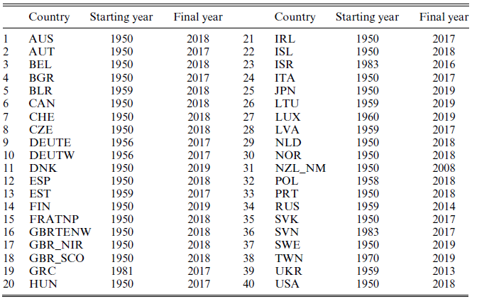
. The full list of countries in
 $\mathcal{R}$
can be found in Table A.1 in Appendix A. Furthermore, only ages in
 $\mathcal{X} = \left\{ x \in \mathbb{Z} \;:\; 0 \leq x < 100 \right\}$
were considered (with
 $|\mathcal{X}| = 100$
) and, following the scheme adopted in Perla et al. (Reference Perla, Richman, Scognamiglio and Wüthrich2021), Richman and Wüthrich (Reference Richman and Wüthrich2021), mortality rates recorded as zero or missing were imputed using the average rate at that age across all countries for that gender in that year.
After the pre-processing stage, we discuss the NN models that we experimented with. Since no golden rules exist for NN design, several architectures were investigated and compared. The first difference among them concerns the architecture of the third subnet, which processes the log-mortality curve
 $\log\!\left(\boldsymbol{m}_{t}^{(i)}\right) $
:
-
The first group of networks, called LC_FCN networks, use two FCN layers as the architecture described in Section 4.
-
The second class of networks replaces the first FCN layer in the third subnet with an LCN layer. In this case, the curve
$\log\!\left(\boldsymbol{m}_{x}^{(i)}\right) $
is processed by an LCN layer where the local connectivity is applied to the age-related dimension. It appears reasonable to believe that a successful features extraction can be obtained by processing separately small segments of the log-mortality curve. We set the number of filters
$q=1$
and the kernel size equal to the stride
$m = s= G$
. In this setting, there is no overlap between adjacent receptive fields, and the layer extracts a feature from each group of G adjacent ages (e.g., if we have
$G = 4$
the age groups are
$0-3, 4-7, \dots, 96-99$
). The size of the output of this layer
$q_{z_1}$
can be controlled through G since
$q_{z_1} = |\mathcal{X}|/G$
. An FCN further processes the output of this layer as in the LC_FCN model. The adoption of the LCN layer involves a significant reduction of the parameters to optimise due to the local connectivity. We call this variant LC_LCN. -
The latest group of architectures substitutes the first LCN layer of the third subnet with a CNN layer keeping the same hyper-parameter setting of the LCN layer-based model. In this case, the features extracted from the different G-sized age groups are obtained using the same set of parameters. This further reduces the number of parameters to learn with respect to the LCN layer since the CNNs are characterised by local connectivity and weight sharing. This variant is named LC_CNN.


We also explore the role of other hyper-parameters:
-
the size of the embedding layers
$q_e \in \{5,10\}$
, where
$q_e = q^{(a)}_{\mathcal{R}} = q^{(a)}_{\mathcal{G}} = q^{(b)}_{\mathcal{R}} = q^{(b)}_{\mathcal{G}}$
; -
the dimension of the first layer of the third subnet
$q_{z_1} \in \{10,25,50\}$
Footnote 1; -
the activation function of the first layer of the third subnet
$\phi^{(k_1)} \in \left\{'linear', 'ReLU', 'tanh' \right\}$
.


Overall, 54 different architectures are considered. We consider linear activation for the FCN layer in the first two subnet and the second layer of the
 $k_t^{(i)}$
-subnet,
 $\phi^{(j)}(x) = x \ \forall j \in \{a, b, k_2 \}$
. All the analyses are carried out in the R environment, and the NN models considered were developed using the R package keras (Chollet, Reference Chollet2018).
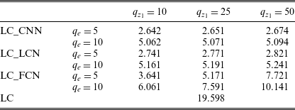
Table 1 reports the total number of network weights for each NN model defined above. First, we observe that the differences between the number of parameters of the LC_FCN and LC_LCN networks are pretty significant. This means that by introducing local connectivity in the first layer of the third subnet, a large part of the parameters can be saved. On the contrary, the differences between LC_LCN and LC_CNN networks are generally small. Then, the further reduction of the number of weights induced by the weight sharing mechanism is quite limited. In addition, it can be noted that the number of parameters increases for all the three network categories when
 $q_e$
and
 $q_{{z_1}}$
increase.
Number of network parameters for the neural network models considered.

5.1. MSE minimisation
All the network models are fitted in the first stage, minimising the Mean Squared Error (MSE). The training sample includes 3598 mortality examples which are processed for 2000 epochs. We do not use any strategy to fight the overfitting since all the network models considered present very few parameters to optimise, and the risk of overfitting is absent. The choice of the MSE as loss function can be motivated by arguing that the original paper suggests fitting the LC model using the SVD to perform the PCA. Since the PCA can be expressed as an optimisation problem, in which the MSE between the original data and the data reconstructed using an approximating linear, the use of the MSE as loss function appears reasonable. Furthermore, it is remarkable that the MSE minimisation is equivalent to the likelihood maximising in the Gaussian assumption of the mortality rates (Richman and Wüthrich, Reference Richman and Wüthrich2021).
In this setting, the network training involves the minimisation of the following loss function
 \begin{equation*}{L(\psi) = \sum_{x \in \mathcal{X}} \sum_{i \in \mathcal{I}} \sum_{t \in \mathcal{T}} \bigg( \log\!({m}_{x,t}^{(i)}) - \widehat{ \log\!({m}_{x, t}^{(i)})} \bigg)}{^2},\end{equation*}
where
 $ \widehat{ \log\!({m}_{x, t}^{(i)})}$
is defined by (4.8). The Adam optimiser algorithm (Kingma and Ba, Reference Kingma and Ba2014) with the parameter values taken at the defaults is used. When we use the MSE loss function to train the networks, we add the label “_mse” to of all the NN models’ names.
Once the network fitting is completed, and the set of the optimal network parameters is estimated, the corresponding NN estimations of the LC parameters can be computed accordingly with Equations (4.9), (4.10) and (4.11).Footnote 2 Forecasting is performed as described in Section 4, and the performance of the different models is measured by the MSE between the predicted mortality rates and the actual ones.
In this setting, we define the response variable scaled in [0, 1] as in Perla et al. (Reference Perla, Richman, Scognamiglio and Wüthrich2021). This does not modify the general model but induces some changes in the formulas for the NN estimates of LC parameters. Details can be found in Appendix B.
5.1.1. Results
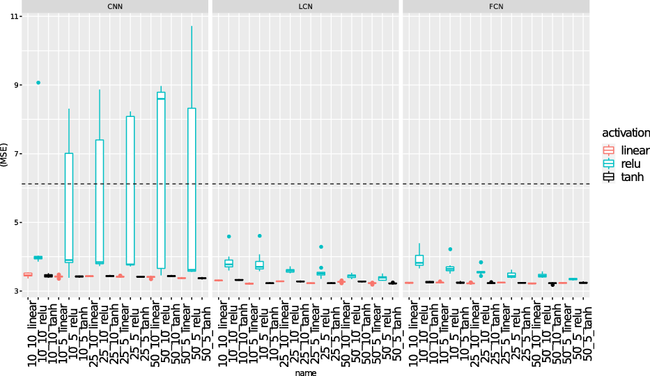
In this section, we discuss the results of the numerical experiments. Since the out-of-sample results of the NN models can vary among training attempts due to the randomness of some elements of the training process (i.e., the random selection of batches of training data, dropout, the initial value of optimisation algorithm and others), we first analyse and measure the variability of these results. For this purpose, 10 different model fittings for each one of the 54 network models considered are performed and the boxplots of the corresponding forecasting MSEs are visualised in Figure 3. In particular, this figure provides three groups of subplots, one of each group of networks investigated and a dashed line indicating the forecasting performance of the standard LC methodology via SVD henceforth indicated as LC_SVD. Some interesting comments can be made. First, we observe that most boxplots lie below the dotted line suggesting that the corresponding network models produce forecasting MSEs significantly lower than the LC_SVD model. In addition, the variability among training attempts appears to be quite limited in most cases. Second, comparing the networks models among them, we note that the LC_LCN_mse and LC_FCN_mse models, which produce very similar results, overperform the LC_CNN_mse models. This result probably suggests that some of the network parameters employed by the LC_FCN_mse models are redundant and the reduction in the number of parameters induced by the local connectivity does not deteriorate the performance. On the contrary, the further reduction induced by the weight sharing mechanism, on which the LC_CNN_mse models are based, produces a slight deterioration in performance. We believe this may be because using the same set of parameters for all the age groups we could reduce the quality of the feature extraction. This argument appears plausible since the mortality rates in different ages present different features. Third, analysing the robustness with respect to the hyper-parameters, we observe that the performances of the networks models do not change significantly varying the size of embeddings and the hidden layer while the results are rather sensitive to the activation function. The linear and tanh activation functions produce better results than the ReLU function in terms of average performance and variability among the training attempts. This evidence is stronger for the CNN-type models where the range of variation of the forecasting performance is very large when the ReLU function is employed.
Box plots of the forecasting MSEs of the different NN models; forecasting period 2000–2018; MSEs values are in
 $10^{-4}$
. The names of the networks on the horizontal axis are written concatenating the values of
 $q_{z_1}$
,
 $q_e$
and the activation
 $\phi^{(k_1)}$
.

Overall, we conclude that the most of the network models, in particular the LCN and the FCN models, appear competitive against the LC_SVD. In order to make further comparisons, we select a single model from each group of networks architectures considered. For CNN, we select the architecture that produces the lowest average forecasting MSE. For the LCN and FCN models, since the forecasting performance is virtually identical for several network architectures with linear and tanh activation functions, we select the most parsimonious architecture and we use the activation function with the lowest forecasting MSE. The selected models are respectively:
-
the CNN network with linear activation,
$q_{z_1} = 50$
and
$q_e = 5$
from now called LC_CNN_mse; -
the LCN model with tanh activation,
$q_{z_1} = 10$
and
$q_e = 5$
from now called LC_LCN_mse; -
the FCN network with linear activation,
$q_{z_1} = 10$
and
$q_e = 10$
from now called LC_FCN_mse.


Table 2 compares the forecasting results of a single run for the network models described above.
Results of all three network architectures considered: forecasting MSE, number of populations and ages in which each network beats the LC_SVD model; forecasting period 2000–2018; MSEs values are in
 $10^{-4}$
.

We observe that all the network models produce better global performance than LC_SVD, which produces an MSE equal to
 $6.12 \times 10^{-4}$
. Table 2 also lists, for each network, the number of populations and ages in which the MSE produced is lower than that obtained through the LC_SVD model. Also in this case, we observe that LC_LCN_mse and LC_FCN_mse models produce a good performance. They beat the LC_SVD model in 75% of the populations considered and in almost 85% of the age considered. Considering the forecasting performance and the number of parameters, we select LC_LCN_mse model as the best one and focus on it for the next section.
5.1.2. Estimates comparison
This section analyses the estimates of the LC parameters obtained via the LC_LCN_mse model, comparing them against the LC_SVD approach. Figures 4, 6 and 7 compare the estimates of
 $({a}^{(i)}_x)_x$
,
 $({b}^{(i)}_x)_x$
and
 $({k}^{(i)}_t)_t$
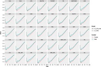
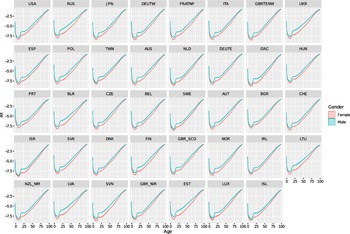
for all populations. These three figures provide some country-specific subplots in which the curves of the parameters are represented distinguishing by gender: the male population’s parameters are presented in blue, while the female population’s parameters are reported in red. The subplots are sorted in descending order with respect to the population size in the year 2000, the first year of the testing set. In each subplot, the solid lines refer to the LC_LCN_mse estimates while the dashed lines denote those obtained via LC_SVD. We discuss these figures one by one in the following.
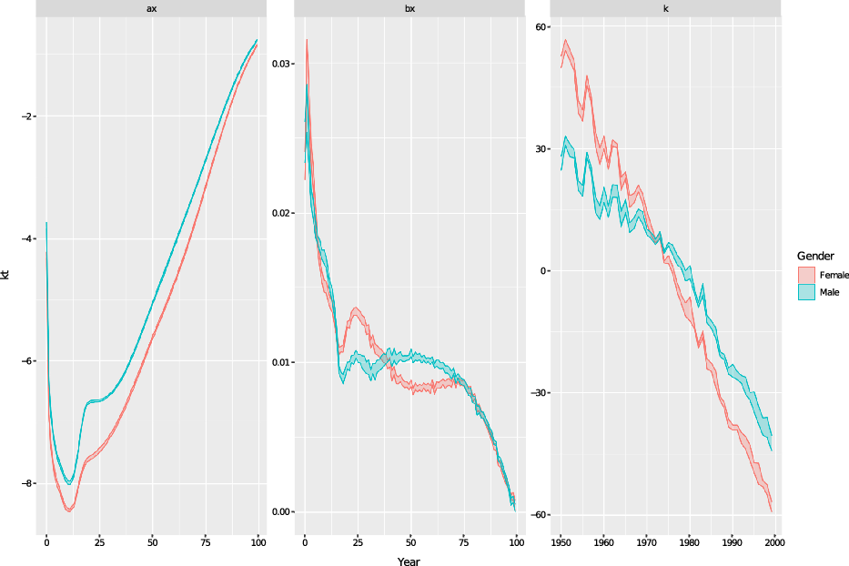
Comparison of the LC_LCN_mse and LC_SVD estimates of
 $\left(a_x^{(i)}\right)_{x \in \mathcal{X}}$
for all the populations considered; fitting period 1950–1999; countries are sorted by population size in 2000.

Comparison of the LC_LCN_mse and LC_SVD estimates of
 $\left(a_x^{(i)}\right)_{x \in \mathcal{X}}$
distinguishing by model; fitting period 1950–1999.

Comparison of the LC_LCN_mse and LC_SVD estimates of
 $\left(b_x^{(i)}\right)_{x \in \mathcal{X}}$
for all the populations considered; fitting period 1950–1999; countries are sorted by population size in 2000.

Comparison of the LC_LCN_mse and LC_SVD estimates of
 $\left(k_t^{(i)}\right)_{t \in \mathcal{T}}$
for all the populations considered; fitting period 1950–1999; countries are sorted by population size in 2000.

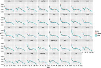
Figure 4 compares the estimations of the
 $\left(a_x^{(i)}\right)_x$
for all populations considered. First, we observe that all the curves present the classical life-table shape and the female curves are located below the male ones. Furthermore, since the dotted and solid lines seem almost coincide, we conclude that both approaches produce similar
 $a_x^{(i)}$
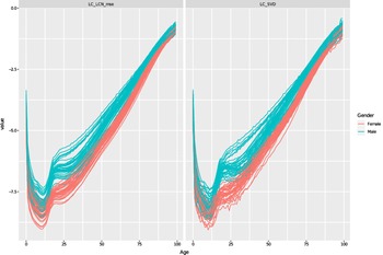
estimates. To better understand the differences between these estimations, we analyse them more closely by representing the
 $\left(a_x^{(i)}\right)_x$
curves simultaneously on the same plot. Figure 5 shows this comparison on two different subplots; the first one concerns the LC_SVD model (right) while the second one represents the LC_LCN_mse model (left). Looking at the
 $\left(a_x^{(i)}\right)_x$
estimations from this point of view, we observe that the LC_SVD curves present some erratic fluctuations while the LC_LCN_mse estimates appear to be smooth. This could due to the random fluctuations often present in the mortality data which also affect the parameters estimates. We could explain this evidence by arguing that the LC_SVD works on a population-specific subset of data, and then its estimates, could be more sensitive to the random fluctuations present in that data. On the contrary, the LC_LCN_mse model, which uses a large amount of data to fit and allows the information sharing among the populations through cross-population parameters, prevents population-specific overfitting and produces estimates less sensitive to these fluctuations.
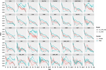
Figure 6 compares the
 $\left(b_x^{(i)}\right)_x$
estimates (individually scaled in [0, 1]). Here, we observe that the two approaches involve quite different
 $\left(b_x^{(i)}\right)_x$
estimations. This is especially evident for low-population countries, which are represented at the bottom of the figure. In particular, we note that the LC_SVD estimates appear to be smooth for high-population countries (e.g., USA and JPN) while they present irregular patterns for low-population countries (e.g., LUX and ISL). This evidence was already discussed in the literature; see Delwarde et al. (Reference Delwarde, Denuit and Eilers2007). Also in this case, this could be due to the random fluctuations present in the mortality rates, which appears more pronounced for low-population countries (Jarner and Kryger, Reference Jarner and Kryger2011). We believe this is related to the law of large numbers, which makes volatility in mortality rates larger for low-population countries. On the contrary, the LC_LCN_mse curves are quite smooth for all countries. This can be justified with the same arguments given for the
 $\left(a_x^{(i)}\right)_x$
estimates.
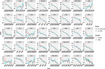
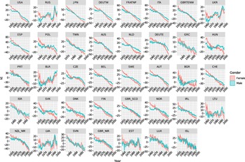
Figure 7 compares the LC_LCN_mse and LC_SVD estimates of
 $\left(k_t^{(i)}\right)_t$
for all populations considered. Overall, the estimates appear rather similar; however, one might notice that the LC_LCN_mse model, in some cases, presents
 $\left(k_t^{(i)}\right)_t$
series with more pronounced peaks than the classic LC_SVD model. This evidence is particularly visible in countries such as RUS (especially for females), UKR, POL, GRC, HUN, BLR (especially for females), BGR, LTU and LVA. It seems to suggest that the NN
 $k_t^{(i)}$
estimates are able to capture mortality fluctuations over time better, allowing a more appropriate measurement of the uncertainty when forecasting is involved.
5.2. Poisson loss minimisation
As emphasised in Section 2.1, the assumption of homoskedastic error structure, which follows the ordinary least squares estimation, often appears unrealistic. In this section, assuming a Poisson number of death
 $D^{(i)}_{x,t}$
, we explore the use of the Poisson loss function to train the NN models. In particular, we consider
 \begin{equation}D^{(i)}_{x,t} \sim Poisson \left(E^{(i)}_{x,t} e^{m^{(i)}_{x,t}}\right),\end{equation}
where
 \begin{equation*} {m}_{x,t}^{(i)} = \bigg( w^{(a)}_{x,0} + \left\langle \boldsymbol{w}_x^{(a)}, \boldsymbol{z}_{\mathcal{I}}^{(a)} \right\rangle \bigg)\ + \end{equation*}
 \begin{equation} + \bigg( w^{(b)}_{x,0} +\left\langle \boldsymbol{w}_x^{(b)}, \boldsymbol{z}_{\mathcal{I}}^{(b)} \right\rangle \bigg) \cdot \bigg( w^{(k_2)}_0 + \left\langle \boldsymbol{w}^{(k_2)}, \phi^{(k_1)} \bigg( \boldsymbol{w}^{(k_1)}_0 + W^{(k_1)} \log\!\left(\boldsymbol{m}_{t}^{(i)}\right) \bigg) \right\rangle \bigg).\end{equation}
In this setting, the NNs model fitting involves the minimisation of
 \begin{equation}L(\psi) = \sum_{x \in \mathcal{X}} \sum_{i \in \mathcal{I}}\sum_{t \in \mathcal{T}} \bigg( E^{(i)}_{x,t} e^{{m}_{x,t}^{(i)}}- D^{(i)}_{x,t} {m}_{x,t}^{(i)} \bigg) + c\\\end{equation}
which corresponds to maximise the log-likelihood function under the assumption (5.1) and
 $c \in \mathbb{R}$
. We use the same data of Section 5.1; however, this time we exclude the Canadian populations since there are several missing values in the data related to the exposure-to-risk and number of deaths. Here, we have
 $|\mathcal{I}| = 78$
.
The NN architectures previously selected are trained in the same setting: mortality experiences concerning calendar years in
 $\mathcal{T}_1$
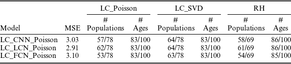
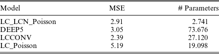
are used for training, the number of epochs was set equal to 2000, and the same training algorithm is employed. This time, the training sample contains 3498 examples since the 100 mortality experiences concerning Canadian populations are removed. The names of all the NN models are suitably modified by replacing “mse” with “Poisson.” The Keras code that defines the network architectures is provided in the Appendix C. In these experiments, we also included in the comparisons the ILC approach based on the Poisson maximum likelihood estimation (we refer to the results of this approach as LC_Poisson) and the results of individual Renshaw and Haberman (RH) models (Renshaw and Haberman, Reference Renshaw and Haberman2006). We estimate these two sets of models using the StMoMo R package. In particular, for the individual RH models, we observed that the fitting procedure for some populations does not converge. This result had already been highlighted in Perla et al. (Reference Perla, Richman, Scognamiglio and Wüthrich2021). Consequently, for the RH model, we report the results for 69 populations for which the fitting procedure was completed successfully. Again, we use the MSE between predicted mortality rates and the actual ones to measure the performance. Table 3 lists the forecasting MSE for each NN model and the number of populations and ages in which each network model beats the three benchmarks. The LC_SVD and the LC_Poisson. respectively obtain MSEs equal to
 $6.02 \times 10^{-4}$
and
 $5.19\times 10^{-4}$
(on 78 populations) while RH produces a MSE equal to
 $25.12\times 10^{-4}$
(on 69 populations).
Results of all three network architectures considered: forecasting MSEs, number of populations and ages in which each network beats the LC_Poisson, the LC_SVD and the RH models; forecasting period 2000–2018; MSEs values are in
 $10^{-4}$
.

First, we observe that all three NNs models overperform very well. In particular, the LC_LCN_Poisson produces the best performance, LC_CNN_Poisson is the second one and LC_FCN_Poisson is the least accurate. Comparing them against the benchmarks, we note that they overperform the LC_SVD, LC_Poisson and RH models in most of the populations and ages. Overall, we select the LC_LCN_Poisson model as the best model, and further comparisons against the benchmarks are provided below.
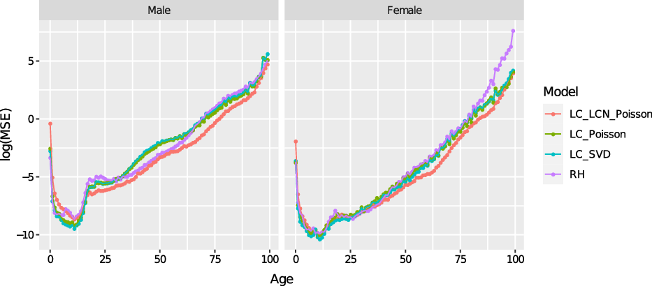
Figure 8 compares the LC_LCN_Poisson against the LC_SVD, LC_Poisson and RH models by analysing the error by age for both genders on a logarithmic scale. In all cases, the curves show the shape of a mortality table. Furthermore, we observe that, for both genders, the LC_LCN_Poisson model produces the lowest forecasting error for ages
 $x>20$
and this improvement is more evident for males. On the contrary, for ages
 $x\leq 20$
the LC_Poisson and the LC_SVD perform better.
Comparison error among the LC_LCN_Poisson, the LC_Poisson, the LC_SVD and the RH models for years in 2000–2018 for different ages and genders, MSE values are in
 $10^{-4}$
and on log-scale.

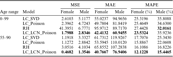
Table 4 reports the performances in terms of MSE, MAE (Mean Absolute Error) and MAPE (Mean Absolute Percentage Error) of these four models in the age ranges 0–99 and 55–90 for both genders in the 69 populations in which the RH model converges. The LC_LCN_Poisson model produces the best performance in all cases except for the MAPE on males aged 0–99. This is not surprising since the MAPE is the mean of the residuals (in absolute value) divided by the respective actual mortality rates. Therefore, they may be more sensitive to errors made on ages with low mortality rates. Indeed, as illustrated by Figure 8, the LC_LCN_Poisson model is less accurate for ages
 $x\leq 20$
where mortality rates are very small and there the global MAPE on the age range 0–99 results higher. On the contrary, it appears the best also from a MAPE perspective when the age range 55–90 is considered. Furthermore, Table 4 appears to confirm that the LC_LCN_Poisson model induces a more significant improvement for males.
MSE, MAE and MAPE of LC_SVD, LC_Poisson, RH and LC_LCN_Poisson in the age ranges 0–99 and 55–90 for each gender; MSE and MAE values are in
 $10^{-4}$
on the 69 populations in which the RH model converges; the best performance is reported in bold.

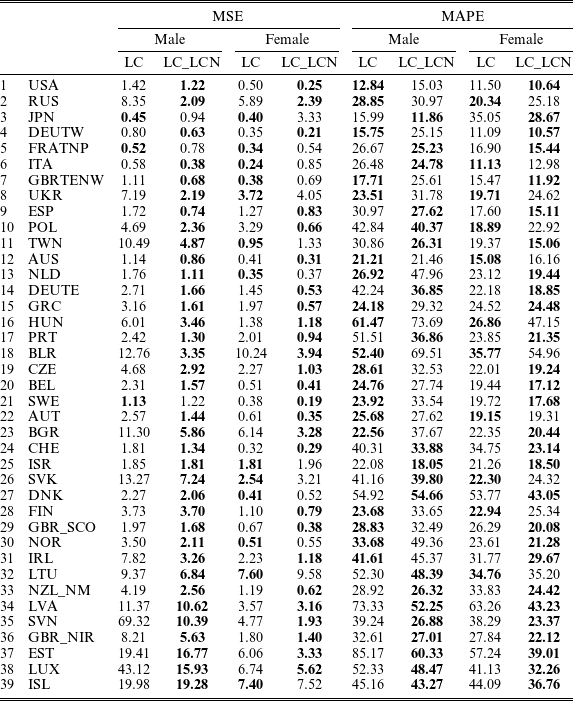
Table 5 reports the LC_LCN_Poisson and LC_Poisson models’ MSE and MAPE in all countries under investigation distinguishing by gender. The best performance in each population is reported in bold. From a MSE perspective, we observe that, in the most of the cases, LC_LCN_Poisson beats the LC_Poisson and this evidence appears especially evident for male populations. In addition, in some of these cases, the improvement produced by LC_LCN_Poisson model results quite large (see e.g., the male populations of LUX, SVN, SVK, BLG, UKR and others). Many of these countries are low-population countries since they are located in the bottom of Table 5. This evidence suggests that LC_LCN_Poisson model could improve the forecasting in low-population countries whose data are often affected by random fluctuations. On the contrary, in the cases in which the LC_Poisson model beats the LC_LCN_Poisson model, the difference is often quite limited; the only cases in which this difference appears significant are the female populations of JPN and LTU. Analysing the MAPEs, the superiority of the LC_LCN_Poisson over the LC_Poisson is less evident, the first model beats the second one only in 60% of the cases. This can be explained by arguing again that the MAPE is more sensitive to errors made in ages with low mortality rates such as the young ages where the LC_LCN_Poisson is less accurate. The LC_LCN_Poisson beats the LC_Poisson again in 60/78 populations considering the age range of 55–90. Also in the MAPE case, it is evident that the LC_LCN_Poisson produces better performances with respect to the LC_Poisson in several low-population countries such as NZL_NM, LVA, SVN, GBR_NIR, EST, LUX and ISL.
Forecasting MSEs of the LC_LCN_Poisson (LC_LCN) and the LC_Poisson (LC) models on different populations; forecasting period 2000–2018; MSEs values are in
 $10^{-4}$
; the best performance is reported in bold.

We conclude that the LC_LCN_Poisson model presents an overall forecasting performance higher than the other competitors.
Table 5 reports the LC_LCN_Poisson and LC_Poisson models’ MSE and MAPE in all countries under investigation distinguishing by gender. The best performance in each population is reported in bold. From a MSE perspective, we observe that, in most of the cases, LC_LCN_Poisson beats the LC_Poisson, and this evidence appears especially evident for male populations. In addition, in some of these cases, the improvement produced by LC_LCN_Poisson model results quite large (see e.g., the male populations of LUX, SVN, SVK, BLG, UKR and others). Many of these countries are low-population countries since they are located in the bottom of Table 5. This evidence suggests that LC_LCN_Poisson model could improve the forecasting in low-population countries whose data are often affected by random fluctuations. On the contrary, in the cases in which the LC_Poisson model beats the LC_LCN_Poisson model, the difference is often quite limited; the only cases in which this difference appears significant are the female populations of JPN and LTU. Analysing the MAPEs, the superiority of the LC_LCN_Poisson over the LC_Poisson is less evident; the first model beats the second one only in 60% of the cases. This can be explained by arguing again that the MAPE is more sensitive to errors made in ages with low mortality rates such as the young ages where the LC_LCN_Poisson is less accurate. The LC_LCN_Poisson beats the LC_Poisson again in 60/78 populations considering the age range of 55–90. Also, in the MAPE case, it is evident that the LC_LCN_Poisson produces better performances with respect to the LC_Poisson in several low-population countries such as NZL_NM, LVA, SVN, GBR_NIR, EST, LUX and ISL. These results suggest that the LC_LCN_Poisson model presents an overall forecasting performance higher than the other competitors.
We conclude this paragraph comparing the LC_LCN_Poisson and the LC_Poisson against other well-known NN models used for large-scale mortality forecasting. In particular, we consider the DEEP5 architecture proposed in Richman and Wüthrich (Reference Richman and Wüthrich2021) and the LCCONV model proposed by Perla et al. (Reference Perla, Richman, Scognamiglio and Wüthrich2021). Table 6 lists the forecasting MSE and the number of parameters for each NN model and the LC_Poisson model. We observe that the performance of the LC_LCN_Poisson is the second from a forecasting accuracy perspective: it is more accurate than the DEEP5 and LC_Poisson models but less accurate than the LCCONV model. However, the LC_LCN_Poisson is the most parsimonious model: it presents around
 $1/10$
of the weights of the LCCONV model,
 $1/25$
of the weights of the DEEP5 model and around
 $1/7$
of the LC_Poisson. In conclusion, the LC_LCN_Poisson model presents two important advantages. First, as discussed in Section 4, it is easy to understand as the network components can be interpreted. Second, the LC_LCN_Poisson model does not modify the time-series part of the LC model and it is therefore possible to derive interval estimates for the forecast mortality rates.
Forecasting MSEs of the LC_LCN_Poisson, DEEP5, LCCONV and LC_Poisson models on the 78 populations; forecasting period 2000–2018; MSEs values are in
 $10^{-4}$
.

5.3. Some sensitivity tests
In this section, the LC_LCN_Poisson model is submitted to some sensitivity checks. First, we analyse the sensitivity of the LC_LCN_Poisson model with respect to the set of populations considered
 $\mathcal{I}$
. The forecasting performance should not roughly change when a smaller set of populations is considered. To this aim, we split the full set of populations
 $\mathcal{I}$
into two subsets, the first one,
 $\mathcal{I}_{HP}$
, contains the male and female populations the 20 highest population countries (from 1-20 of Table 5) while the second set,
 $\mathcal{I}_{LP}$
, includes the male and female populations of the remaining 19 the lowest population countries such that
 $\mathcal{I} = \mathcal{I}_{LP} \cup \mathcal{I}_{HP}$
.
The model LC_LCN_Poisson model is run separately on these two sets, and the results have been collected in Table 7. Again, the results for the LC_SVD and LC_Poisson models are reported to make comparisons. We observe that in the high-population countries, all the models produce lower MSEs than that obtained on the full set
 $\mathcal{I}$
. On the contrary, we observe that the respective MSEs are significantly higher in the low-population countries. We note that the LC_LCN_Poisson model still overperforms the two benchmarks in both cases. Therefore, we conclude that the LC_LCN_Poisson model is competitive even when smaller populations are considered. Nevertheless, it is reasonable to believe that the LC_LCN_Poisson model benefits from using as much data as possible for the training.
Forecasting MSEs of the LC_LCN_Poisson, LC_Poisson, LC_SVD models on
 $\mathcal{I}_{HP}$
and
 $\mathcal{I}_{LP}$
; forecasting period 2000–2018; MSEs values are in
 $10^{-4}$
.

In the second part of this section, we investigate how much the LC_LCN_Poisson model’s results change in the different training attempts. As highlighted in Section 3, the results of training a NN are somewhat variable, and, therefore, the estimation of the optimal network parameters
 $\hat{\psi}$
can vary between training attempts. This also affects the NN estimations of the LC parameters which vary themselves between training attempts. In this section, we investigate the variability of these estimates keeping in mind that a small variability means that the results produced by the NN model are stable. On the contrary, a large variability could highlight that the results produced by the network change significantly between the different training attempts and then they are not stable. To investigate this point, we consider the NN estimations of the LC parameters obtained in the ten different training attempts of the LC_LCN_Poisson model. Figure 9 represents the full ranges of variation of the NN estimations of the LC parameters for the Italian populations. It includes three subplots which refer to the
 $\left(a_x^{(i)}\right)_x$
,
 $\left(b_x^{(i)}\right)_x$
and
 $\left(k_t^{(i)}\right)_t$
parameters respectively.
Variability in the estimates of
 $\left(a_x^{(i)}\right)_x$
,
 $\left(b_x^{(i)}\right)_x$
and
 $\left(k_t^{(i)}\right)_t$
obtained by the LC_LCN_Poisson model in 10 training attempts for Italian populations; fitting period 1950–1999.

Two lines are visualised for each parameter curve; the higher curve represents the maximum values observed in the different training attempts while the lower one represents the minimum values. Intuitively, the area between these two bounds is the range of observed values in the ten different runs. The graphical elements in blue refer to the male population’s parameters, while those in red refer to the female population’s ones. Overall, the estimates of the LC parameters obtained seem to vary not so much. First, we observe that the maximum and minimum values obtained for the parameters
 $a_x$
for the Italian populations are almost overlapped. This evidence means that the estimates obtained in the ten training attempts are almost identical. About the
 $\left(b_x^{(i)}\right)_{x}$
parameters, we note that the variability appears marginally greater than the other two parameters for the middle ages. Nonetheless, since the area between the two curves is very limited in these cases, we can conclude that the estimates obtained via the LC_LCN_Poisson model are stable. A similar evidence is visible in the
 $\left(k_t^{(i)}\right)_t$
estimates. It should be remarked that these graphs only consider the uncertainty due to network training.
In Appendix D, Figures D.1, D.2, D.3 extend this analysis to all the other populations. Figure D.1 depicts the ranges of the
 $(a^{(i)}_x)_x$
estimates for the different populations; Figures D.2 and D.3 analyse respectively the estimates
 $(b^{(i)}_x)_x$
and
 $(k^{(i)}_t)_t$
.
The findings obtained for the Italian populations appear to work for all other countries. The estimates obtained for the LC parameters
 $a^{(i)}_x$
and
 $k_t^{(i)}$
results are not very variable for all the populations considered. The estimates of the
 $b^{(i)}_x$
result more variables than the other parameters, especially for low-population countries. However, as shown in Figure D.2, the variability increases only for some ages and in a marginal way.
6. Conclusions
This paper proposes a NN approach for calibrating the ILC models of multiple populations. The parameters of the ILC models are jointly estimated through a NN that simultaneously processes the mortality data of all populations. In this way, each individual LC model is calibrated by exploiting all the available information instead of using a population-specific subset of data as in the traditional fitting approaches. We experiment with our approach on the HMD data considering different network architectures and loss functions, analysing the reasonableness of the parameters estimates and the resulting forecasting performance. From a forecasting perspective, the numerical results show that all the network models considered overperform the traditional LC_SVD, LC_Poisson, RH approach for a large set of populations. The best performance is obtained from the LC_LCN_Poisson model, which employs locally connected layers to extract features from the mortality rate curves. In particular, the forecasting performance of the LC_LCN_Poisson model results comparable to the DEEP5 model proposed in Richman and Wüthrich (Reference Richman and Wüthrich2021) and marginally poorer than the LCCONV model proposed Perla et al. (Reference Perla, Richman, Scognamiglio and Wüthrich2021). The LC_LCN_Poisson model, in addition, is very efficient from the number of parameters perspective presents two important advantages. First, it is easy to understand as the network components can be interpreted. Second, the LC_LCN_Poisson model does not modify the time-series part of the LC model, and it is possible to derive interval estimates for the forecast mortality rates. Numerical experiments also show that, differently from the traditional fitting schemes, our approach produces smoother estimates of the age-specific LC parameters curves. This result appears evident for the low-population countries in which the random fluctuations in mortality rates affect the LC_SVD and the LC_Poisson estimates. This could also be the case of annuity portfolios or pension funds’ data often collected considering small populations (Hunt and Blake, Reference Hunt and Blake2017). Interesting effects are also visible in the
 $k_t^{(i)}$
estimates which appear more flexible and able better to capture the variations of the population-specific mortality dynamics. This could allow a more appropriate measurement of the uncertainty when forecasting is involved. Furthermore, the numerical experiments performed in the paper also show that NN architectures based on linear and tanh activation overperform the ReLU networks similarly to Perla et al. (Reference Perla, Richman, Scognamiglio and Wüthrich2021). However, this result depends on the data and the best activation function could change when a different set of data is considered. In this sense, the NNs represent flexible modelling tools since they can analyse the data with linear and/or non-linear transformations. The activation function should be considered a hyper-parameter to choose on the basis of the data carefully. Future research will proceed in different directions. First, we intend to analyse the performance of the proposed model on other available data sources such as the (USMB) and insurance portfolio’s data. Second, we will investigate the use of NNs for fitting other stochastic mortality models. Both the single-population models belonging to the family of Generalised Age Period Cohort (GAPC) models (Villegas et al., Reference Villegas, Millossovich and Kaishev2018) and the multi-population extensions of the LC model such as Li–Lee (Li and Lee, Reference Li and Lee2005) and Kleinow (Reference Kleinow2015) models could be considered. Third, we aim to explore approaches to derive the confidence interval of the NN estimates LC parameters. Simulation-based techniques, such as bootstrap, would be difficult to apply in our setting since NN training is computationally expensive. A possible alternative would be to use the pinball loss function to train the NN as suggested in Richman (Reference Richman2021). Finally, we intend to explore the potential of the proposed large-scale mortality model in actuarial evaluations and longevity risk management.
Acknowledgements
The author thank the two anonymous referees whose comments helped to improve the manuscript.
Appendix A. Data details
List of selected countries in
 $\mathcal{R}$
with the respectively initial and final years considered.

Appendix B. Model specification for response variable in [0, 1]
Sometimes, machine learning models are developed defining the response variable scaled in [0, 1] by applying the MinMax scaling. In this case, the model in (4.6) can be rewritten as
 \begin{equation}\begin{split}\frac{\widehat{ \log\!({m}_{x,t}^{(i)})}- y_m}{y_M - y_m} = \boldsymbol{f}^{(a)} \left(\boldsymbol{z}_{\mathcal{I}}^{(a)}\right) + \boldsymbol{f}^{(b)} \left(\boldsymbol{z}_{\mathcal{I}}^{(b)}\right) \left(f^{(k_2)} \circ \boldsymbol{f}^{(k_1)}\right) \left(\log\!\left(\boldsymbol{m}_{t}^{(i)}\right)\right),\end{split}\end{equation}
where
 \[ y_m = \min_{{x \in \mathcal{X}, t \in \mathcal{T}_1, i \in \mathcal{I}}} \log\left(m_{x,t}^{(i)}\right) \quad \quad y_M = \max_{{x \in \mathcal{X}, t \in \mathcal{T}_1, i \in \mathcal{I}}} \log\left(m_{x,t}^{(i)}\right). \]
The network parameters are calibrated minimising the MSE between the scaled actual mortality rates and the predicted ones and the corresponding NN estimates of the LC parameters in the original scale can be computed as
 \begin{equation} \hat{a}_{x, NN}^{(i)} = \phi^{(a)} \bigg( \hat{w}_{x, 0}^{(a)}+\left\langle \hat{\boldsymbol{w}}_{x,\mathcal{R}}^{(a)}, \hat{\boldsymbol{z}}_{\mathcal{R}}^{(a)} (r) \right\rangle + \left\langle \hat{\boldsymbol{w}}_{x,\mathcal{G}}^{(a)} , \hat{\boldsymbol{z}}_{\mathcal{G}}^{(a)} (g) \right\rangle \bigg) \bigg(y_M - y_m\bigg) + y_m,\end{equation}
 \begin{equation} \hat{b}_{x, NN}^{(i)} = \phi^{(b)} \bigg( \hat{w}_{x, 0}^{(b)}+\left\langle \hat{\boldsymbol{w}}_{x,\mathcal{R}}^{(b)}, \hat{\boldsymbol{z}}_{\mathcal{R}}^{(b)} (r) \right\rangle + \left\langle \hat{\boldsymbol{w}}_{x,\mathcal{G}}^{(b)}, \hat{\boldsymbol{z}}_{\mathcal{G}}^{(b)} (g) \right\rangle \bigg),\end{equation}
 \begin{equation} \hat{k}_{t, NN}^{(i)} = \phi^{(k_2)} \bigg( \hat{w}^{(k_2)}_0 + \left\langle \hat{\boldsymbol{w}}^{(k_2)}, \phi^{(k_1)} \bigg( \hat{\boldsymbol{w}}^{(k_1)}_0 + \hat{W}^{(k_1)} \log\!\left(\boldsymbol{m}_{t}^{(i)}\right) \bigg) \right\rangle \bigg) \bigg(y_M - y_m\bigg).\end{equation}
Appendix C. Keras code of the neural network Models
In this section, we report the keras R code defining the NN architectures used. A brief description of the key variables is as follows.
The variable act controls the activation function
 $\phi^{(k_1)}$
of the
 $k_t^{(i)}$
-subnet. The activation of the
 $\boldsymbol{a}^{(i)}$
-subnet and
 $\boldsymbol{b}^{(i)}$
-subnet is set equal to the linear function but other alternatives could be considered as covered in the general framework provided in Section 4. The variable mod_type defines the architectures of the
 $k_t^{(i)}$
-subnet. It is possible to provide one of the following layers as hidden layer of the
 $k_t^{(i)}$
-subnet:
-
a fully connected layer when mod_type = ’FCN’,
-
a 1D locally connected layer when mod_type = ’LCN’,
-
a 1D convolutional layer when mod_type = ’CNN’.
The variable q_z controls the size of this hidden layer. For the FCN layer, it defines the number of units provided in the layer, while for the LCN and the CNN layers, it controls the size of the output through the stride and the kernel size G since
 $q_{{z_1}}=|\mathcal{X}|/G = 100/G$
.
Finally, the variable q_e controls the size of the embeddings
 $q_e = q^{(a)}_{\mathcal{R}} = q^{(a)}_{\mathcal{G}} = q^{(b)}_{\mathcal{R}} = q^{(b)}_{\mathcal{G}}$
in the first two subnets.
Listing 1: Keras code of the NN Models.

Appendix D. Robustness of the results
Variability in the
 $\left(a_x^{(i)}\right)_x$
estimates obtained by the LC_LCN_Poisson model in 10 training attempts for all the populations considered; fitting period 1950–1999; countries are sorted by population size in 2000.

Variability in the
 $\left(b_x^{(i)}\right)_x$
estimates obtained by the LC_LCN_Poisson model in 10 training attempts for all the populations considered; fitting period 1950–1999; countries are sorted by population size in 2000.

Variability in the
 $\left(k_t^{(i)}\right)_t$
estimates obtained by the LC_LCN_Poisson model in 10 training attempts for all the populations considered; fitting period 1950–1999; countries are sorted by population size in 2000.