1. Introduction
Gas–solid flows are encountered in industrial devices such as fluidized beds and in pneumatic conveying. It is generally agreed that the interaction of gas-phase velocity fluctuations with solid particles, as well as particle–particle interactions, play an important role in the formation of complex flow structures such as the core annular structure (Miller & Gidaspow Reference Miller and Gidaspow1992) that is observed in circulating fluidized beds. Gas-phase velocity fluctuations also affect gas–particle and particle–wall heat transfer, and the mixing of chemical species inside the fluidized bed. This motivates the current study which is focused on understanding the origin and mechanisms responsible for the generation of gas-phase velocity fluctuations in fluidized beds. Furthermore, quantification of the level of gas-phase velocity fluctuations in canonical gas–solid flows is an important step towards understanding and modelling gas–solid flow in industrial devices.
Device-scale calculations using computational fluid dynamics (CFD) simulations of multiphase flow are a promising route to inexpensive design and scale-up of industrial process equipment (Halvorsen, Guenther & O’Brien Reference Halvorsen, Guenther and O’Brien2003; Kashiwa & Gaffney Reference Kashiwa and Gaffney2003; Sun, Battaglia & Subramaniam Reference Sun, Battaglia and Subramaniam2007). CFD of multiphase flow involves solving the averaged equations for mass, momentum and energy in both the solid and fluid phases. In every grid cell, conservation equations for averaged quantities such as volume fraction and velocity are solved for both phases. These conservation equations are obtained using a statistical averaging procedure (Anderson & Jackson Reference Anderson and Jackson1967; Drew & Passman Reference Drew and Passman1998), and hence the solution to these averaged two-fluid equations involves modelling of the unclosed terms that represent interphase interactions.
The mean gas-phase velocity
 $\langle \boldsymbol{u}^{(\,f)}\rangle$
obtained by averaging the instantaneous momentum equation (Drew & Passman Reference Drew and Passman1998; Pai & Subramaniam Reference Pai and Subramaniam2009) evolves as
 $$\begin{eqnarray}\displaystyle & & \displaystyle \frac{\partial }{\partial t}\left\{{\it\rho}^{(f)}\left(1-{\it\phi}\right)\left\langle u_{i}^{(f)}\right\rangle \right\}+\frac{\partial }{\partial x_{j}}\left\{{\it\rho}^{(f)}\left(1-{\it\phi}\right)\left\langle u_{i}^{(f)}\right\rangle \left\langle u_{j}^{(f)}\right\rangle \right\}\nonumber\\ \displaystyle & & \displaystyle \quad =-\left(1-{\it\phi}\right)\left\langle g_{i}\right\rangle +\left\langle \frac{\partial I_{f}{\it\tau}_{ji}}{\partial x_{j}}\right\rangle \nonumber\\ \displaystyle & & \displaystyle \qquad -\,\frac{\partial }{\partial x_{j}}\left\{{\it\rho}^{(f)}\left\langle I_{f}u_{i}^{\prime \prime (f)}u_{j}^{\prime \prime (f)}\right\rangle \right\}-\left\langle {\it\tau}_{ji}n_{j}^{(p)}{\it\delta}\left(\boldsymbol{x}-\boldsymbol{x}^{(I)}\right)\right\rangle ,\end{eqnarray}$$
where
 $I_{f}\left(\boldsymbol{x},t\right)$
is the indicator function of the fluid (or gas) phase, which is unity if the point
 $\boldsymbol{x}$
lies in the fluid phase and zero otherwise. In this equation,
 $u_{i}^{\prime \prime (f)}=u_{i}-\langle u_{i}^{(\,f)}\rangle$
denotes the fluctuations in the fluid velocity field with respect to the phase-averaged fluid velocity,
 $\left(1-{\it\phi}\right)$
is the average volume fraction of the fluid phase,
 ${\it\rho}^{(f)}$
is the material density of the fluid phase,
 $\boldsymbol{n}^{(p)}$
is the unit normal vector pointing outward from the solid phase into the gas phase and
 ${\it\delta}(\boldsymbol{x}-\boldsymbol{x}^{(\boldsymbol{I})})$
is the Dirac delta function representing the gas–solid interface. In (1.1),
 $\boldsymbol{g}$
represents the body forces (hydrostatic pressure gradient, acceleration due to gravity, etc.) acting per unit volume of an infinitesimal fluid element, while
 ${\bf\tau}$
represents the surface stresses (both pressure and viscous stresses) acting on the surface of an infinitesimal fluid element. The first two terms on the right-hand side are the average body force density and the divergence of the average fluid-phase stress respectively. The last two unclosed terms that need to be modelled are the transport of fluid-phase velocity fluctuations (fluid-phase Reynolds stress) and the average interphase momentum transfer respectively. The average interphase momentum transfer
 $\langle {\it\tau}_{ji}n_{j}^{(p)}{\it\delta}\left(\boldsymbol{x}-\boldsymbol{x}^{(I)}\right)\rangle$
has been extensively studied and there is a general consensus on the closure models for this term (Ergun Reference Ergun1952; Wen & Yu Reference Wen and Yu1966; Syamlal & O’Brien Reference Syamlal and O’Brien1987; Gidaspow Reference Gidaspow1994; Hill, Koch & Ladd Reference Hill, Koch and Ladd2001a
,Reference Hill, Koch and Ladd
b
; van der Hoef, Beetstra & Kuipers Reference van der Hoef, Beetstra and Kuipers2005; Beetstra, van der Hoef & Kuipers Reference Beetstra, van der Hoef and Kuipers2007; Reddy et al.
Reference Reddy, Jin, Nandakumar, Minev and Joshi2010; Tenneti, Garg & Subramaniam Reference Tenneti, Garg and Subramaniam2011). However, the gas-phase Reynolds stress
 $\langle I_{f}u_{i}^{\prime \prime (f)}u_{j}^{\prime \prime (f)}\rangle$
has not been comprehensively quantified in the parameter range corresponding to fluidized beds. It should be noted that this pseudo-turbulent gas-phase velocity fluctuation is naturally incorporated in any particle-resolved direct numerical simulation (PR-DNS) of gas–solid flow that is used to derive the drag expression.
In the absence of such comprehensive quantification, the transport of the gas-phase Reynolds stress
 $R_{ij}^{(f)}=\langle I_{f}u_{i}^{\prime \prime (f)}u_{j}^{\prime \prime (f)}\rangle$
is sometimes neglected in CFD simulations of dense gas–solid flow on the grounds that the dominant forces in the gas-phase momentum balance are the pressure drop and the drag force. Similarly, due to the lack of data for
 $R_{ij}^{(f)}$
at low volume fractions, this term is also neglected in some CFD simulations of dilute gas–solid flow (Agrawal et al.
Reference Agrawal, Loezos, Syamlal and Sundaresan2001).
Nevertheless, there is evidence to indicate that gas-phase velocity fluctuations can be significant. Hot-wire measurements by Moran & Glicksman (Reference Moran and Glicksman2003) indicate that the level of gas-phase velocity fluctuations can be significant in a circulating fluidized bed riser at dilute solid volume fraction. Moreover, CFD simulations of dilute gas–solid flow based on the Reynolds-averaged Navier–Stokes (RANS) equations that incorporated a model for the transport of the gas-phase Reynolds stress generally showed better agreement for mean flow velocity profiles with experiments in particle-laden pipe flows (Bolio & Sinclair Reference Bolio and Sinclair1995; Bolio, Yasuna & Sinclair Reference Bolio, Yasuna and Sinclair1995; Crowe Reference Crowe2000; Zhang & Reese Reference Zhang and Reese2003). These observations, along with the measurements of Moran & Glicksman (Reference Moran and Glicksman2003), indicate that quantification and modelling of the gas-phase Reynolds stress over a range of solid volume fraction and mean slip Reynolds number (based on the mean slip velocity between the solid and gas phases) is necessary.
In industrial applications of gas–solids flow such as fluidized beds, the solid-to-fluid density ratio is of the order of 1000, and the particle diameter
 $d_{p}$
ranges from 50 to
 $500~{\rm\mu}\text{m}$
. Therefore particle inertia is significant. Furthermore, the particle diameter is usually larger than the Kolmogorov length scale
 ${\it\eta}$
. In such flows the mean slip velocity between the solid and the gas phase becomes an important parameter. The mean slip velocity causes an asymmetric pressure distribution around the particles and also results in the formation of boundary layers around the particle surface. The pressure asymmetry results in the formation of wake structures and contributes to gas-phase velocity fluctuations that interact with the particles downstream. These velocity fluctuations are generated in the gas phase even in ‘laminar’ gas–solid flows. They add to the inherent turbulent velocity fluctuations in the gas phase, and contribute significantly to the gas-phase Reynolds stress. In this paper, we denote local particle-scale gas-phase velocity fluctuations generated by the presence of particles as pseudo-turbulent velocity fluctuations, and the kinetic energy associated with these fluctuations is called the pseudo-turbulent kinetic energy (PTKE). Most closure models for the gas-phase Reynolds stress do not distinguish between the pseudo-turbulent and inherent turbulent velocity fluctuations in the flow. This is because both of these mechanisms essentially manifest themselves as a non-zero Reynolds stress in the gas phase. However, the length and time scales associated with the turbulent and pseudo-turbulent contributions can be different. Therefore, it is useful from a modelling viewpoint to distinguish pseudo-turbulence from the turbulent velocity fluctuations intrinsic to the gas phase in gas–solid suspensions. It should be noted that due to the nonlinearity of the Navier–Stokes equations, it is likely that although the mechanisms responsible for the generation of PTKE and inherent turbulence are different, their effect could be coupled.
The fluctuations in gas-phase velocity that contribute to the gas-phase Reynolds stress
 $R_{ij}^{(f)}$
arise from fluid motions over a range of length scales. In device-scale two-fluid RANS calculations, the closure model for
 $R_{ij}^{(f)}$
can be termed a macroscale closure that represents these fluid motions over the entire range of length scales. In a RANS closure, the PTKE contribution can be simply taken as additive to the closure for the turbulent contribution. Currently we are not aware of any evidence from particle-resolved simulations that validates the additive approach, or indicates the need for more sophisticated models. There are several reasons for this. One is that it is non-trivial to perform PR-DNS simulation of a homogeneous turbulent particle-laden flow where there is sustained inherent turbulence as well as PTKE, without artificially forcing the flow. While in single-phase turbulence one can force at large scales and simulate the natural dynamics of the energy cascade, current computational limitations do not permit the dynamic range needed to access this range of scales using PR-DNS. Furthermore, inertial particles dynamically interact with fluid eddies of a much larger scale, and it is well established that the presence of inertial particles modifies the fluid velocity spectra at large scales. In particle-laden flows, such artificial forcing can contaminate the natural dynamics of the system. An alternative to artificial forcing in single-phase turbulence is to perform homogeneous shear simulations to sustain the turbulence level. However, our analysis indicates that subjecting the fluid phase to linear shear does not ensure that the gas–solid flow will remain statistically homogeneous. In the absence of viable options to sustain inherent turbulence in current PR-DNS of homogeneous flows, it is difficult to arrive at a definitive conclusion on this point. Therefore, the simple additive approach is a first approximation that could be improved by using a weighted sum. This approach may by legitimate since in a RANS closure there is no distinction on the basis of length or time scales.
In large-eddy simulation (LES) of gas–solid flows (Capecelatro & Desjardins Reference Capecelatro and Desjardins2013), the gas-phase velocity is partitioned into resolved (meso) scales and unresolved (micro) scales that need to be modelled. The gas-phase momentum equation with no interphase mass transfer in such LES (Capecelatro & Desjardins Reference Capecelatro and Desjardins2013) reads
 $$\begin{eqnarray}\displaystyle & & \displaystyle \frac{\partial }{\partial t}\left({\it\rho}^{(f)}\left(1-{\it\phi}\right)\tilde{\boldsymbol{u}}^{(f)}\right)+\boldsymbol{{\rm\nabla}}\boldsymbol{\cdot }\left({\it\rho}^{(f)}\left(1-{\it\phi}\right)\tilde{\boldsymbol{u}}^{(f)}\tilde{\boldsymbol{u}}^{(f)}\right)\nonumber\\ \displaystyle & & \displaystyle \quad =\boldsymbol{{\rm\nabla}}\boldsymbol{\cdot }\left(\bar{{\bf\tau}}-\boldsymbol{R}_{u}\right)+\left(1-{\it\phi}\right){\it\rho}^{(f)}\boldsymbol{g}-\boldsymbol{F}^{inter},\end{eqnarray}$$
where
 $\tilde{\boldsymbol{u}}_{f}$
is the filtered gas-phase velocity,
 $\bar{{\bf\tau}}$
is the filtered viscous stress tensor,
 $\boldsymbol{R}_{u}=\left(1-{\it\phi}\right){\it\rho}^{(f)}\widetilde{\boldsymbol{u}^{\prime \prime }\boldsymbol{u}^{\prime \prime }}$
is the unresolved gas-phase Reynolds stress,
 $\boldsymbol{g}$
is the body force and
 $\boldsymbol{F}^{inter}$
is the interphase momentum transfer due to the drag force. If one considers an ensemble average of the term
 $\tilde{\boldsymbol{u}}^{(f)}\tilde{\boldsymbol{u}}^{(f)}$
, then this term contains
 $\langle \boldsymbol{u}^{(\,f)}\rangle \langle \boldsymbol{u}^{(\,f)}\rangle$
and the mesoscale portion of
 $R_{ij}^{(f)}$
. If the LES filter width is of the order of 10 particle diameters then the unresolved gas-phase Reynolds stress
 $\boldsymbol{R}_{u}$
is dominated by PTKE, which can be interpreted as the microscale contribution to
 $R_{ij}^{(f)}$
. It should be noted that, in general,
 $\boldsymbol{R}_{u}$
could contain microscale turbulent contributions if there is a mechanism to sustain them. Therefore, PTKE may account for only a portion of the
 $\boldsymbol{R}_{u}$
, rather than the entire contribution. However, the relative magnitude of these two contributions is not known in homogeneous particle-laden turbulent flow for the reasons already noted. A rough analysis based on single-phase turbulent scaling reveals that a relatively high turbulence Reynolds number
 $Re_{{\it\lambda}}$
is needed to generate inherent turbulent kinetic energy (TKE) that is comparable to the PTKE. Based on this reasoning, we believe that PTKE will be a dominant contributor to the fluid-phase velocity fluctuations at the microscale. Therefore, it is appropriate to use PR-DNS to quantify the PTKE and infer closure laws for these unresolved gas-phase velocity fluctuations
 $\boldsymbol{R}_{u}$
in LES. Such a closure may also be meaningfully interpreted as a closure for the microscale portion of
 $R_{ij}^{(f)}$
.
In most studies that employ gas–solid flow CFD using the two-fluid approach,
 $R_{ij}^{(f)}$
is modelled using an eddy viscosity (Ahmadi & Ma Reference Ahmadi and Ma1990b
; Bolio & Sinclair Reference Bolio and Sinclair1995; Balzer, Boelle & Simonin Reference Balzer, Boelle and Simonin1998; Benyahia, Syamlal & O’Brien Reference Benyahia, Syamlal and O’Brien2005) in a fashion similar to single-phase turbulence. The computation of the eddy viscosity in such an approach requires the knowledge of both the kinetic energy associated with the gas-phase velocity fluctuations
 $k^{(f)}$
and the dissipation rate
 ${\it\varepsilon}^{(f)}$
. In some works (Ahmadi & Ma Reference Ahmadi and Ma.1990a
,Reference Ahmadi and Ma
b
; Bolio & Sinclair Reference Bolio and Sinclair1995; Balzer et al.
Reference Balzer, Boelle and Simonin1998; Benyahia et al.
Reference Benyahia, Syamlal and O’Brien2005) a two-equation approach with transport equations for
 $k^{(f)}$
and
 ${\it\varepsilon}^{(f)}$
that are modified to account for the presence of solid particles is used to infer the eddy viscosity. There are also a few studies in which only a transport equation for
 $k^{(f)}$
is solved (one-equation approach), and
 ${\it\varepsilon}^{(f)}$
is modelled using single-phase turbulence models for the dissipation rate (Ahmadi & Ma Reference Ahmadi and Ma.1990a
,Reference Ahmadi and Ma
b
; Kenning & Crowe Reference Kenning and Crowe1997; Crowe Reference Crowe2000). A review of existing multiphase turbulence models can be found in Crowe, Troutt & Chung (Reference Crowe, Troutt and Chung1996). It is worthwhile to note that the algebraic models and the one-equation approaches require the quantification of
 $k^{(f)}$
as well as the dissipation rate
 ${\it\varepsilon}^{(f)}$
.
In dense gas–solid flows, non-intrusive measurements to quantify the level of gas-phase velocity fluctuations are difficult because of limited optical access, and the effect of intrusive instrumentation could alter the flow considerably. Therefore, simulations are a suitable alternative for quantifying gas-phase velocity fluctuations. A popular numerical approach that has been widely used to understand the effect of particles on the flow turbulence is the point-particle direct numerical simulation (PP-DNS) methodology (Squires & Eaton Reference Squires and Eaton1991; Elghobashi & Truesdell Reference Elghobashi and Truesdell1993; Boivin, Simonin & Squires Reference Boivin, Simonin and Squires1998; Sundaram & Collins Reference Sundaram and Collins1999; Mashayek & Taulbee Reference Mashayek and Taulbee2002; Calzavarini et al.
Reference Calzavarini, Volk, Bourgoin, Leveque, Pinton and Toschi2009). In PP-DNS, the particles are treated as point sources of momentum and the effect of the particles on the gas phase is represented by a force applied at the particle centre. This approach is valid only when the particle diameter
 $d_{p}$
is much smaller than the Kolmogorov length scale
 ${\it\eta}$
. However, as noted earlier, in industrial applications of gas–solid flow the particle diameter is usually larger than the Kolmogorov length scale (Moran & Glicksman Reference Moran and Glicksman2003).
When the particle size is larger than or comparable with the Kolmogorov length scale, it is important to resolve the boundary layers around the particle. In this regime, the appropriate numerical approach is the PR-DNS methodology in which all the scales of the inherent turbulence and the flow scales introduced by the presence of large particles are resolved. Particle-resolved direct numerical simulation has been used to study the interaction of a single particle with decaying (Bagchi & Balachandar Reference Bagchi and Balachandar2003; Burton & Eaton Reference Burton and Eaton2005) and stationary (Naso & Prosperetti Reference Naso and Prosperetti2010) isotropic turbulence. Particle-resolved direct numerical simulation has also been employed to study the effect of a collection of particles on decaying homogeneous isotropic turbulence (Lucci, Ferrante & Elghobashi Reference Lucci, Ferrante and Elghobashi2011; Subramaniam et al.
Reference Subramaniam, Mehrabadi, Horwitz and Mani2014), particle-laden turbulent channel flow (Uhlmann Reference Uhlmann2008; Kidanemariam et al.
Reference Kidanemariam, Chan-Braun, Doychev and Uhlmann2013) as well as gas–solid flow with upstream turbulence (Xu & Subramaniam Reference Xu and Subramaniam2010). This methodology has also been used to assess the ability of point-particle models in predicting particle acceleration when the Faxen correction is considered in the drag model for particle diameter
 $2\leqslant d_{p}/{\it\eta}\leqslant 14$
(Homann & Bec Reference Homann and Bec2010). It is worthwhile to note that an understanding of the generation of gas-phase velocity fluctuations using PR-DNS has been identified as one of the future directions in the review article by Balachandar & Eaton (Reference Balachandar and Eaton2010). Tenneti & Subramaniam (Reference Tenneti and Subramaniam2014) also argued that PR-DNS is a first-principles approach for developing accurate models for unclosed terms in statistical representations of multiphase flows, including kinetic theories of gas–solid flows (Garzo et al.
Reference Garzo, Tenneti, Subramaniam and Hrenya2012).
In this work, we use PR-DNS to quantify the level of gas-phase velocity fluctuations in flow through a statistically homogeneous fixed assembly of monodisperse spheres to determine the relative contribution of turbulent and pseudo-turbulent gas-phase velocity fluctuations to the steady level of
 $k^{(f)}$
. We first study the relaxation of gas-phase velocity fluctuations in initially turbulent gas–solid flow. We then focus on quantifying the steady PTKE in a laminar flow. We also quantify the dissipation rate of PTKE by considering the energy balance equation, in a manner similar to the work of Kenning & Crowe (Reference Kenning and Crowe1997). To differentiate between the pseudo-turbulent gas-phase velocity fluctuations and the inherent turbulence present in the flow field, we consider ‘laminar’ gas–solid flow to quantify the PTKE. In the context of this work, ‘laminar’ flow implies that there is no inherent turbulence in the flow field, i.e. in the absence of particles, the flow field is not turbulent.
In fixed-bed simulations the particles are held stationary and a steady flow is established by imposing a pressure gradient that corresponds to the desired flow rate. Use of the fixed-bed simulation set-up for gas–solid flow model development is justified on the grounds that the configuration of massive particles changes very slowly when compared with the time it takes to attain mean momentum balance (Hill et al.
Reference Hill, Koch and Ladd2001b
; Tenneti et al.
Reference Tenneti, Garg and Subramaniam2011). The fixed-bed simulation set-up has been successfully used to extract computational drag laws (Hill et al.
Reference Hill, Koch and Ladd2001a
,Reference Hill, Koch and Ladd
b
; van der Hoef et al.
Reference van der Hoef, Beetstra and Kuipers2005; Beetstra et al.
Reference Beetstra, van der Hoef and Kuipers2007; Tenneti et al.
Reference Tenneti, Garg and Subramaniam2011) as well as to understand the effect of particle clusters on gas-phase turbulence (Xu & Subramaniam Reference Xu and Subramaniam2010). Xu & Subramaniam (Reference Xu and Subramaniam2010) argued that the time scale over which the particle configuration changes depends on
 $Re_{T}=d_{p}T^{1/2}/{\it\nu}^{(f)}$
, which is the Reynolds number based on the particle fluctuating velocity characterized by the particle granular temperature
 $T=2k^{(p)}/3$
, where
 $k^{(p)}$
is the level of energy in solid-phase velocity fluctuations. Since both experiment (Cocco et al.
Reference Cocco, Shaffer, Hays, Reddy Karri and Knowlton2010) and PR-DNS (Tenneti et al.
Reference Tenneti, Garg, Hrenya, Fox and Subramaniam2010) of gas–solid flows show that
 $Re_{T}$
is low for high-Stokes-number suspensions, fixed particle assemblies have been used as a good approximation to freely evolving suspensions.
Recent PR-DNS of gas–solid flows (Uhlmann Reference Uhlmann2008; Xu & Subramaniam Reference Xu and Subramaniam2010) indicates that the gas-phase Reynolds stress is strongly anisotropic. In industrial gas–solid flows, the anisotropy of the velocity fluctuations results in anisotropic heat and scalar transport even in statistically homogeneous suspensions (Tenneti et al. Reference Tenneti, Sun, Garg and Subramaniam2013). This motivates us to quantify the level of anisotropy in gas–solid flows extracted from our PR-DNS data. These anisotropy results in conjunction with a model for gas-phase velocity fluctuations are used to propose an algebraic stress model (ASM) for the gas-phase Reynolds stress in gas–solid flows.
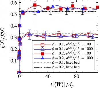
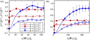
Although the assumption of fixed particle assemblies is a good approximation to freely moving particles with high Stokes number, in reality, however, particles move and collide freely in particle-laden flows. This may in turn affect the level of gas-phase velocity fluctuations. In order to account for these effects, we report PR-DNS of freely evolving homogeneous gas–solid suspensions with a finite mean slip velocity. Numerical simulations of freely evolving suspensions have been performed (Yin & Koch Reference Yin and Koch2007) to study the sedimentation of particles under gravity in the presence of fluid. In these studies, the steady mean flow Reynolds number attains a unique value that depends on the problem parameters (gas and particle densities, solid volume fraction, gravitational acceleration, etc.). Therefore, in sedimenting suspensions it is not possible to simulate arbitrary Reynolds numbers. However, the simulation of freely evolving suspensions in an accelerating frame of Tenneti et al. (Reference Tenneti, Garg, Hrenya, Fox and Subramaniam2010) enables us to simulate suspensions at arbitrary Reynolds numbers while maintaining other parameters at fixed values. Using this methodology, gas-phase velocity fluctuations of freely evolving suspensions are compared for selected problem parameters (
 $Re_{m}=20$
,
 ${\it\phi}=0.1$
and 0.2,
 ${\it\rho}^{(p)}/{\it\rho}^{(f)}=100$
and 1000) with data from fixed particle assemblies at the same solid volume fraction and Reynolds number that have not been previously reported to the best of our knowledge. This direct comparison gives us insight into the effect of freely moving particles on gas-phase velocity fluctuations. In addition, we verify the validity of the fixed-bed approximation to freely evolving suspensions of particles with high Stokes number.
The rest of the paper is organized as follows. In § 2 we define the ensemble-averaged quantities that are computed from PR-DNS. We then briefly describe our PR-DNS approach and its validation in §§ 3 and 4 respectively. The flow set-up is then described in detail in § 5. The evolution of an initially turbulent gas phase in steady mean flow through homogeneous particle assemblies is addressed in § 6. Then the results quantifying the level of PTKE in terms of solid volume fraction and mean slip Reynolds number are presented in § 7. Subsequently, in § 8 the anisotropy of the Reynolds stress is examined, and an ASM is proposed. We continue our discussion with gas-phase velocity fluctuations in freely evolving suspensions in § 9. Quantification of the dissipation is summarized in § 10, followed by conclusions in § 11.
2. Gas-phase velocity variance
In the Eulerian two-fluid theory the fluid-phase Reynolds stress is defined as a phasic average, which is an average conditional on the presence of the fluid phase (Drew Reference Drew1983; Drew & Passman Reference Drew and Passman1998; Pai & Subramaniam Reference Pai and Subramaniam2009). If
 $Q\left(\boldsymbol{x},t\right)$
is any field, then its phasic average
 $\langle Q^{(f)}\rangle \left(\boldsymbol{x},t\right)$
, referred to as its fluid-phase mean, is defined as
 $$\begin{eqnarray}\left\langle Q^{(f)}\right\rangle \left(\boldsymbol{x},t\right)=\frac{\left\langle I_{f}\left(\boldsymbol{x},t\right)Q\left(\boldsymbol{x},t\right)\right\rangle }{\left\langle I_{f}\left(\boldsymbol{x},t\right)\right\rangle },\end{eqnarray}$$
where
 $I_{f}$
is the fluid-phase indicator function defined in § 1.
Using this definition, the ensemble-averaged kinetic energy in the fluid phase
 $\langle E^{(f)}\rangle$
is defined as
 $$\begin{eqnarray}\left\langle E^{(f)}\right\rangle =\frac{1}{2}\frac{\left\langle I_{f}u_{i}u_{i}\right\rangle }{\left\langle I_{f}\right\rangle },\end{eqnarray}$$
where
 $\boldsymbol{u}$
is the fluid velocity. It is easy to see that the average kinetic energy in the fluid phase is the sum of the kinetic energy in the mean fluid motion
 $\bar{E}^{(f)}$
and the average kinetic energy in the fluctuating motions
 $k^{(f)}$
. The average kinetic energy in the mean fluid motion is given by
 $\bar{E}^{(f)}=(\langle u_{i}^{(f)}\rangle \langle u_{i}^{(f)}\rangle )/2$
, where the quantity
 $\langle u_{i}^{(\,f)}\rangle$
is the phase-averaged fluid velocity. The average kinetic energy in the fluctuating motion of the fluid is given by
 $$\begin{eqnarray}k^{(f)}=\frac{1}{2}\frac{\langle I_{f}u_{i}^{\prime \prime (f)}u_{i}^{\prime \prime (f)}\rangle }{\langle I_{f}\rangle },\end{eqnarray}$$
where fluctuations in the fluid velocity field are defined with respect to the phase-averaged fluid velocity, i.e.
 $u_{i}^{\prime \prime (f)}=u_{i}-\langle u_{i}^{(\,f)}\rangle$
. We now describe the procedure to compute
 $k^{(f)}$
from the solution of the flow past statistically homogeneous suspensions using PR-DNS.
2.1. Quantifying gas-phase velocity variance from PR-DNS
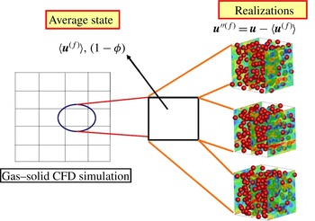
In PR-DNS, a single realization from the ensemble of events that contribute to the phasic average in (2.3) is simulated (cf. figure 1). The set
 $\{\boldsymbol{X}^{(i)},\boldsymbol{V}^{(i)},i=1,\dots ,N_{p}\}$
denotes the positions and velocities of a random configuration of
 $N_{p}$
particles that represents a realization
 ${\it\omega}$
of gas–solid flow in the event space
 ${\it\Omega}$
. Let
 $\boldsymbol{u}\left(\boldsymbol{x},t;{\it\omega}\right)$
be the fluid velocity field obtained from PR-DNS of flow past this configuration of particles. The ensemble-averaged fluid-phase velocity field is defined as (Subramaniam Reference Subramaniam2000)
 $$\begin{eqnarray}\left\langle \boldsymbol{u}^{(f)}\right\rangle \left(\boldsymbol{x},t\right)\equiv \int _{{\it\Omega}}I_{f}\left(\boldsymbol{x},t;{\it\omega}\right)\boldsymbol{u}\left(\boldsymbol{x},t;{\it\omega}\right)\text{d}P_{{\it\omega}},\end{eqnarray}$$
where
 $P_{{\it\omega}}$
is the probability measure that is defined on
 ${\it\Omega}$
. This concept is explained schematically in figure 1. The average gas-phase velocity and volume fraction that are solved in the CFD calculations are obtained by averaging over all possible realizations. Fluctuations in the gas-phase velocity are defined as departures of the instantaneous velocity field from the average gas-phase velocity.
Schematic showing the concept of the average fluid-phase velocity. The average fluid-phase velocity that is solved in gas–solid CFD simulations is obtained by averaging over all possible realizations.

If the flow is statistically homogeneous, ensemble-averaged quantities can be approximated by taking the volumetric mean of the solution fields, e.g. the volumetric mean of the velocity field over the fluid region is defined as
 $$\begin{eqnarray}\left\langle \boldsymbol{u}^{(f)}\right\rangle _{\mathscr{V}}\left(t;{\it\omega}\right)=\frac{1}{V^{(f)}}\int _{\mathscr{V}}I_{f}\left(\boldsymbol{x},t;{\it\omega}\right)\boldsymbol{u}\left(\boldsymbol{x},t;{\it\omega}\right)\text{d}V,\end{eqnarray}$$
where
 $V^{(f)}$
is the volume of the region occupied by the fluid phase. It has been shown by Tenneti et al. (Reference Tenneti, Garg and Subramaniam2011) that a statistically homogeneous gas–solid flow is well approximated by flow past a random configuration of particles in a periodically repeating unit cell. Therefore, volume averages are used here to estimate the true mathematical expectation. The volumetric mean approaches the ensemble average in the limit of infinite box size (i.e.
 $V\rightarrow \infty$
). Periodic boundary conditions can be used in a computational domain with finite box size provided that the two-point correlations in the particle and the fluid phases decay to zero within the box length. This is simply the two-phase extension of the criterion given by Pope (Reference Pope2000) for single-phase turbulent flows. Later, we show that the Eulerian two-point correlation of fluid velocity does indeed decay to zero within three to four particle diameters for different grid resolutions, box sizes and Reynolds numbers. However, a box of finite length does not completely account for the statistical variability arising from different particle configurations. In order to estimate the ensemble-averaged quantities from finite box sizes more accurately, we simulate fixed particle assemblies and average over different configurations. For fixed particle assemblies, the ensemble average is estimated by averaging over different configurations or realizations, i.e.
 $$\begin{eqnarray}\left\{\boldsymbol{u}^{(f)}\right\}_{\mathscr{V},\mathscr{M}}\left(t\right)=\frac{1}{\mathscr{M}}\mathop{\sum }_{{\it\mu}=1}^{\mathscr{M}}\left\langle \boldsymbol{u}^{(f)}\right\rangle _{\mathscr{V}}\left(t;{\it\omega}_{{\it\mu}}\right).\end{eqnarray}$$
In the above equation
 $\{\boldsymbol{u}^{(f)}\}_{\mathscr{V},\mathscr{M}}$
denotes an estimate to the true expectation
 $\langle \boldsymbol{u}^{(f)}\rangle$
and
 $\mathscr{M}$
denotes the number of independent realizations. Similarly, for each realization of the gas–solid flow we compute the kinetic energy in the fluctuating motions using volume averaging:
 $$\begin{eqnarray}k_{{\it\mu}}^{(f)}=\frac{1}{V^{(f)}}\int _{\mathscr{V}_{{\it\mu}}^{(f)}}\frac{1}{2}\left(\boldsymbol{u}(\boldsymbol{x},t,{\it\omega}_{{\it\mu}})-\left\{\boldsymbol{u}^{(f)}\right\}_{\mathscr{V},\mathscr{M}}\right)\boldsymbol{\cdot }\left(\boldsymbol{u}(\boldsymbol{x},t,{\it\omega}_{{\it\mu}})-\left\{\boldsymbol{u}^{(f)}\right\}_{\mathscr{V},\mathscr{M}}\right)\!\text{d}V.\end{eqnarray}$$
The value of
 $k_{{\it\mu}}^{(f)}$
obtained from a single realization (cf. (2.7)) is averaged over multiple independent simulations (MIS) to obtain an estimate for the ensemble-averaged kinetic energy
 $k^{(f)}$
:
 $$\begin{eqnarray}k^{(f)}=\frac{1}{\mathscr{M}}\mathop{\sum }_{{\it\mu}=1}^{\mathscr{M}}k_{{\it\mu}}^{(f)}.\end{eqnarray}$$
A similar approach is used to calculate the gas-phase Reynolds stress tensor
 $R_{ij}^{(f)}$
in § 8. In the next section, we describe the PR-DNS approach that is used in this work to quantify
 $k^{(f)}$
in steady flow past both fixed assemblies of spheres and freely evolving suspensions.
3. Numerical method
Several numerical methods have been developed for PR-DNS of gas–solid suspensions (Johnson & Tezduyar Reference Johnson and Tezduyar1997; Prosperetti & Oguz Reference Prosperetti and Oguz2001; Peskin Reference Peskin2002). The PR-DNS methodology employed in this work is called the particle-resolved uncontaminated-fluid reconcilable immersed boundary method (PUReIBM).
In PUReIBM, the entire physical domain is discretized using a uniform Cartesian grid and the governing equations of fluid flow are solved on all the grid points (including those lying inside the particles). The governing equations that are solved in PUReIBM are the continuity equation
 $$\begin{eqnarray}\boldsymbol{{\rm\nabla}}\boldsymbol{\cdot }\boldsymbol{u}=0\end{eqnarray}$$
and the Navier–Stokes equations
 $$\begin{eqnarray}{\it\rho}^{(f)}\frac{\partial \boldsymbol{u}}{\partial t}+{\it\rho}^{(f)}\boldsymbol{S}=-\boldsymbol{g}_{\mathit{IBM}}+{\it\mu}^{(f)}{\rm\nabla}^{2}\boldsymbol{u}+\boldsymbol{f}-{\it\rho}^{(f)}\boldsymbol{A}_{f}.\end{eqnarray}$$
Here,
 $\boldsymbol{u}$
is the instantaneous velocity field,
 $\boldsymbol{S}=\boldsymbol{{\rm\nabla}}\boldsymbol{\cdot }\left(\boldsymbol{u}\boldsymbol{u}\right)$
is the convective term in conservative form,
 $\boldsymbol{g}_{IBM}$
is the pressure gradient and
 $\boldsymbol{A}_{f}$
accounts for the acceleration of the frame of reference (Tenneti et al.
Reference Tenneti, Garg, Hrenya, Fox and Subramaniam2010). The simulation of a freely evolving suspension in PUReIBM is carried out in an accelerating frame of reference that moves with the mean velocity of the particles. The formulation of PUReIBM in an accelerating frame of reference enables the simulation of not just sedimenting suspensions, but arbitrary mean slip values, while maintaining average particle motion at rest in the accelerating frame. In other words, the use of an accelerating frame of reference facilitates examination of the influence of each flow parameter while maintaining other parameters constant.
The no-slip and no-penetration conditions on the fluid velocity at the particle surfaces are imposed via the additional immersed boundary (IB) force term
 $\boldsymbol{f}$
in (3.2). The full details of the computation of the IB force can be found in the work of Tenneti et al. (Reference Tenneti, Garg and Subramaniam2011). To compute the IB force, the surface of the sphere is represented by a discrete number of points called the boundary points that are parametrized in spherical coordinates. Two additional sets of points, termed as exterior and interior points, are generated by projecting the boundary points onto spheres of radii
 $r+{\rm\Delta}r$
and
 $r-{\rm\Delta}r$
respectively, with
 ${\rm\Delta}r$
chosen to be equal to the grid spacing. In PUReIBM, the IB force is computed at the interior points so that a desired velocity
 $\boldsymbol{u}^{(k,d)}$
is obtained at the
 $k\text{th}$
interior point. Following the direct forcing method proposed by Mohd-Yusof (Reference Mohd-Yusof1996) the IB force
 $\boldsymbol{f}^{(k)}$
at the
 $k\text{th}$
interior point is specified to cancel the remaining terms in the momentum conservation, and to force the velocity to its desired value
 $\boldsymbol{u}^{(k,d)}$
:
 $$\begin{eqnarray}\boldsymbol{f}^{(k)}={\it\rho}^{(f)}\frac{\boldsymbol{u}^{(k,d)}-\boldsymbol{u}^{(k,n)}}{{\rm\Delta}t}+{\it\rho}^{(f)}\boldsymbol{S}^{(k,n)}+\boldsymbol{g}_{\mathit{IBM}}^{(k,n)}-{\it\mu}^{(f)}{\rm\nabla}^{2}\boldsymbol{u}^{(k,n)}+{\it\rho}^{(f)}\boldsymbol{A}_{f}.\end{eqnarray}$$
It should be noted that all the terms in the above equation are evaluated at the
 $k\text{th}$
interior point. The desired velocity
 $\boldsymbol{u}^{(k,d)}$
depends on the velocity of the particle. For instance, for a fixed particle the desired velocity at the interior point is equal in magnitude but opposite in direction to the fluid velocity at the corresponding exterior point, so that the velocity at the boundary point is zero. The IB force so computed at all the interior points is interpolated to the neighbouring grid nodes that do not include those lying in the fluid phase to obtain
 $\boldsymbol{f}$
.
The governing equations in PUReIBM are solved in terms of fluctuating variables, and periodicity conditions are imposed on the appropriate fluctuating fields. The velocity field is decomposed into a spatially uniform mean flow
 $\langle \boldsymbol{u}\rangle _{\mathscr{V}}\left(t\right)$
and a fluctuating velocity field
 $\boldsymbol{u}^{\prime }$
, i.e.
 $$\begin{eqnarray}\boldsymbol{u}\left(\boldsymbol{x},t\right)=\left\langle \boldsymbol{u}\right\rangle _{\mathscr{V}}\left(t\right)+\boldsymbol{u}^{\prime }\left(\boldsymbol{x},t\right)\!,\end{eqnarray}$$
where the volumetric mean velocity is obtained by averaging the velocity field over the entire computational domain. Similar decompositions are written for the convective term
 $\boldsymbol{S}$
, pressure gradient
 $\boldsymbol{g}$
and IB forcing
 $\boldsymbol{f}$
terms. Substitution of the above decompositions in (3.1) and (3.2), followed by averaging over the entire computational domain, yields the volume-averaged mass and momentum conservation equations (detailed equations are given by Tenneti et al.
Reference Tenneti, Garg and Subramaniam2011). Evolution equations for the fluctuating variables are derived by subtracting the volume-averaged equations from their instantaneous counterparts. The resulting equations for the fluctuating variables are solved using a pseudo-spectral method, with the Crank–Nicolson scheme for the viscous terms, and an Adams–Bashforth scheme for the convective terms. A fractional time-stepping method that is based on Kim and Moin’s approach (Kim & Moin Reference Kim and Moin1985) is used to advance the fluctuating velocity fields in time.
In the case of fixed assemblies, the no-slip and no-penetration boundary conditions on
 $\boldsymbol{u}$
are imposed at the fixed particle surfaces. For a freely evolving suspension, the particles in PUReIBM move under the influence of hydrodynamic and collisional forces, and are represented in a Lagrangian frame of reference at time
 $t$
by
 $\{\boldsymbol{X}^{(i)}(t),\boldsymbol{V}^{(i)}(t)\;i=1\dots \,N_{p}\}$
, with
 $\boldsymbol{X}^{(i)}(t)$
and
 $\boldsymbol{V}^{(i)}(t)$
being the position and velocity of the
 $i$
th particle respectively and
 $N_{p}$
being the total number of particles. The position and translational velocity of the
 $i$
th particle evolve according to Newton’s second law as
 $$\begin{eqnarray}\displaystyle & \displaystyle \frac{\text{d}\boldsymbol{X}^{(i)}(t)}{\text{d}t}=\boldsymbol{V}^{(i)}(t), & \displaystyle\end{eqnarray}$$
 $$\begin{eqnarray}\displaystyle & \displaystyle m\frac{\text{d}\boldsymbol{V}^{(i)}(t)}{\text{d}t}=\boldsymbol{B}+\boldsymbol{F}_{h}^{(i)}(t)+\mathop{\sum }_{j=1\atop j\neq i}^{N_{p}}\boldsymbol{F}_{ij}^{(c)}(t), & \displaystyle\end{eqnarray}$$
 $\boldsymbol{B}$
is any external body force,
 $\boldsymbol{F}_{h}^{(i)}$
is the hydrodynamic force (calculated from the velocity and pressure fields at the particle surface) and
 $\boldsymbol{F}_{ij}^{(c)}$
is the contact force on the
 $i$
th particle as a result of collision with the
 $j$
th particle. Particle–particle interactions are treated using a soft-sphere model originally proposed by Cundall & Strack (Reference Cundall and Strack1979). In the soft-sphere approach, the contact mechanics between two overlapping particles is modelled by a system of springs and dashpots in both normal and tangential directions. The spring causes colliding particles to rebound and the dashpot mimics the dissipation of kinetic energy due to inelastic collisions. The spring stiffness coefficients in the tangential and normal directions are
 $k_{t}$
and
 $k_{n}$
respectively. Similarly, the dashpot damping coefficients in the tangential and normal directions are
 ${\it\eta}_{t}$
and
 ${\it\eta}_{n}$
respectively. The spring stiffness and dashpot damping coefficients are related to the coefficient of restitution and the coefficient of friction (Garg et al.
Reference Garg, Galvin, Li and Pannala2010a
).
The particles considered in this study are assumed to be frictionless. This implies that the tangential component of the contact force is zero, and thus rotation of particles is not accounted for in this study. Therefore, only the normal component of the contact force
 $\boldsymbol{F}_{\boldsymbol{n}_{ij}}$
is considered at time
 $t$
, and it is given by
 $$\begin{eqnarray}\boldsymbol{F}_{n_{ij}}=k_{n}{\it\delta}_{ij}\boldsymbol{n}_{ij}-\frac{m}{2}{\it\eta}_{n}\boldsymbol{V}_{n_{ij}},\end{eqnarray}$$
where
 ${\it\delta}_{ij}$
is the overlap between the particles computed using the relation
 $$\begin{eqnarray}{\it\delta}_{ij}=d_{p}-|\boldsymbol{X}^{(i)}-\boldsymbol{X}^{(j)}|\end{eqnarray}$$
and
 $\boldsymbol{V}_{n_{ij}}$
is the relative velocity in the normal direction which is defined using
 $$\begin{eqnarray}\boldsymbol{V}_{n_{ij}}=\left[\left(\boldsymbol{V}^{(i)}-\boldsymbol{V}^{(j)}\right)\boldsymbol{\cdot }\hat{\boldsymbol{r}}_{ij}\right]\hat{\boldsymbol{r}}_{ij}.\end{eqnarray}$$
The normal vector
 $\hat{\boldsymbol{r}}_{ij}$
is the unit vector along the line of contact pointing from particle
 $i$
to particle
 $j$
. The hydrodynamic and contact forces computed at each time step are then used to evolve the position and translational velocity of particles by (3.5) and (3.6) respectively.
The salient feature that distinguishes PUReIBM from other IB method approaches (including the original implementation of Mohd-Yusof Reference Mohd-Yusof1996) is that the IB forcing is restricted to those grid points that lie in the solid. Consequently, the velocity and pressure fields in the fluid phase are a solution to the unmodified Navier–Stokes equations with the appropriate boundary conditions. Since a flow field that is contaminated by additional forcing affects the calculation of
 $k^{(f)}$
and its dissipation rate, the uncontaminated flow field of PUReIBM is better suited for quantification of
 $k^{(f)}$
and its dissipation rate. Another consequence of the non-contamination of the fluid flow solution by the IB forcing is that the evolution equation of the volume-averaged fluid velocity exactly corresponds to that of the ensemble-averaged fluid-phase velocity. Therefore, it is possible to reconcile the solution obtained from PR-DNS with any random field theory of multiphase flow.
4. Validation
The PUReIBM PR-DNS methodology has been extensively validated (Garg et al. Reference Garg, Tenneti, Mohd-Yusof, Subramaniam, Pannala, Syamlal and O’Brien2010b ; Tenneti et al. Reference Tenneti, Garg and Subramaniam2011) by comparing the drag force obtained from PUReIBM with available experimental and simulation data in the literature in the following comprehensive suite of test cases.
-
(a) The drag acting on a single sphere (Garg Reference Garg2009; Garg et al. Reference Garg, Tenneti, Mohd-Yusof, Subramaniam, Pannala, Syamlal and O’Brien2010b ) with the experimental correlation of Schiller & Naumann (Reference Schiller and Naumann1935).
-
(b) The drag acting on simple cubic (SC) and face-centred cubic (FCC) arrangements (Tenneti et al. Reference Tenneti, Garg and Subramaniam2011) of particles in the Stokes flow regime with the results reported by Zick & Homsy (Reference Zick and Homsy1982) using the boundary integral method (semi-analytic solution).
-
(c) The drag acting on SC and FCC arrangements (Tenneti et al. Reference Tenneti, Garg and Subramaniam2011) of particles at moderate Reynolds numbers with the results published by Hill et al. (Reference Hill, Koch and Ladd2001b ) using the lattice Boltzmann method (LBM).
-
(d) The mean drag acting on a random arrangement (Tenneti et al. Reference Tenneti, Garg and Subramaniam2011) of particles in the Stokes flow regime with the results published by Hill et al. (Reference Hill, Koch and Ladd2001a ) and van der Hoef et al. (Reference van der Hoef, Beetstra and Kuipers2005) using the LBM.
-
(e) High-Reynolds-number flow past random arrays of monodisperse spheres with the ANSYS-FLUENT CFD package.
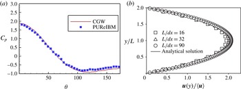
In addition to the comprehensive validation of the PUReIBM method (Garg et al. Reference Garg, Tenneti, Mohd-Yusof, Subramaniam, Pannala, Syamlal and O’Brien2010b ; Tenneti et al. Reference Tenneti, Garg and Subramaniam2011), we present selected additional validation tests to establish the numerical convergence and accuracy of PUReIBM near solid boundaries in figure 2. Figure 2(a) shows a comparison of the pressure coefficient along the surface of a sphere obtained from our PR-DNS with that reported by Clift, Grace & Weber (Reference Clift, Grace and Weber1978) (CGW) for an isolated sphere at a Reynolds number of 10. Figure 2(a) shows an excellent agreement of the coefficient of pressure profile on the surface of the sphere with the data reported in CGW. Figure 2(b) shows a comparison of the velocity field in a square duct at a Reynolds number of 20 with the analytical solution given by Cornish (Reference Cornish1928). We can see that the velocity profile obtained from PUReIBM is numerically converged and accurate. These plots show that in addition to computing the total drag accurately, our method also computes the correct contributions of pressure and viscous drag forces. In the following section we describe the simulation set-up used to compute the level of gas-phase velocity fluctuations and also discuss the choice of the numerical parameters needed to ensure numerically converged results.
(a) Variation of the coefficient of pressure
 $C_{p}$
along the surface of the sphere. The symbols are the data obtained from PUReIBM simulations for a Reynolds number of 10 while the solid line is that reported in the book authored by Clift, Grace and Weber (CGW) (Clift et al.
Reference Clift, Grace and Weber1978). (b) Comparison of the velocity profile in a square duct obtained from PUReIBM simulations at a Reynolds number of 20 with the analytical solution (Cornish Reference Cornish1928). It should be noted that the walls are generated using the IB method.

5. Simulation set-up
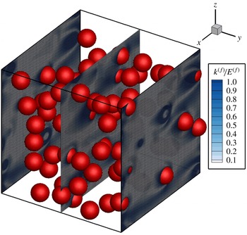
In our simulation set-up the particles are held stationary and a steady flow is established by imposing a pressure gradient that corresponds to the desired mean slip Reynolds number. A typical simulation of flow past a random arrangement of particles with contours of local kinetic energy
 $({u_{i}^{\prime \prime }}^{(f)}{u_{i}^{\prime \prime }}^{(f)})/2$
normalized by the mean energy is shown in figure 3. In all the simulations the mean flow is directed along the positive
 $x$
-axis.
For flow past homogeneous particle assemblies, a Reynolds number based on the magnitude of the mean slip velocity between the two phases is defined as
 $$\begin{eqnarray}\mathit{Re}_{m}=\left(1-{\it\phi}\right)\frac{\left|\left\langle \boldsymbol{W}\right\rangle \right|\,d_{p}}{{\it\nu}^{(f)}},\end{eqnarray}$$
where
 $|\langle \boldsymbol{W}\rangle |$
is the magnitude of the mean slip velocity,
 $d_{p}$
is the particle diameter and
 ${\it\phi}$
is the solid volume fraction. The mean slip velocity
 $\langle \boldsymbol{W}\rangle =\langle \boldsymbol{u}^{(p)}\rangle -\langle \boldsymbol{u}^{(f)}\rangle$
is defined as the difference between the average solid- and gas-phase velocities. In the simulations, the mean slip Reynolds number (or the desired flow rate) is specified as an input and since for fixed assemblies
 $\langle \boldsymbol{u}^{(\,p)}\rangle =0$
, the desired fluid-phase mean velocity
 $\langle \boldsymbol{u}^{(\,f)}\rangle$
is known in terms of the input Reynolds number and other physical properties. The mean pressure gradient evolves in time until it attains the value required to drive the fluid at the desired flow rate.
Contours of local kinetic energy
 $({u_{i}^{\prime \prime }}^{(f)}{u_{i}^{\prime \prime }}^{(f)})/2$
in the gas phase normalized by the mean energy for steady flow past a random assembly of spheres at a solid volume fraction of 0.1 and mean slip Reynolds number of 50.

Particles are initialized corresponding to a specified mean solid volume fraction
 ${\it\phi}$
. The particles are fixed in a random equilibrium configuration they attain following elastic collisions (in the absence of ambient fluid), starting from a lattice arrangement with a Maxwellian velocity distribution. The elastic collisions are simulated using a soft-sphere discrete element model (Cundall & Strack Reference Cundall and Strack1979; Garg et al.
Reference Garg, Galvin, Li and Pannala2010a
).
The computational domain used is a cube with sides of length
 $L$
which is discretized using a regular Cartesian grid with
 $M$
grid cells in each direction so that
 ${\rm\Delta}x=L/M$
is the size of each grid cell. The spatial resolution is represented by the number of grid cells across the diameter of a particle, which is denoted
 $D_{m}=d_{p}/{\rm\Delta}x$
. For random arrangements of particles, the ratio
 $L/d_{p}$
is an independent parameter. The minimum box length is determined by the criterion that the spatial autocorrelation of flow statistics must decay to zero within the box. This is to prevent the periodicity of the numerical solution from leading to unphysical flow fields. The numerical parameter
 $L/d_{p}$
also determines the number of particles
 $N_{p}$
in the box, such that for a given volume fraction
 ${\it\phi}$
it is given by
 $$\begin{eqnarray}N_{p}=\left[\frac{6{\it\phi}}{{\rm\pi}}\left(\frac{L}{d_{p}}\right)^{3}\right],\end{eqnarray}$$
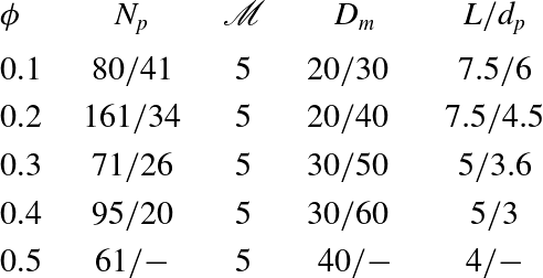
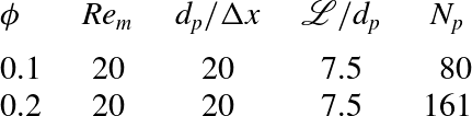
where the square brackets denote the nearest integer. The various numerical parameters used in the simulations are reported in table 1.
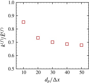
The convergence of
 $k^{(f)}/\bar{E}^{(f)}$
with respect to the grid resolution
 $D_{m}$
for a solid volume fraction of 0.3 and mean slip Reynolds number of 20 is shown in figure 4. The grid resolutions used in the PUReIBM simulations (see table 1) have been chosen such that they yield numerically converged solutions. The values provided in table 1 guarantee that the particle mean drag force is also converged (Tenneti et al.
Reference Tenneti, Garg and Subramaniam2011). The level of
 $k^{(f)}/\bar{E}^{(f)}$
for a specific random particle assembly clearly shows numerical convergence as the grid resolution is increased.
Convergence characteristics of
 $k^{(f)}/\bar{E}^{(f)}$
with grid resolution
 $d_{p}/{\rm\Delta}x$
for flow past a random particle configuration at
 ${\it\phi}=0.3$
and
 $\mathit{Re}_{m}=20$
. The random configuration is the same for all grid resolutions.

Numerical parameters (number of particles
 $N_{p}$
, number of MIS
 $\mathscr{M}$
, particle diameter in grid units
 $D_{m}$
and the ratio of the length of the box to the particle diameter
 $L/d_{p}$
) used for random arrays in PUReIBM simulations. Different numerical parameters are used for
 $\mathit{Re}_{m}\leqslant 100$
and
 $\mathit{Re}_{m}>100$
. These are separated by a ‘/’. Numbers before the ‘/’ correspond to
 $\mathit{Re}_{m}\leqslant 100$
while numbers after the ‘/’ correspond to
 $\mathit{Re}_{m}>100$
. At volume fraction 0.5 PUReIBM simulations are performed only up to a Reynolds number of 100.

The convergence of the ensemble-averaged
 $k^{(f)}$
with 65 realizations for the case
 ${\it\phi}=0.4$
and
 $Re_{m}=100$
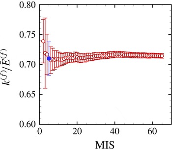
is shown in figure 5. This figure indicates that the ensemble-averaged mean obtained with 65 realizations lies within the 95 % confidence intervals obtained with five realizations (highlighted as the filled symbol in figure 5). Moreover, the 95 % confidence intervals for five realizations represent less than 5 % deviation from the evaluated average. Therefore, five independent realizations were simulated for all the cases shown in table 1.
Convergence characteristics of
 $k^{(f)}/\bar{E}^{(f)}$
with number of realizations for flow past random arrays of spheres at
 ${\it\phi}=0.4$
and
 $\mathit{Re}_{m}=100$
. The error bars denote 95 % confidence intervals in the estimation of the average
 $k^{(f)}$
. The filled symbol represents the level of
 $k^{(f)}$
corresponding to five realizations.

Besides convergence with the grid resolution and number of realizations, it is also important to check whether the box size is adequate or not. The box size is deemed adequate if the two-point correlation functions in the fluid phase decay to zero within the box length. To check this, the two-point velocity correlation function for the streamwise component of the velocities has been computed for the highest Reynolds number simulated. The fluid-phase velocity autocorrelation
 ${\it\rho}_{u_{\Vert }}\left(r\right)$
is defined as
 $$\begin{eqnarray}{\it\rho}_{u_{\Vert }}\left(r\right)=\frac{\left\langle I_{f}\left(\boldsymbol{x}\right)u_{\Vert }^{\prime \prime (f)}\left(\boldsymbol{x}\right)I_{f}\left(\boldsymbol{x}+\boldsymbol{r}\right)u_{\Vert }^{\prime \prime (f)}\left(\boldsymbol{x}+\boldsymbol{r}\right)\right\rangle }{\left\langle I_{f}u_{\Vert }^{\prime \prime (f)}u_{\Vert }^{\prime \prime (f)}\right\rangle },\end{eqnarray}$$
where
 $r=|\boldsymbol{r}|$
and
 $u_{\Vert }^{\prime \prime (f)}$
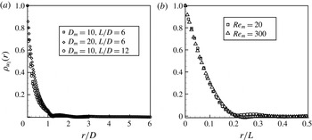
is the streamwise component of the gas-phase velocity fluctuation. Figure 6(a) shows the convergence of the fluid-phase velocity autocorrelation function with the grid resolution as well as the box size for a random configuration of particles at a solid volume fraction of 0.2 and a Reynolds number of 20. The autocorrelation function has also been computed for the highest Reynolds number that we simulated and is shown in figure 6(b). These results clearly indicate that the numerical parameters used in our simulation are adequate to obtain numerically converged results for
 $k^{(f)}$
. We now present the results obtained from PUReIBM simulations of flow past monodisperse fixed particle assemblies.
(a) Convergence of the fluid-phase velocity autocorrelation function with the grid resolution as well as the box size for a random configuration of particles at a solid volume fraction of 0.2 and a Reynolds number of 20. (b) Decay of the fluid velocity autocorrelation function obtained from PUReIBM simulation of steady flow past a random configuration of spheres at a solid volume fraction of 0.2 and mean slip Reynolds numbers of 20 (squares) and 300 (triangles). In these simulations
 $L/d_{p}$
ratios of 6 and 4.5 are used for Reynolds numbers of 20 and 300 respectively.

6. Gas-phase velocity fluctuations in steady flow past fixed particle assemblies
While the evolution of the gas-phase velocity fluctuations due to particles has been studied for zero mean slip (Cate et al. Reference Cate, Derksen, Portela and van den Akker2004; Zhang & Prosperetti Reference Zhang and Prosperetti2005; Lucci, Ferrante & Elghobashi Reference Lucci, Ferrante and Elghobashi2010), the mean slip velocity between the phases is non-zero in fluidized beds. Xu & Subramaniam (Reference Xu and Subramaniam2010) studied the interaction of a turbulent upstream flow with a fixed particle assembly in an attempt to reproduce the experimental findings of Moran & Glicksman (Reference Moran and Glicksman2003). In their study the upstream flow is initialized with isotropic turbulence and drawn through a uniform configuration of fixed particles by imposing a mean constant pressure gradient. This flow is inhomogeneous in the mean flow direction, but gas-phase velocity fluctuations reach a constant value within three particle diameters of entering the bed. The significant result of this study is the enhancement of turbulence as it interacts with solid spheres of the fixed bed.
In the current study we simulate initially turbulent flow in fixed particle assemblies to quantify the relative magnitude of gas-phase velocity fluctuations arising from turbulent and pseudo-turbulent sources. It should be noted that the initial isotropic turbulence is not sustained by artificial forcing and decays in time. The particle configurations correspond exactly to the uniformly distributed particle configurations of Xu & Subramaniam (Reference Xu and Subramaniam2010). These configurations are uniform distributions of non-overlapping spheres generated using the Matérn hard-core point process (Stoyan, Kendall & Mecke Reference Stoyan, Kendall and Mecke1995). This process is essentially a Poisson point process for particle centres from which overlapping spheres have been removed using an approach called dependent thinning. To address the level of turbulent and pseudo-turbulent gas-phase velocity fluctuations we consider three types of simulations:
-
(a) Case I initialized with a non-turbulent uniform laminar flow.
-
(b) Case II initialized with an isotropic turbulent flow.
-
(c) Case III initialized with the steady solution of Case I to which the initial isotropic turbulence of Case II is added.
The simulations start by imposing a mean pressure gradient along the mean flow such that the Reynolds number reaches the desired value. The mean slip Reynolds number is 50 with four realizations for all cases. Detailed information on the flow parameters is provided in table 2.
Numerical and physical parameters of the turbulent/pseudo-turbulent simulations: solid-phase volume fraction
 ${\it\phi}$
, mean slip Reynolds number
 $Re_{m}$
, Taylor microscale turbulent Reynolds number
 $Re_{{\it\lambda}}$
, particle diameter to dissipative length scale ratio
 $d_{p}/{\it\eta}$
, particle diameter in grid units
 $d_{p}/{\rm\Delta}x$
, computational box length to particle diameter ratio
 $\mathscr{L}/d_{p}$
and number of particles
 $N_{p}$
.

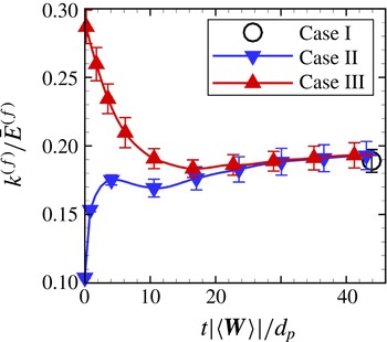
Case I is simply PR-DNS of a uniformly distributed fixed particle assembly initialized with non-turbulent uniform laminar flow, and the corresponding steady value of
 $k^{(f)}$
is shown as circles in figure 7. The initial isotropic turbulence in Case II is generated by the method described by Rogallo (Reference Rogallo1981) for a Taylor microscale turbulent Reynolds number
 $Re_{{\it\lambda}}$
of 12 with the energy spectrum function given by Pope (Reference Pope2000). The corresponding Kolmogorov length scale is selected such that the ratio
 $d_{p}/{\it\eta}$
is 5. Although the
 $Re_{{\it\lambda}}$
obtained from scaling analysis in experimental studies could be relatively high (the turbulent Reynolds number
 $Re_{{\it\lambda}}$
is approximately 50 in the work of Moran & Glicksman Reference Moran and Glicksman2003), we are naturally limited by computational resources to lower initial
 $Re_{{\it\lambda}}$
because particle-resolved simulations for
 $d_{p}/{\it\eta}>1$
impose additional computational overhead. This is because the mean slip velocity generates flow structures that need to be resolved in PR-DNS (for estimates of computational cost, see for instance Xu & Subramaniam Reference Xu and Subramaniam2010).
Evolution of
 $k^{(f)}$
normalized by the mean flow energy
 $\bar{E}^{(f)}$
versus time normalized by the characteristic flow time scale
 $d_{p}/|\langle \boldsymbol{W}\rangle |$
. The symbols ▿ correspond to the simulation initialized with an isotropic turbulence. The symbols ▵ represent simulation of the perturbed velocity field. The symbol ○ shows the steady value of the gas-phase pseudo-turbulence.

Figure 7 also indicates that for Case II, the level of
 $k^{(f)}$
starts from the specified initial isotropic turbulence level and increases to the steady-state pseudo-turbulent value. The data reveal that the velocity fluctuations arising from the presence of particles in the flow with non-zero mean slip velocity are much higher than the turbulent velocity fluctuations for
 $Re_{{\it\lambda}}=12$
, and the principal contribution to the gas-phase velocity fluctuations is the pseudo-turbulent part.
Since in this study the configurations and simulation parameters are the same as those chosen by Xu & Subramaniam (Reference Xu and Subramaniam2010), we can compare the
 $k^{(f)}$
values between these homogeneous PUReIBM simulations and the inflow/outflow simulations of Xu & Subramaniam (Reference Xu and Subramaniam2010). In their study, the flow is inhomogeneous along the flow direction and
 $k^{(f)}$
is reported along the mean flow direction. The level of
 $k^{(f)}$
increases from the beginning of the bed; it represents a 100 % increase from the entrance of the particle bed and reaches a constant value after an entrance length of
 $3d_{p}$
. Our homogeneous simulation results are similar for Case II, where the normalized
 $k^{(f)}$
starts from an initial value of 0.1 and reaches approximately twice its initial value (0.19) at steady state. This indicates that the enhancement observed by Xu & Subramaniam (Reference Xu and Subramaniam2010) is mainly due to the pseudo-turbulent velocity fluctuations, an observation corroborated by experiment (Moran & Glicksman Reference Moran and Glicksman2003).
Case III is basically used to examine the relaxation of turbulence in particle-laden flows. The evolution of
 $k^{(f)}$
for Case III in figure 7 shows that the excess amount of
 $k^{(f)}$
decays and the pseudo-turbulent steady-state level of
 $k^{(f)}$
is recovered. These results, showing both attenuation and enhancement of turbulence depending on the initial level of velocity fluctuations, indicate that for this choice of
 ${\it\phi}$
and
 $Re_{m}$
, initial turbulent motions in the gas phase do not influence the steady value of
 $k^{(f)}$
, which corresponds to the pseudo-turbulent fluctuations arising from the interaction of particles with the mean flow. Since the mechanisms for generation and dissipation of these contributions to
 $k^{(f)}$
are different, this provides useful information for the development of predictive multiphase turbulence models in this regime of gas–solid flow. Therefore, in the following sections we focus on quantifying the level of pseudo-turbulence and the corresponding dissipation rate over a wide range of flow parameters.
Variation of
 $k^{(f)}$
normalized by
 $\bar{E}^{(f)}=(1/2)\langle \boldsymbol{u}^{(f)}\rangle \boldsymbol{\cdot }\langle \boldsymbol{u}^{(f)}\rangle$
with
 $\mathit{Re}_{m}$
and
 ${\it\phi}$
. (a) The behaviour of
 $k^{(f)}/\bar{E}^{(f)}$
with
 ${\it\phi}$
for different mean slip Reynolds numbers.(b) The behaviour of
 $k^{(f)}/\bar{E}^{(f)}$
with
 $\mathit{Re}_{m}$
for different solid volume fractions.

7. Quantification of PTKE from PR-DNS
We performed PUReIBM DNS of flow past fixed assemblies of monodisperse spheres over a wide range of solid volume fractions (
 $0.1\leqslant {\it\phi}\leqslant 0.5$
) and mean slip Reynolds numbers (
 $0.01\leqslant \mathit{Re}_{m}\leqslant 300$
) to quantify the level of PTKE in terms of
 ${\it\phi}$
and
 $\mathit{Re}_{m}$
. All simulations start with the initial condition of uniform fluid velocity. We have shown in the previous section that initializing the simulations with a homogeneous isotropic turbulent velocity field does not affect the steady value of
 $k^{(f)}$
attained by the system. Therefore, the steady-state value of
 $k^{(f)}$
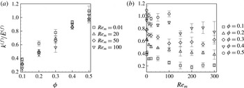
obtained in a fixed particle assembly depends only on the solid volume fraction and the mean slip Reynolds number. Figure 8(a) shows the variation of
 $k^{(f)}/\bar{E}^{(f)}$
with the solid volume fraction for different mean slip Reynolds numbers, while figure 8(b) shows the variation of
 $k^{(f)}/\bar{E}^{(f)}$
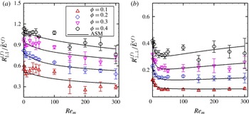
with mean slip Reynolds number for different solid volume fractions. As is evident from figure 8(a), the PTKE normalized by the mean energy in the gas phase increases dramatically with the volume fraction. As shown in figure 8(b), at a given volume fraction
 $k^{(f)}/\bar{E}^{(f)}$
decreases rapidly with increasing mean slip Reynolds number up to
 $\mathit{Re}_{m}=50$
, and beyond
 $\mathit{Re}_{m}=50$
it has a weak power law dependence on
 $\mathit{Re}_{m}$
. This behaviour is a result of the normalization of
 $k^{(f)}$
by
 $\bar{E}^{(f)}$
. It implies that the variance of gas velocity increases approximately as the square of the mean slip Reynolds number. Since the total kinetic energy of the gas increases with increasing mean flow Reynolds number, we expect the strength of gas-phase velocity fluctuations to also increase. Using the data obtained from PUReIBM DNS we found that the following function fits the data for PTKE with an average deviation of 5 %:
 $$\begin{eqnarray}\displaystyle & & \displaystyle \frac{k^{(f)}}{\bar{E}^{(f)}}\left({\it\phi},\mathit{Re}_{m}\right)=2{\it\phi}+2.5{\it\phi}\left(1-{\it\phi}\right)^{3}\exp \!\left(-{\it\phi}{\mathit{Re}_{m}}^{1/2}\right)\!,\nonumber\\ \displaystyle & & \displaystyle \quad 0.1\leqslant {\it\phi}\leqslant 0.5,0.01\leqslant \mathit{Re}_{m}\leqslant 300.\end{eqnarray}$$
As shown in (7.1), the correlation is proposed from simulations in the range
 $0.1\leqslant {\it\phi}\leqslant 0.5$
and
 $0.01\leqslant \mathit{Re}_{m}\leqslant 300$
. The value of
 $k^{(f)}/\bar{E}^{(f)}$
from (7.1) tends to appropriate values in the limit of infinite dilution and creeping flow. In the limiting case of infinite dilution, i.e.
 ${\it\phi}\rightarrow 0$
, the value of
 $k^{(f)}/\bar{E}^{(f)}$
is zero. This limiting value is consistent with the fact that in the absence of particles the flow field is uniform. In the Stokes flow regime (
 $\mathit{Re}_{m}\rightarrow 0$
) the value of
 $k^{(f)}/\bar{E}^{(f)}$
reaches an asymptote and depends only on the solid volume fraction. This behaviour is consistent with the fact that the mean drag (which is shown to be the source of
 $k^{(f)}$
in the next section) acting on the particles is linear in the Stokes flow regime and thus the normalized quantity
 $k^{(f)}/\bar{E}^{(f)}$
is independent of the Reynolds number.
Although our study is for homogeneous gas–solid suspensions, the dependence of
 $k^{(f)}$
on the solid volume fraction and mean slip Reynolds number has implications for transport of the gas-phase Reynolds stress in inhomogeneous flows also. The strong dependence of
 $k^{(f)}$
on
 ${\it\phi}$
suggests that the transport of
 $k^{(f)}$
could be significant in statistically inhomogeneous flows with spatial variation of
 ${\it\phi}$
. The quantification of the dissipation of PTKE in the gas phase is discussed in the following section.
8. Reynolds stress tensor of pseudo-turbulent gas-phase velocity fluctuations
The gas-phase Reynolds stress is defined as
 $$\begin{eqnarray}R_{ij}^{(f)}=\frac{\left\langle I_{f}u_{i}^{\prime \prime (f)}u_{j}^{\prime \prime (f)}\right\rangle }{\left\langle I_{f}\right\rangle },\end{eqnarray}$$
and its trace represents the level of gas-phase velocity fluctuations
 $k^{(f)}$
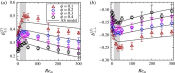
. The presence of particles introduces anisotropy in the gas-phase Reynolds stress that in turn modifies the structure of the carrier phase by extending them along the mean flow (Uhlmann Reference Uhlmann2008; Xu & Subramaniam Reference Xu and Subramaniam2010). The gas-phase anisotropy tensor
 $$\begin{eqnarray}b_{ij}^{(f)}=\frac{R_{ij}^{(f)}}{2k^{(f)}}-\frac{1}{3}{\it\delta}_{ij},\end{eqnarray}$$
is computed along the streamwise (parallel to mean slip) and spanwise (perpendicular to mean slip) directions and presented in figure 9(a,b) respectively. The results indicate that the cross-correlation of velocity fluctuations
 $b_{\Vert ,\bot }^{(f)}$
is negligible (not shown here), and the normal component in the parallel direction
 $b_{\Vert ,\Vert }^{(f)}$
is dominant compared with the component in the perpendicular direction
 $b_{\bot ,\bot }^{(f)}$
. Hence, the state of pseudo-turbulent gas-phase velocity fluctuations is axisymmetric (Pope Reference Pope2000).
Figure 9 indicates that the level of anisotropy increases with
 $Re_{m}$
from Stokes flow to moderate Reynolds numbers (ranging from 10 to 40) and then smoothly decreases. We hypothesize that this variation in anisotropy is related to the ratio of the length scale associated with gas-phase velocity fluctuations to the local average interparticle spacing. These length scales are quantified using our simulations.
Deviatoric tensor components are shown for different
 ${\it\phi}$
and
 $Re_{m}$
obtained from fixed-bed simulations. The symbols show our PR-DNS data while the solid lines represent the model proposed in (8.6) and (8.7). The shaded region indicates where the maximum anisotropy occurs. (a) Parallel to the mean slip. (b) Perpendicular to the mean slip.

Increase of Reynolds number from low-
 $Re_{m}$
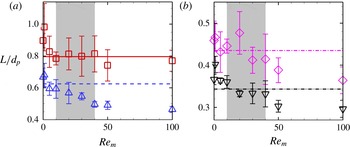
flow initiates the separation of boundary layer around particles and a standing eddy forms behind spheres with a characteristic length (Pruppacher, Le Clair & Hamielec Reference Pruppacher, Le Clair and Hamielec1970), which is a source of anisotropy in gas-phase Reynolds stress (Mohd-Yusof Reference Mohd-Yusof1996; Uhlmann Reference Uhlmann2008). However, definition of an appropriate length scale for gas-phase velocity fluctuations in a random particle assembly is not straightforward since the wakes are affected by the presence of neighbouring particles. We use the Eulerian two-point correlation of gas-phase velocity fluctuations to define a characteristic length for gas-phase velocity fluctuations
 $L_{\Vert ,\Vert }$
as follows:
 $$\begin{eqnarray}L_{\Vert ,\Vert }=\frac{1}{R_{\Vert ,\Vert }^{(f)}(0)}\int _{0}^{\infty }R_{\Vert ,\Vert }^{(f)}(r)\text{d}r,\end{eqnarray}$$
where
 $R_{\Vert ,\Vert }^{(f)}(r)$
is
 $$\begin{eqnarray}R_{\Vert ,\Vert }^{(f)}(r)=\frac{1}{V^{(f)}}\int _{\mathscr{V}^{(f)}}u_{\Vert }^{\prime \prime (f)}(\boldsymbol{x})u_{\Vert }^{\prime \prime (f)}(\boldsymbol{x}+\boldsymbol{r})\text{d}V,\end{eqnarray}$$
the two-point correlation in the parallel direction. This length scale of gas-phase velocity fluctuations, shown in figure 10, decreases with
 $Re_{m}$
due to the fact that the flow structures become finer and less correlated to other surrounding structures. In addition, increase of the solid volume fraction makes the gas-phase velocity fluctuations become less spatially correlated due to the influence of nearby particles, and hence the length scale decreases.
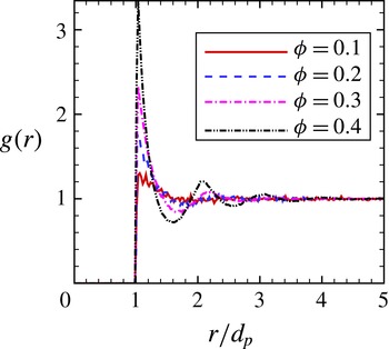
We use the radial distribution function
 $g(r)$
to define a characteristic local interparticle spacing within a neighbourhood of a test particle. It should be noted that other studies used a similar approach to compute the nearest neighbour distance for point particles (Hertz Reference Hertz1909) and finite size particles (Torquato, Lu & Rubinstein Reference Torquato, Lu and Rubinstein1990) in random particle arrangements. The radial distribution function is shown in figure 11 for different volume fractions. The radial distribution is the probability of finding a particle at separation
 $r$
given that there is a particle at the coordinate origin. By assuming a spherical shell of volume
 $4{\rm\pi}r^{2}\;{\it\delta}r$
at separation
 $r$
, the number of particles in the shell is
 $2{\rm\pi}N_{p}\;n\;g(r)r^{2}\;{\it\delta}r$
. Thus, we compute the local interparticle spacing of the suspension using the expression
 $$\begin{eqnarray}\frac{L_{int}}{d_{p}}=\frac{1}{d_{p}}\;\frac{\displaystyle \int _{d_{p}}^{R}g(r)\;r^{2}\;l\;f(l)\text{d}r}{\displaystyle \int _{d_{p}}^{R}g(r)\;r^{2}\;f(l)\text{d}r},\end{eqnarray}$$
which is a weighted average of distances among particles in a spherical shell between the minimum separation
 $d_{p}$
and
 $R$
. In (8.5),
 $l$
is the surface to surface distance, defined as
 $r-d_{p}$
, and
 $f(l)$
is a weight function. We choose
 $R$
as the second peak of
 $g(r)$
, which includes all particles in the local neighbourhood of the test particle. The weight function is assumed to have the form
 $1/l^{p}$
with
 $p\geqslant 0$
. It should be noted that the choice of
 $p=0$
causes
 $L_{int}$
to be equally weighted by neighbouring particles, while choosing higher values for
 $p$
preferentially weights the most proximate particles. We select
 $p=1$
, a value that takes into account the importance of all particles in the region between
 $d_{p}$
and
 $R$
in a manner where proximate particles contribute more to the local interparticle spacing.
The symbols show the length scale of gas-phase velocity fluctuations
 $L_{\Vert ,\Vert }$
, while the straight lines show the corresponding local interparticle spacing
 $L_{int}$
. The shaded region shows where the maximum anisotropy occurs. In (a)
 ${\it\phi}=0.1$
(▫),
 ${\it\phi}=0.2$
(▵). In (b)
 ${\it\phi}=0.3$
(♢),
 ${\it\phi}=0.4$
(▿).

Radial distribution function estimated from 100 realizations for different
 ${\it\phi}$
.

The results indicate that the local interparticle spacings (shown as straight lines in figure 10) intersect the length scales of gas-phase velocity fluctuations at the Reynolds numbers where the anisotropy starts to decrease (figure 9). At low Reynolds numbers, flow structures formed behind particles elongate with
 $Re_{m}$
, which gives rise to the increase of anisotropy. At moderate Reynolds numbers (
 $10\leqslant Re_{m}\leqslant 40$
), the wakes become as large as the gaps among particles and are broken up due to interaction with neighbouring spheres. Thus, the magnitude of anisotropy is determined by the ratio of the gas-phase velocity fluctuation length scale to the local interparticle spacing. The breakup of elongated structures redistributes the energy of the fluctuating velocities among Reynolds stress components and decreases the anisotropy.
It is also observed that increase of the solid volume fraction causes an attenuation in the level of anisotropy. Increase of the solid volume fraction lessens the local interparticle gaps and does not allow the formation of distinct wake structures (Reddy et al.
Reference Reddy, Sathe, Joshi, Nandakumar and Evans2013), leading to a decrease in anisotropy. This is confirmed in figure 10, since the length scale of gas-phase velocity fluctuations decreases with the volume fraction. Breault, Guenther & Shadle (Reference Breault, Guenther and Shadle2008) also reported that the axial solid dispersion coefficient of particles in a particle-laden flow decreases with the volume fraction, which is interpreted as decrease of
 $R_{\Vert ,\Vert }$
while
 $R_{\bot ,\bot }$
increases, and our data are in agreement with this trend observed in experiments.
Using the gas-phase anisotropy data obtained from our PR-DNS and considering the aforementioned physics explaining the behaviour of gas-phase anisotropy, we found that the following function fits the data for the gas-phase anisotropy:
 $$\begin{eqnarray}\displaystyle & \displaystyle b_{\Vert ,\Vert }^{(f)}({\it\phi},Re_{m})=\frac{a}{1+b\;\exp (-c\;Re_{m})}\;\exp \!\left(\frac{-d\;{\it\phi}}{1+e\;\exp (-f\;Re_{m})}\right), & \displaystyle\end{eqnarray}$$
 $$\begin{eqnarray}\displaystyle & \displaystyle b_{\bot ,\bot }^{(f)}({\it\phi},Re_{m})=-\frac{b_{\Vert ,\Vert }({\it\phi},Re_{m})}{2}, & \displaystyle\end{eqnarray}$$
 $a=0.523$
,
 $b=0.305$
,
 $c=0.114$
,
 $d=3.511$
,
 $e=1.801$
and
 $f=0.005$
. This model asymptotically reaches a constant value for a fixed
 ${\it\phi}$
(not shown here) that guarantees that the normal components of the gas-phase anisotropy remain non-zero. This model and the model proposed for
 $k^{(f)}$
in (7.1) can be used together to propose an ASM for the pseudo-turbulent gas-phase Reynolds stress in the form of
 $$\begin{eqnarray}\frac{R_{ij}^{(f)}}{\bar{E}^{(f)}}=2\;\left(b_{ij}^{(f)}+\frac{1}{3}{\it\delta}_{ij}\right)\;\frac{k(f)}{\bar{E}^{(f)}}\;.\end{eqnarray}$$
Comparison of this ASM with PR-DNS data as shown in figure 12 indicates that the model appropriately predicts the non-zero components of the pseudo-turbulent gas-phase Reynolds stress. A noteworthy feature of this model is that in the limit of
 ${\it\phi}\rightarrow 0$
, the gas-phase Reynolds stress becomes zero and the system reduces to a laminar single-phase flow without any pseudo-turbulent velocity fluctuations.
9. Gas-phase velocity fluctuations in freely evolving suspensions
Although fixed beds are good approximations to particle-laden flows at high particle Stokes number, in reality each sphere moves with an acceleration arising from hydrodynamic and collisional forces. Simulation of freely evolving suspensions enables us to study the effect of physical parameters such as the solid-to-gas density ratio and coefficient of restitution, in addition to the solid volume fraction and Reynolds number that are used to characterize fixed-bed simulations. It should be noted that these freely evolving simulations complement the study of Yin et al. (Reference Yin, Zenk, Mitrano and Hrenya2013) by exploring the
 $Re_{m}$
axis of the parameter space, whereas their work explores the granular temperature dependence for zero
 $Re_{m}$
.
The gas-phase Reynolds stress tensor is shown for different
 ${\it\phi}$
and
 $Re_{m}$
. The symbols show our PR-DNS data while the solid lines represent the model proposed in (8.8). (a) Parallel to the mean slip. (b) Perpendicular to the mean slip.

In our freely evolving suspension study, a mean pressure is imposed along the mean flow direction such that a desired mean slip Reynolds number is achieved. All our simulations are performed at a mean slip Reynolds number of
 $Re_{m}=20$
with five independent realizations for each case. Detailed information on particle configurations is provided in table 3. The influence of the solid volume fraction is studied by simulating two volume fractions
 ${\it\phi}=0.1$
and 0.2. The simulations are initialized with a uniform mean flow for the gas phase and zero granular temperature for the solid phase, and are carried out until a steady value of
 $k^{(f)}$
is attained.
The numerical and physical parameters of the freely evolving suspensions.

9.1. Effect of particle-to-fluid density ratio
To investigate the effect of the particle-to-gas density ratio we simulated two density ratio values of
 ${\it\rho}^{(p)}/{\it\rho}^{(f)}=100$
and 1000. These density ratios are associated with particle Stokes numbers (the ratio of the particle response time
 ${\it\tau}_{p}={\it\rho}^{(p)}d_{p}^{2}/(18{\it\rho}^{(f)}{\it\nu}^{(f)})$
to the fluid characteristic time scale
 ${\it\tau}_{f}=d_{p}/|\langle \boldsymbol{W}\rangle |$
) in the range of 123–1390 for the cases considered in this study. The comparison of
 $k^{(f)}$
for the two density ratios with elastic particles indicates that the level of gas-phase velocity fluctuations is not significantly influenced by the particle density, as shown in figure 13. In this figure,
 $k^{(f)}$
increases rapidly and then attains a relatively constant value. The evolution of
 $k^{(f)}$
is also compared with fixed-bed results at the same Reynolds number and solid volume fractions, represented by dashed lines in the figure. The difference of
 $k^{(f)}$
in a freely evolving suspension from its value in the corresponding fixed bed is less than 10 %. This establishes the validity of using fixed-bed simulations as an approximation to high-Stokes-number suspensions undergoing elastic collisions, as employed in earlier studies (Tenneti et al.
Reference Tenneti, Garg, Hrenya, Fox and Subramaniam2010; Xu & Subramaniam Reference Xu and Subramaniam2010).
Evolution of
 $k^{(f)}$
normalized by mean flow energy for elastic particles with different
 ${\it\phi}$
and
 ${\it\rho}^{(p)}/{\it\rho}^{(f)}$
. Fixed-bed values at
 ${\it\phi}=0.1$
and 0.2 are shown for comparison.

Traditionally it has been assumed that the energy in the gas-phase velocity fluctuations is at best a small fraction of the energy in the particle velocity fluctuations and the energy associated with the mean flow. Therefore, it is of interest to quantify the relative magnitude of the kinetic energy in the fluctuating velocities of the gas and solid phases, as shown in figure 14 for density ratios of
 ${\it\rho}^{(p)}/{\it\rho}^{(f)}=100$
and 1000. These density-weighted energies are computed as
 $\tilde{e}^{(f)}={\it\rho}^{(f)}(1-{\it\phi})k^{(f)}$
in the gas phase and
 $\tilde{e}^{(p)}={\it\rho}^{(p)}{\it\phi}\;k^{(p)}$
in the solid phase, normalized by the kinetic energy in the mean slip
 $\tilde{E}^{(f)}={\it\rho}^{(f)}\bar{E}^{(f)}$
. The energy in the solid-phase fluctuating velocities
 $k^{(p)}$
is defined as
 $\langle \boldsymbol{u}^{\prime \prime (p)}\boldsymbol{\cdot }\boldsymbol{u}^{\prime \prime (p)}\rangle /2$
, where
 $\boldsymbol{u}^{\prime \prime (p)}=\boldsymbol{u}^{(p)}-\langle \boldsymbol{u}^{(p)}\rangle$
is the solid-phase velocity fluctuation. Figure 14 shows that the amount of energy in the gas-phase velocity fluctuations
 $\tilde{e}^{(f)}$
is comparable to that in the solid phase, and both are significant compared with the energy of the mean slip. In other words, the kinetic energy of the gas phase is as important as the kinetic energy of the solid phase, and cannot be neglected in modelling of gas–solid flows.
Comparison of the density-weighted kinetic energy in gas and solid velocity fluctuations normalized by the fluid energy corresponding to the mean slip velocity, for (a)
 ${\it\rho}^{(p)}/{\it\rho}^{(f)}=100$
and (b)
 ${\it\rho}^{(p)}/{\it\rho}^{(f)}=1000$
.

9.2. Effect of coefficient of restitution in particle collisions
In freely evolving suspensions with inelastic particle collisions, the energy of the system is dissipated by collisional dissipation among particles as well as viscous dissipation of the carrier flow. We compare the effect of the coefficient of restitution (COR) on
 $k^{(f)}$
in figure 15 for three values of COR, 1.0, 0.9 and 0.7. Figure 15 shows that
 $k^{(f)}$
is not very sensitive to COR and the differences are not statistically significant, especially for the lower volume fraction. In addition, as figure 15(a,b) shows, the density ratio has a negligible effect on the level of
 $k^{(f)}$
for inelastic particles. As in the case of elastic particles, the level of
 $k^{(f)}$
is in good agreement with that for a fixed bed (refer to figure 13), with a maximum difference of 15 % for the higher volume fraction. The weak dependence of
 $k^{(f)}$
on the inelasticity of particles further strengthens the validity of using fixed beds as an approximation to high-Stokes-number suspensions.
Comparison of
 $k^{(f)}$
normalized by the mean flow energy for freely evolving suspensions undergoing elastic collisions (
 $\text{COR}=1$
) with those undergoing inelastic collisions (
 $\text{COR}<1$
), for (a)
 ${\it\rho}^{(p)}/{\it\rho}^{(f)}=100$
and (b)
 ${\it\rho}^{(p)}/{\it\rho}^{(f)}=1000$
.

The independence of
 $k^{(f)}$
with respect to COR suggests that these suspensions belong to a regime that is dominated by viscous dissipation, as opposed to the collisionally dissipative regime (Sangani et al.
Reference Sangani, Mo, Tsao and Koch1996). To precisely characterize the regime of the gas–solid flows examined in this study, we quantify the ratio of the time taken by gas-phase forces to affect particle motion
 $t_{\mathit{hydro}}$
to the average time between collisions
 $t_{\mathit{coll}}$
(Wylie, Koch & Ladd Reference Wylie, Koch and Ladd2003). The time scale over which the particle responds to hydrodynamic forces is defined as
 $$\begin{eqnarray}t_{\mathit{hydro}}=\frac{\sqrt{3T}}{{\it\sigma}_{A}},\end{eqnarray}$$
where
 $T=\langle \boldsymbol{u}^{\prime \prime (p)}\boldsymbol{\cdot }\boldsymbol{u}^{\prime \prime (p)}\rangle /3$
is the granular temperature and
 ${\it\sigma}_{A}$
characterizes the standard deviation in particle accelerations. In order to calculate the mean collisional time scale from our PR-DNS data, we first compute
 $\bar{N}_{\mathit{coll}}$
, the mean number of collisions per particle in the domain, and then divide the corresponding sampling time
 $\bar{t}$
by this mean value, i.e.
 $t_{\mathit{coll}}=\bar{t}/\bar{N}_{\mathit{coll}}$
. Wylie et al. (Reference Wylie, Koch and Ladd2003) reported that the flow is collision-dominant if the hydrodynamic-to-collisional time scale ratio is much larger than 1, i.e.
 $t_{\mathit{hydro}}/t_{\mathit{coll}}\gg 1\sim O(10)$
. Figure 16 indicates that this ratio is less than unity for the cases simulated in this study. This confirms that the time required for the gas-phase stresses to influence particle motion is less than the mean time between the collisions (
 $t_{\mathit{hydro}}<t_{\mathit{coll}}$
). In other words, these gas–particle systems are dominated by viscous forces, and therefore the energy loss due to collisional dissipation does not significantly affect the evolution of
 $k^{(f)}$
. Consequently, the energy of gas-phase fluctuating velocities evolves in a manner similar to fixed particle assemblies.
Hydrodynamic time scale to collisional time scale ratio.

9.3. Energy transfer from mean flow to velocity fluctuations
The principle of conservation of interphase TKE transfer proposed by Xu & Subramaniam (Reference Xu and Subramaniam2007) states that
 ${\it\Pi}^{(m)}$
, the rate of work done by the mean pressure gradient in moving the flow at the prescribed mean slip velocity, is partitioned into sources of interphase TKE transfer in the fluid phase (
 ${\it\Pi}^{(f)}$
) and the solid phase (
 ${\it\Pi}^{(p)}$
), such that
 $$\begin{eqnarray}{\it\Pi}^{(m)}=\left\langle \boldsymbol{W}\right\rangle \boldsymbol{\cdot }\left\langle \boldsymbol{S}_{M}^{(f)}\right\rangle ={\it\Pi}^{(f)}+{\it\Pi}^{(p)},\end{eqnarray}$$
where
 $\langle S_{Mi}^{(f)}\rangle =\langle {\it\tau}_{ji}n_{j}^{(f)}{\it\delta}(\boldsymbol{x}-\boldsymbol{x}^{(\boldsymbol{I})})\rangle$
is the average momentum transfer between the gas and the solid phases that balances the mean pressure gradient at steady state. The source terms
 ${\it\Pi}^{(f)}$
and
 ${\it\Pi}^{(p)}$
appear in the evolution equations for
 $k^{(f)}$
and
 $k^{(p)}$
respectively, and these are given below. While in fixed beds
 ${\it\Pi}^{(p)}=0$
, the solid-phase interphase TKE transfer is non-zero in freely evolving suspensions.
The evolution of
 $k^{(f)}$
for a homogeneous suspension is given by (Xu & Subramaniam Reference Xu and Subramaniam2007; Pai & Subramaniam Reference Pai and Subramaniam2009)
 $$\begin{eqnarray}\underbrace{{\it\rho}^{(f)}(1-{\it\phi})\frac{\text{d}k^{(f)}}{\text{d}t}}_{\text{unsteady}~\text{term}}=\underbrace{\left\langle u_{i}^{\prime \prime (f)}{\it\tau}_{ji}n_{j}^{(f)}{\it\delta}\left(\boldsymbol{x}-\boldsymbol{x}^{(\boldsymbol{I})}\right)\right\rangle }_{{\it\Pi}^{(f)}}+\left\langle u_{i}^{\prime \prime (f)}\frac{\partial (I_{f}{\it\tau}_{ji})}{\partial x_{j}}\right\rangle ,\end{eqnarray}$$
where
 $\boldsymbol{n}^{(f)}$
is the unit normal vector pointing outward from the gas phase into the solid phase. The gas-phase interphase TKE transfer
 ${\it\Pi}^{(f)}$
in (9.3) arises from the fluctuating velocity–stress tensor covariance only at the gas–solid interface, while it is zero in the bulk flow due to the Dirac delta function. The second term on the right-hand side of (9.3) is the covariance of the fluctuating fluid velocity field and the gradient of the stress tensor in the fluid phase. For statistically homogeneous flows this term simplifies (cf. appendix A) to
 $-2{\it\mu}^{(f)}\langle I_{f}s_{ij}s_{ij}\rangle$
, where
 ${\it\varepsilon}^{(f)}=2{\it\mu}^{(f)}\langle I_{f}s_{ij}s_{ij}\rangle$
can be identified as the dissipation that is strictly non-negative. Here,
 $s_{ij}=(\partial u_{i}^{\prime \prime (f)}/\partial x_{j}+\partial u_{j}^{\prime \prime (f)}/\partial x_{i})/2$
is the strain rate of the fluctuating fluid velocity field. On the other hand, the evolution equation for the solid-phase fluctuating kinetic energy
 $k^{(p)}$
in a homogeneous system is
 $$\begin{eqnarray}\underbrace{{\it\rho}^{(p)}{\it\phi}\frac{\text{d}k^{(p)}}{\text{d}t}}_{\text{unsteady term}}=\underbrace{\left\langle u_{i}^{\prime \prime (p)}{\it\tau}_{ji}n_{j}^{(p)}{\it\delta}\left(\boldsymbol{x}-\boldsymbol{x}^{(\boldsymbol{I})}\right)\right\rangle }_{{\it\Pi}^{(p)}}-\underbrace{{\it\Gamma}_{\mathit{coll}}}_{\begin{array}{@{}c@{}}\text{collisional}\\ \text{dissipation}\end{array}}.\end{eqnarray}$$
It should be noted that the unit normal vectors are related to each other as
 $\boldsymbol{n}^{(p)}=-\boldsymbol{n}^{(f)}$
. It has been shown that the correlation of the fluctuating particle acceleration with the fluctuating particle velocity
 ${\it\Pi}^{(p)}$
can be partitioned into a source and a sink of particle kinetic energy arising from hydrodynamic interactions (Koch Reference Koch1990; Koch & Sangani Reference Koch and Sangani1999; Tenneti et al.
Reference Tenneti, Garg, Hrenya, Fox and Subramaniam2010).
Quantification of interphase TKE transfer terms in (9.2) normalized by
 ${\it\mu}^{(f)}(|\langle \boldsymbol{W}\rangle |/d_{p})^{2}$
in unsteady flows for a single realization. The scales on the left vertical axes indicate values of mixture interphase TKE transfer
 ${\it\Pi}^{(m)}$
and gas-phase interphase TKE transfer
 ${\it\Pi}^{(f)}$
, while the scales on the right vertical axes indicate values of solid-phase interphase TKE transfer
 ${\it\Pi}^{(p)}$
as well as the error in the conservation law
 ${\it\varepsilon}_{{\it\Pi}}$
. In (a)
 $Re_{T}=0$
and in (b)
 $Re_{T}=2$
.

It is of interest to validate the conservation of interphase TKE transfer (Xu & Subramaniam Reference Xu and Subramaniam2007) by quantifying the terms in (9.2). Figure 17(a,b) shows the budget analysis of the terms in (9.2) for a single realization of a freely evolving suspension with
 ${\it\phi}=0.1$
,
 $Re_{m}=20$
and
 ${\it\rho}^{(p)}/{\it\rho}^{(f)}=100$
. In order to illustrate the fact that the solid-phase interphase TKE transfer term can appear as either a source or a sink term in (9.4), the case in figure 17(a) is initialized with particles at rest (
 $Re_{T}=0$
where
 $Re_{T}=\sqrt{T}d_{p}/{\it\nu}^{(f)}$
), while the case in figure 17(b) is initialized with particle granular temperature higher than the steady value of
 $T$
that the suspension eventually relaxes to. The errors in the conservation of interphase TKE transfer, defined as
 ${\it\varepsilon}_{{\it\Pi}}={\it\Pi}^{(m)}-({\it\Pi}^{(f)}+{\it\Pi}^{(p)})$
, are represented by the right-hand side vertical axes in these figures. The error is exactly zero for both cases, indicating that the conservation principle is satisfied correctly in our PR-DNS.
As noted earlier, the solid-phase interphase TKE transfer
 ${\it\Pi}^{(p)}$
can appear as a source and sink of energy in the evolution of
 $\tilde{e}_{p}$
(Koch Reference Koch1990; Koch & Sangani Reference Koch and Sangani1999; Tenneti et al.
Reference Tenneti, Garg, Hrenya, Fox and Subramaniam2010). Figure 17(a) shows that
 ${\it\Pi}^{(p)}$
is positive for the case initialized with
 $Re_{T}=0$
, and then relaxes to zero at steady state. The origin of this source of energy is
 ${\it\Pi}^{(m)}$
, which is the rate of work done by the mean flow in generating velocity fluctuations, and which is partitioned into
 ${\it\Pi}^{(f)}$
and
 ${\it\Pi}^{(p)}$
. In contrast,
 ${\it\Pi}^{(p)}$
is negative in the transient interval for the case initialized with
 $Re_{T}=2$
in figure 17(b). This level of solid-phase velocity fluctuations is much higher than the corresponding steady value. This excess energy in the fluctuating velocities of the solid phase transfers to the fluid-phase velocity fluctuations. Therefore, the gas-phase interphase TKE transfer term
 ${\it\Pi}^{(f)}$
is higher than
 ${\it\Pi}^{(m)}$
since it receives an additional rate of energy transfer from the solid phase.
Quantification of the terms in (9.2) at steady state for all cases considered in this study is shown in figure 18, which indicates that the conservation principle is also satisfied on average since the error
 ${\it\varepsilon}_{{\it\Pi}}$
is exactly zero. In addition, a comparison of the fluid and solid interphase TKE transfer terms in figures 17 and 18 indicates that the bulk of
 ${\it\Pi}^{(m)}$
goes to
 ${\it\Pi}^{(f)}$
(see the left vertical axis for the scale), while
 ${\it\Pi}^{(p)}$
is approximately two orders of magnitude smaller (see the right vertical axes for the scale). This is due to the fact that in these cases the granular temperature is low (
 $Re_{T}/Re_{m}\approx 0.1$
), and the kinematic condition
 $\boldsymbol{u}^{\prime \prime ~(f)}=\langle \boldsymbol{W}\rangle +\boldsymbol{u}^{\prime \prime (p)}$
(Xu & Subramaniam Reference Xu and Subramaniam2007) that determines the level of gas-phase velocity fluctuations at the gas–particle interface shows them to be of the same magnitude as the mean slip velocity. This gives rise to the imbalance in partitioning of the rate of energy transfer to the gas phase and the solid phase. As a result, more than 95 % of
 ${\it\Pi}^{(m)}$
is partitioned to
 ${\it\Pi}^{(f)}$
, while only the remaining small portion goes to
 ${\it\Pi}^{(p)}$
. This imbalance in the partitioning of energy causes the level of gas-phase velocity fluctuations to attain a steady value over a much smaller time scale compared with that of the solid phase (see figure 14).
Quantification of interphase TKE transfer terms in (9.2) normalized by
 ${\it\mu}^{(f)}(|\langle \boldsymbol{W}\rangle |/d_{p})^{2}$
:
 ${\it\Pi}^{(m)}$
(○),
 ${\it\Pi}^{(f)}$
(◃),
 ${\it\Pi}^{(p)}$
(▵); hollow symbols,
 ${\it\phi}=0.1$
; filled symbols,
 ${\it\phi}=0.2$
. The error in the conservation of interphase TKE transfer
 ${\it\varepsilon}_{{\it\Pi}}$
is indicated by diamond symbols (♢). The scale on the left vertical axis indicates values of
 ${\it\Pi}^{(m)}$
and
 ${\it\Pi}^{(f)}$
, while the scale on the right vertical axis indicates values of
 ${\it\Pi}^{(p)}$
and
 ${\it\varepsilon}_{{\it\Pi}}$
. The error bars, representing 95 % confidence intervals, are inside the symbols for most cases since the errors are small.

The kinetic energy of the two-phase mixture
 $e^{(m)}$
is defined as
 ${\it\rho}^{(f)}(1-{\it\phi})k^{(f)}+{\it\rho}^{(p)}{\it\phi}\;k^{(p)}$
. The mixture kinetic energy evolution equation is obtained by adding (9.3) and (9.4):
 $$\begin{eqnarray}\frac{\text{d}e^{(m)}}{\text{d}t}={\it\Pi}^{(f)}+{\it\Pi}^{(p)}-{\it\varepsilon}^{(f)}-{\it\Gamma}_{\mathit{coll}}=\underbrace{\left\langle \boldsymbol{W}\right\rangle \boldsymbol{\cdot }\left\langle \boldsymbol{S}_{M}^{(f)}\right\rangle }_{{\it\Pi}^{(m)}}-{\it\varepsilon}^{(f)}-{\it\Gamma}_{\mathit{coll}},\end{eqnarray}$$
where the last equality stems from the conservation principle of interphase TKE transfer (Xu & Subramaniam Reference Xu and Subramaniam2007) (cf. (9.2)). If the mean slip velocity is aligned with the mean interphase momentum transfer (Hill et al.
Reference Hill, Koch and Ladd2001b
; Tenneti et al.
Reference Tenneti, Garg, Hrenya, Fox and Subramaniam2010), the mixture interphase TKE transfer
 ${\it\Pi}^{(m)}$
is positive and represents a source of energy, while the viscous dissipation and the collisional dissipation are sinks of energy. At steady state, the terms on the right-hand side of (9.5) should balance each other. The
 ${\it\Pi}^{(m)}$
term is computed directly from the DNS data by taking the inner product of the mean slip and the mean drag force computed by integration of the stress tensor at the particle surface. The viscous dissipation is also computed directly from the DNS by the expression
 $$\begin{eqnarray}{\it\varepsilon}^{(f)}=\frac{1}{V}\int _{\mathscr{V}}I_{f}2{\it\mu}^{(f)}s_{ij}s_{ij}\text{d}V.\end{eqnarray}$$
The collisional dissipation of the system is estimated from the expression given by Sangani et al. (Reference Sangani, Mo, Tsao and Koch1996) as
 $$\begin{eqnarray}{\it\Gamma}_{\mathit{coll}}=\frac{24}{d_{p}{\rm\pi}^{1/2}}\left(1-e\right){\it\rho}^{(p)}{\it\phi}^{2}\;g(d_{p})T^{3/2},\end{eqnarray}$$
where
 $e$
is the COR.
The budget analysis of (9.5) in figure 19 indicates that for these suspensions where the particles start from rest and attain a relatively low steady-state granular temperature (
 $Re_{T}/Re_{m}\approx 0.1$
), the principal balance of terms is between
 ${\it\Pi}^{(m)}$
and
 ${\it\varepsilon}^{(f)}$
, while
 ${\it\Gamma}_{\mathit{coll}}$
is smaller by one to two orders of magnitude. The balance of energy implies that the magnitude of collisional dissipation in gas–solid suspensions with low granular temperature is not significant compared with the magnitude of interphase TKE transfer and viscous dissipation. We also simulated cases with higher initial granular temperature (twice the steady Reynolds number based on granular temperature; results not shown here) and found that although
 ${\it\Gamma}_{\mathit{coll}}$
is initially higher than at the steady state, it does not affect the steady
 $k^{(f)}$
and
 $k^{(p)}$
. The analysis presented in this section explains why the inelasticity of particles does not influence the overall level of energy in the system, and why the magnitude of
 $k^{(f)}$
does not change significantly with the COR. It also suggests that the model for steady
 $k^{(f)}$
for fixed beds in (7.1) is applicable to freely evolving suspensions of gas–solid flow as well.
The balance of mixture energy equation terms (9.5) normalized by
 ${\it\mu}^{(f)}(|\langle \boldsymbol{W}\rangle |/d_{p})^{2}$
with respect to the coefficient of restitution:
 ${\it\Pi}^{(m)}$
(○),
 ${\it\varepsilon}^{(f)}$
(♢),
 ${\it\Gamma}_{\mathit{coll}}$
(▵); filled symbols,
 ${\it\phi}=0.2$
; hollow symbols,
 ${\it\phi}=0.1$
; (a)
 ${\it\rho}^{(p)}/{\it\rho}^{(f)}=100$
; (b)
 ${\it\rho}^{(p)}/{\it\rho}^{(f)}=1000$
.

10. Quantification of the dissipation rate of PTKE
Viscous dissipation can be understood by analysing the evolution equation of the mixture energy in statistically homogeneous gas–solid flow given by (9.5). In this simple flow, the steady
 $e^{(m)}$
results from a balance of mixture interphase TKE transfer and viscous dissipation, bearing in mind that collisional dissipation is negligible. An expression for the mixture interphase TKE transfer
 ${\it\Pi}^{(m)}$
can be derived by its representation in terms of the average drag force acting per particle:
 $$\begin{eqnarray}{\it\Pi}^{(m)}=\left\langle \boldsymbol{W}\right\rangle \boldsymbol{\cdot }\left\langle \boldsymbol{S}_{M}^{(f)}\right\rangle =\frac{18{\it\phi}\left(1-{\it\phi}\right)^{2}{\it\mu}^{(f)}}{d_{p}^{2}}F\left({\it\phi},\mathit{Re}_{m}\right)\left|\left\langle \boldsymbol{W}\right\rangle \right|^{2}.\end{eqnarray}$$
In the above expression,
 $F\left({\it\phi},\mathit{Re}_{m}\right)$
is the normalized average drag force per particle given by
 $$\begin{eqnarray}F=\frac{\left|\left\langle \boldsymbol{F}\right\rangle \right|}{F_{Stokes}},\end{eqnarray}$$
where
 $\langle \boldsymbol{F}\rangle$
is the average hydrodynamic force per particle and
 $F_{Stokes}=3{\rm\pi}{\it\mu}^{(f)}d_{p}\left(1-{\it\phi}\right)|\langle \boldsymbol{W}\rangle |$
is the Stokes drag acting on an isolated sphere moving with a slip velocity of
 $\left(1-{\it\phi}\right)|\langle \boldsymbol{W}\rangle |$
. The expression in (10.1) for the source of
 $e^{(m)}$
due to interphase transfer of kinetic energy is similar to the one derived by Crowe (Reference Crowe2000). While Crowe (Reference Crowe2000) used the single-sphere drag correlation for
 $F\left({\it\phi},\mathit{Re}_{m}\right)$
, here we obtain this value directly from the PR-DNS. An accurate correlation for
 $F\left({\it\phi},\mathit{Re}_{m}\right)$
has been developed using the data obtained from PUReIBM simulations (Tenneti et al.
Reference Tenneti, Garg and Subramaniam2011). The drag correlation is summarized below for the sake of completeness. The average normalized drag force acting per particle in flow past a random assembly of monodisperse spheres is given by
 $$\begin{eqnarray}F\left({\it\phi},\mathit{Re}_{m}\right)=\frac{F_{\mathit{isol}}\left(\mathit{Re}_{m}\right)}{\left(1-{\it\phi}\right)^{3}}+F_{{\it\phi}}\left({\it\phi}\right)+F_{{\it\phi},\mathit{Re}_{m}}\left({\it\phi},\mathit{Re}_{m}\right),\end{eqnarray}$$
where
 $F_{\mathit{isol}}$
is the drag force acting on an isolated sphere moving in an unbounded medium. The drag on an isolated sphere is taken to be the correlation proposed by Schiller & Naumann (Reference Schiller and Naumann1935). The remaining two terms in (10.3) are given by
 $$\begin{eqnarray}\displaystyle & \displaystyle F_{{\it\phi}}\left({\it\phi}\right)=\frac{5.81{\it\phi}}{\left(1-{\it\phi}\right)^{3}}+0.48\frac{{\it\phi}^{1/3}}{\left(1-{\it\phi}\right)^{4}}, & \displaystyle\end{eqnarray}$$
 $$\begin{eqnarray}\displaystyle & \displaystyle F_{{\it\phi},\mathit{Re}_{m}}\left({\it\phi},\mathit{Re}_{m}\right)={\it\phi}^{3}\mathit{Re}_{m}\left(0.95+\frac{0.61{\it\phi}^{3}}{\left(1-{\it\phi}\right)^{2}}\right). & \displaystyle\end{eqnarray}$$
The dissipation rate of PTKE can be quantified by noting that the source and sink of
 $e^{(m)}$
must balance each other at steady state, i.e.
 $$\begin{eqnarray}{\it\Pi}^{(m)}={\it\varepsilon}^{(f)}.\end{eqnarray}$$
Since the source of
 $e^{(m)}$
depends only on the average interphase momentum transfer and the mean slip velocity, knowledge of the average drag force acting on the particles is enough to quantify the dissipation. At any solid volume fraction and mean slip Reynolds number, the dissipation rate can be readily inferred from (10.6) and (10.1) and by using a drag correlation (e.g. (10.3)).
It should be noted that these expressions for mixture interphase TKE transfer and viscous dissipation have been developed using a drag model obtained from PR-DNS of uniformly distributed fixed particle assemblies. However, in practical systems where particle clustering is observed and in unsteady and inhomogeneous flows where the particle granular temperature is far from its steady value, these expressions may not be applicable in two-fluid RANS calculations. Nevertheless, these expressions are still valuable for modelling the residual fluid stresses in LES calculations that are able to resolve mesoscale features of the flow such as particle clustering.
11. Conclusions
In this work we quantify the contribution of turbulent and pseudo-turbulent gas-phase velocity fluctuations to the steady value of TKE in gas–solid flows with non-zero mean slip velocity using PR-DNS of steady flow past fixed particle assemblies. We employ the particle-resolved uncontaminated-fluid reconcilable immersed boundary method (PUReIBM) to perform PR-DNS of flow past fixed particle assemblies. The evolution of initially isotropic turbulence in a fixed particle bed with mean slip reveals that for the solid volume fraction and Reynolds number considered in this study, the gas-phase velocity fluctuations arising from the presence of particles always relax to their pseudo-turbulent level, irrespective of the level of initial turbulence. Therefore, the level of gas-phase velocity fluctuations in particle-laden flows with
 $d_{p}/{\it\eta}>1$
arising from the interaction of gas and solid phases through the mean slip velocity is not influenced by the initial velocity field. We also quantify the strength of pseudo-turbulent gas-phase velocity fluctuations in gas–solid flows as a function of the solid volume fraction and the Reynolds number based on the mean slip velocity using PR-DNS of steady flow past fixed particle assemblies. We observe that the presence of particles in mean slip generates a high level of fluctuations in the gas velocity. The PTKE in the fluctuating motion (
 $k^{(f)}$
) can be as high as the kinetic energy in the mean motion (
 $\bar{E}^{(f)}$
), especially for systems with higher solid volume fractions greater than 0.4. The ratio
 $k^{(f)}/\bar{E}^{(f)}$
increases with the solid volume fraction and decreases with the mean slip Reynolds number. Based on the PUReIBM PR-DNS data, we propose a correlation for
 $k^{(f)}/\bar{E}^{(f)}$
in terms of the solid volume fraction and mean slip Reynolds number. The current study confirms previous findings (Uhlmann Reference Uhlmann2008; Xu & Subramaniam Reference Xu and Subramaniam2010) that the Reynolds stress is highly anisotropic and axisymmetric along the mean slip. Over a wide range of volume fraction (
 $0.1\leqslant {\it\phi}\leqslant 0.4$
) the anisotropy increases with the Reynolds number as the flow structures form and elongate in the mean slip direction. As
 $Re_{m}$
increases in the range
 $10\leqslant Re_{m}\leqslant 40$
, these structures are affected by neighbouring particles, which causes them to decorrelate over length scales smaller than the local interparticle spacing, resulting in attenuation of anisotropy. Increase of the solid volume fraction also decreases the local interparticle gaps, and flow structures are broken up, leading to attenuation of anisotropy. The insight into the nature of gas-phase velocity fluctuations in gas–solid flows gained from PR-DNS is used to propose an ASM for the pseudo-turbulent gas-phase Reynolds stress in homogeneous suspensions.
We extended our PR-DNS to freely evolving suspensions in an attempt to mimic real flow conditions wherein particles are allowed to move under hydrodynamic and collisional forces. Our data indicate that the level of
 $k^{(f)}$
in freely evolving suspensions with highly inertial particles is similar to that obtained from fixed particle assemblies at the same solid-phase volume fraction and mean slip Reynolds number. In addition, changes in the particle density for these high-Stokes-number particles do not significantly change the level of
 $k^{(f)}$
, since the time required for the particle configuration to change is longer than the momentum relaxation time. This suggests that the model proposed for
 $k^{(f)}$
in fixed particle assemblies is also applicable to freely evolving suspensions with high-Stokes-number particles.
Quantification of interphase TKE transfer terms and the error in partitioning of energy from
 ${\it\Pi}^{(m)}$
to
 ${\it\Pi}^{(f)}$
and
 ${\it\Pi}^{(p)}$
indicates that this error is zero, which validates the principle of conservation of interphase TKE transfer (Xu & Subramaniam Reference Xu and Subramaniam2007). It also shows that most of the rate of work done by the mean flow in generating fluctuations (
 ${\it\Pi}^{(m)}$
) goes into
 ${\it\Pi}^{(f)}$
to generate fluid velocity fluctuations, while
 ${\it\Pi}^{(p)}$
is considerably smaller in the cases considered. This finding justifies the short time scale associated with the growth of
 $\tilde{e}^{(f)}$
to its steady value, as compared with the corresponding time scale for
 $\tilde{e}^{(p)}$
. In addition, a comparison of the time scale over which particles respond to hydrodynamic forces with the average time between collisions reveals that these flows are dominated by viscous dissipation, unlike gas–solid suspensions with high granular temperature which are characterized as collision-dominant. It is also found that the estimated collisional dissipation is negligible compared with the viscous dissipation, and thus variation in particle inelasticity does not substantially affect
 $k^{(f)}$
.
Acknowledgements
This work is partially supported by Department of Energy grant DE-FC26-07NT43098 through the National Energy Technology Laboratory (NETL). We would also like to acknowledge the National Science Foundation for partial support from award CBET 1134500.
Appendix A. Simplification of the covariance of the fluctuating velocity and the gradient of the stress tensor to dissipation in statistically homogeneous gas–solid flow
The conservation equation for
 $k^{(f)}$
in statistically homogeneous flows is written as
 $$\begin{eqnarray}{\it\rho}^{(f)}\left(1-{\it\phi}\right)\frac{\partial }{\partial t}k^{(f)}=-\left\langle u_{i}^{\prime \prime (f)}{\it\tau}_{ji}n_{j}^{(p)}{\it\delta}\left(\boldsymbol{x}-\boldsymbol{x}^{(I)}\right)\right\rangle +\left\langle u_{i}^{\prime \prime (f)}\frac{\partial \left(I_{f}{\it\tau}_{ji}\right)}{\partial x_{j}}\right\rangle .\end{eqnarray}$$
In this equation
 ${\it\tau}_{ji}$
is the fluid-phase stress tensor given by
 $$\begin{eqnarray}{\it\tau}_{ji}=-p{\it\delta}_{ji}+{\it\mu}^{(f)}\left(\frac{\partial u_{i}}{\partial x_{j}}+\frac{\partial u_{j}}{\partial x_{i}}\right),\end{eqnarray}$$
where
 $p$
and
 $\boldsymbol{u}$
are the instantaneous pressure and velocity fields respectively. The second term on the right-hand side is the covariance of the fluctuating fluid velocity field and the gradient of the stress tensor in the fluid phase. Using the product rule this term can be written as
 $$\begin{eqnarray}\left\langle u_{i}^{\prime \prime (f)}\frac{\partial \left(I_{f}{\it\tau}_{ji}\right)}{\partial x_{j}}\right\rangle =\left\langle \frac{\partial }{\partial x_{j}}\left(I_{f}u_{i}^{\prime \prime (f)}{\it\tau}_{ji}\right)\right\rangle -\left\langle I_{f}{\it\tau}_{ji}\frac{\partial u_{i}^{\prime \prime (f)}}{\partial x_{j}}\right\rangle .\end{eqnarray}$$
By commuting the gradient and averaging operators and invoking the assumption of statistical homogeneity, the first term on the right-hand side of the above equation simplifies to zero. The second term on the right-hand side can be further simplified by considering the definition of the stress tensor:
 $$\begin{eqnarray}{\it\tau}_{ji}\frac{\partial u_{i}^{\prime \prime (f)}}{\partial x_{j}}=\left(-p{\it\delta}_{ji}+{\it\mu}^{(f)}\left(\frac{\partial u_{i}^{\prime \prime (f)}}{\partial x_{j}}+\frac{\partial u_{j}^{\prime \prime (f)}}{\partial x_{i}}\right)\right)\frac{\partial u_{i}^{\prime \prime (f)}}{\partial x_{j}}.\end{eqnarray}$$
Since the fluctuating velocity field is divergence free, the pressure term is zero. Therefore, the above equation reduces to
 $$\begin{eqnarray}\displaystyle & & \displaystyle {\it\tau}_{ji}\frac{\partial u_{i}^{\prime \prime (f)}}{\partial x_{j}}={\it\mu}^{(f)}\left[\frac{\partial u_{i}^{\prime \prime (f)}}{\partial x_{j}}\frac{\partial u_{i}^{\prime \prime (f)}}{\partial x_{j}}+\frac{\partial ^{2}}{\partial x_{i}\partial x_{j}}\left(u_{i}^{\prime \prime (f)}u_{j}^{\prime \prime (f)}\right)\right]=2{\it\mu}^{(f)}s_{ij}s_{ij},\nonumber\\ \displaystyle & & \displaystyle \quad \text{where }s_{ij}=\frac{1}{2}\left(\frac{\partial u_{i}^{\prime \prime ~(f)}}{\partial x_{j}}+\frac{\partial u_{j}^{\prime \prime (f)}}{\partial x_{i}}\right).\end{eqnarray}$$
Therefore, the second term on the right-hand side of (A 1) and (9.3) simplifies to
 $$\begin{eqnarray}\left\langle u_{i}^{\prime \prime (f)}\frac{\partial \left(I_{f}{\it\tau}_{ji}\right)}{\partial x_{j}}\right\rangle =-2{\it\mu}^{(f)}\left\langle I_{f}s_{ij}s_{ij}\right\rangle ,\end{eqnarray}$$
which is strictly negative and can be identified as the dissipation rate of
 $k^{(f)}$
in statistically homogeneous gas–solid flow.