2.1. Statement of the problem

In this study, the existence of the observed sink zone is analysed quantitatively and demonstrated theoretically using a one-dimensional model with mean-field properties for a van der Waals gas. To our knowledge, and despite the reported experimental and numerical evidence of the sink-zone phenomenon, no theoretical proof has been proposed so far in the literature. The objective of the present work is to prove mathematically the appearance of the observed sink zone and elucidate the theoretical and physical mechanisms behind this phenomenon.

Consider the non-isothermal response of the one-dimensional transient flow and heat transfer of a near-critical fluid subject to a constant volume force or acceleration. The physical domain is schematically illustrated in figure 3. In what follows, a prime denotes dimensional parameters and variables, the subscript ‘0’ refers to a perfect gas, the subscript ‘i’ refers to initial conditions and a subscript ‘w’ refers to conditions at the wall. The cell is subject to a thermal quench $\delta T^{\prime}$ at both walls, i.e. ${T^{\prime}_w} = {T_i}^\prime - \delta T^{\prime}$. The length of the cavity is taken as $L^{\prime}$ and the constant acceleration is imposed in the downward $x^{\prime}$-direction.

Figure 3.

Sketch of the one-dimensional domain; $x^{\prime}$ varies from 0 to $L^{\prime}$ and the walls are maintained at a constant temperature ${T^{\prime}_w}$ such that ${T^{\prime}_i} \gt {T^{\prime}_w} \gt {T^{\prime}_c}$ for all time $t^{\prime} \gt 0$; ${T^{\prime}_i}$ represents the initial temperature of the bulk fluid. Both walls are thermally quenched.

2.2. Problem formulation

The model adopted here is an extension of the one used by Carlès & Zappoli (Reference Carlès and Zappoli1995). The thermostated container is filled with a near-critical van der Waals fluid at critical density, initially at rest, in thermal equilibrium with the walls. A constant external acceleration field is imposed on the fluid cell, and the walls are thermally quenched and maintained at a value ${T^{\prime}_w} = {T_i}^\prime - \delta T^{\prime}$ for all time $t^{\prime} \gt 0$. In addition, the no-penetration condition is imposed at the walls. The boundary conditions at $x^{\prime} = 0$ and $x^{\prime} = L^{\prime}$ are written explicitly as

(2.1a)\begin{gather}T^{\prime}(x^{\prime} = 0,t^{\prime}) = T^{\prime}(x^{\prime} = L^{\prime},t^{\prime}) = \begin{cases} T^{\prime}_i,&{t^{\prime} = 0,}\\ T^{\prime}_w,&{t^{\prime} \gt 0.} \end{cases}\end{gather}

(2.1b)\begin{gather}u^{\prime}(x^{\prime} = 0,t^{\prime}) = u^{\prime}(x^{\prime} = L^{\prime},t^{\prime}) = 0.\end{gather}

The imposed acceleration field is given by $A^{\prime}H(t^{\prime})$, where $A^{\prime}$ is the constant amplitude, and

(2.2)\[ H(t^{\prime}) = \begin{cases} {0,}&{t^{\prime} \lt 0}\\ {1,}&{t^{\prime} \ge 0}\end{cases} \]

is the Heaviside step function. We have purposely chosen $A^{\prime} = 10\;\textrm{g}$ (where $g = 9.81\ \textrm{m s}^{-2}$ is the gravity) in the present study since the main idea here is to explain theoretically the emergence of the sink zone, which was reported in an earlier experiment (Beysens, Fröhlich & Garrabos Reference Beysens, Fröhlich and Garrabos2011) and numerical simulation (Sharma, Erriguible & Amiroudine Reference Sharma, Erriguible and Amiroudine2017a), and not necessarily to compare quantitatively against earlier results. Our present model follows closely the one adopted in the numerical simulation. Sharma, Erriguible & Amiroudine (Reference Sharma, Erriguible and Amiroudine2017a) considered a time-varying acceleration in a zero-g environment, namely $A^{\prime}\omega^{\prime2}\textrm{sin}(\omega ^{\prime}t^{\prime})$ (in their expression, $A^{\prime}$ represents the amplitude of displacement and $\omega'$ is the imposed frequency). But, in an effort to explain the observed sink zone, they also focused their study on a constant acceleration, $A^{\prime} = 100\;\textrm{g}$, as reported in their figure 6. The $10\;\textrm{g}$ acceleration, which is different from the $100\;\textrm{g}$ in Sharma, Erriguible & Amiroudine (Reference Sharma, Erriguible and Amiroudine2017a), is arbitrarily chosen in order to amplify the magnitude of the sink zone since it seems to clearly illustrate the interplay between the acceleration and the imposed thermal quench at the wall. Simultaneously, the constant 10 g acceleration could also mimic the $1\;\textrm{g}$ terrestrial environment as in the experiment of Beysens, Fröhlich & Garrabos (Reference Beysens, Fröhlich and Garrabos2011).

The thermal conductivity $\lambda ^{\prime}$ of near-critical fluids also diverges. This fact is taken into account by the introduction of the following temperature dependence:

(2.3)\begin{equation}\frac{{\lambda ^{\prime}}}{\lambda ^{\prime}_0} = 1 + \varLambda {\left[ {\frac{{T^{\prime} - {T^{\prime}_c}}}{{\; {T^{\prime}_{c\; }}}}} \right]^{ - 1/2}},\end{equation}

where ${\lambda ^{\prime}_0}$ is the thermal conductivity of a perfect gas ($\varLambda = 0.75$ for CO₂). The real exponent, 0.57, is slightly superior to 0.5, which is a value based on the mean-field theory (see, for instance, Zappoli, Beysens & Garrabos Reference Zappoli, Beysens and Garrabos2016). However, the 0.5 exponent is convenient for our theoretical formulation and analysis, and should not lead to a different phenomenological interpretation.

We use the following non-dimensional variables for the density, temperature, pressure, velocity, time and position, respectively,

(2.4a–f)\begin{align}\rho = \frac{{\rho ^{\prime}}}{{{\rho ^{\prime}_c}}},\quad T = \frac{{T^{\prime}}}{{{T^{\prime}_c}}},\quad P = \frac{{P^{\prime}}}{{{\rho ^{\prime}_c}r^{\prime}{T^{\prime}_c}}},\quad u = \frac{{u^{\prime}}}{{\sqrt {{\gamma _0}r^{\prime}{T^{\prime}_c}} }},\quad t = \frac{{t^{\prime}}}{{{t^{\prime}_a}}},\quad x = \frac{{x^{\prime}}}{{L^{\prime}}}\; ,\end{align}

where ${T^{\prime}_c}$ and ${\rho ^{\prime}_c}$ are the critical values of temperature and density, respectively, and ${t^{\prime}_a} = L^{\prime}/\sqrt {{\gamma _0}r^{\prime}{T^{\prime}_c}} \; $ is the acoustic time for a perfect gas. Here ${\gamma _0}$ is the specific heat ratio for a perfect gas, and $r^{\prime}$ is the universal gas constant divided by the molar mass for a perfect gas.

The equation of state used here is for a van der Waals fluid, which has been proven to model correctly the fluid flow near the critical point, in numerical simulations (Zappoli et al. Reference Zappoli, Amiroudine, Carles and Ouazzani1996; Accary et al. Reference Accary, Raspo, Bontoux and Zappoli2005a,Reference Accary, Raspo, Bontoux and Zappolib) and asymptotic analyses (Peng & Robinson Reference Peng and Robinson1976; Carlès & Zappoli Reference Carlès and Zappoli1995). The van der Waals equation of state does not necessarily yield the exact real critical exponents. However, both numerical simulations (Zappoli et al. Reference Zappoli, Bailly, Garrabos, Le Neindre, Guenoun and Beysens1990, Reference Zappoli, Amiroudine, Carles and Ouazzani1996) and asymptotic analyses (Ferrel & Hong Reference Ferrel and Hong1993; Zappoli & Carlès Reference Zappoli and Carlès1995) have already demonstrated that a van der Waals equation of state can provide a wealth of phenomenological insight, while enabling a relatively simple mathematical formulation. This choice was therefore made here to facilitate the formal analysis of the process of heat sink rather than to provide a quantitative comparison with real measurements. If a quantitative analysis is needed, one could use more sophisticated state equations such as the Peng--Robinson equation (Peng & Robinson Reference Peng and Robinson1976) and the NIST database or real exponents (Ferrel & Hong Reference Ferrel and Hong1993).

We denote the kinematic viscosity and the thermal diffusivity for a perfect gas, by ${\nu ^{\prime}_0}$ and ${\kappa ^{\prime}_0}$, respectively. The introduction of the non-dimensional variables leads to the following equations for mass, momentum and energy conservation, as well as the van der Waal equation of state

(2.5) \begin{equation}\left.\begin{gathered} {\rho_t} + {{(\rho u)}_x} = 0,\\ \rho ({u_t} + u{u_x}) ={-} \dfrac{1}{{{\gamma_0}}}{p_x} + \dfrac{4}{3}\varepsilon {u_{xx}} + \rho AH(t),\\ \hspace{-4pc}\rho ({T_t} + u{T_x}) ={-} ({\gamma_0} - 1)\left( {p + \dfrac{9}{8}{\rho^2}} \right){u_x} + \dfrac{4}{3}\varepsilon {\gamma_0}({\gamma_0} - 1)u_x^2\\ \hspace{4.5pc}+ \varepsilon \left[ {\dfrac{{{\gamma_0}}}{{P{r_0}}}\left( {1 + \dfrac{\varLambda }{{\sqrt {T - 1} }}} \right){T_{xx}} - \dfrac{\varLambda }{2}T_x^2{{(T - 1)}^{ - 3/2}}} \right],\\ P = \frac{{\rho T}}{{1 - \rho /3}} - \frac{9}{8}{\rho^2}. \end{gathered} \right\}\end{equation}

Here, $\varepsilon = ({t^{\prime}_a}/{t^{\prime}_d})P{r_0}$, where ${t^{\prime}_d} = L^{\prime\,2}/\kappa ^{\prime}_0$ is the characteristic diffusion time, $P{r_0} = {\nu ^{\prime}_0}/{\kappa ^{\prime}_0}$ is the reference Prandtl number for a perfect gas and $\mu = ({T^{\prime}_i} - {T^{\prime}_c}/{T^{\prime}_c})$ is a measure of the departure of the initial temperature from the critical temperature. We note that both ε and μ are typically very small. For a 10 mm cell filled with CO₂, $\varepsilon \approx {10^{ - 8}}$. However, μ cannot be less than ${10^{ - 6}}$ for the continuum hypothesis to hold. Finally, $A = A^{\prime}L^{\prime}/{\gamma _0}r^{\prime}{T^{\prime}_c}$ is the non-dimensional imposed acceleration. For the CO₂ cell, $A = 1.22 \times {10^{ - 5}}$ which corresponds to a dimensional acceleration of $A^{\prime} = 10\;\textrm{g}$.

Initially, the fluid is assumed to be at rest, and (2.5) are solved subject to the following initial and boundary conditions:

(2.6)\begin{gather}\left.\begin{gathered} {\rho (x,t = 0) = 1,\quad u(x,t = 0) = 0,}\\ {T(x,t = 0) \equiv {T_i} = 1 + \mu ,\quad P(x,t = 0) \equiv {P_i} = \tfrac{3}{2}(1 + \mu ) - \tfrac{9}{8},} \end{gathered} \right\}\end{gather}

(2.7a,b)\begin{gather}u(x = 0,t) = u(x = 1,t) = 0,\quad T(x = 0,t) = T(x = 1,t) = {T_w}.\end{gather}

Here, ${T_w}$ represents the dimensionless wall temperature at time $t \gt 0$. When cast in terms of the dimensionless thermal quench $\delta T = aA$, it reads

(2.8)\begin{equation}{T_w}(t) = {T_i} - \delta TH(t).\end{equation}

In this study, we assume the dimensionless thermal quench and imposed acceleration to be of the same order of magnitude so that a remains of order one. For a thermal quench of 10 mK, $a = 2.7$ for the CO₂ cell described above.

We emphasize that the aim of the present one-dimensional analysis is to predict the non-isothermal transient response of a slab shaped container subject to a volume force acceleration (see figure 3). In the study of Carlès & Zappoli (Reference Carlès and Zappoli1995), the walls were not thermally quenched but rather maintained at the same initial temperature of the fluid. Additionally, in the present work, a constant instead of a periodic acceleration field is imposed in order to demonstrate the appearance of sink zones in the bulk near the boundary. It is worth noting that the analysis carried out by Carlès & Zappoli (Reference Carlès and Zappoli1995) captured only the steady state and sustained oscillatory behaviours. In the present study, the entire transient phenomenon is captured in order to understand and highlight the striking sub-cooling of the bulk observed in previous numerical and experimental works. The present study constitutes the theoretical proof of the observed and numerically predicted phenomenon. The analysis is performed in the bulk first. Due to the singularity in the problem (the walls are maintained at a constant temperature), it is necessary to introduce boundary layers near the walls of the cell.

Several characteristic time scales are inherent to the fluid flow and heat transfer near the critical point. In particular, we mention the acoustic time scale reflected here by the normalized time t, the piston-effect time scale reflected by $\tau = (\varepsilon /{\mu ^{3/2}})t$ (Zappoli et al. Reference Zappoli, Bailly, Garrabos, Le Neindre, Guenoun and Beysens1990) and the thermal diffusion time scale. The latter time scale is very long and tends to infinity upon approaching the critical point. Consequently, we shall focus in this study on the acoustic and piston-effect time scales as the phenomenon of sink zone is observed on the piston-effect time scale (see § 4). Although the formulation is presented in dimensionless form, the results will be reported in terms of dimensional variables and parameters, in an effort to elucidate realistically the underlying phenomena.

3.1. The flow and temperature in the bulk region

The physical variables in the problem are written as a superposition of the initial state and first-order perturbations on the t scale with corresponding order coefficients ${A_{1 \le i \le 4}}$ as

(3.1)\begin{equation}\left. \begin{gathered} {\rho (x,t) = 1 + {A_1}\bar{\rho }(x,t) + o({A_1}),\quad u(x,t) = {A_2}\bar{u}(x,t) + o({A_2}),}\\ {T(x,t) = {T_i} + {A_3}\bar{T}(x,t) + o({A_3}),\quad P(x,t) = {P_i} + {A_4}\bar{P}(x,t) + o({A_4}).} \end{gathered} \right\}\end{equation}

Introducing expressions (3.1) into the governing equations, the set of (2.5), and examining the balance of terms, provides the order coefficients which turn out to be all equal to the imposed non-dimensional acceleration field magnitude: ${A_i} = A$ for any i. Thus, we formally write

(3.2)\begin{equation}\left. \begin{gathered} {\rho (x,t) = 1 + A\bar{\rho }(x,t),\quad u(x,t) = A\bar{u}(x,t),}\\ {P(x,t) = {P_i} + A\bar{P}(x,t),\quad T(x,t) = {T_i} + A\bar{T}(x,t),} \end{gathered} \right\}\end{equation}

which, when introduced in (2.5), lead to the following closed set of first-order equations in the bulk region for the perturbation field:

(3.3a–d)\begin{equation}{\bar{\rho }_t} ={-} {\bar{u}_x},\quad {\bar{u}_t} ={-} \frac{1}{{{\gamma _0}}}{\bar{P}_x} + H(t),\quad - \alpha {\bar{u}_x} = {\bar{T}_t},\quad \bar{P} = \frac{3}{2}\bar{T},\end{equation}

where $\alpha = ({\gamma _0} - 1)({P_i} + {\textstyle{9 \over 8}})$.

After successive substitutions and eliminating the density, pressure and temperature, we obtain the following non-homogeneous wave equation for the velocity and temperature fields:

(3.4a)\begin{gather}{\bar{u}_{tt}}(x,t) = {c^2}{\bar{u}_{xx}}(x,t) + \delta (t),\end{gather}

(3.4b)\begin{gather}{\bar{T}_{tt}}(x,t) = {c^2}{\bar{T}_{xx}}(x,t),\end{gather}

where $\delta (t)$ is the Dirac delta function, reflecting the initial suddenly imposed acceleration and thermal quench at the boundary, as reflected in the second equation in (2.5) and (2.8). Here, $c = \sqrt {{\textstyle{3 \over 2}}(\alpha /{\gamma _0})} $ is the speed of sound for a van der Waals fluid relative to the speed of sound of a perfect gas. Since the fluid is initially at rest, equation (3.4a) is solved subject to $\bar{u}(x,t = 0) = 0$, as well as homogeneous conditions at the walls: $\bar{u}(x = 0,t) = \bar{u}(x = 1,t) = 0$. We recall that no boundary conditions can be imposed at this stage. In this case, we first tackle the solution of (3.4a) for the velocity, which may be conveniently written in the Laplace domain as

(3.5)\begin{equation}\bar{u}(x,s) ={-} \frac{1}{{{s^2}}}\left( {\frac{{{\textrm{e}^{ - (s/c)x}}}}{{{\textrm{e}^{ - s/c}} + 1}} + \frac{{{\textrm{e}^{(s/c)x}}}}{{{\textrm{e}^{s/c}} + 1}} - 1} \right).\end{equation}

We note that, throughout this work, we use the same notation for any variable and its Laplace transform to avoid the proliferation of notations. From the solution of the velocity field, the transformed bulk temperature profile can be obtained from (3.4b) as

(3.6)\begin{equation}\bar{T}(x,s) ={-} \frac{{2{\gamma _0}c}}{3}\frac{1}{{{s^2}}}\left( {\frac{{{\textrm{e}^{ - (s/c)x}}}}{{{\textrm{e}^{ - s/c}} + 1}} - \frac{{{\textrm{e}^{(s/c)x}}}}{{{\textrm{e}^{s/c}} + 1}}} \right).\end{equation}

We observe that, although the velocity profile (3.5) satisfies the homogeneous (no-penetration) conditions at the walls, this is not the case for the temperature, necessitating the presence of a boundary layer at each wall. In the matched asymptotic analysis, boundary conditions for the bulk are derived from matching with the boundary layers. However, it will be shown later in this section that the order coefficient for velocity in the boundary layer is much smaller than in the bulk. Consequently, the boundary conditions for the velocity in the bulk are the actual physical no-penetration conditions introduced in (2.7a,b). Finally, and as we shall see in § 5, although the velocity takes the same form as in the case of a perfect gas, the temperature assumes a slightly different form as a result of the additional coupling with the density in that case (see (3.3a–d)).

We note that solutions (3.5) and (3.6) yield time-oscillatory velocity and temperature, as well as oscillatory density and pressure. By taking the time average of the solution over one cycle, the following temperature profile is obtained:

(3.7)\begin{equation}\langle \bar{T}\rangle (x) ={-} \frac{{{\gamma _0}}}{3}(1 - 2x),\end{equation}

which suggests that the average profile does not depend on the imposed acceleration, wall temperature and proximity to the critical point. Although the profile $\bar{T}(x,t)$ itself depends on the proximity to the critical point (c depends on it), averaging it over one cycle cancels its effect. However, $\bar{T}(x,t)$ is multiplied by A (see (3.2)), i.e. by the non-dimensional acceleration whose value for a 10 g acceleration (considered here) is of the order of $A \approx {10^{ - 5}}$. It can be shown that this average temperature is above the wall temperature on the acoustic time scale. In this case, ${\langle \bar{T}\rangle _{max}}(x = 1) \simeq 0.46$ and ${\langle \bar{T}\rangle _{min}}(x = 0) \simeq{-} 0.46$ for ${\gamma _0} = 1.4$. So ${\langle \bar{T}\rangle _{min}}$ is above the boundary value temperature ${\bar{T}_w} ={-} \delta T^{\prime}/A{T^{\prime}_c} \sim{-} 5.4$ with $A = 1.22 \times {10^{ - 5}}$. We note that, in contrast to the boundary layer regions, the velocity and temperature fields do not depend on the thermal quench in the bulk region.

Solutions (3.5) and (3.6) are numerically inverted and the oscillatory profiles for the temperature and velocity fields are obtained, as shown in figure 4.

Figure 4.

Transient (a) temperature profiles and (b) velocity profiles at the acoustic time scale for different (dimensionless) locations for $0 \lt x \lt 1$ in the bulk region. The walls are maintained at constant temperature ${T^{\prime}_w}$ such that ${T^{\prime}_i} \gt {T^{\prime}_w} \gt {T^{\prime}_c}$ for $t^{\prime} \gt 0$. The horizontal axis represents the dimensional time $t^{\prime}$ (acoustic time scale). The fluid is CO₂ with critical temperature of 304.14 K filled inside a 10 mm thick one-dimensional slab under 10 g acceleration. Initial temperature is 0.2 K above the critical point giving the value of dimensionless speed of sound of c = 0.8. The angular points or sharp corners are a result of choosing the acceleration as a step function. Note from figure 4(a) that $T^{\prime} - {T^{\prime}_i} \le 0$ for $0 \lt x \le 0.5$ and $T^{\prime} - {T^{\prime}_i} \ge 0$ for $0.5 \le x \lt 1$.

The velocity and temperature profiles are periodic with a dimensionless period of $2/c \approx 2.5$ (which corresponds approximatively to $8.8 \times {10^{ - 5}}\;\textrm{s}$ and corroborates well the results in figure 4). This period corresponds to the propagation of the sound speed back and forth in the one-dimensional cell. While the velocity profiles in figure 4(a) are symmetric about x = 0.5 (the profiles for x > 0.5 are identical to the ones for x < 0.5), the temperature profiles in figure 4(b) are antisymmetric with the same dimensionless period of $2/c \approx 2.5$. This distinction in symmetry, although not possible to confirm from (3.4), becomes evident when replacing x by $1 - x$ in solutions (3.5) and (3.6). In spite of the space–time coupling between the velocity and the temperature in (3.3a–d) and (3.4), which results in similar waveforms (trapezoidal due to step function), solutions (3.5) and (3.6) clearly indicate the velocity and the temperature are not in phase. In fact, figure 4 indicates that the velocity reaches its maximum at a location $x \lt 0.5$ earlier than the temperature reaching its minimum. On the other hand, at a location $x \gt 0.5$, the velocity reaches its maximum later than the temperature. In general, the delay decreases with diminishing distance from the middle of the cell. Finally, we note that, although the temperature remains equal to its initial value at all time in the middle of the cell ($x = 0.5$), the velocity continues to fluctuate with time as shown in figure 4.

As stated above, only the velocity boundary conditions were used and no boundary conditions were imposed on the temperature when obtaining the bulk temperature profile at the acoustic time scale. More importantly, the solution is thus independent of the thermal quench magnitude. Consequently, this profile is solely due to the presence of the suddenly imposed acceleration field A initially. This in turn causes the pressure and consequently the temperature through the last equation in (3.3a–d), to oscillate about an average linear profile with constant gradient. Later, it will be shown that this behaviour is also exhibited for a perfect gas. We finally note that no sink zone is developed in the bulk at this acoustic time scale.

3.2. The top and bottom boundary layers

The analysis is focused on the top boundary layer located at $x = 0$ as the sink zone is most likely to appear on the top layer due to the gravity field which is directed downwards. In order to capture this phenomenon in this confined region, which represents the thin thermal diffusion layer due to the vanishing of the thermal diffusion coefficient, a new space variable z is introduced and is defined by $z = x/\delta $. Here $\delta = \sqrt {\varepsilon {\mu ^{1/2}}}$ is the boundary layer thickness. All the variables are once again perturbed about the initial values. However, in this case, terms are expanded for $x \to 0$ and $\delta \to 0$ with z fixed. In particular, a coupling arises between the diffusion term and work of the pressure forces in the energy equation, which represents the thermomechanical coupling. Such a coupling is characteristic of near-critical boundary layers and absent in classical perfect gases (see § 5). Similar to the case in the bulk region, the balance of terms yield the following expansions:

(3.8)\begin{equation}\left. \begin{gathered} {\rho (z,t) = 1 + \dfrac{A}{\mu }\hat{\rho }(z,t),\quad u(z,t) = A\sqrt {\dfrac{\varepsilon }{\mu }} \hat{u}(z,t),}\\ {T(z,t) = {T_i} + A\hat{T}(z,t),\quad P(z,t) = {P_i} + A\hat{P}(z,t).} \end{gathered} \right\}\end{equation}

It is now clear that the order coefficient of the velocity is much smaller compared to the one in the bulk, and hence the validity of the bulk boundary (no-penetration) conditions on the velocity is fully justified. Introducing expressions (3.8) in the set of equations (2.5) leads to the following system of equations:

(3.9a–d)\begin{equation}{\hat{\rho }_t} ={-} {\hat{u}_z},\quad {\hat{P}_z} = 0,\quad K{\hat{u}_z} = \tfrac{2}{3}{\hat{T}_{zz}},\quad \hat{P} = \tfrac{3}{2}\hat{T} + \tfrac{9}{4}\hat{\rho },\end{equation}

where $K = {\textstyle{2 \over 3}}(\alpha {\gamma _0}\varLambda )P{r_0}$.

The boundary conditions are

(3.10a,b)\begin{equation}\hat{T}(z = 0,t) ={-} aH(t),\quad \hat{u}(z = 0,t) = 0.\end{equation}

Here, we recall $a = \delta T/A = O(1)$. An additional boundary condition is needed in the limit $z \to \infty $ in order to close the problem. It corresponds to the matching condition on the temperature

(3.11)\begin{equation}\mathop {\lim }\limits_{z \to \infty } \hat{T}(z,t)\sim \mathop {\lim }\limits_{x \to 0} \bar{T}(x,t).\end{equation}

The equation for the temperature is readily derived from the set (3.9a–d) as

(3.12)\begin{equation}{\hat{T}_t} = \frac{1}{K}{\hat{T}_{zz}} + \frac{2}{3}{\hat{P}_t} = \frac{1}{K}{\hat{T}_{zz}} + {\bar{T}_t}(x = 0,t).\end{equation}

Here, we note that the pressure is known since (3.9a–d) indicates that the pressure is constant across the boundary layer, and is therefore equal to the pressure in the bulk region. In this case, the temperature deviation in the Laplace domain becomes

(3.13)\begin{equation}\hat{T}(z,s) ={-} \frac{a}{s}\,{\textrm{e}^{ - z\sqrt {Ks} }} + \bar{T}(x = 0,s)(1 - {\textrm{e}^{ - z\sqrt {Ks} }}).\end{equation}

The temperature in the bottom layer is obtained similarly by introducing ${z^\ast } = (1 - x)/\delta$, yielding the counterpart solution of (3.13)

(3.14)\begin{equation}\hat{T}({z^\ast },s) ={-} \frac{a}{s}\,{\textrm{e}^{ - {z^\ast }\sqrt {Ks} }} + \bar{T}(x = 1,s)(1 - {\textrm{e}^{ - {z^\ast }\sqrt {Ks} }}).\end{equation}

Noting that $\bar{T}(x = 1,s) ={-} \bar{T}(x = 0,s) = (1/{s^2})(2{\gamma _0}c/3)(({\textrm{e}^{s/c}} - 1)/({\textrm{e}^{s/c}} + 1))$, (3.13) and (3.14) indicate that while the temperature is antisymmetric in the bulk region, the symmetry is broken by the imposition of the thermal quench at the walls. A more useful expression than the separate representations in the bulk and boundary layer regions is the composite solution. Recalling that $z = x/\delta$ and ${z^\ast } = (1 - x)/\delta$, the composite temperature can be expressed in terms of x by combining (3.6), (3.13) and (3.14)

(3.15)\begin{equation}T(x,t) = {T_i} + A[{\bar{T}(x,t) + \hat{T}(z,t) - \mathop {\lim }\limits_{z \to \infty } \hat{T}(z,t) + \hat{T}({z^\ast },t) - \mathop {\lim }\limits_{{z^\ast } \to \infty } \hat{T}({z^\ast },t)}].\end{equation}

Once again, due to the complex expressions of the temperature field, the analytical inversion is not possible. Hence, numerical inversion is performed using the Euler algorithm described by Abate & Whitt (Reference Abate and Whitt2006). The algorithm is an implementation of Fourier-series method, using Euler summation to accelerate the convergence of the final infinite series appearing while evaluating the Bromwich integral for the inverse Laplace transform of a complex valued function.

Figure 5 illustrates the evolution of the temperature at different positions in the boundary layer regions. Although all profiles are oscillatory with a non-dimensional period of $2/c$, periodicity is essentially lost very near the wall, with a sudden drop in the temperature. A little further from the wall, the initial drop softens, and smooth oscillations begin to appear. Further still, the oscillations begin to show a rapid change around the peak. The triangular wave pattern appears at a location close to the walls. The temperature ramps up at an increasingly slower rate when approaching the peak to diminish rapidly thereafter. The difference in the growth and diminishing rates is reflected in the dissymmetry of the oscillations. Far away from the wall, the behaviour overlaps that of the bulk (reported earlier in figure 4); the change in slope becomes discontinuous, and the temperature ramps up and down at the same rate (symmetric wave). As expected, the temperature remains at all time above the temperature of the walls: no sink zone is observed.

Figure 5.

Transient temperature profile of $T^{\prime} - {T^{\prime}_i}$ in the top (a) and bottom (b) boundary layers at the acoustic time scale for six different positions. The thermal quench of 20 mK is imposed at both walls and all other parameters are exactly the same as in figure 4. All profiles are oscillatory with a dimensionless period of 2/c. We observe that the angular points are the direct result of the non-sinusoidal wave patterns shown in figure 4.

4.1. The bulk region

In this region, the orders of the density, temperature, pressure and velocity are determined as a function of the amplitude A and proximity to the critical point $\mu$ as

(4.1)\begin{equation}\left. \begin{gathered} {\rho (x,\tau ) = 1 + A\bar{\rho }(x,\tau ),\quad u(x,\tau ) = A\dfrac{\varepsilon }{{{\mu^{3/2}}}}\bar{u}(x,\tau ),}\\ {P(x,\tau ) = {P_i} + A\bar{P}(x,\tau ),\quad T(x,\tau ) = {T_i} + A\bar{T}(x,\tau ),} \end{gathered}\right\}\end{equation}

with the corresponding linearized equations

(4.2a–d)\begin{equation}{\bar{\rho }_\tau } ={-} {\bar{u}_x},\quad {\bar{P}_x} = {\gamma _0}H(\tau ),\quad - \alpha {\bar{u}_x} = {\bar{T}_\tau },\quad \bar{P} = \tfrac{3}{2}\bar{T}.\end{equation}

Comparing systems (3.3a–d) and (4.2a–d), we note interesting similarities and differences between the acoustic and piston-effect time scales in the bulk region. At the piston-effect time scale, the pressure as well the temperature gradients are solely due to the action of the imposed acceleration. At the acoustic time scale, additional contribution results from inertia in the second (momentum) in (3.3a–d). The absence of the acceleration term at the piston-effect time scale in the momentum equation in (4.3) leads to a break in the symmetry exhibited at the acoustic time scale. At both time scales, the diffusion term in the energy equation is negligible, and a wall temperature condition is therefore not needed for the bulk solution. We finally note that the density is decoupled from the remaining variables at both scales as it is dominated by the pressure and temperature in the equation of state. This is not the case in the boundary layer regions, as we shall see and already saw in (3.9a–d).

The solution of (4.2a–d) leads to the following general expressions for the temperature and velocity in the Laplace domain:

(4.3)\begin{gather}\bar{T}(x,s) = \frac{2}{3}\left[ {\frac{{{\gamma_0}x}}{s} + F(s)} \right] = \frac{2}{3}\bar{P}(x,s),\end{gather}

(4.4)\begin{gather}\bar{u}(x,s) ={-} \frac{{{\gamma _0}}}{{3\alpha }}{x^2} - \frac{2}{3}\frac{s}{\alpha }F(s)x + G(s),\end{gather}

where $F(s)$ and $G(s)$ are unknown functions which will be determined from matching. In comparison to the acoustic time scale, we can already see two important distinctions. We first observe that the symmetry in the velocity and temperature fields earlier predicted at the acoustic scale in the bulk region (see figure 4) is now broken. This becomes evident when replacing x by $1-{-}x$ in (4.3). We also anticipate that the order of magnitude of the velocity in the boundary layers is comparable to that in the bulk region. Consequently, and unlike the case at the acoustic time scale, the no-penetration condition cannot apply for the velocity (4.4) in the bulk region. Hence, at the piston-effect time scale, the boundary layers at the two walls are both hydrodynamic and thermal, with matching conditions needed to obtain the complete profiles of the velocity and the temperature. We finally anticipate the pressure to be independent of position across the two boundary layers. Consequently, the last equation in system (4.2a–d) and (4.3) suggest, and as we shall show, that $F(s)$ actually turns out to be the pressure in the top boundary layer.

4.2. The top and bottom boundary layers

For the top layer, we again introduce the following change of variable $z = x/\delta $, where we recall $\delta = \sqrt {\varepsilon {\mu ^{1/2}}}$, and set

(4.5)\begin{equation}\left. \begin{gathered} {\rho (z,\tau ) = 1 + \dfrac{A}{\mu }\hat{\rho }(z,\tau ),\quad u(z,\tau ) = A\dfrac{\varepsilon }{{{\mu^{3/2}}}}\hat{u}(z,\tau ),}\\ {T(z,\tau ) = {T_i} + A\hat{T}(z,\tau ),\quad P(z,\tau ) = {P_i} + A\hat{P}(z,\tau ),} \end{gathered} \right\}\end{equation}

leading to the following equations for the perturbation field:

(4.6a–d)\begin{equation}{\hat{\rho }_\tau } ={-} {\hat{u}_z},\quad {\hat{P}_z} = 0,\quad K{\hat{u}_z} = \tfrac{2}{3}{\hat{T}_{zz}},\quad \hat{P} = \tfrac{3}{2}\hat{T} + \tfrac{9}{4}\hat{\rho }.\end{equation}

Interestingly, system (4.6a–d) is the same as (3.9a–d) at the acoustic time scale when τ is replaced by t. However, the solution in each case is not the same since it is matched on to different temperatures in the bulk region. Both (3.9a–d) and (4.6a–d) indicate that, close to the walls, the diffusion term is no longer negligible, causing a thin boundary layer to form, and a coupling occurs between the density and temperature terms through the state equation which gives rise to the thermomechanical coupling.

Upon solving system (4.6a–d) subject to the top wall conditions, and matching with the bulk field (4.3) and (4.4), we obtain, in particular, the temperature and velocity perturbations near the top wall

(4.7)\begin{gather}\hat{T}(z,s) ={-} \frac{a}{s}\,{\textrm{e}^{ - z\sqrt {Ks} }} + \frac{2}{3}{\hat{P}_T}(s)(1 - {\textrm{e}^{ - z\sqrt {Ks} }}),\end{gather}

(4.8)\begin{gather}\hat{u}(z,s) = \frac{2}{3}\frac{1}{{\sqrt {Ks} }}\left( {\frac{2}{3}s{{\hat{P}}_T}(s) + a} \right)({\textrm{e}^{ - z\sqrt {Ks} }} - 1).\end{gather}

Here, ${\hat{P}_T}(s)$ is the pressure transform in the top layer. Matching the temperature in the bulk and top layer regions by taking the limit $x \to 0$ of (4.3) and $z \to \infty$ of (4.7), we find that $F(s) = {\hat{P}_T}(s)$.

Similarly, matching (4.4) and (4.7) for the velocity, we obtain $G(s) ={-} {\textstyle{2 \over 3}}(1/\sqrt {Ks} ) ({\textstyle{2 \over 3}}s{\hat{P}_T}(s) + a)$. We note that the pressure ${\hat{P}_T}(s)$ remains unknown at this stage, and will be determined next once the matching near the bottom layer is secured.

A similar treatment is implemented in the boundary layer near the bottom wall by letting ${z^\ast } = (1 - x)/\delta $. In this case, the governing equations are

(4.9a–d)\begin{equation}{\hat{\rho }_\tau } = {\hat{u}_{{z^\ast }}},\quad {\hat{P}_{{z^\ast }}} = 0,\quad - K{\hat{u}_{{z^\ast }}} = \tfrac{2}{3}{\hat{T}_{{z^\ast }{z^\ast }}},\quad \hat{P} = \tfrac{3}{2}\hat{T} + \tfrac{9}{4}\hat{\rho },\end{equation}

yielding the following temperature and velocity perturbations in the Laplace domain:

(4.10)\begin{gather}\hat{T}({z^\ast },s) ={-} \frac{a}{s}\,{\textrm{e}^{ - {z^\ast }\sqrt {Ks} }} + \frac{2}{3}{\hat{P}_B}(s)(1 - {\textrm{e}^{ - {z^\ast }\sqrt {Ks} }}),\end{gather}

(4.11)\begin{gather}\hat{u}({z^\ast },s) ={-} \frac{2}{3}\frac{1}{{\sqrt {Ks} }}\left( {\frac{2}{3}s{{\hat{P}}_B}(s) + a} \right)({\textrm{e}^{ - {z^\ast }\sqrt {Ks} }} - 1).\end{gather}

Matching the temperatures from (4.3) and (4.10) by setting $\bar{T}(x \to 1,s)\sim \hat{T}({z^\ast } \to \infty ,s)$ indicates that the pressure transform in the bottom layer becomes ${\hat{P}_B}(s) = F(s) + {\gamma _0}/s$. Finally, $F(s)$ is determined from (4.4) and (4.11) by setting $\bar{u}(x \to 1,s)\sim \hat{u}({z^\ast } \to \infty ,s)$, yielding $F(s) ={-} {\gamma _0}/2s - {\textstyle{3 \over 2}}a(\beta /s){(\sqrt s + \beta )^{ - 1}}$, where $\beta = {\textstyle{3 \over 4}}(\sqrt K /\alpha )$.

4.3. The sink-zone phenomenon

Noting that ${L^{ - 1}}[(\beta /s){(\sqrt s + \beta )^{ - 1}}] = 1 - {\textrm{e}^{{\beta ^2}\tau }}\,erfc(\beta \sqrt \tau )$, the pressure distribution becomes readily and explicitly available in the three regions

(4.12)\begin{equation}P(x,\tau ) = {P_i} - \frac{3}{2}\delta T[1 - {\textrm{e}^{{\beta ^2}\tau }}erfc(\beta \sqrt \tau )] + \begin{cases} { - A\dfrac{{{\gamma_0}}}{2},}&{x\sim {0^ + }}\\ {A{\gamma_0}\left( {x - \dfrac{1}{2}} \right),}&{0 \prec x \prec 1}\\ { + A\dfrac{{{\gamma_0}}}{2},}&{x \sim 1} \end{cases}.\end{equation}

Clearly, the transient response is directly related to the thermal quench at the walls. Interestingly, and unlike the temperature and velocity, the initial pressure profile across the three regions diminishes by the same factor ${\textstyle{3 \over 2}}\delta T$(uniformly across the three regions). At any time, the pressure exhibits the same gradient across the bulk region.

As to the temperature, unlike the pressure, the analytical inversion in the top and bottom boundary layers is not possible, and the inversion will be carried out numerically. Substituting $F(s)$ in (4.3), the analytical inversion leads to an explicit time and position dependence for the temperature in the bulk region

(4.13)\begin{equation}T(0 \prec x \prec 1,\tau ) = {T_w} + \tfrac{2}{3}AH(\tau ){\gamma _0}({x - \tfrac{1}{2}}) + \delta T\,{\textrm{e}^{{\beta ^2}\tau }}erfc(\beta \sqrt \tau ).\end{equation}

Profile (4.13) illustrates analytically the conditions for the sink zone to emerge in the bulk region, and corresponds to the basic idea behind the present work. The composite solution for the temperature transform is obtained by combining (4.3), (4.7) and (4.10).

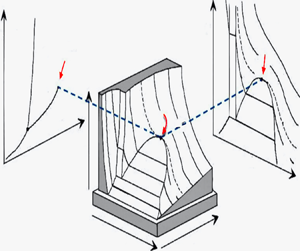
The evolution of the temperature profiles in the bulk and boundary layers is illustrated in figure 6, where the temperature is plotted against position at different times. Since the profiles in the boundary layers are obliterated over the range 0 < x < 1 (middle sections of figure 6), they are shown over a small x range near the top and bottom walls in the left and right sections of the figure, respectively. Figure 6(a) shows a wider perspective over the range $0 \lt t^{\prime} \lt 25\;\textrm{s}$, whereas figure 6(b) depicts the details for $5 \lt t^{\prime} \lt 25\;\textrm{s}$.

Figure 6.

Temperature profiles at the piston-effect time scale against position x. Profiles shown for $0 \lt t^{\prime} \lt 25\;\textrm{s}$ in (a), and for $5 \lt t^{\prime} \lt 25\;\textrm{s}$ in (b). The bulk region is shown for $0.09 \le x \le 0.91$, along with the corresponding boundary layers. The wall temperature ${T^{\prime}_w}$ corresponds to the (−20 mK) horizontal line. The conditions are the same as at the acoustic time scale except that the thermal quench here is 20 mK. Dotted lines correspond to zero gravity and plain lines to an acceleration of 10 g.

We have also added the profiles corresponding to a zero acceleration (dashed lines). In all three regions, the temperature drops significantly with time, especially initially. The profiles in the middle section of figure 6(a,b) reflect the behaviour in the bulk region. We first observe that the temperature gradient ${\textstyle{2 \over 3}}A{\gamma _0}$ is constant and independent of time. There are two contributing terms in (4.13) to the temperature perturbation, the first term ${\textstyle{2 \over 3}}A{\gamma _0}(x - {\textstyle{1 \over 2}})$ represents the coupling between the imposed acceleration and the pressure gradient. The second term ${\textrm{e}^{{\beta ^2}\tau }}erfc(\beta \sqrt \tau )$ is the signature of the piston effect in the heat transfer process. It is positive and monotonically decreasing with time. The profiles are comparable to those numerically calculated by Sharma, Erriguible & Amiroudine (Reference Sharma, Erriguible and Amiroudine2017a,Reference Sharma, Erriguible and Amiroudineb).

The transient behaviour becomes evident in the limits of small and large times. For this, we note the following useful asymptotic forms of the transient term, which will be used in subsequent discussions:

(4.14) \begin{equation} \textrm{e}^{{\beta ^2}\tau}erfc(\beta \sqrt \tau ) \approx \begin{cases} 1 - \dfrac{2}{{\sqrt {\rm \pi}}}\beta \sqrt \tau ,&(\tau \ll 1)\\ \dfrac{1}{{\beta \sqrt {{\rm \pi} \tau } }},&(\tau \gg 1)\end{cases}\end{equation}

Consequently, (4.13) and (4.14) suggest that, in the absence of an imposed acceleration $(A = 0)$, the temperature will everywhere always be larger than the wall temperature ${T_w} = {T_i} - \delta T$, and this case represents the usual process of heat diffusion, with the pressure remaining independent of the position across the three regions and below the initial pressure at all time as per (4.12). Simultaneously, the temperature is independent of the position (flat dashed lines in the middle section of figure 6) with narrow boundary layers. Now, for $A \ne 0$, there is a competition between the acceleration and the piston-effect thermal quench. It is clear from (4.14) that the temperature can be below that of the wall only in the upper half-region (x < 1/2); $T(x \gt 1/2,\tau ) \gt {T_w}$ at any time. The early sharp drop in the bulk temperature depicted in figure 6(a) is reflected in the first equation of (4.14). The saturation shown in the figure at the later time is reflected in the second equation of (4.14) through the $1/\sqrt \tau $ behaviour. In this case, the effect of the thermal quench, despite its imposition at the walls, is no longer felt across the bulk region. The monotonic decrease with time reflected in figure 6 and (4.13) is typical of the bulk region, and will not always be present near the walls. The profiles reveal that the temperature decreases below the boundary value at a longer time ($t^{\prime} \simeq 25\;\textrm{s}$ in figure 6, the piston-effect time scale) near the upper wall of the cell. More generally, this time may be estimated from (4.14) to be: $({\rm \pi} /4{\beta ^2}){(1 - {\gamma _0}/3a)^2} \lt {\tau _{PE}} \lt 9{a^2}/{\rm \pi} \gamma _0^2{\beta ^2}$.

Concerning the complex dynamics near the walls, additional insight is gained by examining (4.7) and (4.10) for small z and z*, respectively. In this case, the analytical inversion becomes possible. Noting that ${L^{ - 1}}[{(s + \beta \sqrt s )^{ - 1}}] = {\textrm{e}^{{\beta ^2}\tau }}erfc(\beta \sqrt \tau )$, we obtain

(4.15)\begin{gather}T(z \to 0,\tau ) \approx {T_w} - \sqrt K \left[ {\frac{{{\gamma_0}A - 3\delta T}}{{3\sqrt {{\rm \pi} \tau } }} + \delta T\beta \,{\textrm{e}^{{\beta^2}\tau }}erfc(\beta \sqrt \tau )} \right]z,\end{gather}

(4.16)\begin{gather}T({z^\ast } \to 0,\tau ) \approx {T_w} + \sqrt K \left[ {\frac{{{\gamma_0}A + 3\delta T}}{{3\sqrt {{\rm \pi} \tau } }} - \delta T\beta \,{\textrm{e}^{{\beta^2}\tau }}erfc(\beta \sqrt \tau )} \right]{z^\ast }.\end{gather}

Figure 6 indicates that while the temperature drops everywhere like $1/\sqrt \tau $ at a significant rate initially. The early behaviour is reflected from (4.15) and (4.16) in the sharp slopes near the walls as the term involving $1/\sqrt \tau $ is dominant for small $\tau$. At a later time, on recalling (4.14), the effect of the quench is annihilated in (4.15) and (4.16) as the terms proportional to $\delta T$ cancel out, yielding a temperature slope essentially equal to $- A({\gamma _0}/3)\sqrt {K/{\rm \pi} \tau }$ near both walls, a behaviour that also explains the saturation with time shown in figure 6 near the two walls. More importantly, (4.16) confirms, as figure 6 indicates, that a sink zone cannot form near the bottom wall for short and long time. On the other hand, a sink zone can form near the top wall. The temperature can drop by an amount essentially equal to $A({\gamma _0}/3)\sqrt {K/{\rm \pi} \tau }$ that subsides over the piston-effect time scale, independently of the thermal quench level.

This result is similar to the experimental observations of Beysens, Fröhlich & Garrabos (Reference Beysens, Fröhlich and Garrabos2011) in which an internal heat source is applied in a cell containing a SCF with thermostated walls (see figure 1). A hot boundary layer compresses (heats) the bulk fluid, and a cold boundary layer expands (cools) the bulk fluid. When the heating stops, the pressure ceases to rise due to the cold layer. However, the pressure drop due to the cold layer still continues as the layer slowly vanishes by diffusion. This results in a temperature drop in the bulk sample that can be reached beyond the initial equilibrium temperature as can be seen from figure 1 (Beysens, Fröhlich & Garrabos Reference Beysens, Fröhlich and Garrabos2011). The effect is more important when the cold boundary layer is thinner, making the heat exchange more efficient. This is especially true when the cold boundary layer is convected by buoyancy due to the presence of the acceleration. The cooling effect is then more pronounced when the acceleration is larger. Our theoretical results corroborate well this experimental study. Moreover, our predictions are in agreement with the numerical results (Sharma, Erriguible & Amiroudine Reference Sharma, Erriguible and Amiroudine2017a,Reference Sharma, Erriguible and Amiroudineb).

Figure 7 shows the evolution of the temperature field as a function of time over both boundary layer and bulk regions. As can be seen from this figure, the top boundary exhibits a negative temperature (the temperature dips below the imposed wall temperature, which in this case is ${T^{\prime}_w} = {T^{\prime}_i} - \textrm{ }20\;\textrm{mK}$). A minimum temperature, similar to the one observed by Beysens, Fröhlich & Garrabos (Reference Beysens, Fröhlich and Garrabos2011) reported above in figure 1, is also predicted and the time at which this minimum temperature occurs increases with the increase in distance from the top wall. On the other hand, the bottom boundary layer does not exhibit a minimum. The presence and absence of the minimum near the top and bottom walls, respectively, can be confirmed from (4.15) and (4.16). Approximately, for a short time and close to the top wall, (4.15) suggests, after using (4.14), that the minimum occurs at a time $\tau \simeq (3a - {\gamma _0})/6a{\beta ^2}$.

Figure 7.

Temperature profile at a fixed z as a function of time (a) in the left boundary layer and (b) in the right boundary layer. The conditions are the same as in previous plots.

4.4. The mechanism behind the sink-zone formation

We are now in a position to elucidate the physical mechanism behind the temperature drop. To aid the discussion, we also include contour and surface plots in figure 8 for the temperature as function of time and position. We recall that the acceleration is acting downward in the x-direction (see figure 3). The heavier fluid in the top thermal boundary layer and the bulk exerts a force (due to its self-weight) on the fluid beneath it, which leads to a high stratification of the density field in the whole domain (due the high compressibility). Consequently, the fluid is compressed near the bottom, while near the top the fluid expands in addition to the usual expansion caused by the piston effect. Therefore, the overall temperature profile is a superimposed effect of the expansion of fluid due to the piston effect and compression or expansion due to the self-weight, depending on the location of the fluid element from the bottom. This results in the temperature near the bottom being higher than in a weightlessness condition, as can be clearly seen from 6 and 8 (the temperature is higher than −20 mK). At subsequent times, as the temperature of the fluid in the thermal boundary layer drops due to cooling, the density in the thermal boundary layer increases while the thermal expansion (contraction in the present case) increases (due to its diverging behaviour when approaching the critical point). While the fluid in the bottom thermal boundary layer is already in a stable configuration, with cold and heavier fluid being under the lighter bulk fluid, the scenario is the opposite for the fluid in the top thermal boundary layer. A heavier and colder fluid (in the top thermal boundary layer) not only compresses the fluid beneath it but also moves downwards, causing the temperature to drop at a faster rate as compared to the weightlessness condition. The combined action of compression of the bulk fluid by this heavy fluid and action of self-weight causes a faster decrease in the temperature near the top as compared to the bottom. Consequently, while the temperature of the fluid near the top reaches the wall temperature, the fluid near the bottom is yet to attain the imposed wall temperature and thus continues to expand. This temperature gradient near the bottom, which corresponds to the temperature in the bulk (and it is constant, as can been seen from figure 6), thus causes the fluid to expand, thereby decreasing the temperature everywhere. As a result, the temperature near the top wall falls below the boundary value and extends into the bulk fluid with time as can been seen in figures 6 and 8). The temperature of the fluid continues to fall below the wall temperature until the fluid in the thermal boundary layer starts to expand due to the heating from the top wall and thus exerting an opposite effect, i.e. compressing the bulk fluid.

Figure 8.

Temperature contour plot (a) and surface (b) as a function of the time and position at the piston-effect time scale. The thermal quench is 20 mK.

When both these opposite effects (the expansion and compression of the bulk due to the bottom and top boundary layers, respectively) become balanced, the temperature stops falling below the boundary value. Subsequently, it tends to return to the imposed values as imposed by the boundary conditions (see figure 7).

5.1. At the acoustic time scale

Perturbing about the initial values, exactly as in (3.2) for a van der Waals gas, yields the following equations:

(5.1a–d)\begin{equation}{\bar{\rho }_t} ={-} {\bar{u}_x},\quad {\bar{u}_t} ={-} \frac{1}{{{\gamma _0}}}{\bar{P}_x} + H(t),\quad - ({\gamma _0} - 1){\bar{u}_x} = {\bar{T}_t},\quad \bar{P} = \bar{\rho } + \bar{T}.\end{equation}

Interestingly, the flow and temperature fields are coupled to the density, which is not the case for a van der Waals gas, as equation (3.3a–d) suggests. In this case, the equation and solution for the velocity in the bulk region take the same form as (3.4) and (3.5) with c = 1, as expected. The temperature takes a slightly different form from (3.5)

(5.2)\begin{equation}\bar{T}(x,s) = \frac{{{\mathrm{\gamma }_0} - 1}}{{{s^2}}}\left( {\frac{{{\textrm{e}^{sx}}}}{{1 + {\textrm{e}^s}}} - \frac{{{\textrm{e}^{ - sx}}}}{{1 + {\textrm{e}^{ - s}}}}} \right).\end{equation}

As in the case of a van der Waals gas, the behaviour is oscillatory in time. The time average over one cycle also suggests, as does (3.7), a linear increase with position

(5.3)\begin{equation}\langle \bar{T}\rangle = ({\mathrm{\gamma }_0} - 1)\left( {x - \frac{1}{2}} \right).\end{equation}

Setting $z = x/\delta $, and noting that the boundary layer thickness is $\delta = \sqrt \varepsilon $ for a perfect gas, the field perturbation takes a slightly different form than (3.8)

(5.4)\begin{equation}\left. \begin{gathered} {\rho (z,t) = 1 + A\hat{\rho }(z,t),\quad u(z,t) = A\sqrt \varepsilon \hat{u}(z,t),}\\ {T(z,t) = {T_i} + A\hat{T}(z,t),\quad P(z,t) = 1 + A\hat{P}(z,t).} \end{gathered} \right\}\end{equation}

We see that the density perturbation for the perfect gas in the boundary layer differs from that of a near-critical fluid. This is discussed later. The density is of order A in (5.4), which is small relative to the supercritical case for a van der Waals gas for which (3.8) indicates that the density is of the order $A/\mu $. Recall that A and $\mu $ are of the order of ${10^{ - 5}}$ and ${10^{ - 3}}$, respectively. The corresponding equations are

(5.5a–d)\begin{equation}{\hat{\rho }_t} ={-} {\hat{u}_z},\quad {\hat{P}_z} = 0,\quad {\hat{T}_t} ={-} ({\gamma _0} - 1){\hat{u}_z} + \frac{{{\gamma _0}}}{{P{r_0}}}{\hat{T}_{zz}},\quad \hat{P} = \hat{T} + \hat{\rho }.\end{equation}

When compared to (3.9a–d), we see that (5.5a–d) suggests that the transient term in the energy equation is no longer negligible for a perfect gas. However, the resulting temperature equation remains of the same form as (3.12), namely ${\hat{T}_t} = (1/P{r_0}){\hat{T}_{zz}} + (({\gamma _0} - 1)/{\gamma _0}){\hat{P}_t}$.

5.2. At the diffusion time scale

The diffusion time scale in a perfect gas is defined by $\tau = \varepsilon t$ where $\varepsilon $ is the same small parameter as defined in § 2 below (2.5). In this case, all field perturbations in the bulk region are of order A, with the corresponding equations written as

(5.6a–d)\begin{equation}{\bar{u}_x} = 0,\quad {\bar{P}_x} = {\gamma _0}H(\tau ),\quad {\bar{T}_\tau } = \frac{{{\gamma _0}}}{{P{r_0}}}{\bar{T}_{xx}},\quad \bar{P} = \bar{\rho } + \bar{T}.\end{equation}

In this case, and despite the presence of a pressure gradient, the velocity is negligibly small over the entire domain. In addition, the diffusive term in the energy equation ensures that the temperature perturbation satisfies: $\bar{T}(x = 0,\tau ) = \bar{T}(x = 1,\tau ) ={-} a\delta (\tau )$ at the two walls.

Consequently, and as expected, there is no formation of thermal boundary layers. In this case

(5.7)\begin{equation}T(x,s) = {T_i} - \delta T\frac{{{\textrm{e}^{x\sqrt {(P{r_0}/{\mathrm{\gamma }_0})s} }} + {\textrm{e}^{(1 - x)\sqrt {(P{r_0}/{\mathrm{\gamma }_0})s} }}}}{{s(1 + {\textrm{e}^{\sqrt {(P{r_0}/{\mathrm{\gamma }_0})s} }})}}.\end{equation}

The above equation reveals that at no time the temperature in the bulk falls below 1 – a. This means that no quenching is observed in perfect gases.

Figure 9 shows the temperature profile as a function of time. The conditions are the same as in the previous SCF case, i.e. the fluid is at 0.2 K above the critical temperature and the applied thermal quench is 20 mK. As expected, no formation of sink zones is predicted.

Figure 9.

Temperature profiles at the diffusion time scale for the perfect gas. The lower dashed line represents the wall temperature.