

1 Introduction
Current and expected demographic and economic trends are likely to jeopardize the financial sustainability of the French retirement pension scheme, which mainly operates on a pay-as-you-go basis. The old-age dependency ratio (population aged 60 and above as a percentage of the population aged 20–59), currently standing at 0.4, is expected to reach 0.69 by 2050, and the deficit of the basic pension scheme is forecast to top at least EUR20 billion by 2020 (COR, 2007), despite the recent parametric reforms adopted in the Pension Reform Act (Loi 2003–775 du 21 aoÛt 2003). Standing at 12.8% of GDP in 2004, pension spending is expected to increase to 13.7% in 2020, and 14.8% in 2050 (European Commission, 2006: 87).
Besides the parametric reforms concerning the pay-as-you-go basic pension scheme, the 2003 Pension Act introduced some fiscal incentives to the development of pension vehicles based on individual and collective funding (PERP and PERCO). But the Pension Reserve Fund (Fonds de réserve pour les retraites, FRR) also provides a funding device.
Created in January 1999, the FRR was designed to sustain the first pillar pension scheme. At the outset, it has been assigned the objective of accumulating 150 billion euros until 2020 and using the cumulated reserves to buttress the first pillar within the next three decades. This cumulating profile was assumed to follow the demographic hump linked to the retirement of the massive baby-boomer cohorts. The FRR thus has a smoothing rather than a structural objective of permanent funding. However sensible this objective is, the FRR suffers from a major drawback, its resources being random for their major component. In fact, its main resources are not levied on a stable basis. As it was enacted in Sweden, the French legislator could have created a supplementary pension contribution on wages to back up the FRR. The purpose of this paper is to estimate the optimal path for pension contribution rates (and the associated evolution of the FRR) necessary to keep the general pension scheme sustainable at the 2050 horizon under a set of demographic, institutional, economic and financial assumptions.
The paper is organized as follows. Section 2 presents an overview of the FRR and the related literature. The general methodology is explained in Section 3. Section 4 reviews the main assumptions and presents the data. Results are given in Section 5. Section 6 concludes.
Overview of the FRR and related literature
Set up in January 1999 by the socialist Government led by Lionel Jospin, the Pension Reserve Fund has been designed to introduce some funding in the pay-as-you-go basic pension schemes, namely the schemes for private sector workers (Régime général de la Caisse Nationale d'Assurance Vieillesse), and for workers of the so-called ‘aligned’ regimes (régimes alignés: MSA, CANCAVA and ORGANIC Footnote 1). These first-pillar pension schemes cover about 80% of workers in France, the remaining 20% being civil servants and workers affiliated to special regimes (public enterprises).
At the origin, the Pension Reserve Fund was financed by the surpluses of the Fund for Old Age Solidarity (Fonds de solidarité vieillesse) and a ‘social solidarity’ contribution levied on companies, with an initial endowment of EUR 300 million, and further proceeds of future privatizations and restructuring of savings banks estimated at EUR 1.5 billion. In 2000 and 2001 the Social Security Funding Act (Loi de financement de la Sécurité Sociale) extended the resources of the FRR including: the surpluses from the general pension scheme, part of the 2% tax levy on capital revenues, and the proceeds of the UMTS auctions. The reserves were to be invested in the financial markets and managed by the Government.
On April 2001, the Pension Reserve Fund has been transformed by the conservative Government led by Jean-Pierre Raffarin into an independent public management body. The reformed body's mandate was to accumulate funding until 2020 to buttress the basic pension scheme. The cumulated funding was then expected to be spent over the period up till 2040 to smooth the demographic hump associated with the massive baby-boomer generation. The 2001 bill set up a monitoring committee made up of 20 members of Parliament and representatives of social partners and the Government, and a directorate composed of three members appointed for a six-year term. The Caisse des dépôts et consignations (a financial institution controlled by the Parliament) was entrusted with the administrative management of the FRR, the financial management being allocated by auction to independent institutional investors in July 2003.
The 2001 bill did not address a widespread criticism concerning the funding of the FRR, namely its random, piecemeal, and unstable resources. Indeed, the bill could have created a supplementary pension contribution on wages to back up the FRR.
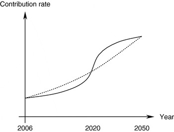
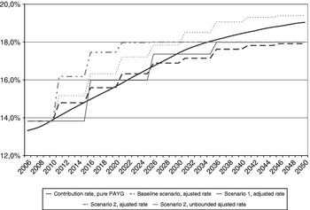
For the sake of argument, let us assume that the FRR has not been created and that the Government aims at balancing the amount of pensions to contributions each year, other things being equal (namely holding constant the retirement age and the replacement ratio). Due to the dramatic expected decrease of the contributor/pensioner ratio between 2005 and 2030, this is likely to induce a very sharp increase in the contribution rate in order to meet the balanced budget requirement during the same period. Let us call ‘pure PAYG contribution rate’ the (theoretical) contribution rate that equalizes the amount of pensions to contributions at each date (represented on the solid curve in Figure 1).
The smoothing of contribution rates

With the implementation of the FRR, the evolution profile of the contribution rate can be more progressive, the reason being that there may exist an intertemporal trade-off between early and delayed increases in the contribution rate. As far as the working-age population is still large until 2020 (the post-World Ward II baby-boom ended in 1964 in France) and the retirees are not so numerous until 2010, the contribution rate can be increased above the pure PAYG contribution rate in the near future (say 2020), the increase being smoother beyond 2020 with a contribution rate below the pure PAYG rate after that date (see the dotted curve in Figure 1). The ‘overincrease’ in the contribution rate enables funding in the FRR until the date at which the two curves intersect. The FRR is thus viewed as a transitory device to smooth the adverse consequences of the demographic baby-boom hump. The idea is to increase the contribution rate above the level needed to balance the public pension scheme accounts while the contributor/pensioner ratio is still high, and then to switch to a lower level when this ratio becomes unfavourable. Smoothing the contribution rate thus means moving from a steep profile (solid curve) to a flatter profile (dotted curve).
This question was addressed in an earlier paper (Berger and Lavigne, Reference Berger and Lavigne2004) where we aimed at minimizing the year-by-year increase of the contribution rate, subject to: (i) the equation of evolution of the reserve fund viewed as the state-dependant variable; (ii) an initial and a terminal condition on the reserve fund level; (iii) a non-negativity constraint on the reserve fund level. This methodology first initiated by Vernière (Reference Vernière1999) assumes that the purpose of the FRR is to minimize the year-by-year increase of the contribution rate. It follows that the actual contribution rates would have to be changed every year, which seems fairly unrealistic since changes in contribution rates are costly.Footnote 2 In the present paper, we take into account this drawback and we introduce a fourth constraint: the number of contribution rate changes is limited over the simulation period (or equivalently, we impose a minimum number of years between two changes in the contribution rate).
A recent report by the Conseil d'Orientation des Retraites provides other simulations of the French Pension Reserve Fund (COR, 2006). It assumes that the FRR cannot get extra resources through increases of the contribution rate in the first pillar. The main funding comes from the surpluses of the Fonds de Solidarité Vieilliesse, an assumption which is extensively discussed in the COR report.Footnote 3 Under the rather optimistic assumption of an unemployment rate equal to 4.5% beyond 2015, the COR simulations show that the FRR accumulates 127 billion euros in 2020; under the pessimistic assumption of a 9% unemployment rate beyond 2015, the amount in FRR would be equal to 67 billion euros; an intermediate assumption of 7% unemployment rate over the same period leads to an expected amount of 84 billion euros. This range of results clearly shows that a more perennial source of funding is needed to isolate FRR from erratic unemployment conditions.
2 Methodology
This section presents the general methodology of our simulation programme. As in our previous contribution (Berger and Lavigne, Reference Berger and Lavigne2004), we assume that the objective of the FRR manager is to minimize the increase in the contribution rate over the whole period of simulation.
The optimization programme can be written as
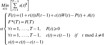
with:
- c
adjusted contribution rate (or ‘funded pay-as-you-go’ contribution rate) – endogenous
- F
Pension Reserve Fund – endogenous
- F*
targeted Pension Reserve Fund – exogenous
- P
pensions – exogenous
- W
wages on which are levied pension contributions – exogenous
- r
real return on portfolio – endogenous
- A
lump-sum contributions – exogenous
- λ
length (in years) of contribution step – exogenous parameter
The first constraint is the evolution equation of the FRR. The second equation is the terminal condition; since we impose a terminal condition on F(T), we have chosen not to minimize the last jump in the contribution rate. It means that there could exist a jump in the adjusted contribution rate in year T+1 if the fund is exhausted in year T. The third equation is the non-negativity constraint on the FRR. The fourth constraint states that the contribution rate cannot jump if the time elapsed since the previous jump is inferior to λ; put differently it means that there is at least λ years between two changes in the contribution rate. We have thus chosen to call c the ‘adjusted’ contribution rate instead of the ‘smoothed’ contribution rate to underline the fact that the contribution rate profile is still flatter, although piecewise adjusted, than the pure PAYG contribution rate profile.
Since this optimization programme cannot be analytically solved with a closed-form solution, we used an algorithmic solution of the following programme
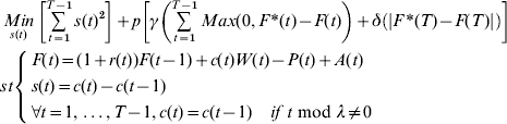
with:
- γ, δ
weights of the different objectives – exogenous parameters
- ρ
optimization step – exogenous parameter
We are aware that taking γ and λ as exogenous parameters does not lead to the theoretical optimal solution. Nevertheless taking a wide range of values for the parameter ρ can give an acceptable approach to the solution for this programme. For the simulations, the optimization step ρ has been fixed such as ρ∊[0.001, 100]. The γ, δ parameters have been set at 100 and 1,000 respectively. Starting from an initial ρinitial=ρ1, a vector of optimal contribution rates  is determined for the whole period of simulation, jointly with the value of the optimal step in the contribution rate. The same values are then determined for ρ2. is compared with
 , the smallest value being kept and compared with the next one until ρfinal.
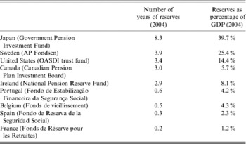
The simulations are run on annual basis from 2006 to 2050. The year 2050 has been chosen as the final year of simulation with respect to the expected extinction of the last baby-boom cohorts. To keep in line with the statutory objective of a transitory accumulation of funding during the next two decades and an exhaustion of the FRR in 2050, most of our simulations are consistent with this objective. Other simulations have been performed assuming a structural funding for the FRR. Such a structural objective has been assigned to some pension reserve funds in other countries, mainly countries in which pension reserve funds were created long ago (e.g. Japan, Sweden, and United States). Table 1 presents some basic statistics on pension reserve funds in a selected number of countries. These figures are not quite comparable since the reserve funds have not the same perimeter, ranging from an extensive coverage of all pillars (Japan) to the coverage of the sole PAYG private sector pillar (France). For our simulations, we have assumed a structural objective of three years of pension benefits for the final size of the FRR.
Pension reserve funds in a selected number of countries

Source: Vernière (Reference Vernière2005).
3 Main assumptions and data
The simulation programme is made of three modules: demographic, economic, and financial. These modules have some exogenous data, some of them being preset, others being chosen by the programme user. All economic and financial variables are in real terms: introducing a projected inflation rate is irrelevant since our main objective is to forecast contribution rates for the future.
Demographic data and projections
Data and projections of population come from INSEE (2002). Since the FRR is designed to cover only the pensioners of the basic pension regimes (régime de base and regimes alignés), the population under simulation represents 80% of the total population. Mortality rates, fertility rates, and immigration have been projected along three sets of scenarios (baseline, optimistic, pessimistic).
The baseline assumption regarding mortality consists in extrapolating the observed mortality rate over the past 30 years for the next 50 years. The low mortality assumption consists in accelerating the reduction of the mortality rate of the elderly: the life expectancy would reach 86 for men and 94 for women in 2050. Under the high mortality assumption, life expectancy would be equal to 82.6 and 87.7 respectively.
In the baseline scenario, the fertility rate is set at 1.8 children per woman until 2050 (its value over the past two decades). Starting at 1.8 in 2006, it is set at 2.1 from 2015 until 2050 in the optimistic scenario and at 1.5 in the pessimistic scenario over the same period. As regards immigration, the baseline scenario retains an inflow of 50,000 persons per year; in the optimistic and pessimistic scenarios, the inflows are 100,000 and 0 respectively.
Institutional and economic data
Institutional and economic data are crucial for the funding of the FRR. For the simulations, we set an ‘over-contribution rate’ on the wage bill. We therefore need some assumptions on projected employment rates.
Gross replacement rate
Our simulations rely on the gross replacement rate of the basic pension regime. It is very difficult to forecast the evolution of replacement rates over a 50 year horizon since these rates are conditioned by the individuals' labour supply behaviour and career on the one hand, and by institutional features on the other hand (number of years of career taken into account to compute the reference wage, minimal length of the contributory period, level of full replacement rate and so on … ). We have thus considered complete careers and set the replacement rate equal to its current level of 50% of the gross reference wage for the total simulation period (computed on the best ten years of career before 1993, and progressively on the best 25 years of careers after the 1993 Pension Reform Act). The gross reference wage is computed under the social security ceiling: we have assumed that the social security ceiling increases along with labour productivity as it has in the past. We have computed the replacement rate for direct rights (i.e. the rights to pension for a given pensioner), but also for indirect rights (survivor's benefits) since the basic pension regime provides a pension for widows equal to 54% of the direct pension (under conditions linked to overall household's resources).
Legal retirement age and length of contributory period
In our simulations, we have set the retirement age at its legal minimum value. For the length of contributory period needed to be entitled to a full replacement rate, we have taken into account the past pension reforms. Before 1993, it was equal to 37.5 years. After the 1993 pension reform act, it has been progressively increased to 40 years. With the 2003 reform, it will progressively increase to 41 years.
Employment rate
Our simulations are based on the projections of employment rates by INSEE (2002). In the baseline scenario, the unemployment rate is set to 8.9% (its level in March 2002). Three other scenarios are considered: an increase in female labour force participation (the French female employment rate reach the level currently observed in Sweden for the 30–54 age group); a low unemployment rate (the unemployment rate progressively declines to 5% until 2010, and then remains stable at this level until 2050); an increase in the length of employment period over the life-cycle (a five-year increase in the current employment rate profiles).
Wages and labour productivity
The wage bill has been forecasted using an initial structure by professional status and gender in 2004 (Pouget and Skalitz, Reference Pouget and Skalitz2006). Since we have run macro-projections, we have not used age–earnings profiles. Indeed age–earnings profiles are increasing mostly above the Social Security ceiling, and we have taken into account only the fraction of wage under this ceiling. The distribution of wages across the population is maintained constant over the simulation period. We have assumed a constant growth of labour productivity over the simulation period; the growth of labour productivity is also assumed to be the same across the different categories of workers. In the baseline scenario, the growth of labour productivity is set to 1.3% (its average level over the past 20 years). In the optimistic scenarios, it is set to 1.8%, and in the pessimistic ones to 0.7%.
Initial ‘over-contribution rate’ and maximal contribution rate
Our programme runs with an initial over-contribution rate and a maximal contribution rate over the simulation period. In the baseline scenario, the over-contribution rate is set at 0.5 point and the maximal rate at 18%. For the optimistic (resp. pessimistic) scenarios, these values have been set at 0.25 (resp. 0.75) and 16% (resp. 22%).
Financial data
Simulations without shocks on the financial markets
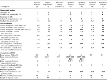
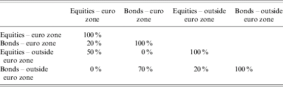
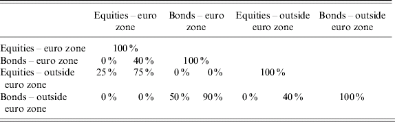
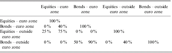
The 2001 bill has imposed some rules on the allocation of the Pension Reserve Fund portfolio: 38% in equities of the euro zone, 17% in equities outside the euro zone, 38% in bonds of the euro zone, and 7% in bonds outside the euro zone. We have thus four categories of securities in which the FRR portfolio can be invested. For each category of securities, the programme user chooses the forecasted return and risk for the whole simulation period. In the baseline scenario, the return and risk have been set according to the observed values on the past 50 years (see table 2). Isolating financial variables from demographic trends is indeed a limit of our exercise. But there is a controversy on the validity of the ‘asset meltdown hypothesis’ according to which financial asset prices could decline as the share of households over the age of 65 increases. The correlation matrix of returns between the four categories of assets is also set by the programme user: it has been assumed to be constant whatever the scenario (see tables 3 and 4).
Assumptions in the different scenarios

Notes: (a) mortality: assumption 1: mortality trend observed over the past 30 years projected on the next 50 years; assumption 2: deceleration in the reduction of the mortality rate of the elderly: the life expectancy would reac h 82.6 for men and 87.7 for women in 2050; assumption 3: acceleration in the reduction of the mortality rate of the elderly: the life expectancy would reach 86 for men and 94 for women in 2050.
(b) fertility and immigration (joint hypothesis): assumption 1: 1.8 children per woman et 50,000 immigrants per year; assumption 2: 2.1 children per woman from 2015 and 50,000 immigrants per year; assumption 3: 1.5 children per woman and 50,000 immigrants per year; assumption 4: 1.8 children per woman et 100,000 immigrants per year; assumption 5: 1.8 children per woman and 0 immigrants per year.
(c) labour force participation: assumption 1: unemployment rate equal to 8.9%; assumption 2: increase in female labour force participation (the female employment rate progressively reaches the level currently observed in Sweden for the 30–54 age group); assumption 3: low unemployment rate (the unemployment rate progressively declines to 5% until 2010, and then remains stable at this level until 2050).
Correlation matrix of the returns on four classes of securities (baseline scenario)
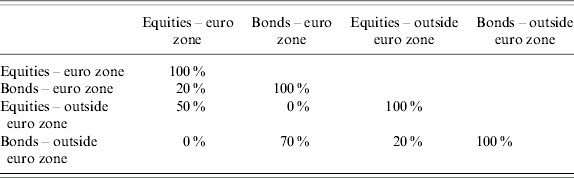
Correlation matrix of the returns on four classes of securities (optimistic scenarios: left; pessimistic scenarios: right)
Stress tests on financial performances
The preceding set of simulations has been enriched by stress tests to take into account random but plausible shocks on financial markets. These tests enable to assess the robustness of our results and to measure the sensibility of the FRR to unexpected low returns and risk increases.
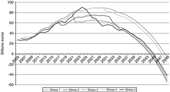
• Stress test 1: we simulate the consequences of a 10% loss of the FRR portfolio during he year in which it has accumulated its maximal amount of reserves;
• Stress test 2: we impose a random 10% loss of the FRR portfolio on each period of ten years; on the 45 years of simulation we therefore have 5 losses of 10% on the return of the FRR portfolio;
• Stress test 3: in this test we take into account a 20% loss due to exchange rate according to the same principle as in stress test 1. The loss is limited since the total exposure to foreign exchange risk is limited to 24% by the 2001 bill.
• Stress test 4: this test takes into account a progressive and steady modification of the correlation matrix between returns on the four classes of securities. 100,000 simulations are run and the worst is retained.
• Stress test 5: this test assumes a perfect correlation across returns of the four classes of securities. In other words, the FRR portfolio is no longer diversified. This stress test enables to measure the impact of portfolio diversification on the cumulated reserves of the fund and the associated contribution rates.
These stress tests can be performed in any scenario; in what follows, for length reason, we only present the results of stress tests applied to the baseline scenario.
4 Results
We first present the results of the simulations in the central scenarios assuming the same values for the demographic, economic, and financial modules. We then turn to optimistic and pessimistic scenarios.
Simulations under central scenarios (Figures 2 to 5)
Baseline scenario
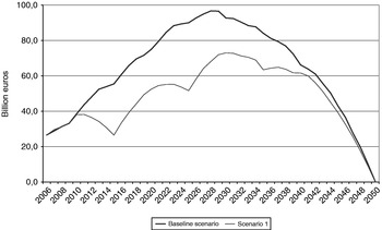
In the baseline scenario (the length between two changes in the contribution rate is equal to five years), the pure PAYG contribution rate steadily increases from 13.3% to 19.0% (Figure 2). The pure PAYG contribution rate is below the adjusted contribution rate until 2023 where it reaches 16.2%. Between 2026 and 2050, the adjusted contribution rate jumps from 16.9% to 17.9% (slightly less than the binding maximum contribution rate). The evolution of the FRR is characterized by an unsteady growth until 2028 where the fund reaches its maximal value equal to 96.7 billion euros (Figure 3).
Contribution rates, central scenarios

Evolution of the pension reserve fund, central scenarios

Ten-year step scenario
When the length between two changes in the contribution rate is equal to ten years instead of five years, the adjusted contribution rate reaches its maximal value in 2046 (scenario 1, Figure 2). The first increase happens in 2016, where the adjusted rate goes from 13.8% to 16.0%. This significant jump enables a less important accumulation of reserves in the fund whose shape is no longer concave (scenario 1, Figure 3).
Structural funding scenario
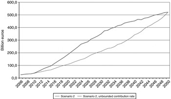
Scenario 2 relies on the same demographic, economic and financial assumptions as in the baseline scenario (see Table 2). The only difference is that we have imposed the accumulation of three years of pension benefits in the fund in 2050. The FRR is thus assumed to have a ‘structural’ objective of introducing permanent funding in the pure pay-as-you-go pension system. To compare the evolution profile of the contribution rate we have first assumed the same upper bound on the adjusted rate as in the baseline scenario (18%). Alternatively, we have assumed an unbounded evolution of the contribution rate. In these structural funding scenarios, the adjusted contribution rates are 0.4 to 2.5 percentage points higher than in the baseline scenario. As expected, when there is an upper bound on the contribution rate, the adjustment heavily penalizes the working generations in the next two decades (Figure 2, scenarios 2). The evolution profile of the FRR is no longer hump-shaped, but monotonously increasing. The FRR ends at 521 billion euros in 2050 (Figure 4).
Evolution of the pension reserve fund, structural objective, scenario 2

Stress tests in the baseline scenario
The stress tests 3 and 4 hardly modify the shape of FRR accumulation (Figure 5). On the contrary, the stress tests 1, 2, and 5 induce a significant drop in the accumulation of reserves in the fund, and the fund is in deficit beyond 2045.
Stress tests on the pension reserve fund, baseline scenario

Optimistic scenarios (Figures 6 and 7)
Optimistic scenarios combine several favourable demographic, economic, and financial assumptions (see Table 2).
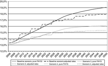
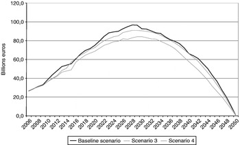
Compared with the baseline scenario, scenario 3 assumes a decelerating life expectancy, a high fertility ratio, an increase in female labour employment rate, a high labour productivity growth, higher financial returns, and lower risks. The fund is also assumed to receive some lump-sum contributions in 2007, 2010, and 2015. The maximum contribution rate is set at 16% (see Table 2). Under these assumptions, the pure PAYG contribution rate steadily increases from 13.2% in 2006 to 16.0% in 2050 while the adjusted rate increases from 13.4% to 14.6% in 2021, the year from which the adjusted rate becomes inferior to the pure PAYG (Figure 6). This upward trend in the optimal contribution rate enables a weaker accumulation in the fund (the cumulated amount is maximal in 2030 and reaches a peak of 84.3 billion euros (Figure 7).
Contribution rates, optimistic scenarios

Evolution of the pension reserve fund, optimistic scenarios

Compared with the baseline scenario, scenario 4 postulates a massive immigration and a low rate of unemployment (steady decrease of the unemployment rate until 2010 and stabilization from then on at a 5% level). The mortality rate, the labour productivity growth, the financial variables, and the lump-sum contributions are set at the same level as in scenario 1 (see Table 2). This scenario 4 is slightly more favourable than the scenario 1 since the pure PAYG contribution rate increases from 13.2% in 2006 to 16.1% in 2050, but the adjusted rate is from 13.4% to 15.3% in 2050 (Figure 6). The cumulated amount in the fund is lower than in the baseline scenario with a maximum equal to 91.0 billion euros in 2028 (Figure 7).
To sum up, the optimistic scenarios enable a moderate adjustment of the contribution rates about 2 to 2.2 percentage points over the simulation period and a slightly lower accumulation of reserves in the FRR.
Pessimistic scenarios (Figures 8 and 9)
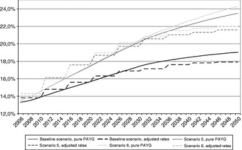
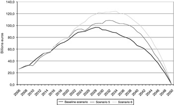
Scenario 5 combines an increase in life expectancy, a low fertility ratio, a weak growth of labour productivity, lower returns and higher risks compared with the baseline scenario (see Table 2). Under these assumptions, the pure PAYG contribution rate would rise from 13.6% to 23.5% (i.e.+9.9 percentage points). Imposing a maximum 22% contribution rate and an initial over-contribution equal to 0.75 point, the adjusted contribution rate sharply increases in the first decadem, which allows an important accumulation of reserves in the fund which tops up to 108.7 billion euros in 2032.
Contribution rates, pessimistic scenarios

Evolution of the pension reserve fund, pessimistic scenarios

Scenario 6 differs from scenario 5 with respect to immigration, which is assumed to be nil, and with respect to fertility ratio which is assumed to be the same as in the baseline scenario. Imposing a maximum 22% contribution rate, the profile of contribution rates is less favourable than the profile exhibited in scenario 5, the adjusted contribution rate reaching its maximum value in 2046. The accumulation of reserves culminates at 123.9 billion euros in 2034.
5 Conclusion and extensions
This paper has presented some simulation results on the projected evolution of the French Pension Reserve Fund under various assumptions. The main idea was to optimize the profile of the trend in contribution rates needed to meet the objective of a balanced basic pension scheme over the period 2006–2050.
When the Pension Reserve Fund was implemented in 1999, the French government expected an accumulation of reserves for an amount of 150 billion euros in 2020 to meet the ‘smoothing objective’ of the fund. Our simulations show that the maximum amount of funding is likely to be less important under plausible assumptions, about 100 billion euros by the end of the 2020s. Stress tests show that only severe shocks on financial markets may dramatically affect the accumulation profile of the FRR.
Let us remember that our model is not intended to simulate the evolutions of the public pension regime per se. Our purpose was to assess the means by which the necessary increase in contribution rates can be adjusted in the future decades in order not to penalize the future generations, ceteris paribus (keeping replacement rates and retirement age constant). Therefore, our demographic, economic, and financial assumptions have to be challenged bearing the ‘adjustment profile’ in mind. Of course, other criteria could be more valuable for policymaking purposes if a more comprehensive concern for public pension schemes sustainability has to be dealt with. In this case, a general equilibrium model is needed with links between labour markets, financial markets, and public finance. More generally, the rates of return on financial assets could be related to demographic trends, because of the well-known ‘asset meltdown hypothesis’.