4.1. A puller leading another puller

When one puller leads another puller, it will eventually come into contact if the initial distance is as large as S ^*(0) = 3. Figure 8 shows the time evolution of the speeds of the two identical pullers ( $\beta$ ₁ = $\beta$ ₂ = 5) at various Reynolds numbers (see also supplementary movie 1 a–c are available at https://doi.org/10.1017/jfm.2025.10679). The speed of a single puller was also included for each Re _s . The general features were similar for all cases considered (figure 8). Both pullers were seen to swim at the same speed at t ^* ≤ t _s , during which neither puller ‘feels’ the existence of the other. Subsequently, the trailing puller speeds up significantly owing to the attraction of the leading puller. In contrast, the speed of the leading puller increased slightly for some time, then decreased sharply because it was attracted by the trailing puller. At t ^* = t _c , both pullers come into contact when the speed of the leading/trailing puller abruptly increases or decreases to a value that is slightly higher than that of a single puller at the same Re _s (figure 8). The reason will be given later in this section. At $t^{*} \gt t_{c}$ , the two pullers formed a stable doublet and swam. Moreover, both times (t _s and t _c ) are larger for a higher Re _s . This is reasonable because the speed of a single puller decreased with Re _s . Another possible reason is that the negative pressure regions of the puller become smaller as Re _s increases (figure 4). Therefore, it takes longer for the pullers to hydrodynamically interact with each other before they touch and form a doublet at a higher Re _s .

Pullers with different strengths ( $\beta$ ) exhibit similar behaviours. To demonstrate this, we varied $\beta$ ₂ ( $\beta$ ₂ = 1, 5, 9) while keeping $\beta$ ₁ unchanged ( $\beta$ ₁ = 5). Our simulations indicate that the pullers always touch each other and form a doublet that swims at a speed dependent on Re _s and $\beta$ ₂. Notably, for each $\beta$ ₂ studied, the speed of the doublet decreased with Re _s and fit well with the solution of a power-law formulation that exhibited a shape similar to that of a single puller of strength $\beta$ ₂ (Khair & Chisholm Reference Khair and Chisholm2014), as shown in figure 9.

Figure 9.

Steady speeds ( $U_g^* = U_{g}/U_{s}$ ) of a doublet consisting of two pullers with $\beta$ ₁ = 5 and (a) $\beta$ ₂ = 1, (b) $\beta$ ₂ = 5, (c) $\beta$ ₂ = 9. Note that we used U _g to represent the steady speed of a group of particles (squirmers and spheres). The dashed lines are the least squares fitting curves. The dash-dot-dotted, solid and dash-dotted lines denote the speeds of a single puller ( $U_a^*$ ) with $\beta$ = 1, 5, 9 (see (3.1)).

According to Khair & Chisholm (Reference Khair and Chisholm2014), the stronger the puller, the slower it swims (figure 3 b). In contrast, a doublet consisting of a stronger puller may exhibit a higher speed (figure 9 c). This tendency is significant at low values of Re _s . For instance, the steady speed ( $U_g^* = U_{g}/U_{s}$ ) of a doublet with $\beta$ ₁ = 5 and $\beta$ ₂ = 1 is approximately 0.74U _s at Re _s = 0.1 (figure 9 a), i.e. $U_g^*$ ≈ 0.74. We use U _g to represent the steady speed of a group of particles (squirmers and spheres), to distinguish it from that of a single particle (U _a ). The value of $U_g^*$ increases to approximately 1.25 when $\beta$ ₂ = 9 (figure 9 c). Figure 10 illustrates the primary reason for this by showing the instantaneous flow fields of the same doublets as those shown in figure 9 at Re _s = 0.1. The most significant differences were observed in the pressure distributions. For $\beta$ ₂ = 1 (figure 10 a), the negative pressure is much more noticeable at the rear of the doublet than at the front. The opposite trend was observed for $\beta$ ₂ = 9 (figure 10 c). Consequently, an additional force originating from the (negative) pressure differences hindered the doublet with $\beta$ ₂ = 1 (figure 10 a) while propelling the other (figure 10 c). This is why a single puller ( $\beta$ = 5) swims faster than the doublet with $\beta$ ₂ = 1 but slower than that with $\beta$ ₂ = 9 for the entire range of Re _s considered.

Figure 10.

Flow fields of the same doublets as those shown in figure 9(a–c) at Re _s = 0.1.

To provide a quantitative analysis, we show the differences in swimming speed between the doublet and single puller ( $\beta$ = 5) in figure 11(a), i.e. ΔU = $U_g^*$ – U _a ^*. The speed of two identical pullers ( $\beta$ ₂ = 5) is always slightly higher than that of a single puller. One possible mechanism is as follows. Squirmers have macroscopic speeds because of the prescribed slip velocity imposed on their surfaces. The surface area of the doublet was twice that of the single puller, indicating that more slip velocity sources contributed to the macroscopic speed of the doublet. Therefore, the doublet was expected to swim much faster than a single puller. However, when the pullers come into contact, the trailing puller faces the rear end of the leading puller, and the puller gains thrust from the front. Consequently, the self-propulsion dynamics of the trailing puller are significantly suppressed (figure 10). These results are further confirmed in § 4.5, which describes a string of multiple pullers that exhibits a slowly increasing speed as the number of pullers increases. This mechanism also applies to doublets with different pullers (figure 9 a,c), for which the fore and aft pressure differences dominate the locomotion of the doublets. Figure 11(a) also shows that the speed of the doublets converges to that of a single puller as Re _s increases. As expected from figure 8, the contact time (t _c ) increases with Re _s , and this finding is further confirmed by figure 11(b). Moreover, it took longer for the trailing puller to chase the stronger puller (figure 11 b). This is rational because a stronger puller runs slower.

Figure 11.

Summarisation for a doublet consisting of two pullers with $\beta$ ₁ = 5 and a varying $\beta$ ₂. (a) Differences in swimming speed ( $ \Delta U = U_{g}^{\ast}$ – $ U_{a}^{\ast} $ ) between the doublets and single puller ( $\beta$ = 5). (b) Contact times of the pullers (i.e. t _c , as indicated in figure 8). Note that the speed of single puller ( $U_a^*$ ) is obtained according to (3.1).

4.2. A puller leading a pusher

The situation is quite different when a puller leads a pusher because the pullers are attractive, whereas the pushers are repulsive, in terms of the fore and aft pressures of the squirmers (figure 4). For instance, figure 12(a) shows that the squirmers do not come into contact at all when Re _s = 0.01, at which point a single pusher ( $\beta$ = −5)/puller ( $\beta$ = 5) swims at the same speed (U _s = 2B ₁/3). Interestingly, the speeds of both squirmers remained the same at all times, and finally reached a value that was substantially larger than U _s (figure 12 a), i.e. $U_g^*$ ≈ 1.55. At a higher value of Re _s , the squirmers may contact and form a stable doublet that swims faster than does a single pusher ( $\beta$ = −5), as seen in figure 12(b,c). Note that supplementary movies 2 a–c accompany figure 12(a–c). Compared with the case of two pullers (figure 8 b,c), it took a much longer time for the puller and pusher to swim because the attractive puller is competing with the repulsion of the pusher all the time before they finally touch. The results in figure 12(b,c) correspond to the initial distances between the squirmers of S ^*(0) = 3. However, similar behaviours would be observed for other initial distances because the trailing pusher ( $\beta$ ₁ = −5) always swims faster than the leading puller ( $\beta$ ₂ = 5) at a non-zero value of Re _s .

Figure 12.

Time histories of the speeds of a leading puller ( $\beta$ ₂ = 5) and trailing pusher ( $\beta$ ₁ = −5) at (a) Re _s = 0.01, (b) Re _s = 0.1, (c) Re _s = 1. See also supplementary movies 2(a–c).

Figure 13.

Terminal speeds of a doublet consisting of a trailing pusher ( $\beta$ ₂ = −5) and leading puller with different strengths: (a) $\beta$ ₁ = 1, (b) $\beta$ ₁ = 5, (c) $\beta$ ₁ = 9. The dashed lines are the least squares fitting curves. The solid line represents the solution for a single pusher with $\beta$ = −5 (Khair & Chisholm Reference Khair and Chisholm2014).

The pressure distributions (figure 4) provide a direct view of how the two squirmers attain an enhanced speed. Generally, the pressure difference force resulting from the negative and positive pressures at the front and rear ends of the squirmers, respectively, acts as an additional thrust on the squirmers for all values of Re _s studied. Note that the trailing pusher gains thrust from the rear. In contrast to the case of two pullers (§ 4.1), it does not matter whether the two squirmers come into close contact or not. Consequently, the doublet can swim as fast as approximately 2U _s at Re _s = 1 (figure 12 c), i.e. $U_g^*$ ≈ 2.

Similar to figure 9, figure 13 summarises the terminal speeds of a structure consisting of a trailing pusher ( $\beta$ ₂ = −5) and leading puller with different strengths ( $\beta$ ₁ = 1, 5, 9). The solution of single pusher with $\beta$ = −5 (Khair & Chisholm Reference Khair and Chisholm2014) was also included. We reveal that the pusher never comes into contact with the weak puller ( $\beta$ ₁ = 1) because the repulsive pusher dominates how the two interact (see figure 15(a) below). For the range of Re _s studied, the speed of the structure with $\beta$ ₁ = 1 increased linearly with Re _s and was slightly higher than that of the single pusher (figure 13 a). In contrast, the pusher always touched the strong puller (figure 14). That is, $\beta$ ₁ = 9, and a remarkably enhanced speed was eventually achieved for all Re _s values (figure 13 c). For instance, a doublet with $\beta$ ₁ = 9 swims more than 100 % faster than a single pusher at Re _s = 0.01. Certainly, a strong puller not only dominates the attraction of the squirmers, but also contributes to the increase in speed. Figure 14 shows that most surfaces of the trailing pusher bear the negative pressure generated by the strong puller that takes the lead, which produces a larger thrust on the doublet. In figure 13(c), a linear relationship between $U_g^*$ and Re _s is also attained for Re _s ≥ 0.4. However, for the intermediate puller ( $\beta$ ₁ = 5), the squirmers maintained an initial distance at all times when Re _s < 0.05 (figure 13 b). We observed an abrupt increase in speed when the pusher caught up with the puller at Re _s = 0.05. Similarly, another linear formulation between $U_g^*$ and Re _s (Re _s ≥ 0.05) was attained for the doublet with $\beta$ ₁ = 5.

Figure 14.

Iso-surfaces of the pressure for a doublet consisting of a leading puller ( $\beta$ ₂ = 9) and trailing pusher ( $\beta$ ₁ = −5) at (a) Re _s = 0.01, (b) Re _s = 0.1, (c) Re _s = 0.5, (d) Re _s = 1.

Figure 15.

Simulation results for the interaction between a leading puller ( $\beta$ ₂ = 1) and trailing pusher ( $\beta$ ₁ = −5). (a) Distances between the squirmers at various values of Re _s . (b) Speeds of both squirmers at two values of Re _s . The inset in (b) shows the iso-surface of the pressure (levels ±0.02) for the squirmers at Re _s = 0.2.

Figure 15(a) shows the time history of the distances between the pusher and weak puller ( $\beta$ ₁ = 1) at various Re _s values. Note that the distances for the strong puller ( $\beta$ ₁ = 9) exhibit similar variations that resemble those shown in figure 7(a) for all values of Re _s studied (not shown here). In contrast, Re _s plays a significant role in the interaction between the weak puller and pusher. The distance between the two increases instantly from an initial value when Re _s is low (Re _s = 0.01, 0.05, 0.2), suggesting that the puller is ‘repelled’ by the trailing pusher (figure 15 a). This is further illustrated in figure 15(b), which shows the time history of the speeds of both squirmers at Re _s = 0.2 and 1. The weak puller attains a speed that is considerably higher than that of the pusher at Re _s = 0.2 before the squirmers swim as a whole. This is in contrast to the case of an intermediate puller ( $\beta$ ₁ = 5) interacting with the same pusher (figure 12 b,c). Ultimately, the weak puller maintains a large distance from the pusher (inset of figure 15 b). However, as Re _s increased, the speed of the pushers increased, whereas that of the pullers decreased (figure 3 b). Therefore, the pusher tends to approach the weak puller at higher Re _s values (figure 15 a). In particular, figure 15(b) shows that the puller swims faster than the pusher for t ^* < 0.5 at Re _s = 1, which leads to an increasing distance. Subsequently, the pusher became faster, and the distance between the two decreased to a constant value (figure 15 a). The repulsive pusher keeps the weak pullers apart from each other.

4.3. A pusher leading a puller

Compared with § 4.2, the situation becomes nearly opposite when a pusher leads a puller. Figure 16(a–c) show the speeds of a leading pusher ( $\beta$ ₂ = −5) and trailing puller ( $\beta$ ₁ = 5) at the same values of Re _s as those shown in figure 12(a–c), representing three types of interacting behaviours. At low values of Re _s (Re _s = 0.01, figure 16 a), the squirmers moved at the same speed, which was approximately one-third of that of the opposite case (figure 12 a), i.e. $U_g^*$ ≈ 0.52. As Re _s increased, the pusher moved faster than the puller. However, at an intermediate value of Re _s (e.g. Re _s = 0.1 in figure 16 b), the leading pusher may swim slowly along with the puller at all times, or at least for a substantial amount of time. The pusher could quickly remove the puller only when Re _s was sufficiently high (figure 16 c).

Figure 16.

Time histories of the speeds of a leading pusher ( $\beta$ ₂ = −5) and trailing puller ( $\beta$ ₁ = 5) at (a) Re _s = 0.01, (b) Re _s = 0.1, (c) Re _s = 1.

The primary reason for the observation in figure 16 is simple: the attractive trailing puller attempted to prevent the leading pusher from leaving. This may succeed at a low value of Re _s . As illustrated in figure 17(a), the positive/negative pressure at the front and rear ends of the squirmers resulted in an additional force that held the doublet back at Re _s = 0.01. The visible expansion of the negative flow between the squirmers (figure 17 b) may reflect the slow speed of the doublet, compared with that of a single puller or pusher at the same Re _s value (figure 4). Figure 17(c) shows the fluid streamlines around the structure in the (x,z) plane. Two circulating regions are known to exist at the front and rear ends of a squirmer. Therefore, four circulating regions exist between the leading and trailing squirmers. When the squirmers approach each other, these four circulating regions incorporate into two larger regions (figure 17 c).

Figure 17.

Simulation results for a doublet consisting of a leading pusher ( $\beta$ ₂ = −5) and trailing puller ( $\beta$ ₁ = 5) at Re _s = 0.01: (a) fluid pressure, (b) streamwise fluid velocity, and (c) the streamlines in the (x,z) plane.

Figure 18.

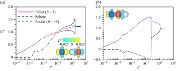
Time histories of the speeds of a leading sphere and (a) trailing pusher ( $\beta$ = −5) or (b) trailing puller ( $\beta$ = 5) at Re _s = 1. See also supplementary movies 3(a,b).

4.4. Interactions between microswimmers and a sphere

Microswimmer-driven cargo transport in biomedical applications has received considerable attention in recent years because of its numerous advantages. Here, we studied how a sphere was driven by squirmers to reveal the dynamic features of active particles interacting with passive particles. The results of this study shed light on the performance of squirmer-driven cargo transport.

As illustrated in figure 18, a sphere can be ‘pushed’ to run by either a pusher ( $\beta$ = −5, figure 18 a) or a puller ( $\beta$ = 5, figure 18 b). However, significant differences were observed between the two cases. Driven by the pusher, the sphere eventually attained a speed (1.37U _s ) that was significantly higher than that of the same sphere (0.17U _s ) driven by the puller. Typically, the sphere exhibited a backward speed owing to the attraction of the puller before it ran as a whole (figure 18 b). In contrast, the sphere accelerated quickly when it interacted with the pusher (figure 18 a). More importantly, it took considerably longer for the pusher and sphere to reach a steady state (figure 18 a). However, once the sphere contacts the puller, the two form a stable doublet and run at a constant speed, similar to the case of two pullers (§ 4.1). Supplementary movie 3 shows the two cases.

From figure 4, it is expected that the sphere eventually contacts the puller while keeping a distance from the pusher (see figures 19 and 20), suggesting that the sphere is directly ‘pushed’ by the puller while being hydrodynamically ‘pushed’ by the pusher. As a result, the thrust from the front of the puller was largely suppressed, whereas the self-propulsion dynamics of the pusher was not affected. These factors are primarily responsible for the remarkable difference in the terminal speed of the sphere ‘pushed’ by a pusher (figure 18 a) and puller (figure 18 b). Another reason for this difference is that the speed of a single pusher is higher than that of a single puller at a non-zero value of Re _s . Hydrodynamic pushing was also responsible for the substantial amount of time required for the sphere to run with the pusher as a whole (figure 18 a).

Figure 19.

Time histories of the distances between a leading sphere and (a) trailing pusher ( $\beta$ = −5) or (b) trailing puller ( $\beta$ = 5) at various values of Re _s .

Figure 20.

Streamlines for a leading sphere and (a) trailing pusher (upper, $\beta$ = −5) or (b) trailing puller (lower, $\beta$ = 5) at (a) Re _s = 0.01, (b) Re _s = 0.1, (c) Re _s = 1.

Figure 19 shows the distances between the sphere and pusher as well as the puller at various Re _s values. For the range of Re _s values studied, the pusher never touched the sphere (figure 19 a), suggesting that the sphere experienced hydrodynamic pushing at all values of Re _s . The opposite was observed for the puller (figure 19 b). Moreover, the lower the Reynolds number, the larger the distance that the pusher maintains from the sphere (figure 19 a). These results are consistent with those of the same pusher and weak puller, as shown in figure 15(a). However, we did not observe an increase in S ^* – even at Re _s = 0.01 – in figure 19(a) because the sphere was passive, unlike the active puller (figure 15 a). As Re _s increases, the speed of the single puller decreases, which leads to the puller requiring more time to catch up with the sphere at a higher value of Re _s (figure 19 b).

To provide more insight into this issue, figure 20 shows the streamlines for the sphere interacting with the pusher (upper row) and puller (lower row). At Re _s = 0.01, similar streamline structures were observed in both cases (figure 20 a). Each squirmer was surrounded by four circulating regions. This was true for the pusher for all Re _s values studied. At Re _s = 1, the circulating regions shift backwards with a sweepback-like structure owing to the significantly increased speeds of the pusher and sphere (figure 20 c). For the sphere ‘pushed’ by the puller, two additional circulating regions appear on the upper and lower sides of the sphere with increasing Re _s (figure 20 b,c). However, the most significant feature was that most of the streamlines flowing towards the puller were blocked by the leading sphere. This causes a considerable loss in puller propulsion.

To achieve a higher speed for the sphere, we considered another two situations, as illustrated in figure 21 (see also supplementary movie 4). Figure 21(a) shows the sphere between a puller ( $\beta$ = 5) and a pusher ( $\beta$ = −5), and figure 21(b) shows the sphere leading both a puller ( $\beta$ = 5) and a pusher ( $\beta$ = −5). The Reynolds number is 0.1. The steady speeds of the sphere are approximately 1.2U _s (figure 21 a) and approximately 0.99U _s (figure 21 b), both of which are higher than that of the sphere ‘pushed’ by a pusher (approximately 0.88U _s , as shown in figure 22 a). Interestingly, the sphere attains the highest speed when it is ‘pulled’ by a puller and ‘pushed’ by a pusher simultaneously.

Figure 21.

Time histories of the speeds of a triplet consisting of a sphere and two squirmers at Re _s = 0.1: (a) sphere between a puller ( $\beta$ = 5) and a pusher ( $\beta$ = -5); (b) sphere leading a puller ( $\beta$ = 5) and a pusher ( $\beta$ = −5). The insets show the pressure distribution when the motion of the squirmers and sphere is steady. See also supplementary movies 4(a,b).

Figure 22.

Terminal speeds of a sphere driven by different mechanisms. (a) Sphere ‘pushed’ by a pusher ( $\beta$ = −5), ‘pushed’ by a doublet or ‘pulled’ by a puller ( $\beta$ = 5), and ‘pushed’ by a pusher ( $\beta$ = −5). (b) Sphere ‘pushed’ by a puller ( $\beta$ = 5).

The pressure distributions are also shown in the insets of figure 21(a,b) when the motion of the squirmers and sphere is steady. The sphere approaches the (attractive) puller first, regardless of whether it is leading or trailing the puller. Subsequently, the pusher quickly approaches the puller, and a stable triplet forms when the sphere is at the forefront (figure 21 b). In contrast, the pusher never contacts the sphere because of the positive pressure at its front end when the (attractive) puller takes the lead (figure 21 a). Moreover, it takes a much longer time for the sphere to reach the highest speed (figure 21 a). The reasons for this high speed are similar to those described in § 4.2. When the sphere led both squirmers, the self-propulsion dynamics of the puller were significantly suppressed by the sphere (figure 21 b). This is primarily why their speeds were always lower than those of the other situations for all values of Re _s considered. Figure 22 confirms these findings by summarising the speeds of the sphere driven by different mechanisms. The speed of the sphere increased with Re _s for all situations indicated in figure 22(a). Moreover, the sphere moves faster when ‘pushed’ by a doublet (consisting of a pusher with $\beta$ = −5 and puller with $\beta$ = 5) than when ‘pushed’ by a pusher ( $\beta$ = −5) for a wide range of Re _s values (figure 22 a). In particular, when the sphere is between the puller and pusher, it may move faster than the pusher alone for $ \textit{Re}_{s} \lt 0.5 $ . However, a low speed (approximately 0.17U _s ) is achieved by the sphere when ‘pushed’ by a puller at 0.01 ≤ Re _s ≤ 1 (figure 22 b). The reason for this is the same as that mentioned previously.

4.5. Grouping behaviours of microswimmers and spheres

The grouping behaviours of the squirmers and spheres may reflect the interacting nature and dynamics of these active and passive particles from different aspects. For simplicity, we only considered a situation in which the squirmers and spheres were initially placed in a line with equal centre-to-centre distances S ^*(0) = 3. All squirmers (pullers with $\beta$ = 5 and pushers with $\beta$ = −5) are assumed to swim towards the positive x-axis direction once they are released from rest (figure 2 a). Moreover, simulations were performed at two Reynolds numbers, i.e. Re _s = 0.1 and 1, for all cases.

Figure 23 shows the instantaneous iso-surfaces of the streamwise fluid velocity for a group of pullers at steady state for Re _s = 1. The number of pullers varied from one to eight. The pullers are always attractive and eventually form a stable string, regardless of the number of pulses (figure 23). In addition, our simulations reveal that $U_a^*$ ≈ 0.7 (single puller), $U_g^*$ ≈ 0.76 (two pullers), $U_g^*$ ≈ 0.84 (four pullers), and $U_g^*$ ≈ 0.92 (eight pullers). These results confirm that the speed of the group increases at a slow rate as the number of pullers increases, as mentioned in § 4.1. Similar behaviours for the pullers were observed at Re _s = 0.1.

Figure 23.

Instantaneous iso-surfaces of the streamwise fluid velocity (levels ±0.5, note that the following iso-surfaces maintain the same levels) for a uniform array of pullers ( $\beta$ = 5) at Re _s = 1: (a) one puller, (b) three pullers, (c) five pullers, (d) six pullers, (e) eight pullers. For (c) and (d), see also supplementary movies 5(a,b), respectively.

In particular, the time evolution of the speed of each puller (figure 24) reflects the grouping dynamics for a large array of pullers. For instance, the rightmost two pullers always come to contact first and form a forefront doublet, followed by the leftmost two pullers (figure 24). Then the two doublets attract each other, and eventually form a string if there is no other puller (figure 24 a). Otherwise, the puller (if any) next to the forefront doublet will join the doublet, leading to a triplet (figure 24 b). This corresponds to a string of five pullers (figure 23 c). Similarly, the rearmost doublet and nearby puller (if any) will form another triplet. This, of course, leads to a longer string (figure 23 d). The grouping process is repeated in this way if there are more pullers.

Figure 24.

Time histories of the speed of each puller at Re _s = 1: (a) four pullers, (b) five pullers.

Figure 25 illustrates the different grouping patterns for staggered arrays of pushers and pullers. When the number of squirmers is even, the pusher always comes close to the puller next to it and quickly forms a doublet. These doublets swim separately after a long period and have the same speed ( $U_g^*$ ≈ 2, figure 13 b). Therefore, the squirmers swim in pairs (figure 25 a,d,e). However, for an odd number of squirmers, the leading pusher first leaves the trailing squirmers when they form doublets (figure 25 b,c). Interestingly, the pusher does not move far away, and maintains a distance from its trailing doublet at a steady state. This is unusual because a doublet swims faster than a single pusher, as discussed in § 4.2. However, our analysis suggests that the mobility of the doublet is suppressed as a result of the interaction with the leading pusher, which is repulsive. Similarly, each doublet remained stable while maintaining its distance from the neighbouring doublets. Therefore, all squirmers move as a whole at speed $U_g^*$ ≈ 1.8 (see figure 27 b below), which is lower than that observed under other conditions (figure 25 a,d,e). Note that this pattern holds true for Re _s = 1.

Figure 25.

Instantaneous iso-surfaces of the streamwise fluid velocity for a staggered array of pushers ( $\beta$ = −5) and pullers ( $\beta$ = 5) at Re _s = 1: (a) two squirmers, (b) three squirmers, (c) five squirmers, (d) six squirmers, (e) eight squirmers. For (d), see also supplementary movie 6.

Figure 26.

Instantaneous iso-surfaces of the streamwise fluid velocity for a staggered array of pushers ( $\beta$ = −5) and pullers ( $\beta$ = 5) at Re _s = 0.1: (a) two squirmers, (b) three squirmers, (c) four squirmers, (d) five squirmers, (e) six squirmers, (f) seven squirmers. For (d), see also supplementary movie 7.

Figure 27.

Time histories of the speed of each squirmer for a group of five squirmers at (a) Re _s = 0.1 and (b) Re _s = 1, corresponding to figures 25(c) and 26(d), respectively.

At Re _s = 0.1, we observed different grouping behaviours (figure 26) compared with those shown in figure 25. For an odd number of squirmers, the leading pusher, which runs the most slowly during the early period (see figure 27 a), will be caught by its trailing doublet. As the leading part of the doublet, the puller dominates the interaction of the doublet with the leading pusher, which differs from the case where Re _s = 1, and the leading pusher runs much faster (figure 25 b,c). Then the three squirmers form a triplet (see figure 27 a). This triplet swims more slowly than the other trailing doublets (if any). Subsequently, the immediate trailing doublet approaches the triplet. The process is repeated, leading to a large string that consists of all squirmers swimming at speed $U_g^*$ = 1.1–1.2 (figure 26 b,d,f), which is much lower than that of a doublet (figure 26 a), i.e. $U_g^*$ ≈ 1.8. However, when a puller is leading, which corresponds to cases in which the number of squirmers is even, the puller will eventually maintain a distance from the string, which is made up of all trailing squirmers (figure 26 c,e).

As shown in figure 28, the grouping behaviours of the staggered array of pushers and spheres were similar to those shown in figure 25. Each pusher catches up with its leading sphere, and the two move together. For example, four pairs moved separately for a total of eight pushers and spheres (figure 28 b). When the number of particles was odd, the leading pusher always ran fast and left the others behind (not shown). The situation changes if the pushers are replaced by pullers, as shown in figure 29. A string of pullers and spheres is eventually formed owing to the attraction of the pullers when they run in pairs (figure 29 a,d,e,f). However, if a puller is leading, as shown in figure 29(b,c), then it will move far away from the others because a string of pullers and spheres swims very slowly (see also figure 22 b). Similar patterns were obtained in both cases for Re _s = 0.1.

Figure 28.

Instantaneous iso-surfaces of the streamwise fluid velocity for a staggered array of pushers ( $\beta$ = −5) and spheres at Re _s = 1: (a) four particles, (b) eight particles. For (a), see also supplementary movie 8.

Figure 29.

Instantaneous iso-surfaces of the streamwise fluid velocity for a staggered array of pullers ( $\beta$ = 5) and spheres at Re _s = 1: (a) two particles, (b) three particles, (c) five particles, (d) four particles, (e) six particles, (f) eight particles. For (d), see also supplementary movie 9.

The difference in the grouping dynamics between the puller–sphere (figure 29) and pusher–sphere (figure 28) arrangements could be largely reflected by figure 30(a,b), which show the time evolution of the speeds of four particles corresponding to figures 28(a) and 29(d), respectively. The formation of a puller–sphere doublet (t ^* ≈ 0.5) is much faster than that of a pusher-sphere (t ^* ≈ 1). More importantly, the leading puller–sphere doublet always runs slower than the trailing one (figure 30 a). The opposite is seen for the pusher–sphere doublets (figure 30 b).

Figure 30.

Time histories of the speed of each particle for a group of four particles at Re _s = 1: (a) the puller–sphere arrangement, and (b) the pusher–sphere arrangement, corresponding to figures 28(a) and 29(d), respectively.