

Introduction
Variable Rate Irrigation (VRI) has been proposed as a new technology to improve water use efficiency (Evans et al., Reference Evans, LaRue, Stone and King2013; Liakos et al., Reference Liakos, Vellidis, Tucker, Lowrance and Liang2015) and at the same time mitigate environmental impact (Levidow et al., Reference Levidow, Zaccaria, Maia, Vivas, Todorovic and Scardigno2014). Indeed, the water use efficiency of center pivot and linear move irrigation systems can be increased by matching the amount and rate of water application to specific soil conditions (Dukes et al., Reference Dukes and Perry2006; Vellidis et al., Reference Vellidis, Liakos, Porter, Tucker and Liang2016). VRI systems, integrated with sensor technologies, allow to advance irrigation science by addressing the complex spatial and temporal interactions observed in the field and their effects on the crop water requirements (Kim et al., Reference Kim, Evans and Iversen2008). Contact sensors (e.g. soil moisture probes) integrated with sensors mounted on satellite or Unmanned Aerial Vehicles can significantly improve the efficiency of input applications at the field scale. In particular, remote sensing technologies can play a pivotal role in crop monitoring given their low cost of operation monitoring, high spatial and temporal resolution, and their high flexibility in image acquisition programming (Zhang and Kovacs, Reference Zhang and Kovacs2012). The main goal of this study was to assess the technological and agronomic performances of a centre pivot VRI system integrated with a real time monitoring system based on an array of soil moisture sensors.
Material and methods
Study area
This study was carried out in 2015 in North-Eastern Italy (45°06′ N, 12°01′ E, −2 m a.s.l) on a 16 ha field cultivated with maize (Zea mais L.). Soil texture varied greatly in the field ranging from sandy-loam to silty-loam. Maize was seeded on April 13nd and harvest on September 7th. Cultivation operations included an autumn plowing at 30 cm depth, followed by standard seedbed preparation operations, a base-dressing of 65 kg N ha–1 (manure), 92 kg P2O5 ha–1, 111 kg K ha–1 K2O and top-dressing of 184 kg N ha–1 (urea). The growing season was characterized by a dry summer with low rainfall (367 mm) and high reference evapotranspiration (637 mm). The field was irrigated by a 270 m centre pivot with 5 spans.
Management zone delineation
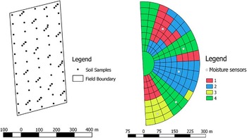
A Management Zones (MZs) approach was applied to schedule VRI. Soil parameters and NDVI vegetation indices by LANDSAT images were integrated to delineate the MZs. Soil was sampled in 103 points following a mixed-sampling scheme (Chiericati et al., Reference Chiericati, Morari, Sartori, Ortiz, Perry and Vellidis2007), collecting 55 samples at the nodes of a 55 m x 65 m grid and 48 additional points at the nodes of 16 transects at 2.5, 15 and, 30 metres from the grid node (Fig. 1). Soil samples were then analysed for texture (Mastersizer 2000, Malvern Instruments Ltd., Great Malvern, UK) and spatially interpolated by ordinary kriging. Maize vigour spatial variability at the peak of previous growing seasons (29 June 2009 and 24 June 2013) was estimated by NDVI maps using LANDSAT 7 satellite images. In spite of the low spatial resolution, LANDSAT 7 images were used since they were freely available and have the same spatial resolution of the VRI centre pivot (30 m). MZs were identified using Management Zone Analyst 1.0 (Fridgen et al., Reference Fridgen, Kithcen, Sudduth, Drummond, Wiebold and Fraisse2004), which subdivide the area in clusters (corresponding to the MZs) through a unsupervised fuzzy c-means clustering method. The number of clusters was evaluated with the Fuzziness Performance Index (Fridgen et al., Reference Fridgen, Kithcen, Sudduth, Drummond, Wiebold and Fraisse2004).
Soil samples points and Pivot VRI management zones, soil moisture sensors position. Zones 1 to 3 corresponds to VRI MZs, Zone 4 corresponds to areas irrigated uniformly (non-VRI).

Three MZs were delineated under the area of the pivot (Zones 1–3) on the VRI map shown in Figure 1. Three areas in which irrigation would be applied uniformly were superimposed on the field. These areas are indicated as Zone 4 in Figure 1.
Variable rate irrigation system assessment
The centre pivot was coupled with a variable zone control system provided by Valley® Irrigation. Each sprinkler was controlled (ON or OFF) by pneumatically-actuated flow-control valve that was normally-open (Dukes et al., Reference Dukes and Perry2006). The 96 pivot sprinklers were grouped into 10 control zones (about 25 meters length) with 8 sprinklers each one. The distribution uniformity test was measured three times before the irrigation season according to the ASABE standards (ASABE, 2001) and the testing layout proposed by Dukes et al. (Reference Dukes and Perry2006).
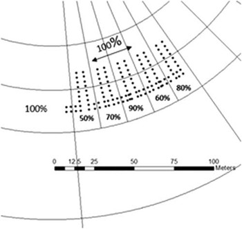
The water distribution uniformity of the conventionally operated pivot (without VRI) calculated with the low quarter Distribution Uniformity (DUlq) (Burt et al., Reference Burt, Clemmens, Strelkoff, Solomon, Bliesner, Hardy, Howell and Eisenhauer1997) and the Heermann and Hein coefficient of uniformity, showed optimal performances, with a DUlq of 0.91 and CUH of 93.9. In order to test the VRI performance, the prescribed irrigation application rate (predicted) was compared with the observed application rate (observed) (O’Shaughnessy et al. (Reference O’Shaughnessy, Urrego, Evett and Colaizzi2013). The variable rate application was set to 50%, 60%, 70%, 80% and 90% of the maximum pivot application rate (30 mm depth). The catch cans were placed into two patterns, transect and arc-wise (Fig. 2) within the third span of the pivot. The depth data from the catch cans were then converted into percentages and fitted to a calibration linear model between predicted and observed application rates. Root mean square error (RMSE) and determination coefficient (R2) highlighted a good fit between predicted and observed measurements variable rate application sector (R2=0.86 RMSE=1.7).
Catch cans testing layout, where points are cans and lines define variable rate application zones.

Variable Rate Dynamic prescription
Soil water content information (soil moisture sensor) was used to schedule the variable irrigation volumes. In each MZ, a soil water monitoring station consisting of a EM50G wireless cellular data logger and an array of three 5TE sensors (Decagon Devices Inc., Pullman, WA, USA) was installed. Sensors were first calibrated in laboratory (accuracy of ±4%) and then set along the soil profile at 10, 30 and 50 cm depth. The profile was then characterized by soil texture and bulk density (ρb) (core method) in order to calculate the water balance (Topp et al., Reference Topp, Davis and Annan1980).
Crop monitoring and Irrigation Water Use Efficiency
Maize biomass was collected on three different dates (72, 102 and 115 Days After Planting – DAP) from near the soil sensor network points stations in order to monitor crop response to water management.
At the same time maize vigour was monitored by NDVI maps created from Unmanned Aerial Vehicle (UAV) and satellite (SENTINEL-2 and LANDSAT 8) images. SENTINEL-2 data are acquired in thirteen spectral bands in the visible, VNIR and SWIR ranges with spatial resolution varying between 10 m and 60 m depending on the spectral band. Landsat 8 Operational Land Imager (OLI) images consist of nine spectral bands with a spatial resolution of 30 m.
The UAV used in this study was a fixed wing eBee (Sensefly®/ Menci) fixed wing equipped with multiSPEC 4 C that reads in the green (550 nm), Red (660 nm), Red edge (735 nm) and NIR (790 nm) wavebands.
Yield data were recorded, by a NewHollandTX64 combine harvester equipped with a yield monitor system (grain mass flow and moisture sensors). The SMS software version 3.0TM (AgLeader Technology, Inc.) was used to read the row yield data (expressed at 14% dry matter). Raw data were cleaned for the field-edge effects or low data due to a harvester manoeuvres. Irrigation water use efficiency was calculated comparing irrigated yield with an unirrigated regime in relation to the water volume (Howell et al., Reference Howell2003):
 $$IWUE\,{\equals}\,{{\left( {Y_{{gi}} \,{\minus}\,Y_{{gd}} } \right)} \over {IRR_{i} }}$$
where, IWUE is the irrigation water use efficiency (kg m–3), Ygi is the economic yield (kg ha–1), Ygd is the rainfed yield (crop yield without irrigation) and IRRi is the irrigation water applied (m3 ha–1).
Results and discussion
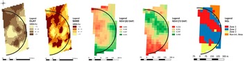
The soil texture maps showed a variability and distribution similar to the NDVI maps (Fig. 3). Soil texture shows a high spatial variability with a coefficient of variation (CV) of 25% and 23% for sand and clay respectively. The field present a marked variability on the north-south axis, with a higher content of sand on the southern part and clay areas toward north.
Thematic maps: clay, sand, NDVI 2009 (82 DAP), NDVI 2013 (72 DAP) and MZs.

Cluster analysis identified four MZs (Fig. 3). Only 3 of them were retained because the fourth area corresponded to the non-irrigated areas on the corners of the field. Zone 1, located in the north eastern portion of the field, was characterized by silty loam texture, Zone 2, in the central area of the field, by loam texture and Zone 3, in the south-western part, by sandy-loam texture. NDVI values were strongly dependent on the season and the management zone, with zone 3 presenting the highest value in a rainy year (2009) and the lowest in 2013, year characterised by a prolonged drought. In both cases the uniform management of irrigation was not able to optimize the vegetative vigour of the crop (Fig. 3).
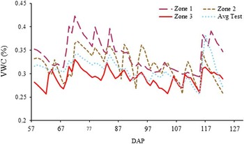
The irrigation season of 2015 was characterized by very high temperatures and low rainfall (two small rainfall events in July and August). In the three VRI MZs, irrigation was scheduled when VWC approached 35%, 32% and 28.5% respectively for MZs 1, 2 and 3. In the Uniform MZ, irrigation was scheduled at each passage of the pivot at the maximum rainfall rate considered (38 mm). The reference evapotranspiration (ET0) was high with daily peak values close to 6 mm day–1 leading to a high water demand in the critical grain filling growth stage.
From mid-July (93 DAP), the water demand resulted so high that the limiting factor became the time required by the pivot for completing a rotation. This caused a progressive decrease of the VWC with a return to Field Capacity only at the beginning of August after a rainfall event (Fig. 4).
Volumetric Water Content (VWC) data in all MZs.

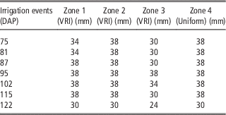
Despite of this, compared to conventional irrigation management, based on the water balance of the loam zone, VRI allowed a 40 mm water saving in the Zone 3 (sandy-loam) and 8 mm in the Zone 1 (Table 1).
Irrigation prescription per zone during irrigation season (38 mm is the maximum application rate allowed by the pivot).

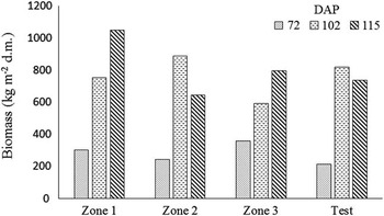
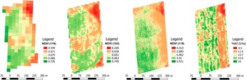
Within the 3 sampling dates, maize biomass did not present significant differences between zones (Fig. 5). It is anyway evident a marked variability, partly due to lodging, which was particularly evident in MZ 2. NDVI measurements (Fig. 6) confirm the reduced crop vigor in MZ 2, particularly with Sentinel-2 and UAV images, and show a good development in MZ 3 (south-western area), despite the coarse texture of this part of the field. This result is particularly interesting considering the prolonged drought of summer 2015.
Biomass monitoring per zones.

Monitoring NDVI thematic maps: LANDSAT 8 (DAP 119), SENTINEL-2 (DAP 123) and UAV (DAP 115) and grain Yield map (grain humidity 14%).

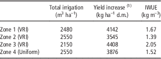
In Zone 1, water application rate and yield almost close to the zone irrigated uniformly (–3% and +7% respectively) (Table 2). The irrigation management of zone 2 was the same as for the uniform zone, but yields were slightly lower (–9%). In Zone 3 the VRI allowed a reduction of the volume applied (–16%), together with a yield increase of +14%. Considering the whole field, however, maize yield did not show any significant differences between VRI and uniform zone (field average of 12.5 t ha–1 at 14% moisture content), while overall IWUE was 12% higher than the uniform zone. Compared to the uniform zone, IWUE for the VRI zones were: Zone 3 (+35%), Zone 1 (+10%), and Zone 2 IWUE (–9%).
Total irrigation amount, average maize yield increase observed in 2015 and IWUE.

(1) Yield increase (kg ha–1 d.m.) compared to non-irrigated test
Conclusions
The VRI system gave interesting operational results despite an unfavorable meteorological pattern. The summer of 2015 was indeed characterised by exceptionally high temperatures and by a prolonged drought, starting before maize flowering to mid-August. These conditions did not allow us to exploit the full potential of VRI, maximizing irrigation demand regardless of the water retention potential of soils. Nevertheless, the VRI optimized the irrigation intake, maximizing yields due to soil moisture monitoring stations, allowing a fine tuning of the irrigation, particularly in MZ 1 and 3. In turn, the maize yield did not show any significant differences among the zones, while water savings compared to the business-as-usual regime ranged from 8 mm (low irrigation requirement zone) to 40 mm (high irrigation requirement zone). In particular, it is worth pointing out the results obtained in the ‘‘sandy’’ area (Zone 3), where it was possible to obtain a reduction of the water applied, still maintain vegetative indexes and a yield not different from the irrigated check. Even if the results should be confirmed in seasons with different meteorological patterns, Variable Rate Irrigation (VRI) systems, integrated with sensor technologies, seems then to represent an advance in irrigation, addressing the complex spatial and temporal interactions observed in the field and their effects on the crop water requirements.