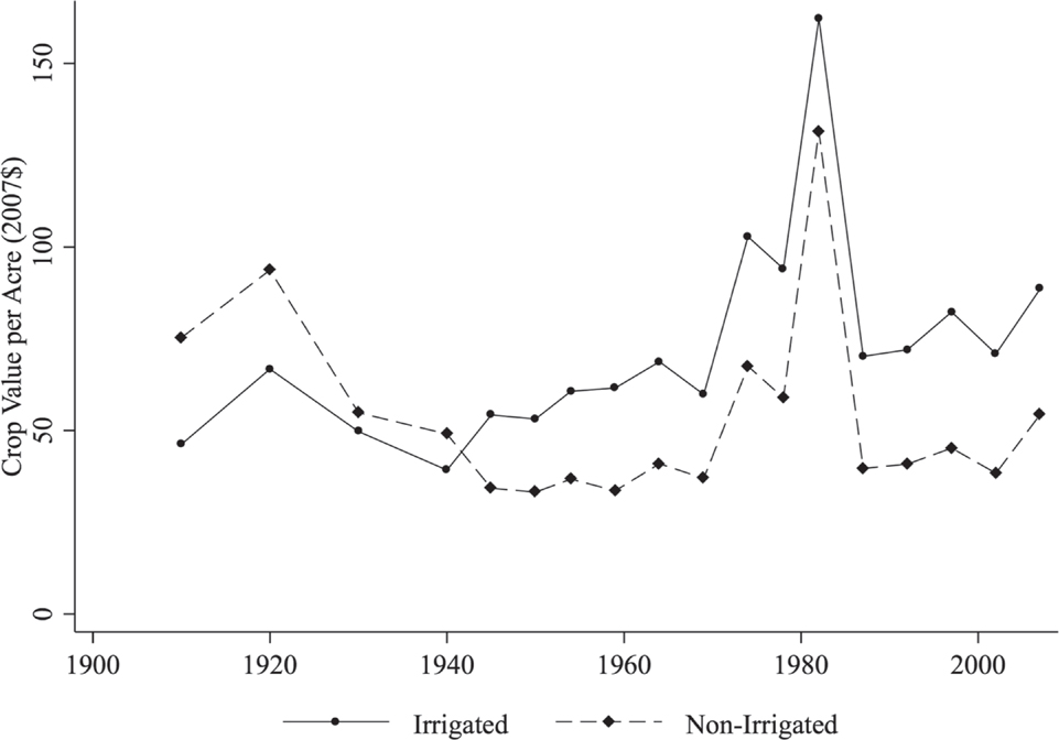
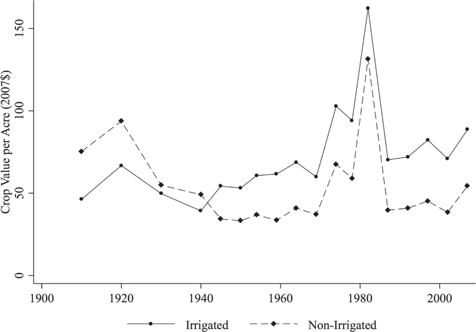
Starting in the late 1930s, agriculture in the United States underwent a productivity revolution. Crop output per acre was stagnant from 1900 through 1935, but then increased at an average of 2.1 percent per year for the next 60 years (Gardner Reference Gardner2002, p. 22). Many explanations have been offered for the production shift, including modernization of equipment and chemicals (Rasmussen Reference Rasmussen1962), regulatory changes (Clarke Reference Clarke1994), and the electrification of farms (Lewis and Severnini Reference Lewis and Severnini2018; Kitchens and Fishback Reference Kitchens and Fishback2015). This article examines the importance of irrigation in the marked increase in farm productivity during this time period. As shown in Figure 1, areas of the United States that employ irrigation water began producing more crops per acre, measured by market value, soon after 1940. In 2012, although only 28 percent of harvested cropland was irrigated, it provided nearly half of the total value of crop sales, suggesting an important role in overall agriculture productivity (USDA 2018).
Average Crop Production per County Acre by Census Year Bifurcated by the Presence of Irrigation
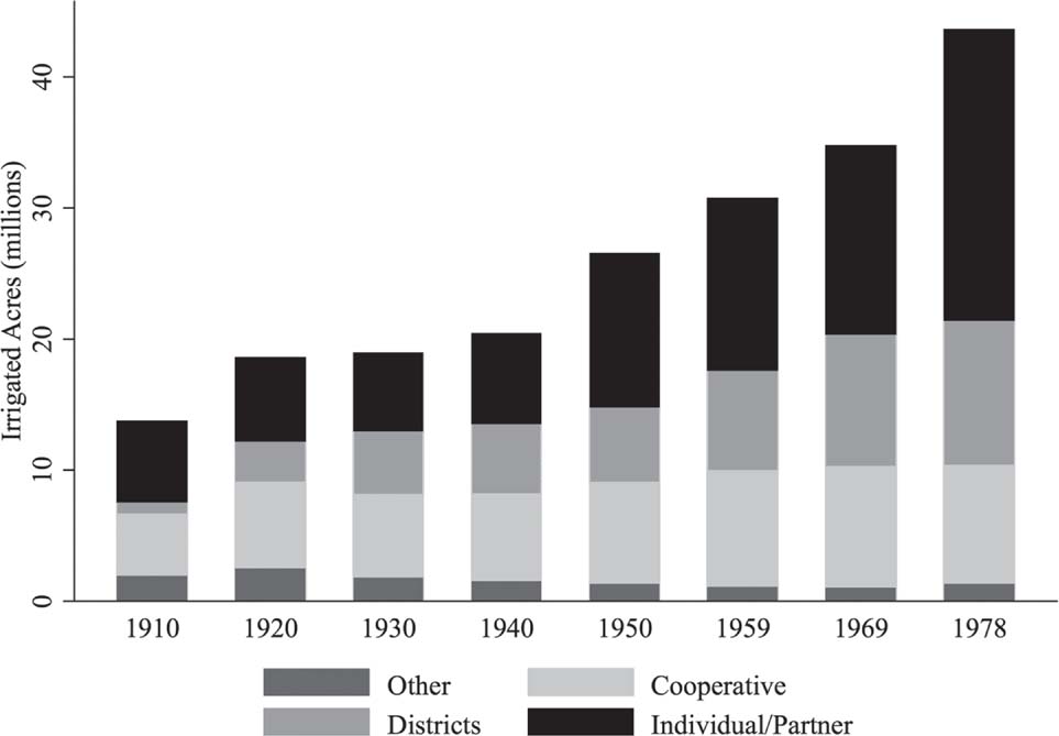
Notably, irrigated acreage in the United States, like productivity, remained relatively stagnant during the early twentieth century. From 1910 to 1940, total acreage irrigated hovered around 20 million acres, almost all of which was privately developed in the arid western territory of the United States. In Figure 2 we show the total irrigated acreage by census year for the 17 western states. It is after 1940 that irrigated acreage grows, doubling by 1978, before stagnating in the West yet again while adoption of irrigation continues in the East.Footnote 1 This additional irrigation, while increasing crop production, was costly due to investment in irrigation works and energy to move water. We propose to explore the benefits and, to a lesser degree, the cost of expanded irrigation in the United States post-1940, focusing on the arid area west of the 98th Meridian.
Total Irrigated Acres in the Western States by Irrigation Enterprise Organization

The growth in irrigated acres after 1940 occurred because of increases in ground and surface water availability due to changes in institutions and technology. Stephen Bretsen and Peter Hill (Reference Bretsen and Hill2006) attribute the growth to irrigation districts and their ability to reduce the transaction costs in financing shared infrastructure. Irrigation districts, along with the federal support from the U.S. Bureau of Reclamation (BOR), came about at the turn of the twentieth century, but the growth in irrigated acres did not come until after the 1940s. This aligns with the big dam-era driven by the confluence of engineering breakthroughs, New Deal policies, and growing demand for (hydro-)electricity (Billington and Jackson Reference Billington and Jackson2006). Beginning with the Hoover Dam’s completion in 1936, federal surface water storage grew from negligible amounts to more than 40 million acre-feet by 1978. However, this is only half the story. Shown in Figure 2, irrigated acreage expanded even more under the “individual/partnership” enterprise type from 1940 to 1978. Though smattered with small surface water enterprises, this category grew primarily due to individuals expanding groundwater use. Following rural electrification (1935–1955) and the advent of the center pivot in 1948, use of groundwater beneath farms became economical and profitable in more of the United States. Our approach is to measure the impact of the technological and regulatory changes that led to well development and large reservoir construction after 1940. While many counties had some irrigation starting as early as the mid-1800s, we examine the gains beyond these small irrigation works, afforded by the breakthroughs that occurred around 1940.
We examine how access to additional irrigation water broadly affected the development of agriculture in the western United States and separate the effect attributable to surface water storage from that of groundwater development as well as the effect of having access to both types of water. While surface water and groundwater development have been studied in isolation, they have not been examined simultaneously. We expect differences due to the distinct issues that confront surface diverters and groundwater pumpers as well as the institutions, such as property rights, that have separately evolved to address these differences. Surface water storage requires immense capital; groundwater storage is free. Surface water requires cooperation with neighbors to deliver and divide the water, though the water itself is generally cheap or even free. Groundwater users require no upfront cooperation and can develop the source independently, though they face costs in pumping the water. Surface water availability is uncertain year-to-year owing to climactic conditions, whereas groundwater users are able to extract water independent of climactic and institutional limitations. However, groundwater users may face challenges due to common-pool resource properties and the non-renewable character of some aquifer systems.
To quantify and test the impact of the alternative sources of new irrigation water, we use data from the U.S. agricultural census to track measures of irrigation adoption along with crop income and land values, primarily from 1910 to 2007. While the pre-1910 period sees growth in irrigation across the West, the period from 1910–1940 is relatively stable with little additional irrigation development. For this reason, we use the level of irrigation developed up to 1910 as the baseline in setting up our analysis of the effect of the technological and regulatory changes that expanded irrigation around 1940. To identify the effect of irrigation, we compare counties before and after 1940 based on their potential access to surface water storage projects and groundwater, defined only by physical characteristics to address concerns of endogeneity between reservoir construction, well development, and agriculture outcomes. Although there is some minor development prior to 1940, the time period and physical measures predict irrigation development quite well.
Results indicate that areas with groundwater access experienced the largest irrigation, crop production, and farm value gains after 1940. In contrast, access to augmented surface water supplies through large dam construction netted smaller gains in irrigated acreage, crop production, and farm value, though gains in production are capitalized into land values more efficiently. The results are more nuanced and somewhat surprising for areas that have access to both large streams and groundwater. These regions experience very little growth in land value post-1940 because they already enjoyed a significant premium prior to 1940, likely because they already benefitted from groundwater springs.
After 1940, we estimate that areas with better access to groundwater, large streams, or both for irrigation increased crop production by $19 billion annually relative to western areas with only small streams. This is large, equivalent to 90 percent, relative to the total growth after 1940. This gain is inclusive of other components of the agriculture revolution and some relocation of agriculture from small-stream areas (and to a greater extent from the eastern United States). From a policy perspective, our results suggest that irrigation was only a partial substitute for precipitation; where low-cost surface irrigation development had already occurred, the marginal benefit of groundwater irrigation was larger than the marginal benefit of the creation of large surface water projects.
Background and Literature
With a few exceptions, precipitation in the United States west of the 98th Meridian is not sufficient for intensive agricultural production. While the ability of the region to support agriculture was questioned initially, early settlement in areas with access to water demonstrated that agricultural production was possible. American Indians were the first irrigators, and early Spanish settlers in New Mexico and Mormons in Utah organized development around irrigation works. Water governance institutions evolved concurrently with the development of surface water sources. Western states have generally adopted the prior appropriation doctrine, or “first in time, first in right” (Clark Reference Clark1960; Anderson and Hill Reference Anderson and Hill1975; Burness and Quirk Reference Burness and Quirk1979; Gisser Reference Gisser1983). Users acquire a right to use water by diverting it from a stream and putting it to beneficial use as defined by state law. In a given year, these appropriators receive water based on the date of their first diversion. Senior appropriators are thus guaranteed access to irrigation water, securing the key input necessary for agricultural production. Though the unequal division of risk may create some inefficiency in surface water division today (Burness and Quirk Reference Burness and Quirk1979), the system protected, and thus incentivized, early investment in diversion ditches. This system of property rights also had efficiency advantages by allowing for later appropriators to learn about the size and reliability of a stream from early appropriators (Leonard and Libecap Reference Leonard and Libecap2016). Other local collective water management systems were also used effectively to secure water for irrigation, for instance, in the New Mexican acequias (Smith Reference Smith2016).
At the turn of the twentieth century irrigation was already making an economic impact; while the average dryland farm sold for $1.25/acre (1907 $), irrigated land fetched up to $300/acre in Colorado, $700/acre in Washington, and $1,800/acre in California (Taylor Reference Taylor1907). However, the potential for irrigated agriculture in the West was constrained, with the supply of irrigable land “very great” compared to the amount of available irrigation water (Taylor Reference Taylor1907). The first settlers selected land that required minimal investment to irrigate (Whitbeck Reference Whitbeck1919, p. 223), but land in locations favorable to receiving water from small irrigation works was limited, and most of this land had been put into irrigation by the turn of the century. “As the opportunities for irrigation through easy and inexpensive methods of diversion of water gradually disappeared there came a need for larger enterprises and higher per-acre expenditures to develop them” (Hutchins, Lewis, and Ewing Reference Hutchins, Lewis and Ewing1938, p. 694). Longer ditches may have been needed, but proponents of development argued “that the regulation of the flow of Western rivers is almost as important as the building of canals to divert their waters,” citing the uselessness of excess flood water in the spring and empty canals in the late summer (Mead Reference Mead1910, p. 355).
Irrigation collectives and individual appropriators organized around ditches struggled to raise the necessary capital to increase irrigation works beyond small diversion dams (Bretsen and Hill Reference Bretsen and Hill2006). The expensive development of reservoirs presented a financial problem: “Their construction has been conclusively shown to be an undertaking too vast for private effort,” argued President Theodore Roosevelt, and “[t]he Government should construct and maintain these reservoirs as it does other public works” (quoted in Teele Reference Teele1902, p. 395). In 1902 the passage of the Reclamation Act brought the U.S. government into the water delivery business.
Despite federal encouragement, irrigated acres in the West stagnated from 1920 to 1940. In questioning whether western irrigation had been a success, Ray Whitbeck claimed “the answer is neither Yes nor No” (1919, p. 230). He pointed to the 55,000 non-federal, mostly “small individual or partnership undertakings (p. 223)” that mostly succeeded, but also indicated that the BOR projects to date were largely vacant as settlers were reluctant to take on the added expense of repayment. Donald Pisani (Reference Pisani2002, p. 293) in providing a historical perspective concludes, “the accomplishments of federal reclamation from 1902–1935 were modest.” This changed after 1940 with the addition of new water supplies, both surface and ground, that increased irrigated acres from around 21 million in 1940 to more than 43 million by 1978.
It was the large public works projects initiated by the federal government during the Great Depression that brought additional surface water storage and delivery projects into operation (Cochrane Reference Cochrane1979, p. 225). Advances in dam engineering, movement towards multi-purpose dams (hydro-electricity), New Deal projects, and basin level planning paved the way for the federal government to construct numerous dams (Billington and Jackson Reference Billington and Jackson2006). The first major BOR reservoir project, and still its largest, was the Hoover Dam, which began operating in 1936. The zest for building persisted as the Army Corp of Engineers and the BOR vied for public projects supported by western politicians (Reisner Reference Reisner1993). While the literature on the financial returns of the BOR projects has generally been critical of the public investments (Reisner Reference Reisner1993; Shapiro Reference Shapiro1973), there has been little work to put the impact on agricultural productivity in context.
In terms of groundwater, some development had occurred as early as 1900, but this activity was primarily limited to California (Smith Reference Smith1915, p. 374; Bowman Reference Bowman1911, p. 16). The amount of acreage directly irrigated was still quite small in the early twentieth century. This began to change after a series of droughts in the 1930s (Hutchins, Lewis, and Ewing Reference Hutchins, Lewis and Ewing1938). However, extensive groundwater development did not begin until after WWII, aided by improved access to electricity, combustion engines, deep well turbine pumps and right-angle drives, and the invention of center pivot irrigation, which allowed for more reliable delivery of groundwater to crops via sprinklers (Lewis and Severnini Reference Lewis and Severnini2018; Hornbeck and Keskin Reference Hornbeck and Keskin2014; Heermann Reference Heermann2003). Indirect use of aquifers by irrigators, whether knowingly or not, could have occurred even prior to development where ground and surface water systems are linked, usually along larger streams. In periods of low surface water flow, groundwater springs act to supplement streams in a process called baseflow.
While not a precisely defined date, we use the level of irrigation developed via small surface irrigation works, on small and large streams alike, up to 1910 and through 1940 as the baseline and analyze the effect of the technological and regulatory changes that expanded ground and surface water irrigation after the period of stagnation. A similar approach was used in analysis of the abrupt increase in the value of the Ogallala aquifer with the rapid adoption of irrigation after 1940 (Hornbeck and Keskin Reference Hornbeck and Keskin2014, Reference Hornbeck and Keskin2015). The key challenge with estimating the causal impact of a water resource on agricultural production is the potential for aquifers to be co-located with other land characteristics favorable to production. To overcome this, these articles exploit the variation in aquifer access using a pre/post design, where initially aquifer access does not provide irrigation benefits through direct development.
Separately, analyses have been performed on surface water and dam construction, although not for the entirety of the western United States (e.g., Hansen, Libecap, and Lowe Reference Hansen, Libecap and Lowe2011). A major challenge with finding a causal relationship between the placement of infrastructure and economic outcomes is the selection of infrastructure sites for factors that also increase farm productivity. One solution is to use an instrument for the location of dams, for example, stream gradient (Duflo and Pande Reference Duflo and Pande2007; Lipscomb, Mobarak, and Barham Reference Lipscomb, Mobarak and Barham2013). Another potentially confounding issue is that dams provide electrical power and irrigation water. However, by around 1950 with the implementation of high-capacity electricity transmission, the benefits of electricity were spread over larger areas, and there is little difference in electricity availability in counties with and without dams after this time (Severnini Reference Severnini2014).Footnote 2 In contrast, even as large dams were built in the late 1930s and 1940s, the water delivery infrastructure took longer to be completed. For instance, construction on the Central Valley Project started in 1937, but the first irrigation water was not delivered in California until 1951 (Wahl Reference Wahl1989, p. 50).Footnote 3
The overall impact of the availability of new water supplies for irrigation post-1940 has been underappreciated in the literature. Prior to the developments discussed in this article, there was extensive discussion in the top economics journals of the critical issue of irrigation in the western United States (e.g., Taylor Reference Taylor1907; Coman Reference Coman1911; Hess Reference Hess1912; Coulter Reference Coulter1912). However, literature on agricultural development since the early 1900s has generally ignored evaluating the impact of irrigation. Karina Schoengold and David Zilberman (Reference Schoengold and Zilberman2007), in providing a summary of the economics of irrigation and development, simply state that irrigation has been a significant factor in increasing yields. Yet many of the works examining the U.S. agricultural productivity revolution do not mention irrigation. For instance, Yair Mundlak (Reference Mundlak2005) reviews the literature on the growth of U.S. agriculture and mentions irrigation only in the context of Asian rice production. Sally Clarke (Reference Clarke1994) suggests the productivity revolution was a result of regulatory policies, but she does not address the multitude of regulatory and governmental interventions to provide water to western farmers. Wayne Rasmussen (Reference Rasmussen1962) provided one of the early assessments of the impact of technological change in productivity gains, yet failed to discuss technological advances in center-pivot irrigation wells and water storage and delivery technology. Carl Kitchens and Price Fishback (Reference Kitchens and Fishback2015) show the large impact rural electrification had on the increase in farm output, productivity, and land value, but do not discuss irrigation as a potential intermediary step. Although the role of irrigation has not been missed entirely—Joshua Lewis and Edson Severnini (Reference Lewis and Severnini2018) show the close relationship between the rollout of the U.S. electrical grid and the development of irrigation, which on-farm electricity made more cost-effective—the causal effect of irrigation on agricultural development has not been fully explored.
Our analysis closely mirrors the work of Richard Hornbeck and Pinar Keskin (Reference Hornbeck and Keskin2014) on the Ogallala Aquifer. They find that aquifer access resulted in a $25 billion increase in value relative to farms near, but without access. We differentiate our work from theirs and other related studies in three ways: (1) by expanding the scope of the study to cover the entire western United States; (2) by including surface water development in the analysis; and (3) by examining in detail the trends in irrigation and irrigation organizations throughout the study period.
Data
For our analysis, we construct a panel data set consisting of 2,920 U.S. counties with 18 observations from 1910 to 2007. Our main analysis, however, uses only the subsample from the arid 17 western states. To address the climactic gradient of the Great Plains, we keep only counties west of the 98th meridian, an approximation of the transition from the sub-humid to semi-arid portion of the United States, leaving 684 counties in our primary data set.
We use data from the agricultural census to look at total value (land value plus value of buildings), crop production (combined value of all crops produced), and irrigated acreage from 1910–2007 across 18 distinct censuses.Footnote 4 The monetary measures are adjusted to constant 2007 dollars for inflation using a CPI index. These are scaled by county area to adjust for variation of county sizes. In addition to these outcomes, we also consider structural variables such as the number of farms, total farm acreage, and the average size of farms. These economic data are digitized by Michael Haines (Reference Haines2010).
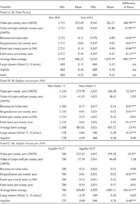
Because our economic data span a significant portion of the twentieth century, we adopt 1910 counties as our observations, reweighting data from other years to fit these borders (Minnesota Population Center 2006).Footnote 5 For the process to yield accurate aggregations in all cases, the census farming data would need to be uniformly distributed over space. Though this is unlikely on the whole, most instances are of a single county being divided into two counties in which case the aggregation is accurate independent of the spatial distribution of farms and irrigation. Furthermore, county borders are relatively stable from 1910 onward.Footnote 6 The resulting variables, and others, introduced later, are fully described in the Online Appendix Table A1 and descriptive statistics are provided in Table 1.
Descriptive Statistics by Period and Water Access

*** p < 0.01
** p < 0.05
* p < 0.1
a For purposes of comparison in Panels B and C, fraction of the county overlaying both the large stream buffer and an aquifer is not distinguished
Source: See data section in text.
Our research question focuses on the agricultural impacts of developing groundwater wells and surface reservoir construction. Though we have some data on the number of wells in each county from the agriculture census and we collect data for location and size of dams from the National Inventory of Dams (USGS 2006), for reasons explained later, our empirical strategy relies on more general measures of potential access. For our measure of expanded surface water, we extract stream segment locations from the USGS (2014). The streams are ranked using Strahler Order, an algorithm-based measure that generally gets larger as tributaries meet. The scale goes from 1 (the smallest streams) up to 7 (largest streams).Footnote 7 Because larger streams with more tributaries are better suited for reservoir construction, we build our measure from stream segments of order 4–7. We create a 15-mile buffer on each side of the large streams and then calculate the fraction of each county that is overlaid by one of these buffers. We define this as the area that could potentially receive water from a large reservoir. We further distinguish by any portion that overlaps with aquifer access, defined later. We also calculate 5, 10, 20, and 25-mile buffers for robustness checks, but the 15-mile buffer is preferred as this meshes well with observed conveyance. In 1910, the average irrigation ditch was only 1.9 miles and in 1930 the average had actually decreased to 1.4 miles. Even by 1969, the median enterprise still had less than 4 miles of ditches, though some longer ditches brought the average up to 13 miles.Footnote 8 All told, we find the 15-mile buffer appropriate, as even the larger conveyance structures are seldom perpendicular to stream, so distance from stream is less than the miles travelled, though exceptions do exist.
Groundwater access is more straightforward to define. We draw on the physical presence of an underlying aquifer as located by the U.S. Geological Survey (USGS 2003). As we did with the stream buffer, we calculate the fraction of each county that overlays an aquifer to define the extent of its groundwater access. Because groundwater is typically used in close proximity to the source, we do not construct any buffer. Last, we combine both the surface buffer and aquifer layers in GIS and compute the fraction of each county that has overlapping access to both groundwater and large streams. On average, 15 percent of each county has access to only surface water, 36 percent to only groundwater, and 22 percent enjoy joint access. Notably, while there is significant overlap between the two sources of water, the statistical correlation between the two independent measures is nearly zero (0.0101). While our main analysis does not differentiate between types of aquifer, we do include a measure of heterogeneity, well yield, in some of the alternative specifications. Well-yield data is constructed for the major aquifers in the United States using USGS and state agency sources.
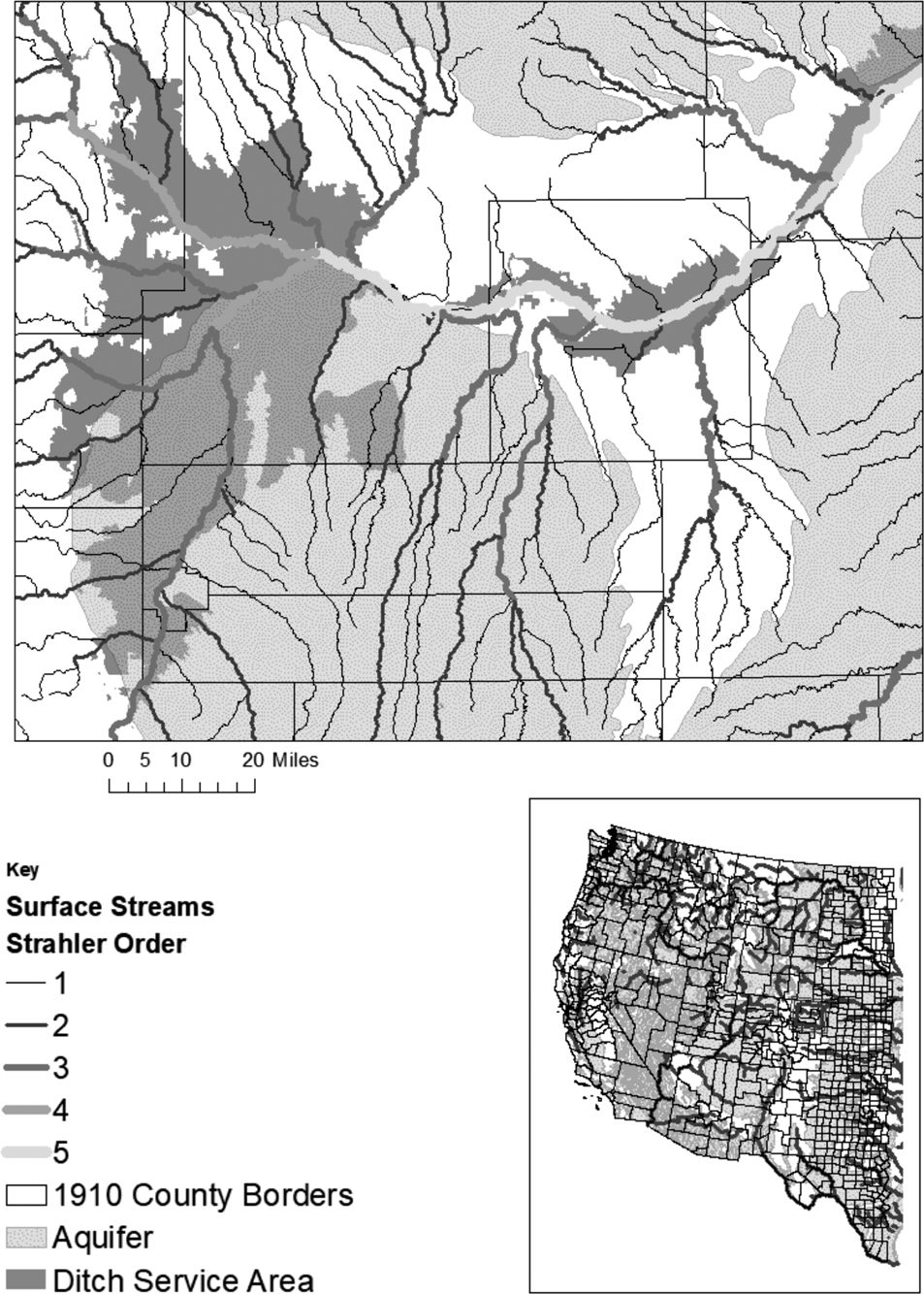
To illustrate our method of constructing the stream and aquifer data, Figure 3 provides an overview of the west and a detailed close-up of the underlying physical variables in northern Colorado. For a more thorough overview, see Figures A1–A3 in the Online Appendix, which show the raw and constructed data. The construction of the Strahler Order can be seen as stems come together on the close-up map. Based on the extent of land irrigated by surface ditches, it is clear that a lot of land can be serviced by smaller streams, though as we demonstrate later, very little storage occurs on these smaller streams. The figure demonstrates that lands irrigated by surface water tend to be close to streams, certainly within the 15-mile buffer. It also shows that access to aquifers may or may not coincide with surface irrigation, underscoring the potential need to further distinguish areas that have access to both.
Water Access and Irrigation in Western United States

In addition, we gather a number of fixed variables that likely influence agriculture production and value: longitude and latitude, elevation, soil quality, and mean and range slope. To account for variation in precipitation that would impact irrigation adoption and agricultural economic outcomes, we use historical data from PRISM (2004) to calculate average precipitation for each county based on annual precipitation from 1900–1980. Last, we also include population measures to account for relative land scarcity that may push up land value independent of its agricultural productivity. However, in recognition that population may flourish in areas that are agriculturally more productive—introducing endogeneity—we opt to use 1910 population numbers, making it plausibly exogenous from later irrigation development.Footnote 9
Given the spatial and temporal span of our data set, overall means conceal significant variation. Accordingly, Table 1 provides the means for subsamples based on time, surface access, and groundwater access. As expected, there are large gains in land value and production across time as seen in Panel A. Pre-1945 distinctions across levels of large stream and groundwater access, Panels B and C, are much smaller, though statistically significant in some cases. Additionally, differences across the three regions in the economic outcomes are significant while water access measures are more similar (summary provided in Table A2 of the Online Appendix), indicating important insight can be gained by examining the regions individually as well as in aggregate.Footnote 10
Empirical Model
To explore the differential influence of groundwater and expanded surface water access, we would like to run the following regression:
 $\log ({{\rm{Y}}_{{\rm{it}}}}) = \alpha + f({{\rm{S}}_{it}};{{\rm{G}}_{it}};\mathbf{\beta} ) + g({\mathbf{C}_\mathbf{\var{i}}},{\mathbf{T}_\mathbf{\var{t}};\mathbf{\theta} ) + {{\rm{u}}_{{\rm{it}}}},$
where Yit is the (per acre) value of farmland in county i in year t. As laid out, we expect this to be a function of access to surface water storage (S it ) and the number of wells drawing on groundwater sources (G it ), including possible interactions between the two sources of water. In addition, value is impacted by a number of other attributes, both observed and unobserved, that vary by county ( Ci – precipitation, soil quality, latitude, elevation, population, access to markets, etc.), and that vary only by year (T t – crop prices, technology, financial markets, etc.).
Empirical estimation of the equation is difficult for two reasons. First, the location of wells and reservoirs are unlikely to be random in space or time. Second, there are significant data availability issues. For instance, after the 1950 census there is no longer information reported on the number of wells drawing groundwater. Similarly, data on the number of acres irrigated with the BOR water at the county level are only available in 1910, when very little was irrigated by the organization, and in 1950. Besides the limited availability, using irrigated acreage to define access is itself problematic since irrigators can choose to apply more water to existing acreage or expand acreage. And while we could construct treatment by the presence of a BOR dam and reservoir, these projects can, and often do, provide water to land in counties downstream.Footnote 11
To overcome both issues, we draw on an instrumental variables-type approach, using physical measures of potential access as well as a break in time that greatly increased the odds of development of both sources. Because the data for our endogenous variables, well and surface water storage access, are incomplete, we cannot directly utilize the two-stage IV approach. To overcome this issue, we first examine what we can say about the relationship between physical measures of access and dam and well construction. Then, we turn our focus to the reduced form in the Results section. In particular, we conduct a difference-in-differences type analysis with three distinct types of treatment captured by the various water access measures: percentage of land within the large stream buffer, percentage overlying an aquifer, and percentage with joint access. Because our physical access measures are continuous, we are able to draw on this additional variation for identification and our estimates do not solely rely on counties with low access (as we have defined it) but also compare counties with relatively more or less access to identify the impact. Our approach is similar to an intent-to-treat strategy on aquifer and large stream access, but with some counties getting put into the wrong treatment category. This is the case because in order to get an exogenous measure of water access for every U.S. county, we necessarily observe access imprecisely. For instance, a county over an aquifer too deep to extract or next to a river in a deep canyon too expensive to pump from. Alternatively, those politically connected could lobby for long-distance diversion bringing surface water to an area beyond our physical measure.Footnote 12
With static measures of treatment, we are precluded from using actual time of development within a county as the time of treatment. Instead, we define a pre- and post-treatment period sometime between the 1940 and 1945 censuses. Although some BOR Projects and other efforts had taken place by this time, large reservoir infrastructure took off after this point. Likewise, some groundwater sources had been limitedly developed, but post-1940 technological improvements and expanded access to cheaper energy greatly increased the pumping from aquifers. By assigning a uniform treatment period, concerns over endogenous timing are also removed, as we again rely on the potential for treatment rather than actual treatment as our identification strategy.
Defining the indicator variable
 $I_t^P$
such that
 $I_t^P = 1$
when t > 1940, the main regression to identify the impact of reservoirs and groundwater is
 $\log ({\rm{Y}}_{\rm{it}}) = \sigma \cdot {\rm{I}}_t^P{S_i} + {\rm{\rho}} \cdot {\rm{I}}_t^P{{\rm{A}}_i} + \phi \cdot {\rm{I}}_t^P{{\rm{J}}_i} + \varphi \cdot {S_i} + \alpha \cdot {{\rm{A}}_i} + \eta \cdot {\rm{J}}{ _i} + {{\mathbf{\Psi}} _t} \cdot {{\mathbf{C}}_i} + {\gamma _i} + {\tau _t} + {{\rm{u}}_{{\rm{it}}}}.$
Si, Ai , and Ji are the variables of interest, capturing the exclusively defined fractions of the county with access to large streams, groundwater, and joint access, respectively.Footnote 13 The coefficient σ estimates the differential increase for counties with access to large streams after 1940; ρ is the increase in the relationship between land value and proportion over aquifer after 1940 for low surface water counties; and ϕ is the increase in the relationship between land value and proportion over the aquifer and the high surface water buffer after 1940. Our identifying assumption is that, conditional on our covariates, including any differential in initial development, agricultural trends after 1940 would have been similar to areas with only access to smaller streams absent the federal development of dams on large streams and the technological breakthroughs permitting economical withdrawal of groundwater resources.
In addition, C i , the vector of the time-invariant controls discussed earlier, is included with coefficients that are allowed to vary by census year. τt is the census year fixed-effect, capturing all variation attributable to a particular year across all counties. γt is either state or county fixed-effect, depending on the specification. We include state fixed effects because water governance is largely up to individual states and can influence agriculture development. The use of county-level fixed effects captures all variation attributable to an individual county across the entire time period, including any pre-treatment differences correlated to our physical water access measures.
We then expand on this baseline model in a number of ways to better understand the role of irrigation development in agricultural production. First, to isolate the impact of revenue from profit, we consider the natural log of the value of crops sold as the dependent variable. We also consider how the ratio of crop value to land value relates to water access. To assess the extent to which water is used to augment already irrigated land compared to bringing more land under irrigation, we also consider the fraction of land irrigated.
Next, to better understand the evolving role of water access, we relax the imposition of a set “treatment” date and estimate the following equation:
 $\log ({{\rm{Y}}_{{\rm{it}}}}) = {\beta _t} \cdot {S_i} + {\alpha _t} \cdot {{\rm{A}}_i} + {\phi _t} \cdot {{\rm{J}}_i} + {{\mathbf{\Psi}} _t} \cdot {{\rm{C}}_i} + {\gamma _i} + {\tau _t} + {{\rm{u}}_{{\rm{it}}}}.$
The coefficients on proportion of the county over a water resource type are now allowed to vary for each census observation, allowing us to identify more nuanced changes over time.Footnote 14
We then further test for structural changes in the organization of agriculture that are attributable to changes in irrigation post-1940 by considering the number of farms, farmland, and average farm sizes as outcomes using equation (2). All of our outcomes, other than average farm size, are scaled by the number of total acres in the county, which helps adjust for the wide variation of county sizes.Footnote 15
Rivers and Dams, Aquifers, and Wells
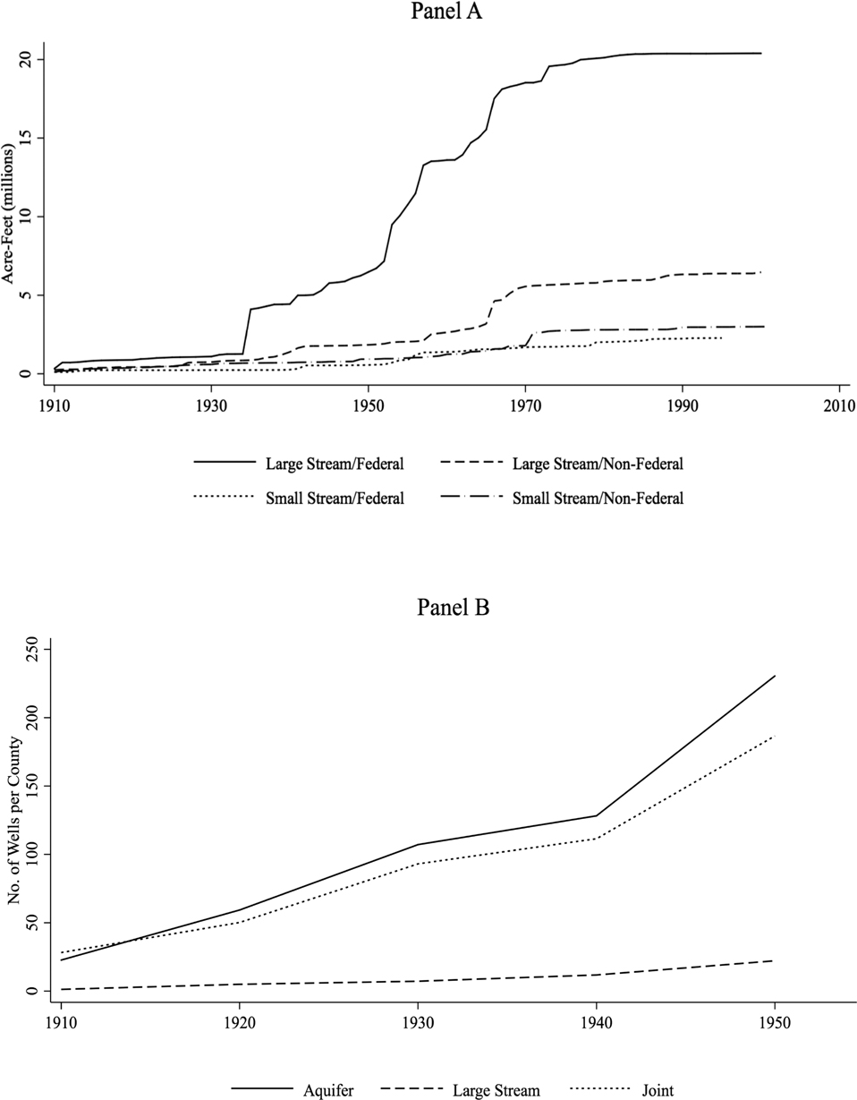
Our empirical strategy relies on the assumption that the exogenous measures of stream size and groundwater are useful in determining where agriculture will have expanded access to water after 1940. We can examine this assumption by looking at correlation and timing between the presence of large streams and groundwater with the presence of dams and wells, respectively. The top panel of Figure 4 shows the cumulative storage behind dams in the western states by federal involvement.Footnote 16 The graph distinguishes storage constructed within counties with large streams from those that have no more than an order 3 stream. Three facts are apparent: Most of the construction occurs (1) on streams of order 4 or larger; (2) on federal projects; and (3) post-1940.Footnote 17 The main exception is in 1936 when the Hoover Dam is completed, providing the initial jump prior to 1940. Furthermore, most of the construction takes place from 1950 to 1980. We also provide statistical support for this positive correlation in the Online Appendix.Footnote 18 On net, the evidence supports our contention that counties with larger streams see more dam construction after 1940.
Expansion of Water Sources

Unlike data on well density discussed later, dam location and storage are available throughout our sample, seemingly allowing for an actual two-stage least square estimation. However, dam location and location of irrigated land are not one in the same. For instance, the South Platte area shown in Figure 3 receives BOR water from reservoirs built on the Colorado River on the other side of the continental divide. Certainly, this is an extreme case, and more often the water is distributed more immediately downstream. Using data from 1950, we find a slight positive relationship between a dam in a county and the acres irrigated by irrigation districts or directly by the BOR. More importantly, however, 69 counties with no federal storage within their borders have acres irrigated by government organizations while 28 counties with federal storage have no acres irrigated by governmental organizations.Footnote 19 Therefore a more precise first-stage test is whether our measure of large stream access predicts the extent of government irrigation, particularly after 1940, but this metric is only reported by county in the 1910 and 1950 censuses. Nonetheless, regression results (reported in the Online Appendix, Table A5) show that our large stream measure predicts the presence of more government irrigation organizations and acres in a county after 1940. Therefore, access to a large stream does increase the odds of receiving stored surface water through government irrigation organizations, even if a dam is not constructed within a county’s borders.Footnote 20 Still, our use of the physical buffer around large streams means that our estimates encompass not only the potential increased supply of surface water, but also the additional protection from floods, which could induce expanded cultivation in previously high flood prone areas.
Turning to groundwater, the time series for well adoption extends only through 1950, but the evidence does support the assumption that aquifer access is predictive of well adoption. In the bottom panel of Figure 4 we show the average number of wells per county over time, grouping counties by the type of water access that has the largest presence in the county.Footnote 21 The counties with access to groundwater by our physical definition, whether or not they also have access to large streams, tend to have more wells. And, while there is an upward trend from 1910 to 1940, there is a marked increase between 1940 and 1950. We support the visual representation with regression results for the number of wells in the county (reported in the Online Appendix, Table A6). In sum, the evidence supports our use of physical access to certain water-types to predict the uptake of wells to access groundwater or the access to water impounded by the proliferation of dams from 1940 onward.
Results
Agricultural Outcomes
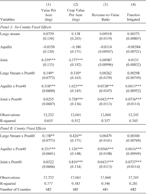
Results for the primary specification, with and without county fixed effects, are provided in Table 2. We focus on Panel A because the estimated impacts for post-1940 are quite stable between the models, and foregoing fixed effects exposes an interesting result in the 1910–1940 period. The coefficients reflect a log-linear specification, where the percentage change in the logged dependent variable is
 ${e^{\hat \eta }} - 1$
, where
 $\hat \eta $
is a coefficient estimate. These results represent the average affect for an acre of land with access to the relevant water source, relative to an acre with access to only small streams.
Estimated Impact of Water Access

Note: Water access is measured by the physical fraction of the county overlaying a water resource. Large stream access is defined by the area within 15 miles of an order stream 4 or higher stream. Additional but unreported controls are state fixed effects, year fixed effects and year fixed effects interacted with: average precipitation, soil quality, elevation, slope mean and range, latitude, longitude, and 1910 population. Sample includes 18 census years from 1910 to 2007. Robust standard errors clustered by county in parentheses.
*** p < 0.01
** p < 0.05
* p < 0.1
Source: Authors’ econometric estimates, see text for details.
Prior to the 1945 census, having access to larger streams or groundwater on their own, according to the estimated coefficients, did not result in more irrigation, crop value, or overall land value relative to baseline areas with only access to smaller streams. Having access to both large streams and groundwater simultaneously, however, increased crop value and land value substantially; relative to land with only small stream access, joint access areas see increased crop and land value of more than 75 percent. To find the effect on the average county, coefficients should be multiplied by the percentage of the county in each access category before making the conversion. For the entire West, the average county has 36 percent of its area over an aquifer, 15 percent of its area in the stream buffer, and 22 percent of its area in both. Thus, the average county would see a land value premium of e 0.559·0.22 – 1 = 13.1 percent as a result of its joint access.
The pre-1945 coefficient on joint access is not driven by earlier ground-water development in California alone, as the advantage of joint access emerges in all three sub regions. This suggests significant advantages exist to large streams when combined with the presence of groundwater even prior to the widespread development of wells and large surface water storage efforts. We look into this unexpected result in some detail later. Meanwhile, after 1940, access to large streams increases land values by 16 percent more relative to changes near small streams (column (1)). This increase, however, is surpassed by land with access to ground-water, which increased in value by 37 percent.Footnote 22 No additional value is capitalized into the land having access to both sources, though it remains more valuable on net.
Shown in column (2), all three treatments derive higher valued crop production per acre after 1940. Crop value premiums for large stream access are the smallest, but still increase a substantial 36 percent relative to increases in crop value of land without large stream or groundwater access in the West. Land overlaying an aquifer increased crop values per acre by a staggering 178 percent. Even when scaling access to the “average” county, crop production values are 44 percent larger on average where groundwater exists. This is true whether or not the land also has access to a large stream (the point estimate on “both” corresponds to 113 percent, but is statistically indistinguishable from groundwater access alone). Paired with the results from column (1) on land value, a puzzle emerges as to why the increased crop value does not translate fully into higher farm values in general and in particular for land with access to both. In general, gains in crop production are significantly larger than gains in land value.
To examine this question we run a regression using the revenue-to-value ratio, that is, crop value divided by farm value, in column (3). Ideally, we would divide agricultural profit by land value to arrive at an imputed discount rate. Using revenue, which is necessitated by a lack of cost data availability, creates a slightly more complicated interpretation: our ratio describes how efficiently agricultural revenues are incorporated into land price. An increase in the ratio as a result of changes in irrigation technology suggests more future uncertainty or a higher cost, as a percentage of revenue, associated with a change in water input technology. In the pre-period there are no statistically significant differences in capitalization ratios across water access. In the post-period, capitalization ratios rise 4–5 percentage points for a county with 100 percent access to groundwater or both large stream and groundwater, but remain steady for areas with just large streams (relative to just small streams). Both explanatory channels seem reasonable: (1) groundwater users receive large contemporaneous benefits from the groundwater, but are discounting the future value of that stock due to the common-pool issues, making the welfare gains smaller because the production gains are offset by losses in the water stock and uncertainty over its future; and (2) though surface reservoirs are generally more expensive than the investment in a center pivot and pumps, the latter is heavily subsidized while the former is typically borne fully by the farmer, reducing the profit margin as revenues increase. Our available data, however, does not permit us to distinguish which explanation is more prominent in explaining our results.
The results in column (4) suggest that larger increases in crop value for groundwater areas relative to large stream areas are likely attributable to new land being brought under irrigation; post-1940 land with groundwater access increases the percent irrigated by 6–7 percentage points, compared to an average of 2 percent prior to 1945. This suggests it may also be the new land brought into irrigated production via groundwater whose revenue is capitalized less efficiently into land value. In contrast, having access to a large stream did not tend to increase irrigated acreage. This suggests that federal projects, on average, may not have resulted in reclamation so much as they served to increase and stabilize water supply for existing acreage. Some expansion of irrigated acreage, however, did occur in the Plain and Pacific states after 1940. A series of robustness checks are presented in the Online Appendix, Tables A8 (stream buffer size) and A9 (controls and sample restrictions). Overall the results are qualitatively robust and rather stable once the main covariates are introduced.Footnote 23
Joint Access Prior to Wells and Dams
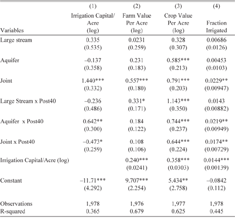
Prior to 1940, even controlling for soil quality and topography, proximity to large streams and aquifers simultaneously provided a significant premium in crop production and land values. We postulate that these lands had more access to groundwater springs due to baseflow, even during periods of drought. Therefore, irrigation was made easier and more productive immediately. Areas with jointly located large streams and aquifers may have had more productive and valuable land due to the presence of near-surface water tables than areas with either the large stream or the groundwater access missing. Furthermore, with less water needed per land unit given the higher water table, the existing stream supply could have brought more land under irrigation. Though we are unable to test this directly using economic data, we can instead look at irrigation investment. Data on this is limited to 1910–1950 due to reporting.
Table 3 reports regression results for variations of equation (2) including irrigation capital investment. Column (1) reports results when capital investment is the dependent variable. Consistent with our empirical framework, areas with only aquifer access see a relative capital influx only after 1940. More importantly, for the matter at hand, acres with joint access attracted more than 322 percent greater investment prior to 1940.Footnote 24 The additional investment is consistent with the notion that irrigation investment was more productive on these lands, even prior to groundwater pumping. Columns (2)–(4) report regression results for the three main outcome variables, now including capital investment as a control variable. As expected, irrigation investment is associated with more irrigated acres, greater crop values, and greater land values. But even controlling for the investment, areas with joint access derive more of these benefits. Further evidence is provided in Table A10 of the Online Appendix where areas with joint access had more land in farms and more improved acres even going back to 1860–1900. While these areas did attract more investment and development, the results in Table 2 find that the extra production was completely reflected in the land value, suggesting the use of the aquifer was relatively cheap and free from common-pool issues, consistent with the groundwater yielding more incidental use than purposeful extraction.
Irrigation Capital Investment and Impact (1910–1950)

Note: Water access is measured by the physical fraction of the county overlaying a water resource. Large Stream is defined by the area within 15 miles of an order stream 4 or higher stream. Additional but unreported controls are state fixed effects, year fixed effects, and year fixed effects interacted with: average precipitation, soil quality, elevation, slope mean and range, latitude, longitude, and 1910 population. Sample includes five census years from 1910 to 1950. Robust standard errors clustered by county in parentheses.
*** p< 0.01
** p < 0.05
* p < 0.1
Source: Authors’ econometric estimates, see text for details.
To this point, we have treated aquifers as a uniform resource capable of providing irrigation water. However, well yield, the measure of how much water can be withdrawn from a well over time, is an important measure of aquifer suitability for irrigation. “The yield of a completed well is probably the most important single item of interest to the well driller…[and] will determine whether or not the well is a success or a failure” (Drillers Journal 1955, p. 9). We examine the well yield of individual aquifers to further characterize why counties with joint access saw crop and land value advantages prior to 1940, as well as to more fully characterize the results from Table 2. Well yield is closely tied to the extent water is mobile under the surface, a property known as hydraulic conductivity. Streams with groundwater systems with low hydraulic conductivity have low baseflow and have “unreliable supplies of water” while areas where streams interact with high conductivity aquifer systems see “relatively stable flow” as a result of baseflow (Winter Reference Winter2007, p. 16). In addition, where large streams and an aquifer coexist, well yields tend to be higher than where an aquifer is the sole supply. This is borne out in our data with cross-sectional regressions that find areas with more joint access having higher yields on average, even controlling for other physical characteristics (presented in Table A11 of the Online Appendix).Footnote 25 Thus, the surface water flow is more reliable in joint access areas than in areas with only stream access, and we can speculate that the reason irrigation infrastructure investment went preferentially to areas with access to both was due to the greater reliability of stream flow in these areas.
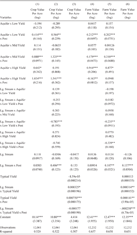
Higher well yield is expected to allow for more groundwater production and thus larger changes post-1940. Table 4 shows the results of estimating equation 2 for both crop value and land value, but with the water access explanatory variables modified to address well yield heterogeneity. Column (1) shows the results of regressing crop value on our aquifer access measure interacted with indicator variables for three distinct bins based on typical well yields and a binary measure of surface water, equal to one if the county contains any portion of an order 4 or higher stream. Column (2) interacts the large stream availability variable with measures of well yield. Column (3) then interacts a continuous measure of well yield with the large stream indicator. All specifications tell a consistent story: post-1940 all types of aquifers increase crop production, and higher well yield leads to higher valued crop production.
Aquifer Yield Heterogeneity

Note: Aquifer access is measured by the fraction of the county overlaying an aquifer, interacted with an indicator variable for the range of typical well yield. Bins are defined by gallons per minute as: low=(0,300], mid=(300,750], and high=(750, 2500]. Alternatively, typical yield is directly used for the measure of aquifer access in columns (4) and (8). Large (Lg.) Stream access is defined by a binary indicator that is one if an order 4 or higher stream is present in the county. Additional but unreported controls are state fixed effects, year fixed effects, and year fixed effects interacted with: average precipitation, soil quality, elevation, slope mean and range, latitude, longitude, and 1910 population. Sample includes 18 census years from 1910 to 2007. Robust standard errors clustered by county in parentheses.
*** p < 0.01
** p < 0.05
* p < 0.1
Source: Authors’ econometric estimates, see text for details.
Columns (4)–(6) show similar results for land value, except that the highest yield aquifers, those with well yields more than 800 gallons per minute, do not show the same post-1940 land value increase, instead showing higher value pre-1940 with no significant change post. This is the same pre-development effect discussed earlier, and columns (3) and (6) shed some light on where the effect is coming from. Crop and land value are increasing in well yield post-1940, but the interaction between large stream presence and yield is positive pre-1940 and statistically significant at the 5 percent level for land value and 10 percent level for crop value. In column (6), the magnitude of this increase is mostly offset by the negative post-1940 interaction between well yield and the large stream indicator. Taken together, these results suggest that it is counties over the highest yield aquifers that see pre-1940 gains, especially those that also have large streams, apparently benefiting from groundwater baseflow, which led to greater reliability in surface water availability even prior to direct access of the aquifer.
Heterogeneous Impacts over Time
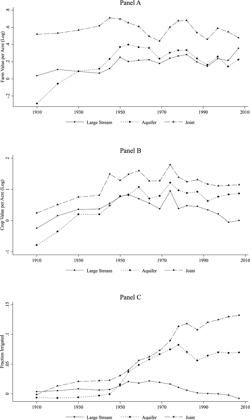
To better understand the evolution of irrigation by type of water source in the West, we estimate equation (3), allowing the coefficient on water access to vary in each year, no longer imposing a break in 1940. We present a visual summary in Figure 5, and the full results are provided in Table A12 of the Online Appendix. The top panel, showing the estimated coefficients of water access each year relative to small streams when farm value is the dependent variable, reveals some additional information beyond the results in Table 2. While the premium for having joint access exists from the very beginning, we also notice that having access to only groundwater appears to be disadvantageous in at least 1910—likely as a result of settlement patterns unrelated to groundwater.Footnote 26 Overall, although the value of aquifer access was already on an upward trend from 1910 to 1930, there is a marked jump following 1940. The added value of aquifer access appears to be capitalized quickly, peaking by 1954, remaining flat or slightly downward afterwards. Large stream access, though not a disadvantage in the pre-period, also jumps up from 1940 to 1950 before flattening out. Joint access, on the other hand, showed some signs of an increase in value from 1940 to 1945, but the gains do not persist beyond 1960 and the value premium remained relatively flat overall, though notably higher than large stream or groundwater access alone.
Estimated Impact of Water Access by Year

Turning to the middle panel, we find similar but distinct patterns in crop production. Crop value premiums by all water access types were trending upward, but noticeably increased following 1940. These gains persist for groundwater and joint access, but appear to dissipate near the end of our sample for large stream access. The bottom panel shows areas with access to large streams, especially where aquifers are jointly present, brought more land under irrigation prior to 1940. Large stream access, however, tends to lose its additional irrigated land after the 1960s, explaining why, on average, no effect was found in Table 2. Having access to groundwater, whether accompanied by access to large streams or not, follows an increasing trajectory in irrigated land until 1980, when aquifer only flattens out while joint access continues to add irrigated acres.
Contrasting the trends in the three panels, while irrigated acres for joint and groundwater access continue to increase relative to small stream areas through the post-1940 period, land value and crop values do not continue to increase in tandem. Land value, as a forward-looking measure, would capitalize expected future gains earlier, and therefore the observed trend is not as surprising as the lack of crop production gains. The lack of further increase in crop value relative to areas with access to small streams is due to at least two reasons, both of which would also explain the flat land value premium: (1) our measure of crop production is a market value, meaning as more land shifts into water-intensive crops, revenue increases due to higher yields are offset by lower market prices; and, (2) other green revolution technologies, including drought-resistant crop varieties and better water management practices, dampen the yield gains of irrigation relative to non-irrigated land over time. Additionally, the land value premium would also stagnate because the land that is brought under irrigation later may be relatively costlier to irrigate, explaining the delay.
Structural Changes
To assess how water access impacts the extent and structure of agricultural activity, we estimate equation (2) for three additional outcome variables: farms per county acre, fraction of county in farms, and the average acreage in a farm (full results provided in the Online Appendix, Table A14). A key finding is that pre-1945, counties with joint access had more farms per acre and more land in farms. This is consistent with our argument that these types of lands, near a large stream with ground-water beneath, attracted more agricultural settlement initially. Following 1940, more farmland was added in areas with large streams and/or groundwater compared to areas with only small streams. In large stream areas the farmland appears to come from farms getting larger, as there is no evidence of more farms per acre while the average farm size increases. This growth occurred despite the land limitations that were to accompany BOR irrigation water. In contrast, increased access to groundwater alone led to more farms per acre, smaller farms, and, on net, more farm acres. By providing decentralized access to irrigation water, groundwater allowed more irrigation by more farmers, while the large centralized investments required for surface water irrigation increased farm acreage without increasing the number of participants. This change in structure of farm sector is primarily driven by changes in the Plain states and access to the Ogallala aquifer: very little reorganization occurred in the Mountain states based on water access, and, in contrast to the Plain states, the Pacific states generally developed larger farms across all water access following the 1940 break (regressions results by region are shown in Tables A14–A16).
Discussion and Conclusion
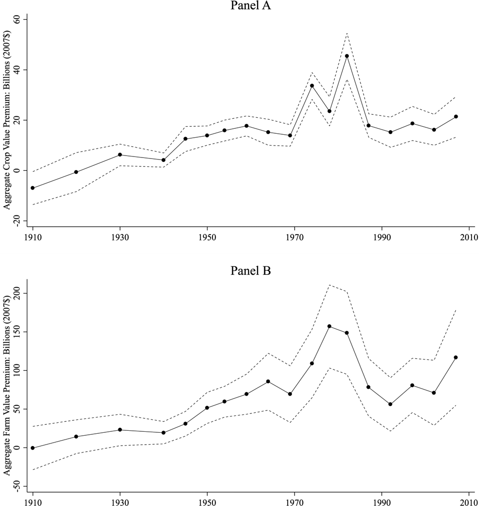
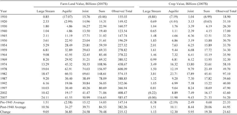
Over the 100 years examined, additional water access provided substantial gains in productivity and value for the arid West. Figure 6 illustrates the combined implied value of large streams and groundwater access relative to areas with only access to small streams based on our estimates over time for those in the West.Footnote 27 Relative gains disaggregated by water type are enumerated in Table 5 (and Figure A11 in the Online Appendix). All told, premiums to crop production on land with access to larger streams, aquifers, or both were virtually non-existent prior to 1940. Post-1940, crop values are notably expanded where access to these differential water sources exist. Our estimates indicate that, on average, areas with greater potential for water development post-1940 produced an additional 19.38 billion dollars of crops annually relative to areas without the same potential (small streams). To put the relative gain in perspective, total crop production in the West increased from an average of $23 billion annually pre-1940 to $45 billion post-1940. The implication is that nearly all the expanded production in this period concentrated where the technological and policy breakthroughs permitted greater groundwater access and construction of dams in the West, albeit possibly at the expense of production elsewhere.
Implied Total Additional Value of Access to Water Beyond Order 3 Streams and Lower for the Western Counties

Implied Value of Water Access

Note: Implied farmland value and crop value is calculated based on coefficient estimates from Figure 5 and observed total farmland valuation by the same process detailed in the text for creating figure 6. “Large Stream,” “Aquifer,” and “Joint” report the total implied value added by these resources beyond the base line of Strahler 3 streams or lower. “Sum” totals these three effects. “Observed Total” reports the total value reported in the census data, aggregated for all counties in the sample.
Source: Authors’ interpretation of econometric estimates, see text for details.
Though we recognize our crop outcome comingles market effects and changing land uses with yields, we contend these results persuasively show that the agricultural production revolution was in no small part attributable to technologies and policies that led to expanded and more reliable irrigation. This is not to dismiss the other factors identified in the literature, but rather that there were likely complementarities and that the other yield-increasing technologies and policies that came about during this period have been especially beneficial to areas with expanded access to water for irrigation. Even areas without irrigation in the West saw some gains in crop production after 1940 and perhaps would have seen more had not expanded water access attracted the bulk of agricultural investment.Footnote 28 More broadly, some of the production gains appear to be result of relocating production from the more humid East (reported in the Online Appendix, Table A18).
Even net of investment, the gains in productivity were in aggregate capitalized into farmland values. The counterfactual for land value is provided in the bottom panel of Figure 6. No premium over access to only smaller streams is statistically identified until after 1940, but since then, access to large streams and aquifers has been immensely valuable. At the peak in 1978, western counties with access to large streams, groundwater, or both had their farm value buoyed by $157 billion relative to areas with only small streams. This relative premium is equal to 26 percent of the total farm value in the West but just 7 percent when considering the East as well. These numbers provide an implicit reminder that while expanded irrigation was important to the West, farms in the East still account for nearly 75 percent of total farmland value. Even where irrigated areas in the West nearly match eastern production, the latter remain more valuable, at least partially due to expense of irrigation.
The timing, and notable peak from 1978–1982, of the land premium match that identified by Hornbeck and Keskin (Reference Hornbeck and Keskin2014), but across all water types, suggesting a macro-driven bubble (Lamm Reference Lamm1997) that disproportionately affected irrigated land and not a particular decline in the value of a specific water source type.Footnote 29 However, there are important distinctions by the type of water access present. Generally, aquifer access alone produces the largest crop premium, but access to both generates the largest farmland value premium. The difference is presumably due to relative costs. Whether this is due to inherently cheaper water that surface sources provide or represents the subsidization of the infrastructure projects is not discernable within our framework. However, given other literature that has critiqued the extensive subsidized water provided irrigators through BOR projects, many times upward of 90 percent of the costs (Wahl Reference Wahl1989, table 2-3, p. 35), our evidence suggests that these irrigators were able to increase production, but enjoyed private gains in land valuations that were proportionally larger than others that increased crop production without the aid of BOR projects. This is evidenced by the fact that large stream access more efficiently translated crop production into land values, consistent with additional costs of expansion not being fully borne by the farmers.
All three regions experienced relative gains in crop production after 1940 related to aquifer access, but only the Plains experienced similar gains for large stream access independent of aquifer access.Footnote 30 More generally, the magnitude of relative gains is largest in the Pacific and the smallest in the Mountain region. Land values also increased in all three regions, but with a significant lag in the Mountain region, suggesting initial higher costs of development in that region offset the crop gains.
Finally, Figure 6 casts doubt that the premium for irrigation access is waning. In fact, 2007 had the third largest estimated land premium, suggesting stored water may have a significant role as the impacts of climate change are felt by western farms. Furthermore, it is surface water access that saw its largest relative premium in 2007, indicating the value of renewable storage may yet be on the rise long after dam construction stopped. Irrigation, in fact, continues to expand in the United States, though most in the more humid East: since 1978 the West has hovered around 40 million irrigated acreage while the East expanded from 10 million to 18 million irrigated acres, now accounting for nearly one-third of all irrigated acreage in the United States.Footnote 31 Putting these eastern counties into our framework (reported in the Online Appendix, Table A18), we found that land premiums also increased in the East, largely from groundwater access, though not as much as they did in the West. Furthermore, crop production in the East did not increase. One explanation could be that irrigation provides a type of insurance in a changing climate, even if production on average is not enhanced.
While, breakthroughs in technology and rural electrification around 1940 increased farm productivity across the entire United States, our results indicate that, among the arid region, benefits were bolstered or concentrated in regions where expanded water access was made possible around the same time. Considering its important role in the agricultural history of the United States and concerns about a changing climate, irrigation should remain a central concern to future policy discussions. This is especially true in developing nations where natural water supplies will be put in greater peril by climate change. Our results further indicate that efforts to regulate groundwater extraction may be most important, as only 6 percent of the water-access production gains identified in this article stem from surface water access exclusively. Therefore, investing in the development of institutions for the sound management of an existing pool of water—surface or ground—may be more cost-effective than creating new pools of water through expensive surface water infrastructure.