1 Introduction
Reynolds-averaged Navier–Stokes (RANS) models are widely used because of their computational tractability. Most two-equation RANS models rely on the linear eddy viscosity model (LEVM) for their Reynolds stress closure. The LEVM postulates a linear relationship between the Reynolds stresses and the mean strain rate. However, this model does not provide satisfactory predictive accuracy in many engineering-relevant flows, such as those with curvature, impingement and separation (Craft, Launder & Suga Reference Craft, Launder and Suga1996). In particular, it has been demonstrated that the LEVM does not capture the correct Reynolds stress anisotropy in many flows, including simple shear flows (Tracey, Duraisamy & Alonso Reference Tracey, Duraisamy and Alonso2013). More advanced nonlinear eddy viscosity models have also been proposed (Pope Reference Pope1975; Craft et al. Reference Craft, Launder and Suga1996; Wallin & Johansson Reference Wallin and Johansson2000) which rely on higher-order products of the mean strain rate and rotation rate tensors. These nonlinear models have not gained widespread usage because they do not give consistent performance improvement over the LEVM and often lead to worsened convergence properties (Gatski & Speziale Reference Gatski and Speziale1993).
More recently, there has been interest in using machine learning methods to develop Reynolds stress closures. Tracey et al. (Reference Tracey, Duraisamy and Alonso2013) used kernel regression to model the Reynolds stress anisotropy eigenvalues. This method was shown to have limited ability to generalize to new flows and to scale to large amounts of training data. Tracey, Duraisamy & Alonso (Reference Tracey, Duraisamy and Alonso2015) later used neural networks with a single hidden layer to model the source terms from the Spalart Allmaras RANS model. These neural networks were shown capable of reconstructing these source terms, demonstrating the potential utility of neural networks for turbulence modelling. Zhang & Duraisamy (Reference Zhang and Duraisamy2015) used neural networks to predict a correction factor for the turbulent production term. This correction term could affect the magnitude but not the anisotropy of the predicted Reynolds stress tensor. Ling et al. (Reference Ling, Ruiz, Lacaze and Oefelein2016b ) proposed the use of random forests to predict the Reynolds stress anisotropy. However, random forests are limited in their ability to predict the full anisotropy tensor because they cannot easily enforce Galilean invariance for a tensor quantity.
Deep learning presents an attractive alternative for modelling the Reynolds stresses. Deep learning with deep neural networks is a branch of machine learning in which input features are transformed through multiple layers of nonlinear interactions (LeCun, Bengio & Hinton Reference Lecun, Bengio and Hinton2015). Deep neural networks have gained attention for their ability to represent complex interactions and achieve superior results across a wide range of applications, including video classification (Karpathy et al. Reference Karpathy, Toderici, Shetty, Leung, Sukthankar and Li2014), voice recognition (Hinton et al. Reference Hinton2012), and playing the game of Go (Silver et al. Reference Silver2016). Despite the widespread success of neural networks at providing high-quality predictions in complex problems, there have been only limited attempts to apply deep learning techniques to turbulence modelling. Tracey et al. (Reference Tracey, Duraisamy and Alonso2013) and Zhang & Duraisamy (Reference Zhang and Duraisamy2015) used neural networks with only one or two hidden layers. Milano & Koumoutsakos (Reference Milano and Koumoutsakos2002) used neural networks with multiple hidden layers to replicate near-wall channel flows, but did not build these neural networks into forward models for turbulent flow prediction. This paper will demonstrate that deep neural networks can provide improved Reynolds stress closures.
A key strength of neural networks is in the flexibility of their architecture. While random forests cannot easily be restructured to preserve tensor invariance properties, neural networks can be. Ling, Jones & Templeton (Reference Ling, Jones and Templeton2016a ) used neural networks to predict the Reynolds stress anisotropy eigenvalues, and reported significant performance gains when a rotationally invariant input feature set was used. These results showed that embedding invariance properties into the machine learning model is critical for achieving high performance. In the current work, a specialized neural network architecture is proposed which embeds Galilean invariance into the neural network predictions. This neural network is able to predict not only the anisotropy eigenvalues, but the full anisotropy tensor while preserving Galilean invariance. The neural network model is trained and evaluated on a database of flows for which both RANS and high-fidelity (direct numerical simulation (DNS) or well-resolved large eddy simulation (LES)) data are available. The performance of this specialized neural network is compared with that of a more generic feed-forward multilayer perceptron (MLP) that does not embed Galilean invariance.
Section 2 will introduce the concepts of deep neural networks and will present the architecture for the MLP and the specialized invariant neural network. Section 3 will detail the data sets used for training, validation and testing. Section 4 will present the neural network predictions of the Reynolds stress anisotropy as well as the velocity fields calculated when using these anisotropy values. Finally, § 5 will present conclusions and ideas for next steps.
2 Deep neural networks
Neural networks are composed of connected nodes. Each node takes in inputs
 $\boldsymbol{x}$
, transforms the inputs through an activation function
 $f(\boldsymbol{x})$
and outputs the result. A common activation function, the rectified linear unit (ReLU), is defined as
 $f(\boldsymbol{x})=\max (0,\boldsymbol{w}\boldsymbol{\cdot }\boldsymbol{x})$
. In this expression,
 $\boldsymbol{w}$
is the node weight vector which is set during the training phase of the model. The leaky ReLU activation function is an adaptation of ReLU with a small negative slope for negative values of
 $\boldsymbol{w}\boldsymbol{\cdot }\boldsymbol{x}$
. The leaky ReLU was used in this work because it enables efficient training of deep neural networks (Maas, Hannun & Ng Reference Maas, Hannun and Ng2013). In deep neural networks, there are multiple layers of nodes, with the outputs of one layer becoming the inputs to the next layer. By using multiple layers of transformations, deep neural networks are able to capture complex, hierarchical interactions between features. The layers between the input layer and the output layer are called hidden layers because the physical interpretation of their activation is not always clear.
The inputs to the neural networks were based on the mean strain rate tensor
 $\unicode[STIX]{x1D64E}$
and the mean rotation rate tensor
 $\unicode[STIX]{x1D64D}$
, non-dimensionalized using the turbulent kinetic energy
 $k$
and the turbulent dissipation rate
 $\unicode[STIX]{x1D716}$
as suggested by Pope (Reference Pope1975). The output was the normalized Reynolds stress anisotropy tensor,
 $\unicode[STIX]{x1D657}$
, where
 $\unicode[STIX]{x1D623}_{ij}=\overline{\boldsymbol{u}_{i}^{\prime }\boldsymbol{u}_{j}^{\prime }}/2k-1/3\unicode[STIX]{x1D739}_{ij}$
. The predicted anisotropy was post-processed to ensure realizability by enforcing constraints on
 $\unicode[STIX]{x1D657}$
and its eigenvalues
 $\unicode[STIX]{x1D709}_{1}\geqslant \unicode[STIX]{x1D709}_{2}\geqslant \unicode[STIX]{x1D709}_{3}$
(Banerjee et al.
Reference Banerjee, Kraal, Durst and Zenger2007):
 $$\begin{eqnarray}\left.\begin{array}{@{}ll@{}}-{\textstyle \frac{1}{3}}\leqslant \unicode[STIX]{x1D623}_{ii}\leqslant {\textstyle \frac{2}{3}} & \unicode[STIX]{x1D709}_{1}\geqslant (3|\unicode[STIX]{x1D709}_{2}|-\unicode[STIX]{x1D709}_{2})/2\\ -{\textstyle \frac{1}{2}}\leqslant \unicode[STIX]{x1D623}_{ij}\leqslant {\textstyle \frac{1}{2}}\quad \text{for }j\neq i & \unicode[STIX]{x1D709}_{1}\leqslant {\textstyle \frac{1}{3}}-\unicode[STIX]{x1D709}_{2}.\end{array}\right\}\end{eqnarray}$$
The neural networks were trained using back propagation with gradient descent. The process of training a neural network is analogous to calibrating a regression model. In training, the model is fit to a subset of the data, known as the training data, by iteratively adjusting the node weights to provide the lowest mean squared error between the predicted and true values of the anisotropy tensor.
For both neural network architectures, there were three main hyper-parameters: the number of hidden layers, the number of nodes per hidden layer and the learning rate in the gradient descent training algorithm. All three of these parameters can have a significant effect on model performance. Larger networks (with more hidden layers and more nodes per layer) can fit more complex data, but are also more prone to over-fitting the data. These three hyper-parameters were determined through a Bayesian optimization process, implemented using the Spearmint python package described in detail by Snoek, Larochelle & Adams (Reference Snoek, Larochelle and Adams2012).
In this process, the parameter space was sampled and at each sample, a neural network with those hyper-parameters was constructed and trained. The network performance was then evaluated on a validation data set that was separate from both the training data and the test data. The optimal hyper-parameters were chosen to be those values that yielded the lowest error on this validation set. There was inherent randomness in the model validation error for specific hyper-parameter values because of the randomized network weight initialization and the randomized data set shuffling during gradient descent. The model’s validation error at each hyper-parameter setting was therefore treated as a sample from a Gaussian process (GP). The Bayesian optimization framework is distinguished by requiring relatively fewer model evaluations as compared with many gradient-based optimization techniques, because at each step, the information from all previous steps is used to inform the GP model of the validation error. This method is therefore advantageous when the computational cost of evaluating the objective function is high, as is the case with training a neural network. Through this Bayesian optimization process, the parameter space was efficiently sampled to find the parameters that yielded the best performance on the validation set.
For the two network architectures evaluated, the MLP and the specialized invariant neural network, the optimal number of hidden layers was 10 and 8, respectively. These optimal values correspond to significantly deeper neural networks than have previously been investigated for turbulence modelling. For example, Tracey et al. (Reference Tracey, Duraisamy and Alonso2015) used a network with only two hidden layers. Therefore, these results represent one of the first efforts in using deep neural networks for turbulence modelling. It is not expected that these network hyper-parameters will be universally optimal for predicting any given quantity of interest in turbulence modelling. However, the Bayesian optimization procedure is a general approach for systematically optimizing deep neural network hyper-parameters.
Because the training process of deep neural networks is prone to converge to local minima instead of the global minimum, an ensemble of networks was trained, each with randomly initialized weights. Network training was deemed complete when the model error on a held-out validation set of data stopped decreasing. The ensemble size was 20 networks, which was shown sufficient to provide multiple networks converging to the same minimum validation error. Each network required approximately 200 CPU hours to train, so that the entire ensemble required 4000 CPU hours to train.
2.1 MLP
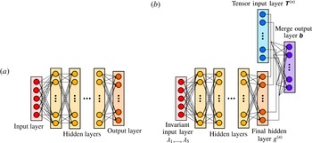
A MLP is the most basic type of neural network: it is a densely connected feed-forward neural network. Feed-forward means that there are no loops in the connections between the nodes. Densely connected means that each node in a given layer is connected to all of the nodes in the next layer. Figure 1(a) shows a schematic of an MLP. The inputs to the MLP were the nine distinct components of the non-dimensionalized strain rate and rotation rate tensors,
 $\unicode[STIX]{x1D64E}$
and
 $\unicode[STIX]{x1D64D}$
, at a given point in the flow as predicted by RANS. Through Bayesian optimization, the network was set to have 10 hidden layers, each with 10 nodes, and the learning rate was
 $2.5\times 10^{-6}$
.
Schematic of neural network architectures.

2.2 Tensor basis neural network
A special network architecture, which will be referred to as the tensor basis neural network (TBNN), is proposed in this paper. This network architecture, shown in figure 1(b), embeds rotational invariance by enforcing that the predicted anisotropy tensor lies on a basis of isotropic tensors. Rotational invariance signifies that the physics of the fluid flow do not depend on the orientation of the coordinate frame of the observer. This is a fundamental physical principle, and it is important that any turbulence closure obeys it. Otherwise, the machine learning model evaluated on identical flows with the axes defined in different directions could yield different predictions.
If the goal were just to predict the eigenvalues of the anisotropy tensor, then a basis of tensor invariants could be used as the input features to ensure the rotational invariance of the predicted eigenvalues, as was done in Ling et al. (Reference Ling, Jones and Templeton2016a ). However, to predict the full anisotropy tensor, this approach is not sufficient. Unlike the anisotropy eigenvalues, the full anisotropy tensor will change when the coordinate axes are rotated. The key to ensuring Galilean invariance is therefore to ensure that when the coordinate frame is rotated, the anisotropy tensor is also rotated by the same angles. Therefore, if the input to the neural network is a rotated velocity gradient tensor, the output should be the corresponding rotated anisotropy tensor. This can be achieved by constructing an integrity basis of the input tensors. Further explanation of integrity bases for isotropic functions can be found in Smith (Reference Smith1965).
For the specific case of interest here, with input tensors
 $\unicode[STIX]{x1D64E}$
and
 $\unicode[STIX]{x1D64D}$
, Pope (Reference Pope1975) has previously derived the relevant integrity basis. Pope proved that in the most general incompressible case, an eddy viscosity model that is a function of only
 $\unicode[STIX]{x1D64E}$
and
 $\unicode[STIX]{x1D64D}$
can be expressed as a linear combination of 10 isotropic basis tensors:
 $$\begin{eqnarray}\displaystyle \unicode[STIX]{x1D657}=\mathop{\sum }_{n=1}^{10}g^{(n)}(\unicode[STIX]{x1D706}_{1},\ldots ,\unicode[STIX]{x1D706}_{5})\unicode[STIX]{x1D64F}^{(n)}. & & \displaystyle\end{eqnarray}$$
Any tensor
 $\unicode[STIX]{x1D657}$
which satisfies this condition will automatically satisfy Galilean invariance. There are only a finite number of tensors because by the Caley–Hamilton theory, higher order products of these two tensors can be reduced to a linear combination of this tensor basis. The five tensor invariants
 $\unicode[STIX]{x1D706}_{1},\ldots ,\unicode[STIX]{x1D706}_{5}$
are known scalar functions of the elements of
 $\unicode[STIX]{x1D64E}$
and
 $\unicode[STIX]{x1D64D}$
. Pope (Reference Pope1975) gave a detailed derivation of these 10 tensors,
 $\unicode[STIX]{x1D64F}^{(1)},\ldots ,\unicode[STIX]{x1D64F}^{(10)}$
and 5 invariants
 $\unicode[STIX]{x1D706}_{1},\ldots ,\unicode[STIX]{x1D706}_{5}$
, which are listed below:
 $$\begin{eqnarray}\left.\begin{array}{@{}ll@{}}\unicode[STIX]{x1D64F}^{(1)}=\unicode[STIX]{x1D64E} & \unicode[STIX]{x1D64F}^{(6)}=\unicode[STIX]{x1D64D}^{2}\unicode[STIX]{x1D64E}+\unicode[STIX]{x1D64E}\unicode[STIX]{x1D64D}^{2}-{\textstyle \frac{2}{3}}\unicode[STIX]{x1D644}\boldsymbol{\cdot }Tr(\unicode[STIX]{x1D64E}\unicode[STIX]{x1D64D}^{2})\\ \unicode[STIX]{x1D64F}^{(2)}=\unicode[STIX]{x1D64E}\unicode[STIX]{x1D64D}-\unicode[STIX]{x1D64D}\unicode[STIX]{x1D64E} & \unicode[STIX]{x1D64F}^{(7)}=\unicode[STIX]{x1D64D}\unicode[STIX]{x1D64E}\unicode[STIX]{x1D64D}^{2}-\unicode[STIX]{x1D64D}^{2}\unicode[STIX]{x1D64E}\unicode[STIX]{x1D64D}\\ \unicode[STIX]{x1D64F}^{(3)}=\unicode[STIX]{x1D64E}^{2}-{\textstyle \frac{1}{3}}\unicode[STIX]{x1D644}\boldsymbol{\cdot }Tr(\unicode[STIX]{x1D64E}^{2}) & \unicode[STIX]{x1D64F}^{(8)}=\unicode[STIX]{x1D64E}\unicode[STIX]{x1D64D}\unicode[STIX]{x1D64E}^{2}-\unicode[STIX]{x1D64E}^{2}\unicode[STIX]{x1D64D}\unicode[STIX]{x1D64E}\\ \unicode[STIX]{x1D64F}^{(4)}=\unicode[STIX]{x1D64D}^{2}-{\textstyle \frac{1}{3}}\unicode[STIX]{x1D644}\boldsymbol{\cdot }Tr(\unicode[STIX]{x1D64D}^{2}) & \unicode[STIX]{x1D64F}^{(9)}=\unicode[STIX]{x1D64D}^{2}\unicode[STIX]{x1D64E}^{2}+\unicode[STIX]{x1D64E}^{2}\unicode[STIX]{x1D64D}^{2}-{\textstyle \frac{2}{3}}\unicode[STIX]{x1D644}\boldsymbol{\cdot }Tr(\unicode[STIX]{x1D64E}^{2}\unicode[STIX]{x1D64D}^{2})\\ \unicode[STIX]{x1D64F}^{(5)}=\unicode[STIX]{x1D64D}\unicode[STIX]{x1D64E}^{2}-\unicode[STIX]{x1D64E}^{2}\unicode[STIX]{x1D64D} & \unicode[STIX]{x1D64F}^{(10)}=\unicode[STIX]{x1D64D}\unicode[STIX]{x1D64E}^{2}\unicode[STIX]{x1D64D}^{2}-\unicode[STIX]{x1D64D}^{2}\unicode[STIX]{x1D64E}^{2}\unicode[STIX]{x1D64D}\end{array}\right\}\end{eqnarray}$$
 $$\begin{eqnarray}\displaystyle \unicode[STIX]{x1D706}_{1}=Tr(\unicode[STIX]{x1D64E}^{2}),\quad \unicode[STIX]{x1D706}_{2}=Tr(\unicode[STIX]{x1D64D}^{2}),\quad \unicode[STIX]{x1D706}_{3}=Tr(\unicode[STIX]{x1D64E}^{3}),\quad \unicode[STIX]{x1D706}_{4}=Tr(\unicode[STIX]{x1D64D}^{2}\unicode[STIX]{x1D64E}),\quad \unicode[STIX]{x1D706}_{5}=Tr(\unicode[STIX]{x1D64D}^{2}\unicode[STIX]{x1D64E}^{2}). & & \displaystyle \nonumber\\ \displaystyle & & \displaystyle\end{eqnarray}$$
The goal of the TBNN, then, is to determine the scalar coefficients
 $g^{(n)}(\unicode[STIX]{x1D706}_{1},\ldots ,\unicode[STIX]{x1D706}_{5})$
in (2.2). Once these coefficients are determined, then (2.2) can be used to solve for the anisotropy tensor
 $\unicode[STIX]{x1D657}$
.
As figure 1(b) shows, the network architecture was designed to match (2.2). There are two input layers: an invariant input layer and a tensor input layer. The invariant input layer takes in the invariants
 $\unicode[STIX]{x1D706}_{1},\ldots ,\unicode[STIX]{x1D706}_{5}$
and is followed by a series of hidden layers. The final hidden layer has 10 nodes and represents
 $g^{(n)}$
for
 $n=1,\ldots ,10$
. The tensor input layer also has 10 nodes for the 10 tensors
 $\unicode[STIX]{x1D64F}^{(n)}$
for
 $n=1,\ldots ,10$
. The merge output layer takes the element-wise product of the outputs of the final hidden layer and the tensor input layer and sums the result to give the final prediction for
 $\unicode[STIX]{x1D657}$
. This innovative architecture ensures that (2.2) is satisfied, thereby guaranteeing the Galilean invariance of the network predictions. Through Bayesian optimization, the number of hidden layers was set to 8, with 30 nodes per hidden layer. The learning rate was
 $2.5\times 10^{-7}$
.
3 Data sets
The neural networks were trained, validated and tested on a database of nine flows for which both high fidelity (DNS or well-resolved LES) as well as RANS results were available. The RANS data, obtained using the
 $k{-}\unicode[STIX]{x1D716}$
model with the LEVM for the Reynolds stresses, were used as the inputs to the neural networks. The RANS results, not the DNS results, were used as inputs to the neural network because the neural networks must be able to make predictions in the absence of DNS data. The high-fidelity data were used to provide the truth labels for the Reynolds stress anisotropy during model training and evaluation.
The nine flows in the database were selected because of the availability of high-fidelity data and because they represent canonical flow cases. All of the high-fidelity simulation results have been previously reported in the literature. Six cases were used for training: duct flow at
 $Re_{b}=3500$
(Pinelli et al.
Reference Pinelli, Uhlmann, Sekimoto and Kawahara2010), channel flow at
 $Re_{\unicode[STIX]{x1D70F}}=590$
(Moser, Kim & Mansour Reference Moser, Kim and Mansour1999), a perpendicular jet in cross-flow (Ruiz, Oefelein & Lacaze Reference Ruiz, Oefelein and Lacaze2015), an inclined jet in cross-flow (Ling et al.
Reference Ling, Ryan, Bodart and Eaton2016c
), flow around a square cylinder (Ray et al.
Reference Ray, Lefantzi, Arunajatesan and Dechant2014) and flow through a converging–diverging channel (Marquillie, Ehrenstein & Laval Reference Marquillie, Ehrenstein and Laval2011). One case was used for validation when selecting the neural network hyper-parameters through Bayesian optimization: a wall-mounted cube in cross-flow at bulk Reynolds number of 5000 (Rossi, Philips & Iaccarino Reference Rossi, Philips and Iaccarino2010). Two cases were used for testing: duct flow at
 $Re_{b}=2000$
and flow over a wavy wall at
 $Re=6850$
. These cases were chosen for test sets because they are both flows in which Reynolds stress anisotropy plays a key role.
It is notable that this flow database represents a wide variety of different flow configurations. We are therefore testing the ability of the neural network to do more than just interpolate between similar flow configurations at different Reynolds numbers; we are evaluating the ability of the neural network to learn about the underlying flow regimes present in these configurations.
Predictions of Reynolds stress anisotropy tensor
 $\unicode[STIX]{x1D657}$
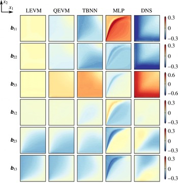
on the duct flow test case. Only the lower left quadrant of the duct is shown, and the streamwise flow direction is out of the page. The columns show the predictions of the LEVM, QEVM, TBNN and MLP models. The true DNS anisotropy values are shown in the right-most column for comparison.

Previous work by Ling & Templeton (Reference Ling and Templeton2015) investigated the effect of the database size on the performance of their Random Forest machine learning models. Their database included seven flow cases, and they showed improved cross-validated model performance when they trained their models on six of the flows versus when they trained on a lower number of the flows in their database. Ling & Templeton (Reference Ling and Templeton2015) also used the Mahalanobis distance to characterize how similar a given test flow was to the training database. They showed that their machine learning models were more accurate in regions that had a lower mean Mahalanobis distance, indicating a stronger similarity in feature space. These results suggest that the choice and size of the training database are both critical to the performance of the machine learning model. Therefore, it will be the aim of future work to train and test these neural networks across a broader range of flows.
4 Results
4.1 A priori results
The MLP and TBNN were used to predict the normalized Reynolds stress anisotropy tensor
 $\unicode[STIX]{x1D657}$
for two different test flow cases: turbulent duct flow and flow over a wavy wall. Figure 2 shows the anisotropy predictions for the duct flow case. For comparison, the anisotropy predictions from two different baseline RANS simulations are also shown. The first RANS was run using the default LEVM:
 $\unicode[STIX]{x1D657}=-\unicode[STIX]{x1D708}_{t}\unicode[STIX]{x1D64E}/k$
. The second RANS used a quadratic eddy viscosity model (QEVM) based on the nonlinear eddy viscosity model of Craft et al. (Reference Craft, Launder and Suga1996):
 $$\begin{eqnarray}\displaystyle \unicode[STIX]{x1D623}_{ij} & = & \displaystyle -\frac{\unicode[STIX]{x1D708}_{t}\unicode[STIX]{x1D61A}_{ij}}{k}+C_{1}\frac{\unicode[STIX]{x1D708}_{t}}{\tilde{\unicode[STIX]{x1D716}}}\left(2\unicode[STIX]{x1D61A}_{ik}\unicode[STIX]{x1D61A}_{kj}-\frac{2}{3}\unicode[STIX]{x1D61A}_{kl}\unicode[STIX]{x1D61A}_{kl}\unicode[STIX]{x1D6FF}_{ij}\right)\nonumber\\ \displaystyle & & \displaystyle +\,C_{2}\frac{\unicode[STIX]{x1D708}_{t}}{\tilde{\unicode[STIX]{x1D716}}}(2\unicode[STIX]{x1D619}_{ik}\unicode[STIX]{x1D61A}_{kj}+2\unicode[STIX]{x1D619}_{jk}\unicode[STIX]{x1D61A}_{ki})+C_{3}\frac{\unicode[STIX]{x1D708}_{t}}{\tilde{\unicode[STIX]{x1D716}}}\left(2\unicode[STIX]{x1D619}_{ik}\unicode[STIX]{x1D619}_{jk}-\frac{2}{3}\unicode[STIX]{x1D619}_{kl}\unicode[STIX]{x1D619}_{kl}\unicode[STIX]{x1D6FF}_{ij}\right).\end{eqnarray}$$
In this model, the coefficients are set as
 $C_{1}=-0.1$
,
 $C_{2}=0.1$
, and
 $C_{3}=0.26$
.
As figure 2 shows, the baseline LEVM completely failed to predict the anisotropy values. It predicted zero anisotropy for
 $\unicode[STIX]{x1D623}_{11}$
,
 $\unicode[STIX]{x1D623}_{22}$
,
 $\unicode[STIX]{x1D623}_{33}$
and
 $\unicode[STIX]{x1D623}_{12}$
. This is due to the fact that the LEVM does not predict any secondary flows in the duct, so the mean velocity in the
 $x_{1}$
and
 $x_{2}$
directions is zero, causing
 $\unicode[STIX]{x1D61A}_{11}$
,
 $\unicode[STIX]{x1D61A}_{22}$
and
 $\unicode[STIX]{x1D61A}_{12}$
to be zero. Since the flow is periodic in the
 $x_{3}$
direction,
 $\unicode[STIX]{x1D61A}_{33}$
is also zero. As a result, the corresponding
 $\unicode[STIX]{x1D657}$
components are zero, as shown. The QEVM does slightly better, predicting the right sign, though still too small a magnitude, for these components of
 $\unicode[STIX]{x1D657}$
. The TBNN does even better, getting closer to the correct magnitude for these components of
 $\unicode[STIX]{x1D657}$
. The MLP, on the other hand, completely fails to predict the anisotropy in this configuration. Its predictions are both qualitatively and quantitatively inaccurate.
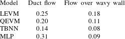
A more quantitative comparison of these model performances is given by table 1, which provides the root mean squared error (RMSE) for these four models with respect to the DNS data. The RMSE was calculated by summing over all of the points in the RANS mesh and all of the distinct components of
 $\unicode[STIX]{x1D657}$
:
 $$\begin{eqnarray}\displaystyle \text{RMSE}=\sqrt{\frac{1}{6N_{data}}\mathop{\sum }_{\text{m=1}}^{N_{data}}\mathop{\sum }_{i=1}^{3}\mathop{\sum }_{j=1}^{i}(\unicode[STIX]{x1D623}_{ij,m,\mathit{predicted}}-\unicode[STIX]{x1D623}_{ij,m,\mathit{DNS}})^{2}}. & & \displaystyle\end{eqnarray}$$
This table confirms that the TBNN provides by far the most accurate predictions in this case: 44 % and 30 % lower error than the LEVM and QEVM, respectively.
Root mean squared error on test cases.

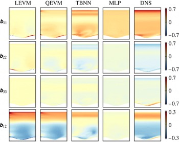
Figure 3 shows the anisotropy predictions on the wavy wall test case. Here
 $\unicode[STIX]{x1D623}_{13}$
and
 $\unicode[STIX]{x1D623}_{23}$
are not shown because they are identically zero in this two-dimensional test case. Once again, the LEVM is unable to predict even the qualitative trends in the anisotropy components, and the QEVM is only slightly better, predicting the correct sign for the on-diagonal components of
 $\unicode[STIX]{x1D657}$
. The TBNN predicts closer to the correct magnitude for the on-diagonal components of
 $\unicode[STIX]{x1D657}$
. For the
 $\unicode[STIX]{x1D623}_{12}$
component, it predicts too low of anisotropy near the center of the channel. On the other hand, it does not overpredict the anisotropy in the very near-wall region, as the LEVM and QEVM do. Once again, the MLP is unable to make satisfactory predictions for the anisotropy in this flow.
Predictions of Reynolds stress anisotropy
 $\unicode[STIX]{x1D657}$
tensor on the wavy wall test case. The columns show the predictions of the LEVM, QEVM, TBNN and MLP models. The true DNS anisotropy values are shown in the right-most column for comparison.

Table 1 lists the RMSE values for each of the four models in the wavy wall test case. Once again, the TBNN provides the predictions with the lowest error, giving a 56 % reduction in error with respect to LEVM and a 27 % reduction in error with respect to QEVM. The majority of this reduction in error was due to improved accuracy in the
 $\unicode[STIX]{x1D623}_{11}$
and
 $\unicode[STIX]{x1D623}_{22}$
components. In this case, the MLP surpasses LEVM and QEVM, but still falls short of the TBNN in accuracy. Therefore, on both test cases, the TBNN has been shown to provide substantial reductions in error with respect to the baseline RANS models. The TBNN has also been shown to be consistently more accurate than the MLP, emphasizing the performance benefits of embedding invariance into the network architecture.
In order to evaluate the TBNN performance across a broader range of flows, an additional set of validation tests were performed, using leave-one-out cross-validation. In this cross-validation technique, each of the six flows originally in the training set was used once as the test case. The TBNN was retrained on the flow data base excluding this test flow. Therefore, as always, the TBNN was evaluated on a flow that was not used for training. For all cross-validation cases, the same hyper-parameters (8 layers, 30 nodes per layer) were used. In all six cross-validation cases, the TBNN provided lower error than the default LEVM. On average, the TBNN reduced the RMSE by 30 % compared with the LEVM. These cross-validation results provide evidence of the generality and robustness of the TBNN approach.
4.2 A posteriori results
Given the significantly improved Reynolds stress anisotropy predictions of the TBNN, it was of interest to determine whether these improved anisotropy values would translate to improved mean velocity predictions. Therefore, the Reynolds stress anisotropy tensor predicted by the TBNN was implemented in an in-house RANS solver, SIERRA Fuego (Domino et al.
Reference Domino, Moen, Burns and Evans2003), in the momentum equations and in the turbulent kinetic energy production term. The RANS solver was first allowed to reach convergence using the default LEVM, and the TBNN Reynolds stress anisotropy predictions were then prescribed and the simulation was allowed to re-converge. After the TBNN stresses were injected, the simulation residuals converged to less than
 $10^{-7}$
for the momentum and continuity equations and to less than
 $10^{-4}$
for the turbulence quantities. This was the same order of magnitude of residuals that was reached when the default LEVM was used to provide the stresses. Future studies will investigate the feasibility of iterative convergence, in which the TBNN is queried at every iteration.
Notably, the Reynolds stress anisotropy is not the only source of uncertainty in the RANS equations, which also rely on approximate transport equations for
 $k$
and
 $\unicode[STIX]{x1D716}$
. Therefore, the true DNS anisotropy values were also implemented in the RANS solver as fixed fields as a point of comparison. This DNS anisotropy (DNS-
 $\unicode[STIX]{x1D657}$
) model shows the flow predictions that would be achieved by using the correct normalized anisotropy tensor
 $\unicode[STIX]{x1D657}$
, given the other RANS model assumptions. It therefore represents the upper performance limit of an improved Reynolds stress anisotropy model.
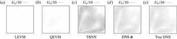
In the duct flow test case, one of the major failings of LEVM is that it cannot predict the corner vortices that are known to form in this flow. Figure 4 shows the secondary flow predictions made by the LEVM, QEVM, TBNN, DNS-
 $\unicode[STIX]{x1D657}$
, and the true DNS. As this figure shows, the LEVM does not predict any secondary flows at all. The QEVM predicts corner vortices, but significantly underpredicts their strength. The TBNN, on the other hand, slightly overpredicts the strength of the corner vortices. The DNS-
 $\unicode[STIX]{x1D657}$
is the most accurate in predicting the strength of the vortices. In this test case, then, the TBNN provides improved but still imperfect secondary flow predictions.
Plot of secondary flows in duct flow case. Reference arrows of length
 $U_{b}/10$
shown at the top of each plot.

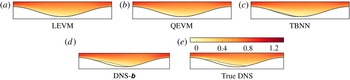
In the case of periodic flow over a wavy wall, the DNS shows flow separation on the leeward side of the bump. RANS struggles to correctly capture this separation region. Figure 5 shows contours of streamwise velocity for this flow case. The RANS LEVM and QEVM both fail to predict flow separation downstream of the bump. The DNS-
 $\unicode[STIX]{x1D657}$
correctly predicts the size and shape of the separated region. TBNN successfully predicts flow separation, albeit over a smaller region than the DNS.
Contours of streamwise velocity normalized by bulk velocity in the wavy wall test case, zoomed into the near-wall region. Separated regions outlined in grey.

In both test cases, the TBNN’s more accurate Reynolds stress anisotropy predictions yielded improved mean velocity predictions in comparison with RANS LEVM and QEVM. On the other hand, there is still room for improvement, as is shown by the DNS-
 $\unicode[STIX]{x1D657}$
results. The improved accuracy of DNS-
 $\unicode[STIX]{x1D657}$
over the baseline RANS models also demonstrates that the Reynolds stress anisotropy is a key source of error in current RANS models. One possible method of improving the TBNN predictions would be to pair the TBNN training process with an inference step which would extract the optimal anisotropy tensor to provide the closest match to the DNS flow field. This inferred anisotropy tensor could then be used during the training phase to mitigate the effect of mismatched mean flow fields between the RANS and DNS, as suggested by Parish & Duraisamy (Reference Parish and Duraisamy2016).
5 Conclusions
A deep learning approach to RANS turbulence modelling was presented which embedded Galilean invariance into the network architecture using a higher-order multiplicative layer. This architecture used concepts from representation theory to ensure that the predicted anisotropy tensor lay on a invariant tensor basis. This invariant TBNN was shown to have significantly more accurate predictions than a generic MLP that did not have any embedded invariance properties.
The accuracy of the TBNN was explored in both an a priori and an a posteriori sense. The Reynolds stress anisotropy predictions were compared with those of the default LEVM RANS model, as well as a nonlinear eddy viscosity model. The TBNN anisotropy predictions were shown to be significantly more accurate than either of these two conventional RANS models on two different test cases. Notably, both of the test cases represented challenges for the TBNN. While there was also a duct flow test case in the training set, the test case was at a significantly different Reynolds number, and therefore had distinctly different anisotropy and secondary flows. The wavy wall test case had a different geometry than any of the training cases. The fact that the TBNN was able to provide improved predictions in this test case demonstrates that the TBNN is capable of more than just interpolation.
The a posteriori evaluation showed that the TBNN was able to predict corner vortices in the duct flow case and flow separation in the wavy wall case, two key flow features that the baseline LEVM completely failed to predict. While the TBNN was not able to perfectly reproduce the DNS results, it represents a significant step towards improved RANS predictive accuracy. In order for this innovative approach to reach its full potential, the TBNN needs to be trained and tested across a broader set of flows.
Acknowledgements
The authors wish to thank V. Brunini for his help in the code implementation stage of this research. Funding for this work was provided by the Sandia LDRD program. Sandia National Laboratories is a multiprogram laboratory managed and operated by Sandia Corporation, a wholly owned subsidiary of Lockheed Martin Corporation, for the U.S. Department of Energy’s National Nuclear Security Administration under contract DE-AC04-94AL85000 SAND2016-7345 J.