1 Introduction
Understanding the physics of the pressure fluctuations induced by high-speed turbulent boundary layers is of major theoretical and practical importance. From a practical point of view, the fluctuating pressure on aerodynamic surfaces of flight vehicles plays an important role in vibrational loading and often leads to damaging effects as fatigue and flutter (Willmarth Reference Willmarth1975; Blake Reference Blake1986; Bull Reference Bull1996). The free-stream pressure fluctuations radiated from the turbulent boundary layer on the nozzle wall in a conventional hypersonic wind tunnel are largely responsible for the genesis of tunnel background disturbances (commonly referred to as tunnel noise) (Laufer Reference Laufer1964; Stainback Reference Stainback1971; Pate Reference Pate1978). Such facility disturbances significantly impact the laminar–turbulent transition behaviour of the test article, leading to an earlier onset of transition relative to that in a flight environment or in a quiet tunnel (Schneider Reference Schneider2001). An in-depth knowledge of the nature of pressure fluctuations in the high-speed regime is essential to the structural design of launch vehicles and to enabling a better use of transition data from the noisy hypersonic facilities. From a theoretical point of view, a better understanding of the pressure fluctuations could lead to a better understanding of the vorticity dynamics in the boundary layer since high-vorticity regions are strongly correlated with low-pressure regions (Kim Reference Kim1989; Cadot, Douady & Couder Reference Cadot, Douady and Couder1995; Kida & Miura Reference Kida and Miura1998). Moreover, pressure fluctuations are an important ingredient in turbulence as they appear in statistical correlations such as the pressure–strain correlation terms which redistribute turbulence among different components of fluctuating velocity. The modelling of the pressure–strain terms in the transport equations for the Reynolds stresses and the dissipation tensor is regarded as one of the major issues in the Reynolds stress closure.
The analysis of the pressure fluctuations in the context of incompressible boundary layers is based on the Poisson equation. The source term in the Poisson equation is composed of two parts that generate, respectively, what are commonly referred to as the rapid (linear) and slow (nonlinear) parts of the pressure fluctuation field. Examples of existing studies of the global pressure field induced by incompressible boundary layers include those by Kim (Reference Kim1989), Tsuji et al. (Reference Tsuji, Fransson, Alferdsson and Johansson2007, Reference Tsuji, Imayama, Schlatter, Alfredsson, Johansson, Marusic, Hutchins and Monty2012), Kat & Oudheusden (Reference Kat and Oudheusden2012) and Naka et al. (Reference Naka, Stanislas, Foucaut, Coudert, Laval and Obi2015) among many others. The pressure fluctuations induced by a high-speed turbulent boundary layer are, however, fundamentally more complicated than their low-speed counterparts. At high speeds, pressure fluctuations of the acoustic mode emerge in the form of eddy Mach waves. The pressure fluctuations in a turbulent boundary layer thus include contributions from both vorticity and acoustic modes. The former component is typically dominant within the boundary layer while the latter is dominant in the free stream. The relative importance of the two modes in different regions of the boundary layer at high speeds is largely unknown and a detailed analysis of the turbulent correlations containing pressure fluctuations is lacking.
Although there is a significant amount of literature on the behaviour, distribution, and scaling of velocity fluctuations in high-speed turbulent boundary layers (Smits & Dussauge Reference Smits and Dussauge2006), the corresponding behaviour of pressure fluctuations is much less known. No measurement technique so far has been able to globally measure the pressure fluctuations inside the boundary layer. Thus, existing measurements of pressure fluctuations due to high-speed turbulent boundary layers consist largely of those at the surface using surface-mounted pressure transducers. The few existing measurements of fluctuating wall-pressure signals beneath supersonic turbulent boundary layers include early measurements by Kistler & Chen (Reference Kistler and Chen1963) and by Maestrello (Reference Maestrello1969) for boundary layers with free-stream Mach number
 $M_{\infty }$
ranging from 1.33 to 5, and more recently by Beresh et al. (Reference Beresh, Henfling, Spillers and Pruett2011) for boundary layers with
 $M_{\infty }$
up to 3. These measurements exhibit a considerable degree of scatter. For example, the measurements by Kistler & Chen (Reference Kistler and Chen1963) and by Maestrello (Reference Maestrello1969) found discrepancies in the magnitude of wall-pressure fluctuations as large as 30 %. The recent data acquired by Beresh et al. (Reference Beresh, Henfling, Spillers and Pruett2011) showed similar large scatter across a broad compilation of high-speed measurements. As pointed out by several authors (Dolling & Dussauge Reference Dolling and Dussauge1989; Beresh et al.
Reference Beresh, Henfling, Spillers and Pruett2011), there are few (if any) reliable measurements of the variance of the wall-pressure fluctuations and its frequency spectra, due to the poor spatial resolution of pressure transducers or limitations in the frequency response of pressure sensors. Previous DNS studies of pressure fluctuations induced by high-speed boundary layers focused on the wall pressure and were limited to moderate free-stream Mach numbers (up to Mach 4) (Bernardini & Pirozzoli Reference Bernardini and Pirozzoli2011; Marco et al.
Reference Marco, Camussi, Bernardini and Pirozzoli2013). To the knowledge of the authors, no data exist for turbulent boundary layers in the hypersonic regime that provide global access to the fluctuating pressure field.
As far as the free-stream acoustic pressure fluctuations are concerned, the body of available data is even more scarce. Although a number of investigators have reported measurements of free-stream disturbance intensity in high-speed facilities at both supersonic and hypersonic Mach numbers (Donaldson & Coulter Reference Donaldson and Coulter1995; Bounitch, Lewis & Lafety Reference Bounitch, Lewis and Lafety2011; Masutti, Chazot & Carbonaro Reference Masutti, Chazot and Carbonaro2012), the measurements by Laufer (Reference Laufer1964) still provide one of the few datasets that are detailed enough to be suitable for comparison or model development. Similar to the wall-pressure measurements, Laufer’s measurements of the acoustic fluctuations in the free-stream region (Laufer Reference Laufer1964) are subject to analogous sources of experimental error. Moreover, as noted by Laufer, the interpretation of disturbance measurements in a wind tunnel is further complicated by the fact that the measurements reflect the combined outcome of acoustic radiation from all sides of the tunnel wall. As a result, highly accurate measurements of the absolute amplitudes of the radiated acoustic energy were not pursued during his experiments and only the statistical quantities that were least likely to be influenced by the presence of multiple tunnel walls were investigated.
Direct numerical simulation (DNS) is a valuable tool that can overcome some of the aforementioned difficulties with experimental measurements and, hence, provide access to the global fluctuating pressure field that is difficult to obtain otherwise. For the study of the free-stream pressure field, in particular, DNS has the additional benefit of easily isolating the acoustic radiation from a single surface as against the typical case of multiple tunnel walls in an experiment. Successful applications of DNS for studying acoustic radiation from turbulent boundary layers at subsonic and supersonic Mach numbers have been reported by Gloerfelt & Berland (Reference Gloerfelt and Berland2013) (Mach 0.5) and by Duan, Choudhari & Wu (Reference Duan, Choudhari and Wu2014) (Mach 2.5), respectively.
The objective of the current paper is to document the statistical and structural variation of boundary-layer-induced pressure fluctuations as a function of wall-normal distance. The database to be used is obtained from a direct numerical simulation of a spatially developing, flat plate, nominally Mach
 $6$
turbulent boundary layer, with the free-stream and wall-temperature conditions representative of those at the nozzle exit of the Purdue Mach 6 Quiet Tunnel under noisy operations (Schneider Reference Schneider2008; Steen Reference Steen2010). The physical realism and accuracy of the computed flow fields are first established by comparing with existing experimental results. Given that the DNS grids are designed to adequately capture both the boundary layer and the near field of acoustic fluctuations radiated by the boundary layer, the present study is the first attempt, as far as we know, to investigate the detailed pressure statistics induced by a hypersonic turbulent boundary layer that includes the radiated pressure fluctuations in the near field, in addition to those generated within the boundary layer. To our knowledge, except the study by Duan et al. (Reference Duan, Choudhari and Wu2014), all previous DNS studies of supersonic turbulent boundary layers have focused exclusively on flow features within the boundary layer. The characteristics associated with the primarily vortical pressure signal within the boundary layer and the acoustic pressure signal in the free stream are compared.
The remaining part of this paper is structured as follows. The flow conditions selected for numerical simulation and the numerical method used are outlined in § 2. Section 3 is focused on the analysis of statistical and structural variations of pressure fluctuations as a function of wall-normal distance. The various statistics examined include pressure fluctuation intensities, power spectral densities, two-point pressure correlations, and propagation speeds. Section 4 discusses the characteristics of free-stream acoustic radiation, including modal analysis, wave-front orientation, and acoustic sources contributing to the acoustic radiation in the free stream. Conclusions from the study are presented in § 5.
2 Simulation details
Table 1 outlines the free-stream flow condition for the present simulations including the free-stream Mach number
 $M_{\infty }$
, density
 $\unicode[STIX]{x1D70C}_{\infty }$
and temperature
 $T_{\infty }$
. The mean surface temperature
 $T_{w}$
is assumed to be equal to
 $T_{w}/T_{r}=0.76$
, with the recovery temperature
 $T_{r}$
estimated based on a recovery factor of 0.89. Throughout this paper, subscripts
 $\infty$
and
 $w$
will be used to denote quantities at the boundary-layer edge and at the wall, respectively. The free-stream condition is selected to be similar to the conditions of the Boeing/AFOSR Mach-6 Quiet Tunnel (Schneider Reference Schneider2001; Steen Reference Steen2010) (BAM6QT) under noisy operations, so that one-to-one comparison between DNS and experimental results can be conducted to establish the physical realism and accuracy of the computed flow fields.
Free-stream conditions for Mach 6 DNS of turbulent boundary layers.

2.1 Governing equations and numerical methods
The details of the DNS methodology, including numerical methods, initial and boundary conditions, have been documented in our previous paper (Duan et al. Reference Duan, Choudhari and Wu2014). Therefore, only a cursory description is given here.
The full three-dimensional compressible Navier–Stokes equations in conservation form are solved in generalized curvilinear coordinates. The working fluid is assumed to be a perfect gas and the usual constitutive relations for a Newtonian fluid are used: the viscous stress tensor is linearly related to the rate-of-strain tensor, and the heat flux vector is linearly related to the temperature gradient through Fourier’s law. The coefficient of viscosity
 $\unicode[STIX]{x1D707}$
is computed from Sutherlands’s law, and the coefficient of thermal conductivity
 $\unicode[STIX]{x1D705}$
is computed from
 $\unicode[STIX]{x1D705}=\unicode[STIX]{x1D707}C_{p}/Pr$
, with the molecular Prandtl number
 $Pr=0.71$
, and
 $C_{p}$
the heat capacity at constant pressure.
A seventh-order weighted essentially non-oscillatory (WENO) scheme is used to compute the convective flux terms. Compared with the original finite-difference WENO introduced by Jiang & Shu (Reference Jiang and Shu1996), the present WENO scheme is optimized by means of limiters (Taylor, Wu & Martín Reference Taylor, Wu and Martín2006; Wu & Martín Reference Wu and Martín2007) to reduce the numerical dissipation. For the viscous flux terms, a fourth-order central difference scheme is used. The third-order low-storage Runge–Kutta scheme by Williamson (Reference Williamson1980) is used for time integration. The DNS code has been extensively validated in previous work for simulating supersonic and hypersonic turbulent boundary layers (Martín Reference Martín2007; Wu & Martín Reference Wu and Martín2007, Reference Wu and Martín2008; Duan, Beekman & Martín Reference Duan, Beekman and Martín2010, Reference Duan, Beekman and Martín2011; Duan & Martín Reference Duan and Martín2011; Priebe & Martín Reference Priebe and Martín2012). The optimized WENO has been shown to be adequate for time-accurate simulations of compressible turbulence (Martín Reference Martín2007; Wu & Martín Reference Wu and Martín2007, Reference Wu and Martín2008; Duan et al. Reference Duan, Beekman and Martín2010, Reference Duan, Beekman and Martín2011; Duan & Martín Reference Duan and Martín2011; Priebe & Martín Reference Priebe and Martín2012). The shock-capturing capability of the algorithm guarantees numerical stability and robustness under the present high-Mach-number condition.
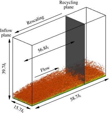
Computational domain and simulation set-up for baseline DNS case. The reference length
 $\unicode[STIX]{x1D6FF}_{i}$
is the thickness of the boundary layer (based on 99 % of the free-stream velocity) at the inlet plane. An instantaneous flow is shown in the domain, visualized by isosurface of the magnitude of density gradient,
 $|\unicode[STIX]{x1D735}\unicode[STIX]{x1D70C}|\unicode[STIX]{x1D6FF}_{i}/\unicode[STIX]{x1D70C}_{\infty }=0.9825$
, coloured by the streamwise velocity component (with levels from 0 to
 $U_{\infty }$
, blue to red).
 $x$
,
 $y$
and
 $z$
are, respectively, the streamwise, spanwise and wall-normal coordinates.

2.2 Computational domain and simulation set-up
Figure 1 shows a general computational set-up for the DNS in the present work, which parallels the set-up in Duan et al. (Reference Duan, Choudhari and Wu2014) for the Mach 2.5 simulation, wherein the effects of domain size and grid resolution were also assessed. The choice of grid parameters for the present study is based on lessons learnt from Duan et al. (Reference Duan, Choudhari and Wu2014) as summarized in table 2. The streamwise domain length (
 $L_{x}$
) is selected to be larger than the eddy decorrelation distance to guarantee minimal spurious correlation being introduced due to the inflow turbulence generation. The spanwise domain (
 $L_{y}$
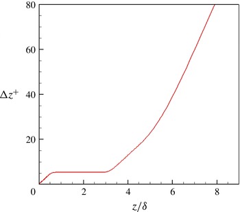
) is chosen based on monitoring the decay in cross-correlation of pressure fluctuation as a function of spanwise separation. Uniform grid spacings are used in the streamwise and spanwise directions with grid spacings. The grids in the wall-normal direction are clustered in the boundary layer with
 $\unicode[STIX]{x0394}z^{+}\approx 0.5$
at the wall, and kept uniform with
 $\unicode[STIX]{x0394}z^{+}\approx 5$
in the free stream until up to approximately
 $5.5\unicode[STIX]{x1D6FF}_{i}$
or
 $3.2\unicode[STIX]{x1D6FF}$
(figure 2), where
 $\unicode[STIX]{x1D6FF}_{i}$
and
 $\unicode[STIX]{x1D6FF}$
represent the mean boundary-layer thickness based on
 $u/U_{\infty }=0.99$
at the inflow boundary and at the downstream location selected for statistical analysis (
 $x_{a}=54.1\unicode[STIX]{x1D6FF}_{i}$
), respectively. Such wall-normal grids are designed to adequately resolve both the boundary layer and the near field of acoustic fluctuations radiated by the boundary layer. The ‘
 $+$
’ superscript denotes non-dimensionalization by the viscous length scale
 $z_{\unicode[STIX]{x1D70F}}=\unicode[STIX]{x1D708}_{w}/u_{\unicode[STIX]{x1D70F}}$
, where
 $\unicode[STIX]{x1D708}_{w}$
is the kinematic viscosity at the wall and
 $u_{\unicode[STIX]{x1D70F}}=\sqrt{\unicode[STIX]{x1D70F}_{w}/\unicode[STIX]{x1D70C}_{w}}$
is the friction velocity (
 $\unicode[STIX]{x1D70F}_{w}$
is the wall-shear stress and
 $\unicode[STIX]{x1D70C}_{w}$
is the density at the wall). Unless otherwise stated, the grid resolutions given in this section are normalized by the viscous length scale
 $z_{\unicode[STIX]{x1D70F}}$
at the selected downstream location
 $x_{a}$
. Analysis of the simulation database has also shown that the Kolmogorov length scale at
 $x_{a}$
is comparable to the local viscous length.
The wall-normal grid distribution. The grid spacing
 $\unicode[STIX]{x0394}z^{+}$
is normalized by the viscous length scale at the selected downstream location for statistical analysis (
 $x_{a}=54.1\unicode[STIX]{x1D6FF}_{i}$
).

Grid resolution and domain size for the direct numerical simulation.
 $L_{x}$
,
 $L_{y}$
and
 $L_{z}$
are the domain size in the streamwise, spanwise and wall-normal directions, respectively.
 $\unicode[STIX]{x0394}x^{+}$
and
 $\unicode[STIX]{x0394}y^{+}$
are the uniform grid spacing in the streamwise and spanwise directions, respectively.
 $\unicode[STIX]{x0394}z_{min}^{+}$
and
 $\unicode[STIX]{x0394}z_{max}^{+}$
are the minimum and maximum wall-normal grid spacing for
 $0\leqslant z/\unicode[STIX]{x1D6FF}_{i}\leqslant 5.5$
. The grid spacings are reported in terms of the viscous length scale
 $z_{\unicode[STIX]{x1D70F}}$
evaluated at the station selected for statistical analysis
 $x_{a}/\unicode[STIX]{x1D6FF}_{i}=54.1$
.
 $\unicode[STIX]{x1D6FF}_{i}=13.8~\text{mm}$
.

The turbulent inflow is generated using the recycling/rescaling method developed by Xu & Martín (Reference Xu and Martín2004) with the recycling station set at
 $56.7\unicode[STIX]{x1D6FF}_{i}$
downstream of the inlet. The selected rescaling length is similar to the range of the optimum recycling length of approximately
 $30\unicode[STIX]{x1D6FF}_{i}$
–
 $99\unicode[STIX]{x1D6FF}_{i}$
as suggested by Simens et al. (Reference Simens, Jimenez, Hoyas and Mizuno2009) to accommodate the eddy decorrelation length and to minimize inlet transients as a result of the recycling process. The original rescaling method is modified by adding the dynamic translation operations (Morgan et al.
Reference Morgan, Larsson, Kawai and Lele2011) to improve low-frequency characteristics of the generated inflow turbulence and by including a free-stream filter to remove artificial free-stream acoustics at the inlet of the computational domain introduced due to the coupling between the recycling and inflow plane (Duan et al.
Reference Duan, Choudhari and Wu2014). This removal of recycled fluctuations in the free stream ensures that the free-stream acoustic disturbances within the domain are radiated entirely from the boundary-layer turbulence rather than convected downstream from the artificial inflow. In addition, numerical experiments have been conducted with varying filter type and filtering location to ensure that the free-stream filtering has negligible effects on the pressure statistics at the selected downstream location for statistical analysis (
 $x_{a}=54.1\unicode[STIX]{x1D6FF}_{i}$
).
On the wall, no-slip conditions are applied for the three velocity components and an isothermal condition is used for the temperature with
 $T_{w}\approx 0.76T_{r}$
. The density is computed from the continuity equation. At the top and outlet boundaries, unsteady non-reflecting boundary conditions based on Thompson (Reference Thompson1987) are imposed. Periodic boundary conditions are used in the spanwise direction.
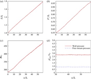
For the current spatial simulations, the boundary layer grows slowly in the streamwise direction, with both the boundary-layer thickness
 $\unicode[STIX]{x1D6FF}$
and the displacement thickness
 $\unicode[STIX]{x1D6FF}^{\ast }$
increasing by a factor of approximately two across the length of the simulation domain (figure 3). Correspondingly, the Karman number
 $Re_{\unicode[STIX]{x1D70F}}$
increases from approximately 200 at the inlet to 500 at the outlet, with a useful range of
 $Re_{\unicode[STIX]{x1D70F}}=350{-}460$
where the boundary layer has recovered from the initial transient due to the recycling method. The streamwise computational domain is large enough for the memory of the inflow generation to fade out and a nearly uniform acoustic radiation field to be established. In particular, figure 3(d) shows that the pressure fluctuations at the wall and in the free stream have become nearly homogeneous in the streamwise direction after
 $x/\unicode[STIX]{x1D6FF}_{i}\approx 30$
.
Evolution of boundary-layer parameters with streamwise distance. (a)
 $\unicode[STIX]{x1D6FF}/\unicode[STIX]{x1D6FF}_{i}$
; (b)
 $\unicode[STIX]{x1D6FF}^{\ast }/\unicode[STIX]{x1D6FF}_{i}$
; (c)
 $Re_{\unicode[STIX]{x1D70F}}$
; (d)
 $p_{rms}^{\prime }/\unicode[STIX]{x1D70F}_{w}$
at
 $z/\unicode[STIX]{x1D6FF}_{i}=0$
and 4.5.

In the following section, averages are first calculated over a streamwise window of
 $[x_{a}-0.9\unicode[STIX]{x1D6FF}_{i},x_{a}+0.9\unicode[STIX]{x1D6FF}_{i}]$
(
 $x_{a}=54.1\unicode[STIX]{x1D6FF}_{i}$
) and spanwise locations for each instantaneous flow field; then, an ensemble average over 153 flow-field snapshots spanning a time interval of approximately
 $240\unicode[STIX]{x1D6FF}_{i}/U_{\infty }$
(corresponding to
 $12.5\unicode[STIX]{x1D6FF}_{i}/u_{\unicode[STIX]{x1D70F}}$
) is calculated. To monitor the statistical convergence, flow statistics are computed by averaging over the whole or half the number of the flow-field snapshots, and a negligible difference (
 ${<}1\,\%$
) is observed between the two.
Power spectra are calculated using the Welch method (Welch Reference Welch1967) with eight segments and 50 % overlap. A Hamming window is used for weighting the data prior to the fast Fourier transform (FFT) processing. The sampling frequency is approximately
 $63U_{\infty }/\unicode[STIX]{x1D6FF}_{i}$
, or 4 MHz, and the length of an individual segment is approximately
 $53.2\unicode[STIX]{x1D6FF}_{i}/U_{\infty }$
.
2.3 Validation of DNS data
2.3.1 Velocity statistics
The velocity statistics (including the mean and root mean square (r.m.s.) values) are reported in this section at a selected downstream location for statistical analysis (
 $x_{a}=54.1\unicode[STIX]{x1D6FF}_{i}$
), which are also used in the analysis of fluctuating pressure field in § 3. Table 3 lists the values of the mean boundary-layer parameters at the selected location, including the momentum thickness
 $\unicode[STIX]{x1D703}$
and shape factor
 $H=\unicode[STIX]{x1D6FF}^{\ast }/\unicode[STIX]{x1D703}$
(where
 $\unicode[STIX]{x1D6FF}^{\ast }$
denotes the local displacement thickness). The outer and inner length scales (boundary-layer thickness
 $\unicode[STIX]{x1D6FF}$
and viscous length scale
 $z_{\unicode[STIX]{x1D70F}}$
, respectively) and the velocity scales
 $u_{\unicode[STIX]{x1D70F}}$
and
 $u_{\unicode[STIX]{x1D70F}}\sqrt{\unicode[STIX]{x1D70C}_{w}/\unicode[STIX]{x1D70C}_{\infty }}$
are also shown along with the representative Reynolds number parameters,
 $Re_{\unicode[STIX]{x1D703}}\equiv \unicode[STIX]{x1D70C}_{\infty }U_{\infty }\unicode[STIX]{x1D703}/\unicode[STIX]{x1D707}_{\infty }$
,
 $Re_{\unicode[STIX]{x1D70F}}\equiv \unicode[STIX]{x1D70C}_{w}u_{\unicode[STIX]{x1D70F}}\unicode[STIX]{x1D6FF}/\unicode[STIX]{x1D707}_{w}$
, and
 $Re_{\unicode[STIX]{x1D6FF}2}\equiv \unicode[STIX]{x1D70C}_{\infty }U_{\infty }\unicode[STIX]{x1D703}/\unicode[STIX]{x1D707}_{w}$
. Throughout this paper, the subscripts
 $\infty$
and
 $w$
are used to denote quantities at the boundary-layer edge and at the wall, respectively.
Boundary layer properties at the station selected for the analysis (
 $x_{a}=54.1\unicode[STIX]{x1D6FF}_{i}$
) of the acoustic field for the present DNS. The local boundary layer thickness
 $\unicode[STIX]{x1D6FF}$
is approximately
 $\unicode[STIX]{x1D6FF}\approx 1.7\unicode[STIX]{x1D6FF}_{i}$
.

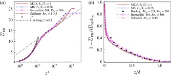
The van Driest transformed mean-velocity profile based on the DNS is shown in figure 4.
 $\bar{U}_{VD}$
is defined as
 $$\begin{eqnarray}\bar{U}_{VD}=\frac{1}{u_{\unicode[STIX]{x1D70F}}}\int _{0}^{U}(\overline{T_{w}}/\overline{T})^{1/2}\,\text{d}U.\end{eqnarray}$$
The mean velocity conforms well to the incompressible law of the wall upon van Driest transformation and shows a (narrow) logarithmic region that is comparable in extent to Mach 4 simulations by Bernardini & Pirozzoli (Reference Bernardini and Pirozzoli2011) at similar
 $Re_{\unicode[STIX]{x1D70F}}$
. In addition, the transformed mean-velocity profile compares well with the experimental results by Schlatter & Örlü (Reference Schlatter and Örlü2010) for an incompressible boundary layer at
 $Re_{\unicode[STIX]{x1D70F}}=1145$
and by Bookey et al. (Reference Bookey, Wyckham, Smits and Martin2005) at Mach 2.9,
 $Re_{\unicode[STIX]{x1D70F}}=501$
.
(a) van Driest transformed mean-velocity profile (
 $k=0.41$
,
 $C=5.2$
) and (b) van Driest transformed mean deficit velocity. Symbols denote the DNS by Bernardini & Pirozzoli (Reference Bernardini and Pirozzoli2011) at Mach 4,
 $Re_{\unicode[STIX]{x1D70F}}=506$
(circles), the experiment by Bookey et al. (Reference Bookey, Wyckham, Smits and Martin2005) at Mach 2.9,
 $Re_{\unicode[STIX]{x1D70F}}=501$
(diamonds), and the experiment by Schlatter & Örlü (Reference Schlatter and Örlü2010) for an incompressible boundary layer at
 $Re_{\unicode[STIX]{x1D70F}}=1145$
(inverted triangles).

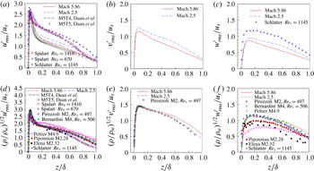
Figure 5(a–f) plots turbulence intensities and density-weighted turbulence intensities in streamwise, spanwise and wall-normal directions across the boundary layer. A significantly improved collapse of data is achieved by Morkovin’s scaling, which takes into account the variation in mean flow properties. Morkovin’s scaling brings the magnitudes of the extrema in the compressible cases closer to the incompressible results of Spalart (Reference Spalart1988) and Schlatter & Örlü (Reference Schlatter and Örlü2010), allowing the present DNS to compare well with existing data at similar conditions.
Turbulence intensities and density-weighted turbulence intensities of the (a,d) streamwise, (b,e) spanwise and (c,f) wall-normal fluctuating velocity components. —— (red): Mach 5.86,
 $M_{\infty }=5.86$
,
 $Re_{\unicode[STIX]{x1D70F}}=453.1$
,
 $T_{w}/T_{r}=0.76$
. – ⋅ – ⋅ – (blue): Mach 2.5,
 $M_{\infty }=2.5$
,
 $Re_{\unicode[STIX]{x1D70F}}=509.9$
,
 $T_{w}/T_{r}=1$
. – – –: M5T4 (Duan et al.
Reference Duan, Beekman and Martín2010),
 $M_{\infty }=5$
,
 $Re_{\unicode[STIX]{x1D70F}}=433.8$
,
 $T_{w}/T_{r}=0.68$
. ♢: M5T5 (Duan et al.
Reference Duan, Beekman and Martín2010),
 $M_{\infty }=5$
,
 $Re_{\unicode[STIX]{x1D70F}}=385.9$
,
 $T_{w}/T_{r}=1$
. ▫ (red): (Spalart Reference Spalart1988),
 $M_{\infty }\approx 0$
,
 $Re_{\unicode[STIX]{x1D703}}=1410$
. ▵ (blue): (Spalart Reference Spalart1988),
 $M_{\infty }\approx 0$
,
 $Re_{\unicode[STIX]{x1D703}}=670$
. ▿: (Pirozzoli & Bernardini Reference Pirozzoli and Bernardini2011),
 $M_{\infty }=2$
,
 $Re_{\unicode[STIX]{x1D70F}}=497$
. ● (green): (Bernardini & Pirozzoli Reference Bernardini and Pirozzoli2011),
 $M_{\infty }=4$
,
 $Re_{\unicode[STIX]{x1D70F}}=506$
. ◃ (violetred): (Peltier, Humble & Bowersox Reference Peltier, Humble and Bowersox2012),
 $M_{\infty }=4.9$
,
 $Re_{\unicode[STIX]{x1D703}}\approx 40\times 10^{3}$
,
 $T_{w}/T_{r}=0.9$
. ▪ (red): (Piponniau et al.
Reference Piponniau, Dussauge, Debieve and Dupont2009),
 $M_{\infty }=2.28$
,
 $Re_{\unicode[STIX]{x1D703}}=5100$
. ♦: (Eléna & Lacharme Reference Eléna and Lacharme1988),
 $M_{\infty }=2.32$
,
 $Re_{\unicode[STIX]{x1D703}}=4700$
. ◃ (blue): (Schlatter & Örlü Reference Schlatter and Örlü2010),
 $M_{\infty }\approx 0$
,
 $Re_{\unicode[STIX]{x1D70F}}=1145$
.

2.3.2 Comparison with experiments
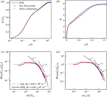
The physical realism and accuracy of the computed flow fields have been further established by comparing with existing experimental results at similar flow conditions. Figure 6 shows the comparison of DNS results (Case M6Tw076) with the wind-tunnel measurement and the calculation using Harris boundary-layer code (Harris & Blanchard Reference Harris and Blanchard1982) for a Mach
 $5.8$
turbulent boundary layer on the nozzle wall of BAM6QT under noisy-flow conditions (
 $Re=9.69\times 10^{6}~\text{m}^{-1}$
,
 $P_{t,\infty }=965~\text{kPa}$
,
 $T_{t,\infty }=429~\text{K}$
) (Steen Reference Steen2010; Casper Reference Casper2011). The DNS and experiments agree well with each other in terms of both boundary-layer profile and wall-pressure spectrum. In comparison, the Mach number profile based on the boundary-layer code exhibits larger differences from the measurement and the DNS in the outer part of the boundary layer. Moreover, figures 6(c) and 6(d) show that DNS extends the measured spectra to higher frequencies. The resolution of the high-frequency region as well as the acoustic radiation due to these high-frequency fluctuations are especially important for studying the receptivity process associated with second-mode waves in hypersonic wind tunnels.
Additional comparisons of DNS results with both experiments and other high-quality simulations are presented in the following sections.
Comparison of DNS results with those of a Mach-5.8 turbulent boundary layer on the nozzle wall of the Boeing/AFOSR Mach-6 Quiet Tunnel under noisy-flow conditions (
 $Re=9.69\times 10^{6}~\text{m}^{-1}$
,
 $P_{t,\infty }=965~\text{kPa}$
,
 $T_{t,\infty }=429~\text{K}$
). The Pitot-probe measurement of the boundary-layer profiles was conducted by Steen (Reference Steen2010); the calculation of the boundary-layer profiles using Harris boundary-layer code (Harris & Blanchard Reference Harris and Blanchard1982) and the measurement of the wall-pressure spectrum were conducted by Casper (Reference Casper2011). The experimental curve of wall-pressure spectrum is normalized with DNS-computed parameters and includes the Corcos correction for finite probe size (Beresh et al.
Reference Beresh, Henfling, Spillers and Pruett2011). (a) Mean-velocity profile; (b) Mach number profile; (c) frequency spectrum in outer scale; (d) frequency spectrum in inner scale.

3 Results
3.1 Pressure statistics
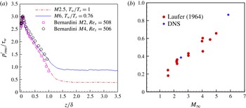
Figure 7(a) shows the r.m.s. of pressure fluctuations normalized by the local wall shear for the present DNS and some of previous DNS results at lower Mach numbers with similar Reynolds numbers (Bernardini & Pirozzoli Reference Bernardini and Pirozzoli2011; Duan et al.
Reference Duan, Choudhari and Wu2014). At the wall, the value of
 $p_{rms}^{\prime }/\unicode[STIX]{x1D70F}_{w}$
at Mach 5.86 is approximately 2.8, which is close to 3 based on the model by Bies (Reference Bies1966) and those given by the DNS of Spalart (Reference Spalart1988), Guarini et al. (Reference Guarini, Moser, Shariff and Wray2000), Bernardini & Pirozzoli (Reference Bernardini and Pirozzoli2011) at lower Mach numbers.
 $p_{rms}^{\prime }/\unicode[STIX]{x1D70F}_{w}$
is insensitive to Mach number variation within most of the boundary layer and collapses with lower Mach number data. Outside the boundary layer, however,
 $p_{rms}^{\prime }/\unicode[STIX]{x1D70F}_{w}$
approaches a constant value of approximately 0.9 for the Mach 5.86 case, which is significantly larger than the value of 0.4 for the Mach 2.5 turbulent boundary layer. The variation of free-stream pressure fluctuations with Mach number is consistent with the trend predicted by the experimental data reported by Laufer (Reference Laufer1964) (figure 7
b). Whenever all four walls of the rectangular test section were radiating to the measurement location, Laufer obtained the contribution to the acoustic fluctuations from a single wall by assuming equal contributions from each wall. This assumption was validated by comparing the measured fluctuations with those in the case where only one wall had a turbulent boundary layer and the rest had laminar boundary layers. The increase in radiation intensity with free-stream Mach number in figure 7(b) is consistent with the ‘eddy Mach wave’ hypothesis (Phillips Reference Phillips1960), which states that the ‘Mach wave type’ radiation is produced by eddies that convect supersonically with respect to the free stream. At low supersonic free-stream Mach numbers, sources that contribute primarily to the radiation field are slowly moving ones, the convection velocities of which are supersonic relative to the free stream (see figure 20). As the Mach number increases, additional faster moving turbulent eddies acquire supersonic relative speeds and start to take part in the radiation process, accounting for the larger acoustic amplitudes in the free stream.
(a) Pressure fluctuation r.m.s. profile
 $p_{rms}^{\prime }/\unicode[STIX]{x1D70F}_{w}$
as a function of wall-normal distance. The symbols denote the DNS results of Bernardini & Pirozzoli (Reference Bernardini and Pirozzoli2011). (b) Comparison of
 $p_{rms}^{\prime }/\unicode[STIX]{x1D70F}_{w}$
in the free stream with the experiments by Laufer (Reference Laufer1964), and the DNS results correspond to the present case M6Tw076 and the Mach 2.5 results of Duan et al. (Reference Duan, Choudhari and Wu2014).

3.2 Frequency spectra
The frequency spectrum of the pressure fluctuations is defined as
 $$\begin{eqnarray}\unicode[STIX]{x1D6F7}_{p}(\unicode[STIX]{x1D714})=\frac{1}{2\unicode[STIX]{x03C0}}\int _{-\infty }^{\infty }\overline{p^{\prime }(x,y,z,t)p^{\prime }(x,y,z,t+\unicode[STIX]{x1D70F})}\text{e}^{-\text{i}\unicode[STIX]{x1D714}\unicode[STIX]{x1D70F}}\,\text{d}\unicode[STIX]{x1D70F}.\end{eqnarray}$$
The pressure spectrum can be divided into several segments with different power-law scalings. According to Bull (Reference Bull1996), the pressure spectrum can be broken into regions of low, mid, mid-to-high overlap, and high frequencies, with corresponding spectrum slopes of
 $\unicode[STIX]{x1D714}^{2}$
,
 $\unicode[STIX]{x1D714}^{-1}$
,
 $\unicode[STIX]{x1D714}^{-7/3}$
, and
 $\unicode[STIX]{x1D714}^{-5}$
, respectively. The
 $\unicode[STIX]{x1D714}^{2}$
dependence of the pressure spectrum at the lowest frequencies (
 $\unicode[STIX]{x1D714}\unicode[STIX]{x1D6FF}^{\ast }/U_{\infty }<0.03$
) is induced by passive structures in the outer layer of the boundary layer. The
 $\unicode[STIX]{x1D714}^{-1}$
dependence of the pressure spectrum at mid-frequencies is typically attributed to convected turbulence in the logarithmic region where the pressure-inducing eddies has a length scale proportional to the distance from the wall (Bradshaw Reference Bradshaw1967). The
 $\unicode[STIX]{x1D714}^{-7/3}$
scaling of the pressure spectrum lies in the overlap region between mid and high frequencies and is attributed to eddies in the highest part of the buffer region (
 $20<z^{+}<30$
). Such a region is analogous to the inertial subrange in the velocity spectra that is described by Kolmogorov’s
 $-5/3$
law. The typical frequency range for this region is
 $0.3<\unicode[STIX]{x1D714}\unicode[STIX]{x1D708}/u_{\unicode[STIX]{x1D70F}}^{2}<1$
. The
 $\unicode[STIX]{x1D714}^{-5}$
dependence of the pressure spectrum at high frequencies is attributed to sources in the boundary layer below
 $z^{+}=20$
; this region is referred to as the sublayer dominance by Blake (Reference Blake1986).
Figure 8(a) shows the pressure spectrum as a function of the wall-normal distance for the present DNS. The pressure spectrum is normalized so that the area under each curve is equal to unity. For reference, straight lines with slopes of 2,
 $-1$
,
 $-7/3$
, and
 $-5$
are also included to gauge the rate of spectral roll-off across relatively low, mid, overlap, and high frequencies, respectively. The vertical lines in the plots (
 $\unicode[STIX]{x1D714}\unicode[STIX]{x1D708}_{w}/u_{\unicode[STIX]{x1D70F}}^{2}=0.3$
and
 $\unicode[STIX]{x1D714}\unicode[STIX]{x1D708}_{w}/u_{\unicode[STIX]{x1D70F}}^{2}=1.0$
) demarcate the overlap regions between mid and high frequencies and show the estimated locations where a slope change in pressure spectrum is predicted according to the theory by Bull (Reference Bull1996).
(a) Normalized frequency spectrum of computed pressure signal at selected heights for the Mach 5.86 case; (b,c) comparison of pressure spectrum at the wall and in the free stream, respectively, between the Mach 5.86 DNS and the Mach 2.5 DNS (Duan et al.
Reference Duan, Choudhari and Wu2014). The free stream is taken at
 $z/\unicode[STIX]{x1D6FF}=2.63$
for the Mach 5.86 DNS and
 $z/\unicode[STIX]{x1D6FF}=2.8$
for the Mach 2.5.

The pressure spectrum shows a rather weak frequency dependence up to the lowest frequencies covered by the DNS (
 $\unicode[STIX]{x1D714}\unicode[STIX]{x1D6FF}^{\ast }/U_{\infty }\approx 0.08$
). The absence of the more rapid and incompressible
 $\unicode[STIX]{x1D714}^{2}$
scaling as
 $\unicode[STIX]{x1D714}\rightarrow 0$
at low frequencies in the wall-pressure spectrum is consistent with the measurements by Beresh et al. (Reference Beresh, Henfling, Spillers and Pruett2011), Casper (Reference Casper2011) and the DNS by Bernardini & Pirozzoli (Reference Bernardini and Pirozzoli2011) at supersonic Mach numbers. At all wall-normal locations, there is little evidence of the
 $\unicode[STIX]{x1D714}^{-1}$
region at mid-frequencies. Given that
 $\unicode[STIX]{x1D714}^{-1}$
dependence of the pressure spectrum is attributed to sources within the logarithmic region of the boundary layer, the absence of the
 $\unicode[STIX]{x1D714}^{-1}$
region is consistent with the relatively low Reynolds number (
 $Re_{\unicode[STIX]{x1D70F}}\approx 500$
) as well as the small logarithmic region of the current DNS. In the overlap region between the mid and high frequencies, the pressure spectrum deviates from Kolmogorov’s
 $-7/3$
scaling and shows a slope of
 $\unicode[STIX]{x1D714}^{-1.6}$
at the wall. As the location of interest moves away from the wall, the deviation from the Kolmogorov scaling becomes smaller. The deviation from the Kolmogorov scaling is expected given the non-zero shear rate within the boundary layer. As a result, local isotropy cannot be realized for the current Reynolds number (Tsuji et al.
Reference Tsuji, Fransson, Alferdsson and Johansson2007). The reduced deviation from the Kolmogorov’s
 $-7/3$
scaling away from the surface can be attributed to the progressive reduction in the local shear rate. The relation between the
 $\unicode[STIX]{x1D714}^{-7/3}$
scaling of the pressure spectrum and the shear rate has previously been explained by Bernardini, Pirozzoli & Grasso (Reference Bernardini, Pirozzoli and Grasso2011), who observed the
 $\unicode[STIX]{x1D714}^{-7/3}$
behaviour of wall-pressure spectrum in a supersonic turbulent boundary layer with adverse pressure gradient and showed that such a scaling is related to a reduction of the shear rate induced by an adverse pressure gradient. At high frequencies, the spectrum exhibits a slightly more rapid decay than the
 $\unicode[STIX]{x1D714}^{-5}$
scaling predicted theoretically by Blake (Reference Blake1986), and the energy content becomes progressively lower as the location of interest moves away from the wall.
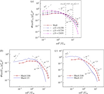
Premultiplied power spectrum of pressure signals. (a) At selected heights for the Mach 5.86 DNS; (b) comparison between Mach 5.86 and Mach 2.5 Duan et al. (Reference Duan, Choudhari and Wu2014). The pressure spectrum is normalized so that the area under each curve is equal to unity. The free stream is taken at
 $z/\unicode[STIX]{x1D6FF}=2.63$
for the Mach 5.86 DNS and
 $z/\unicode[STIX]{x1D6FF}=2.8$
for the Mach 2.5.

Figures 8(b) and 8(c) show a comparison of the pressure spectrum at the wall and in the free stream, respectively, for the present DNS at Mach 5.86 and that of a Mach 2.5 turbulent boundary layer (Duan et al.
Reference Duan, Choudhari and Wu2014). The higher Mach number case exhibits significantly higher energy than the lower Mach number case at high frequencies. A similar dependence of pressure spectrum on Mach number was shown in the experiments by Laufer (Reference Laufer1964). While an observable region of slope close to
 $-7/3$
is absent in the free-stream pressure spectrum of the Mach 5.86 DNS, the free-stream spectrum for the Mach 2.5 case has an observable region of slope close to
 $-7/3$
, indicating a possible influence of Mach number on the overlap region of the pressure spectrum. A similar Mach-number dependence of the free-stream pressure spectrum has been observed by Masutti et al. (Reference Masutti, Chazot and Carbonaro2012).
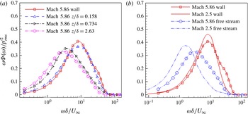
To illustrate the distribution of energy among various frequencies, figure 9(a) shows the premultiplied pressure spectra at selected heights above the surface. It is shown that the pressure spectra in the inner layer have a dominant hump centred on
 $\unicode[STIX]{x1D714}\unicode[STIX]{x1D6FF}/U_{\infty }\approx 8$
(or
 $f\unicode[STIX]{x1D6FF}/U_{\infty }\approx 1$
), which is the characteristic frequency of the energetic vortical structures within the boundary layer. As one moves away from the wall into the outer layer, the peak gradually shifts to lower frequencies as spatial intermittency becomes more important. In the free stream, where the pressure signal is predominantly acoustic, the peak of the spectrum is centred at a frequency of
 $\unicode[STIX]{x1D714}\unicode[STIX]{x1D6FF}/U_{\infty }\approx 3$
(i.e.
 $f\approx 10.8~\text{kHz}$
), indicating that characteristic frequency of the acoustic fluctuations is significantly lower than that of the vorticity mode. Similar variation in premultiplied pressure spectrum with wall-normal distance is observed for the Mach 2.5 case. Figure 9(b) further compares the premultiplied spectra for the two Mach number cases at the wall and in the free stream. While the wall spectrum is centred on nearly the same frequency
 $\unicode[STIX]{x1D714}\unicode[STIX]{x1D6FF}/U_{\infty }\approx 8$
at both Mach numbers, the free-stream spectrum for the Mach 5.86 case peaks at a significantly higher frequency than the Mach 2.5 case. The reduced gap in the dominant frequency between pressure signals at the wall and in the free stream can be explained by the ‘eddy Mach wave radiation’ concept (Phillips Reference Phillips1960; Ffowcs-Williams & Maidanik Reference Ffowcs-Williams and Maidanik1965). As the Mach number increases, additional faster-moving turbulent eddies acquire supersonic relative speeds and start in the radiation process. The increased fraction of the inner layer that can radiate to the free stream contributes to a reduced gap between the peak frequency of fluctuations near the surface and in the free stream.
3.3 Two-point correlations
3.3.1 Two-point correlations in streamwise–spanwise planes
The two-point correlation coefficient of the pressure field in a streamwise–spanwise plane is defined as
 $$\begin{eqnarray}C_{pp}(\unicode[STIX]{x0394}x,\unicode[STIX]{x0394}y,z)=\frac{\overline{p^{\prime }(x,y,z,t)p^{\prime }(x+\unicode[STIX]{x0394}x,y+\unicode[STIX]{x0394}y,z,t)}}{\left(\overline{{p^{\prime }}^{2}(x,y,z,t)}\right)^{1/2}\left(\overline{{p^{\prime }}^{2}(x+\unicode[STIX]{x0394}x,y+\unicode[STIX]{x0394}y,z,t)}\right)^{1/2}},\end{eqnarray}$$
where
 $\unicode[STIX]{x0394}x$
and
 $\unicode[STIX]{x0394}y$
are spatial separations in the streamwise and spanwise directions, respectively.
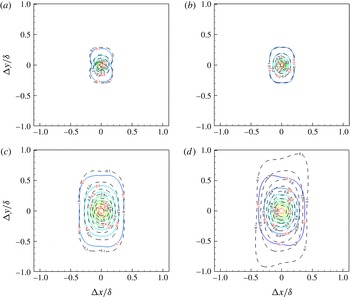
Figure 10 displays the contours of streamwise–spanwise correlation
 $C_{pp}(\unicode[STIX]{x0394}x,\unicode[STIX]{x0394}y,z)$
of the pressure fluctuations across a range of wall-normal heights for the present DNS and the Mach 2.5 case of Duan et al. (Reference Duan, Choudhari and Wu2014). The contours of
 $C_{pp}$
are approximately circular for small spatial separations but become elongated in the spanwise direction for large separation distances, indicating that the small-scale pressure-carrying eddies or wavepackets are nearly isotropic while the large-scale eddies become more coherent in the spanwise direction. The extent of the pressure contours increases in both in-plane directions as the wall-normal height increases. The two-point correlations of the pressure fluctuations in the free stream show similar patterns to those within the boundary layer, except for a variation in spatial length scales. Within the boundary layer, the pressure contours exhibit a minor Mach number dependence when non-dimensionalized by the boundary-layer thickness. In the free stream, however, the large-scale pressure wavepackets for the Mach 5.86 case become less elongated in the spanwise direction compared with the lower Mach number case.
Contours of constant streamwise–spanwise correlation coefficient of the pressure signal
 $C_{pp}(\unicode[STIX]{x0394}x,\unicode[STIX]{x0394}y)$
at selected heights for Mach 5.86 (coloured solid line) and Mach 2.5 (black dashed line). Contour levels vary from 0.1 to 0.9 with increments of 0.1. (a) Wall, (b)
 $z/\unicode[STIX]{x1D6FF}=0.158$
, (c)
 $z/\unicode[STIX]{x1D6FF}=0.734$
, (d)
 $z/\unicode[STIX]{x1D6FF}=2.631$
.

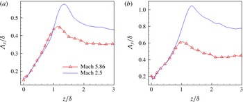
Figures 11(a) and 11(b) show the variation of streamwise and spanwise length scales of the pressure field (
 $(\unicode[STIX]{x1D6EC}_{x})_{p}$
and
 $(\unicode[STIX]{x1D6EC}_{y})_{p}$
), respectively, as a function of wall-normal distance.
(a) Streamwise
 $\unicode[STIX]{x1D6EC}_{x}$
and (b) spanwise
 $\unicode[STIX]{x1D6EC}_{y}$
integral length scales as a function of the wall-normal location.
 $\unicode[STIX]{x1D6EC}_{x}\equiv \int C_{pp}(\unicode[STIX]{x0394}x,0,0)\,\text{d}(\unicode[STIX]{x0394}x)$
and
 $\unicode[STIX]{x1D6EC}_{y}\equiv \int C_{pp}(0,\unicode[STIX]{x0394}y,0)\text{d}(\unicode[STIX]{x0394}y)$
, with the limits of the integral chosen as the streamwise and spanwise separations between the two crossings of
 $C_{pp}=0.1$
.

The streamwise and spanwise length scales of the pressure field display an approximate increase with wall-normal coordinate within most of the boundary layer, reaching a peak just outside the boundary-layer edge. For approximately
 $z/\unicode[STIX]{x1D6FF}>2$
, both scales again relax to approximately constant values that are nearly twenty-five percent lower than the respective peaks. Such a dependence of length scales on the wall-normal coordinate is consistent with wall-normal variation of the extent of pressure correlation contours shown in figure 10. The nearly linear increase of pressure length scales with wall-normal location in the outer region of the boundary layer is consistent with the conceptual model of very large-scale motion (VLSM) proposed by Kim & Adrian (Reference Kim and Adrian1999). Similar wall-normal variation of large-scale coherence has been revealed by particle image velocimetry (PIV) experiments of turbulent boundary layers at low and supersonic speeds (Tomkins & Adrian Reference Tomkins and Adrian2003; Ganapathisubramani et al.
Reference Ganapathisubramani, Clemens, Hambleton, Longmire and Marusic2005; Ganapathisubramani, Clemens & Dolling Reference Ganapathisubramani, Clemens and Dolling2006) based on two-point correlations of streamwise velocity fluctuations.
3.3.2 Two-point correlations in streamwise–wall-normal planes
The two-point correlation coefficient of the pressure field in a streamwise–wall-normal plane is defined as
 $$\begin{eqnarray}C_{pp}(\unicode[STIX]{x0394}x,z,z_{\mathit{ref}})=\frac{\overline{p^{\prime }(x,y,z_{\mathit{ref}},t)p^{\prime }(x+\unicode[STIX]{x0394}x,y,z,t)}}{\left(\overline{{p^{\prime }}^{2}(x,y,z_{\mathit{ref}},t)}\right)^{1/2}\left(\overline{{p^{\prime }}^{2}(x+\unicode[STIX]{x0394}x,y,z,t)}\right)^{1/2}},\end{eqnarray}$$
where
 $\unicode[STIX]{x0394}x$
is spatial separations in the streamwise direction and
 $z_{\mathit{ref}}$
is the reference wall-normal location at which the correlation is computed.
Contours of constant
 $C_{pp}(\unicode[STIX]{x0394}x,z,z_{\mathit{ref}})$
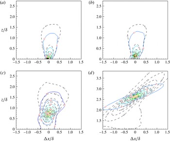
for the present Mach 5.86 DNS at multiple reference heights
 $z_{\mathit{ref}}$
are shown in figure 12. The same contours for the Mach 2.5 DNS (Duan et al.
Reference Duan, Choudhari and Wu2014) are also included to highlight the differences from the lower Mach number case. For each reference height
 $z_{\mathit{ref}}$
, the maximum correlation of pressure fluctuations is approximately aligned along a line, indicating the presence of downward-leaning structures. At the wall, the structure of pressure fluctuations is inclined approximately
 $\unicode[STIX]{x1D703}_{xz}\approx 80^{\circ }$
to the wall. The inclination angle decreases gradually in the inner and outer regions of the boundary layer. In the free stream, the inclination angle of the pressure-structure plateaus to
 $\unicode[STIX]{x1D703}_{xz}\approx 21^{\circ }$
. The variation in
 $\unicode[STIX]{x1D703}_{xz}$
with wall-normal distance indicates that pressure disturbances generated within the boundary layer will undergo significant refraction before they are radiated to the free stream. The free-stream pressure wave-front inclination
 $\unicode[STIX]{x1D703}_{xz}$
closely matches the wave-front orientation of the instantaneous acoustic radiation visualized by numerical Schlieren imaging as shown in figure 19(a).
The pressure-structure angle exhibits minor Mach number dependence within the boundary layer. In the free stream, however, the pressure wave front is significantly shallower for the higher Mach number case. The shallower wave front of the free-stream radiation for the higher Mach number case is consistent with the decrease in the zone of influence of a flow disturbance as Mach number increases.
Streamwise wall-normal correlation coefficient of the pressure signal
 $C_{pp}(\unicode[STIX]{x0394}x,z,z_{\mathit{ref}})$
at selected heights for Mach 5.86 (coloured solid line) and Mach 2.5 (black dashed line). Contour levels vary from 0.1 to 0.9 with increments of 0.1. (a)
 $z_{ref}/\unicode[STIX]{x1D6FF}=0$
, (b)
 $z_{ref}/\unicode[STIX]{x1D6FF}=0.158$
, (c)
 $z_{ref}/\unicode[STIX]{x1D6FF}=0.734$
, (d)
 $z_{ref}/\unicode[STIX]{x1D6FF}=2.631$
.

3.3.3 Space–time correlation
The space–time of the pressure field is defined as
 $$\begin{eqnarray}C_{pp}(\unicode[STIX]{x0394}x,\unicode[STIX]{x0394}t)=\frac{\overline{p^{\prime }(x,y,z,t)p^{\prime }(x+\unicode[STIX]{x0394}x,y,z,t+\unicode[STIX]{x0394}t)}}{\left(\overline{{p^{\prime }}^{2}(x,y,z,t)}\right)^{1/2}\left(\overline{{p^{\prime }}^{2}(x+\unicode[STIX]{x0394}x,y,z,t+\unicode[STIX]{x0394}t)}\right)^{1/2}},\end{eqnarray}$$
where
 $\unicode[STIX]{x0394}x$
and
 $\unicode[STIX]{x0394}t$
are spatial separation in the streamwise direction and the time delay, respectively.
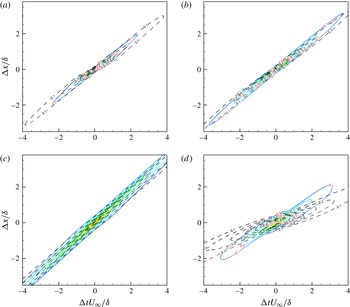
The space–time correlation contours of
 $C_{pp}(\unicode[STIX]{x0394}x,\unicode[STIX]{x0394}t)$
are plotted at multiple wall-normal locations as shown in figure 13. For comparison, the same contours for the Mach 2.5 DNS (Duan et al.
Reference Duan, Choudhari and Wu2014) are also included. At all wall-normal locations, the pressure contours are skewed, with the maximum correlation aligned along the first or third quadrant in the (
 $\unicode[STIX]{x0394}x$
,
 $\unicode[STIX]{x0394}t$
)-plane. The concentration of contours of
 $C_{pp}(\unicode[STIX]{x0394}x,\unicode[STIX]{x0394}t)$
into a narrow band indicates strong downstream propagation of pressure fluctuations. In addition, there is a change in the overall slope of
 $\text{d}\unicode[STIX]{x0394}x/\text{d}\unicode[STIX]{x0394}t$
at different wall-normal locations, indicating a variation of bulk propagation speed of pressure fluctuations as a function of wall-normal distance. The overall larger inclination of the space–time correlation contours in the free stream for the Mach 5.86 case indicates that the free-stream pressure structures propagate with a larger speed relative to the Mach 2.5 case. A further discussion of the propagation speed of pressure fluctuations, including its dependence on different definitions, will be given in § 3.4.
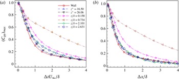
Figures 14(a) and 14(b) plot the maximum space–time correlation of pressure fluctuations,
 $(C_{pp})_{max}$
, as a function of time delay
 $\unicode[STIX]{x0394}t$
and streamwise separation
 $\unicode[STIX]{x0394}x$
, respectively, at multiple wall-normal locations. The scales of temporal and spatial decays in
 $(C_{pp})_{max}$
are measures of the lifetime and Lagrangian decorrelation length of the coherent pressure structures or wavepackets. Within the boundary layer, the temporal and spatial Lagrangian scales of the pressure structures increase with wall-normal distance and are at least five times larger than the large-eddy turnover time and the boundary-layer thickness, respectively. In the free stream, the acoustic pressure fluctuations show similar temporal and spatial decay rates as those near the wall (
 $z^{+}\approx 20$
). Given that acoustic sources are concentrated in the near-wall region according to the concept of ‘eddy Mach wave radiation’ (§ 4.3), the apparent match in the Lagrangian time and spatial scales between the free-stream pressure structures and the structures near the wall indicates that the free-stream acoustic radiation mainly originates from the near-wall region, a finding that is consistent with the concept of ‘eddy Mach waves’.
Contours of constant space–time correlation coefficient of pressure fluctuations
 $C_{pp}(\unicode[STIX]{x0394}x,\unicode[STIX]{x0394}t)$
at selected heights for Mach 5.86 (coloured solid line) and Mach 2.5 (black dashed line). Contour levels vary from 0.1 to 0.9 with increments of 0.1. (a) Wall, (b)
 $z/\unicode[STIX]{x1D6FF}=0.158$
, (c)
 $z/\unicode[STIX]{x1D6FF}=0.734$
, (d)
 $z/\unicode[STIX]{x1D6FF}=2.631$
.

Decay of the maximum spatial–time correlation coefficient of pressure fluctuations,
 $(C_{pp})_{max}$
, as a function of (a) time delay
 $\unicode[STIX]{x0394}t$
and (b) streamwise separation
 $\unicode[STIX]{x0394}x$
.

3.4 Propagation speed
The space–time correlation data based on the DNS was used to estimate the speed of propagation of pressure fluctuations. First, for a given time delay
 $\unicode[STIX]{x0394}t$
, the propagation speed
 $U_{c}$
is defined as the ratio
 $\unicode[STIX]{x0394}x/\unicode[STIX]{x0394}t$
at the value of
 $\unicode[STIX]{x0394}x$
where
 $$\begin{eqnarray}\left.\frac{\unicode[STIX]{x2202}C_{pp}(r_{x},0,\unicode[STIX]{x0394}t)}{\unicode[STIX]{x2202}r_{x}}\right|_{r_{x}=\unicode[STIX]{x0394}x}=0.\end{eqnarray}$$
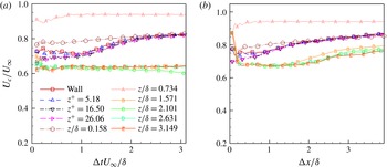
A similar procedure has been used by multiple researchers (Kim Reference Kim1989; Choi & Moin Reference Choi and Moin1990; Bernardini & Pirozzoli Reference Bernardini and Pirozzoli2011) to define the convection speed of wall-pressure fluctuations. Figure 15(a) plots the propagation speed as a function of time delay
 $\unicode[STIX]{x0394}t$
at several selected heights across the boundary layer for the present DNS. As expected, the propagation speed shows a
 $\unicode[STIX]{x0394}t$
dependence, and there is an increase in
 $U_{c}$
at large time separations in the inner and outer layers of the boundary layer (
 $z/\unicode[STIX]{x1D6FF}<1$
). Given that only large eddies retain their coherence at large time separations, such an increase in
 $U_{c}$
at large
 $\unicode[STIX]{x0394}t$
may suggest that large pressure-carrying eddies/wavepackets propagate with higher speeds than small ones. The propagation speed at the wall is
 $U_{c}\approx 0.8U_{\infty }$
for the large-scale disturbances (associated with large time delay) and
 $U_{c}\approx 0.72U_{\infty }$
for the small-scale disturbances (associated with small time delay). The magnitude of the propagation speed near the surface as well as its scale dependence is in close agreement with both measured and computed values for low-speed and supersonic turbulent boundary-layer flows (Willmarth Reference Willmarth1975; Choi & Moin Reference Choi and Moin1990; Tsuji et al.
Reference Tsuji, Fransson, Alferdsson and Johansson2007; Bernardini & Pirozzoli Reference Bernardini and Pirozzoli2011). The propagation velocity becomes less scale dependent in the log layer (
 $z/\unicode[STIX]{x1D6FF}=0.16$
) and the outer layer (
 $z/\unicode[STIX]{x1D6FF}=0.73$
), and the overall range is very close to the local mean velocity. Outside the boundary layer, the propagation speed is again insensitive to
 $\unicode[STIX]{x0394}t$
and the pressure wavepackets propagate at a significantly smaller speed of
 $U_{c}\approx 0.63U_{\infty }$
. Similar findings were reported by Duan et al. (Reference Duan, Choudhari and Wu2014) for a Mach 2.5 turbulent boundary layer. The significantly smaller propagation speed of the free-stream pressure wavepackets indicates that the acoustic sources that radiate noise into the free stream convect with a speed much smaller than the free-stream velocity.
Propagation speed of pressure fluctuations as a function of (a) time delay
 $\unicode[STIX]{x0394}t$
and (b) streamwise separation
 $\unicode[STIX]{x0394}x$
for the DNS of Mach 5.86 turbulent boundary layer.

As suggested by Laufer (Reference Laufer1964), the propagation speed
 $U_{c}\equiv \unicode[STIX]{x0394}x/\unicode[STIX]{x0394}t$
can also be defined for a given
 $\unicode[STIX]{x0394}x$
and at the value of
 $\unicode[STIX]{x0394}t$
where
 $$\begin{eqnarray}\left.\frac{\unicode[STIX]{x2202}C(\unicode[STIX]{x0394}x,0,r_{t})}{\unicode[STIX]{x2202}r_{t}}\right|_{r_{t}=\unicode[STIX]{x0394}t}=0.\end{eqnarray}$$
This definition is consistent with Laufer’s experiments (Laufer Reference Laufer1964) in which two probes with fixed streamwise separation are used to determine the propagation speed. Figure 15(b) shows a plot of the propagation speed
 $U_{c}$
as a function of streamwise separation
 $\unicode[STIX]{x0394}x$
at selected wall-normal locations. Similar to figure 15(a), the propagation speed in the inner layer increases at large streamwise separations, and such an increase becomes less significant as the location of interest moves to the outer layer. In the free stream,
 $U_{c}/U_{\infty }$
is approximately 0.68 for
 $\unicode[STIX]{x0394}x/\unicode[STIX]{x1D6FF}\approx 0.23$
(corresponding to the probe separation
 $\unicode[STIX]{x0394}x_{\mathit{Laufer}}=0.71$
centimetres in Laufer’s experiment by assuming
 $\unicode[STIX]{x1D6FF}_{\mathit{Laufer}}=3.15~\text{cm}$
).
A third way to quantify the overall propagation speed of pressure-carrying eddies or wavepackets is to find the value of
 $U_{b}$
which minimizes the difference between the real time evolution of
 $p(x,t)$
and a frozen wave
 $p(x-U_{b}t)$
. Following this definition, the following expression can be obtained
 $$\begin{eqnarray}U_{b}\equiv -\frac{\overline{(\unicode[STIX]{x2202}p/\unicode[STIX]{x2202}t)(\unicode[STIX]{x2202}p/\unicode[STIX]{x2202}x)}}{\overline{(\unicode[STIX]{x2202}p/\unicode[STIX]{x2202}x)^{2}}}.\end{eqnarray}$$
The same definition of bulk propagation speed was introduced by Del Alamo & Jimenez (Reference Del Alamo and Jimenez2009) for the streamwise velocity fluctuations. Similar to the streamwise velocity (Del Alamo & Jimenez Reference Del Alamo and Jimenez2009), a figure of merit for the frozen-wave approximation can be introduced for the pressure fluctuations as
 $$\begin{eqnarray}\unicode[STIX]{x1D6FE}_{p}\equiv \frac{\left|\overline{(\unicode[STIX]{x2202}p/\unicode[STIX]{x2202}x)(\unicode[STIX]{x2202}p/\unicode[STIX]{x2202}t)}\right|}{\left[\overline{\left(\unicode[STIX]{x2202}p/\unicode[STIX]{x2202}t\right)^{2}}\;\overline{\left(\unicode[STIX]{x2202}p/\unicode[STIX]{x2202}x\right)^{2}}\right]^{1/2}}.\end{eqnarray}$$
 $\unicode[STIX]{x1D6FE}_{p}$
equals unity for a perfect frozen wave, and zero for fast decaying or deforming waves as they convect downstream.
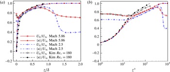
Figure 16 plots the bulk propagation speed of the pressure fluctuation as a function of wall-normal distance. The bulk propagation speed of the pressure fluctuation is significantly larger than the local mean velocity in the viscous sublayer and the buffer layer. The bulk propagation speed of the pressure fluctuation becomes approximately equal to the local mean velocity in the upper buffer layer and remains so over a significant portion of the boundary layer (up to
 $z/\unicode[STIX]{x1D6FF}\approx 0.65$
). Such a variation of
 $U_{b}$
within the boundary layer is consistent with the findings for incompressible and lower Mach number supersonic flows (Kim & Hussain Reference Kim and Hussain1993; Duan et al.
Reference Duan, Choudhari and Wu2014). In the free stream, the propagation speed departs from Taylor’s hypothesis and is significantly lower than the local mean velocity. Figure 17 shows the wall-normal distribution of the correlation coefficient
 $\unicode[STIX]{x1D6FE}_{p}$
that provides a figure of merit for the frozen-wave approximation. The pressure wave is nearly frozen with
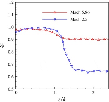
 $\unicode[STIX]{x1D6FE}\approx 1$
within the boundary layer and becomes less so outside the boundary layer at both Mach numbers. As the Mach number increases, propagation effects become significantly more dominant over evolution effects for the free-stream pressure wave.
Wall-normal distribution of bulk propagation speed of pressure fluctuations in (a) outer and (b) inner units.
 $U_{b}$
is defined based on ‘frozen-wave’ approximation as (3.7) (Del Alamo & Jimenez Reference Del Alamo and Jimenez2009) for the Mach 5.86 and Mach 2.5 DNS, and is calculated using (3.5) with
 $\unicode[STIX]{x0394}t^{+}=18$
for the incompressible DNS by Kim & Hussain (Reference Kim and Hussain1993).

The distribution of correlation coefficient
 $\unicode[STIX]{x1D6FE}_{p}=|\overline{(\unicode[STIX]{x2202}p/\unicode[STIX]{x2202}x)(\unicode[STIX]{x2202}p/\unicode[STIX]{x2202}t)}|/[\overline{(\unicode[STIX]{x2202}p/\unicode[STIX]{x2202}t)^{2}}\;\overline{(\unicode[STIX]{x2202}p/\unicode[STIX]{x2202}x)^{2}}]^{1/2}$
that provides a figure of merit for the frozen-wave approximation.

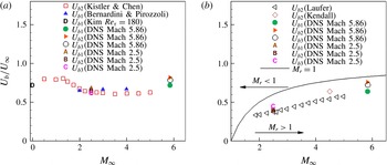
Figure 18 compares the bulk propagation speed at the wall and in the free stream with some existing experiments and simulations. In the figure,
 $U_{b1}$
is defined based on the space–time correlation coefficient with (3.5) for the time delay
 $\unicode[STIX]{x0394}t$
or frequency (
 $\unicode[STIX]{x1D714}=2\unicode[STIX]{x03C0}/\unicode[STIX]{x0394}t$
) where the premultiplied frequency spectrum (figure 9
a) attains its maximum. In analogy,
 $U_{b2}$
is derived based on (3.6) for the streamwise separation
 $\unicode[STIX]{x0394}x$
or wavenumber (
 $k_{1}=2\unicode[STIX]{x03C0}/\unicode[STIX]{x0394}x$
) where the premultiplied one-dimensional wavenumber spectrum attains its maximum.
 $U_{b3}$
is computed using (3.7) by assuming ‘frozen wave/eddy’. The values of bulk propagation speed
 $U_{b}$
varies depending on specific definitions. Similar findings were reported for the convection speed of the wall pressure (Choi & Moin Reference Choi and Moin1990). The value of
 $U_{b}$
at the wall gradually increases with the free-stream Mach number and is slightly higher than those widely quoted for low-speed flows (Willmarth Reference Willmarth1975; Choi & Moin Reference Choi and Moin1990; Tsuji et al.
Reference Tsuji, Fransson, Alferdsson and Johansson2007). The gradual increase in propagation speeds with Mach number is consistent with the values reported by Bernardini & Pirozzoli (Reference Bernardini and Pirozzoli2011) for turbulent boundary layers at Mach 2, 3 and 4 (figure 18
a). In the free stream, the bulk propagation speed is approximately equal to
 $0.7U_{\infty }$
. Such a free-stream propagation speed falls within the region where
 $M_{r}>1$
, with
 $M_{r}\equiv (U_{\infty }-U_{b})/a_{\infty }$
, consistent with the concept of ‘eddy Mach wave’ radiation (Phillips Reference Phillips1960; Ffowcs-Williams & Maidanik Reference Ffowcs-Williams and Maidanik1965). Figure 18(b) further shows that the DNS-computed propagation speed compares well with existing experiments and simulations (Laufer Reference Laufer1964; Duan et al.
Reference Duan, Choudhari and Wu2014).
Bulk convection speed of pressure fluctuations as a function of free-stream Mach number: (a) at the wall; (b) in the free stream. Symbols: squares: Kistler & Chen (Reference Kistler and Chen1963); up triangles: Bernardini & Pirozzoli (Reference Bernardini and Pirozzoli2011); left triangles: Laufer (Reference Laufer1964); diamonds: Kendall (Reference Kendall1970); letter D: Kim (Reference Kim1989); filled circles: DNS Mach 5.86; right triangles: DNS Mach 5.86; open circles: DNS Mach 5.86; letter A: DNS Mach 2.5 (Duan et al.
Reference Duan, Choudhari and Wu2014); letter B: DNS Mach 2.5; letter C: DNS Mach 2.5; Lines:
 $M_{r}=1$
.
 $U_{b1}:\unicode[STIX]{x2202}C(r_{x},0,\unicode[STIX]{x0394}t)/\unicode[STIX]{x2202}r_{x}|_{r_{x}=\unicode[STIX]{x0394}x}=0$
,
 $U_{b2}:\unicode[STIX]{x2202}C(\unicode[STIX]{x0394}x,0,r_{t})/\unicode[STIX]{x2202}r_{t}|_{r_{t}=\unicode[STIX]{x0394}t}=0$
.
 $U_{b3}:-\overline{(\unicode[STIX]{x2202}p/\unicode[STIX]{x2202}t)(\unicode[STIX]{x2202}p/\unicode[STIX]{x2202}x)}/\overline{(\unicode[STIX]{x2202}p/\unicode[STIX]{x2202}x)^{2}}$
.

4 Free-stream acoustic radiation
4.1 Characteristics of free-stream fluctuations
In this section, the nature of free-stream acoustic fluctuations is analysed using the present DNS data at Mach 5.86 and compared with previous results at Mach 2.5 (Duan et al. Reference Duan, Choudhari and Wu2014).
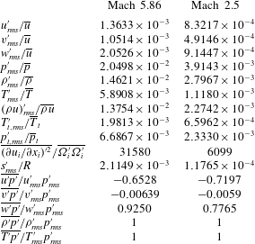
Table 4 lists the free-stream values of several fluctuating flow variables for the present DNS at Mach 5.86 and the Mach 2.5 DNS (Duan et al.
Reference Duan, Choudhari and Wu2014). Similar to the Mach 2.5 case, the free-stream thermodynamic fluctuations for the present Mach 5.86 case satisfy isentropic relations, indicating the acoustic nature of free-stream fluctuations. Moreover, the level of dilatational fluctuations
 $\overline{{(\unicode[STIX]{x2202}u_{i}/\unicode[STIX]{x2202}x_{i})^{\prime }}^{2}}$
, which is representative of the acoustic mode, is compared with the magnitude of vortical fluctuations
 $\overline{\unicode[STIX]{x1D6FA}_{i}^{\prime }\unicode[STIX]{x1D6FA}_{i}^{\prime }}$
, which is representative of vorticity mode. The large values of
 $\overline{{(\unicode[STIX]{x2202}u_{i}/\unicode[STIX]{x2202}x_{i})^{\prime }}^{2}}/\overline{\unicode[STIX]{x1D6FA}_{i}^{\prime }\unicode[STIX]{x1D6FA}_{i}^{\prime }}$
as well as the small values of entropy fluctuations
 $s_{rms}^{\prime }/R$
relative to
 $p_{rms}^{\prime }/\bar{p}$
imply that the acoustic mode is dominant over the vorticity and entropy modes in the free stream in terms of modal compositions (Kovasznay Reference Kovasznay1953). The dominance of the acoustic mode over the other two modes confirms that a purely acoustic field in the free stream is successfully isolated by the present DNS. Thus, the present simulation provides a unique opportunity for studying the similarities and differences in the characteristics of the primarily vortical fluctuations within the boundary layer and acoustic fluctuations in the free stream.
The disturbance field at
 $z/\unicode[STIX]{x1D6FF}=2.63$
for Case Mach 5.86 and
 $z/\unicode[STIX]{x1D6FF}=2.8$
for Case Mach 2.5.
 $R$
is the gas constant in the ideal-gas equation of state
 $p=\unicode[STIX]{x1D70C}RT$
.

The normalized velocity fluctuations at Mach 5.86 are significantly larger than those at Mach 2.5. Yet, the r.m.s. fluctuations in either velocity component are less than approximately 0.25 %. The fluctuations in thermodynamic variables are stronger than the velocity fluctuations and also increase from Mach 2.5 to Mach 5.86. At Mach 5.86, the r.m.s. pressure fluctuations are approximately 2 % of the mean pressure value, compared with
 $\overline{p_{rms}^{\prime }}/\bar{p}\approx 0.4\,\%$
at Mach 2.5. The increase in fluctuating intensity with the Mach number is consistent with the theory of ‘Mach wave radiation’ and the experimental findings by Laufer (Reference Laufer1964). For both Mach number cases, the pressure fluctuations are strongly correlated with the streamwise velocity (
 $u$
) and the wall-normal velocity (
 $w$
), but almost uncorrelated with the spanwise velocity (
 $v$
). The large negative value of
 $\overline{u^{\prime }p^{\prime }}$
and positive value of
 $\overline{w^{\prime }p^{\prime }}$
indicate that the free-stream radiation may be approximated by two-dimensional, backward-facing waves. The changes in values of
 $\overline{w^{\prime }p^{\prime }}/w_{rms}^{\prime }p_{rms}^{\prime }$
and
 $\overline{u^{\prime }p^{\prime }}/u_{rms}^{\prime }p_{rms}^{\prime }$
between the Mach 2.5 and Mach 5.86 cases indicate a variation of the directionality of the free-stream radiation with the Mach number (see § 4.2).
4.2 Wave-front orientation
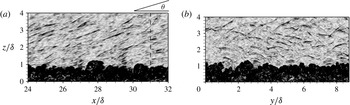
In this section, the directionality of the stochastic acoustic field in the free stream is discussed given its importance to hypersonic transition testing in conventional wind tunnels. Figure 19(a) shows that the instantaneous pressure field in the free stream consists of randomly spaced wave fronts, each with a limited spatial coherence. The wave fronts exhibit a preferred orientation within the streamwise–wall-normal (
 $x{-}z$
) plane. The orientation of the instantaneous free-stream pressure field is similar to that of the free-stream pressure structures that are defined in the statistical sense based on
 $C_{pp}(\unicode[STIX]{x0394}x,z,z_{\mathit{ref}})$
(figure 12
d) with
 $\unicode[STIX]{x1D703}\approx \unicode[STIX]{x1D703}_{xz}=21^{\circ }$
.
Numerical Schlieren image based on instantaneous flow field for the present DNS of a Mach 5.86 turbulent boundary layer. Contour levels are selected to emphasize disturbances in the free stream.
 $\unicode[STIX]{x1D703}$
is the angle between the flow direction and the acoustic wave front, and the vertical dashed line in (a) indicates the streamwise location of the selected spanwise–wall-normal plane visualized in (b).

An alternative way of defining the free-stream wave-front orientation is to assume that the two-dimensional free-stream acoustic field consists of planar acoustic waves. The wave-front orientation can therefore be derived using the following plane-acoustic-wave relation (Liepmann & Roshko Reference Liepmann and Roshko1957)
 $$\begin{eqnarray}\frac{u_{n}^{\prime }}{U_{\infty }}=\frac{1}{\unicode[STIX]{x1D6FE}M_{\infty }}\frac{p^{\prime }}{p_{\infty }},\end{eqnarray}$$
where
 $u_{n}^{\prime }=\boldsymbol{u}^{\prime }\boldsymbol{\cdot }\boldsymbol{n}=u^{\prime }\cos \unicode[STIX]{x1D703}_{n}+w^{\prime }\sin \unicode[STIX]{x1D703}_{n}$
is the velocity normal to the wave front and
 $\boldsymbol{n}=(\cos \unicode[STIX]{x1D703}_{n},\sin \unicode[STIX]{x1D703}_{n})$
is the plane-wave normal direction, with
 $\unicode[STIX]{x1D703}_{n}$
the angle between
 $\boldsymbol{u}$
and
 $\boldsymbol{n}$
. The wave-front orientation that is statistically most likely can be determined to be the direction that minimizes the difference between
 $u_{n,rms}^{\prime }/U_{\infty }$
and
 $p_{rms}^{\prime }/(\unicode[STIX]{x1D6FE}M_{\infty }p_{\infty })$
. By using the free-stream statistics analogous to table 4,
 $\unicode[STIX]{x1D703}_{n}\approx 120^{\circ }$
(correspondingly
 $\unicode[STIX]{x1D703}\approx 30^{\circ }$
) is obtained. For comparison, the wave angle of acoustic radiation for a Mach 2.5 turbulent boundary layer is
 $\unicode[STIX]{x1D703}=42^{\circ }$
(Duan et al.
Reference Duan, Choudhari and Wu2014). Laufer (Reference Laufer1964) has used a similar but less rigorous relation
 $u_{n}^{\prime }\cos \unicode[STIX]{x1D703}_{n}=u^{\prime }$
to estimate the wave orientation, since the streamwise velocity fluctuation
 $u^{\prime }$
is the only velocity component that could be measured in his experiments.
The differences in the calculated wave angles
 $\unicode[STIX]{x1D703}$
based on the plane-acoustic-wave assumption and the two-point correlation
 $C_{pp}(\unicode[STIX]{x0394}x,z,z_{\mathit{ref}})$
indicate that the free-stream acoustic field does not correspond to truly planar waves. The deviation from purely planar behaviour is also indicated by the imperfect correlation between
 $p^{\prime }$
and the streamwise (
 $u^{\prime }$
) and wall-normal (
 $w^{\prime }$
) velocity fluctuations in the free-stream region (recall the data presented in table 4). As seen from figure 19(b), a substantial portion of the instantaneous pressure field within the region of interest corresponds to conical disturbances propagating from some (possibly virtual) localized source within the boundary layer. The finite spanwise extent of the pressure wavepackets is consistent with the finite size of acoustic sources that are responsible for generating the waves. The details of the acoustic sources will be discussed in § 4.3.
4.3 Sources of free-stream acoustic radiation
In this section, the acoustic sources that give rise to the acoustic pressure fluctuations in the free stream are approximated in terms of flow turbulence according to the acoustic analogy approach by Phillips (Reference Phillips1960). The Phillips’ form of the acoustic analogy equation, the definition of acoustic source terms as well as their decomposition into linear and quadratic components are given in Duan et al. (Reference Duan, Choudhari and Wu2014).
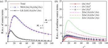
Figure 20(a) plots the root mean square (r.m.s.) of the acoustic source term including both linear and nonlinear components as functions of
 $z$
across the near-wall portion of the boundary layer. Similar to the Mach 2.5 case (Duan et al.
Reference Duan, Choudhari and Wu2014), the total source term for the present DNS peaks at
 $z^{+}\approx 20$
and the nonlinear source term is dominant over the linear source term throughout the boundary layer. Among the six constituent terms of the nonlinear acoustic source (figure 20
b),
 $(\unicode[STIX]{x2202}v^{\prime }/\unicode[STIX]{x2202}z)(\unicode[STIX]{x2202}w^{\prime }/\unicode[STIX]{x2202}y)$
has the largest r.m.s. value, with approximately the same peak location as the total acoustic source. The dominance of
 $(\unicode[STIX]{x2202}v^{\prime }/\unicode[STIX]{x2202}z)(\unicode[STIX]{x2202}w^{\prime }/\unicode[STIX]{x2202}y)$
in the buffer layer may indicate the important role played by the near-wall streamwise structures in sound generation. Similar distribution of source terms as well as the dominance of the nonlinear components have been reported by Kim (Reference Kim1989) in the context of incompressible flows.
Profiles of the r.m.s. source terms (including the total, nonlinear source (NLS), and linear source (LS) terms) across the near-wall portion of the boundary layer. The r.m.s. of the source terms are normalized by
 $(\unicode[STIX]{x1D6FF}^{2}/U_{\infty }^{2})$
.

We note that the magnitude of the source terms is not the sole determinant of the local contribution to the acoustic radiation in the free stream. The solution to the acoustic analogy equation is given by the convolution of the source terms with the Green’s function of this equation, which may be viewed as the local efficiency of the conversion of hydrodynamic source terms into radiating acoustic disturbances. Due to the dramatic differences in the ability of sound generation between turbulent sources that travel at subsonic or supersonic speeds relative to the free stream (i.e. the basic concept of ‘eddy Mach wave’ (Phillips Reference Phillips1960; Ffowcs-Williams & Maidanik Reference Ffowcs-Williams and Maidanik1965)), figure 20(a) also shows the regions of flow with a supersonic (
 $M_{r}>1$
) and subsonic (
 $M_{r}<1$
) relative Mach number. The relative sonic location (
 $M_{r}=1$
) for the Mach 5.86 lies at
 $z^{+}\approx 114$
(
 $z/\unicode[STIX]{x1D6FF}\approx 0.25$
), compared with
 $z^{+}\approx 22$
(
 $z/\unicode[STIX]{x1D6FF}\approx 0.04$
) for the Mach 2.5 case, indicating a dramatic increase in the fraction of sound-radiating eddies as the free-stream Mach number increases. The increased portion of sound-generating eddies is consistent with the enhanced radiation intensity as the free-stream Mach number increases (figure 7
b). Moreover, the increased fraction of the inner layer that can radiate to the free stream contributes to a reduced gap between the peak frequency of fluctuations near the surface and within the free stream, as shown by figure 9(b).
5 Summary and conclusions
DNS of a zero-pressure-gradient turbulent boundary layer with a nominal free-stream Mach number of 5.86 and a wall-to-recovery temperature ratio of
 $T_{w}/T_{r}=0.76$
is conducted to investigate the wall-normal variation of the fluctuating pressure field and highlight the differences between the primarily vortical pressure signal within the boundary layer and the acoustic pressure signal in the free stream. Computational predictions for both the mean-velocity profile and frequency spectrum of surface pressure fluctuations compare well with measurements in a Mach 6 wind-tunnel facility, providing what we believe is the first ever comparison of this type at hypersonic Mach numbers. The spectrum peak of pressure signals shifts to lower frequencies as the location of interest moves away from the wall. Compared with the pressure signal within the boundary layer, the free-stream acoustic pressure fluctuations exhibit a significantly lower dominant frequency, a greater spatial extent, a smaller structure angle, and a smaller bulk propagation speed. Within the boundary layer (except in the immediate vicinity of the wall), Taylor’s hypothesis approximately holds with pressure waves propagating with the local mean velocity. In the free stream, however, the propagation speed of pressure fluctuations is significantly smaller than the free-stream velocity, even though the ‘frozen-eddy’ assumption approximately holds, as indicated by the value of
 $\unicode[STIX]{x1D6FE}_{p}\approx 1$
(figure 17). There is an apparent match in the Lagrangian time and spatial scales between the free-stream pressure structures and the structures near the wall. Given that the free-stream acoustic radiation is generated by turbulent fluctuations within the boundary layer, the apparent match in Lagrangian scales indicates that the acoustic sources are located near the wall. The source terms identified from the standpoint of an acoustic analogy (Phillips Reference Phillips1960) are shown to be located mostly in the buffer layer and dominated by terms that are quadratic in fluctuating velocities. The numerical findings on the acoustic sources are consistent with the theory of ‘Mach wave radiation’.
The DNS results are also compared with the recently reported Mach 2.5 DNS (Duan et al. Reference Duan, Choudhari and Wu2014) to highlight the variation of acoustic characteristics with Mach number. It is found that the Mach 5.86 DNS exhibits increased radiation intensity, enhanced energy content at high frequencies, shallower orientation of wave fronts with respect to the flow direction, and larger convection velocity relative to the Mach 2.5 case. These variations in the free-stream pressure field with Mach number agree well with the experimentally measured trends (Laufer Reference Laufer1964) and are consistent with the ‘Mach wave radiation’ concept (Phillips Reference Phillips1960; Ffowcs-Williams & Maidanik Reference Ffowcs-Williams and Maidanik1965).
Acknowledgements
This material is based on the work supported by the Air Force Office of Scientific Research with Award no. FA9550-14-1-0170, managed by Dr I. Leyva. The work was initiated under the support of NASA Langley Research Center under the Research Cooperative Agreement no. NNL09AA00A (through the National Institute of Aerospace). The authors would like to thank Professor S. Schneider of Purdue University and Dr K. Casper of Sandia National Laboratory for providing their wind-tunnel measurements for comparison with DNS. Computational resources are provided by the NASA Advanced Supercomputing Division and the DoD High Performance Computing Modernization Program.