

1 INTRODUCTION
What is the impact of immigration on domestic economies? Borjas and Friedberg (Reference Borjas and Friedberg2009) argues that the skill level of immigrants is crucial in understanding this relationship for three reasons. First, who wins and who loses from immigration depends on the skill level of immigrants. Second, the assimilation process is different for each skill level as high-skilled immigrants may assimilate faster. Finally, the skill level of immigrants may determine whether there are economic benefits of immigration or not. Thus, a better understanding of the determinants of the average skill level of immigrants is a valuable tool for interpreting the historical evidence on immigration inflows and their impact, for forecasting future trends in migratory movements, and for designing immigration policy.
This paper attempts to theoretically identify and empirically estimate the impact of the main determinants of the immigrants skill level by using a new set of administrative data from the Commission of Immigration. This data was previously digitalized by Lafortune and Tessada (Reference Lafortune and Tessada2014) and includes a measure of skills of immigrants to the US from 1899 to 1932 based on their occupations in their country of origin. With this measure, we construct a panel data that allow us to test how variation over time and over country in characteristics of the country of origin affects the skill composition of immigrants inflows. The period under study is particularly useful to study the economic determinants of the migration decision because it was characterized by large and diverse immigration inflows and important limits were imposed over a previously unrestricted immigration process for many countries. This give us the opportunity to identify the determinants of the skill level of immigrants in a context of “open gates” and compare it to the restricted situation.
We first setup a random utility model based on the Roy selection model as in Borjas (Reference Borjas1987) but with a fixed mobility cost component as in Chiquiar and Hanson (Reference Chiquiar and Hanson2005). Also, following Orrenius and Zavodny (Reference Orrenius and Zavodny2005), the model considers the fact that self-selected migrants must be able to finance the mobility cost out-of-pocket in order to migrate (as they are liquidity constrained). The model provides three main empirical predictions. First, if the liquidity constraint is high enough, an increase in output in the origin country has an ambiguous effect on total flow of migrants and decreases the average skill level of migrants because it increases the amount of low-skilled workers that can afford the migration cost and reduces the amount of high-skilled workers that have economic incentives to depart. Second, an increase in mobility costs reduces the total flow of migrants but has an ambiguous effect on average skill level of migrants because it prevents low-skilled workers that cannot afford the migration costs to migrate and reduces the incentives for high-skilled workers to leave their origin country. And third, an increase in inequality, everything else constant, has an ambiguous effect on both total flow of migrants and on the average skill level because even though it reduces the amount of low-skilled workers that have enough savings to cover the migration costs, it can reduce or increase the economic incentives for high-skilled and low-skilled workers to migrate. This model generates different predictions than the ones where only economic incentives drive the migration decision because it considers the effect of output on the liquidity constraint restrictions.
In order to test these empirical predictions we construct a panel of 39 countries with measures of average skill level, country of origin’s output level, mobility costs and political instability, among other controls. Average skill level is calculated using the mean of occupational scores associated to self-reported occupations that immigrants had in their origin country. Output in the country of origin is measured using PPP adjusted GDP per capita. To estimate migration costs we use the product of the freight rates (cost of delivering a cargo from one point to another) for each year with the distance to the US for each country.
With this panel we estimate a regression of the average skill level against the mentioned explanatory variables adding year and country fixed effects to control for unobservables. In auxiliary regressions, we use the total flow, the flow of professionals, of high-skilled and of low-skilled as well as the shares of professional, high-skilled and low-skilled as the dependent variable. These auxiliary regressions allow us to identify the changes in quantities of immigrants from each skill category that drives the impact of the explanatory variables on average skill level. In a second stage, given that inequality data by year is not available over this period, we regress the country fixed effects estimated in the main regressions against a proxy of country level inequality. This proxy consists in using the oldest Gini data available for each country.
The empirical exercises confirm the theoretical finding that an increase in GDP has a negative effect over average skill level by altering the composition of the migrants towards a larger share of low-skilled workers and has a positive effect on quantity of migrants. Also, an increase in migration cost reduces the amount of migrants from all skill levels. Since the proportional magnitude of the reduction is similar for all skill levels, we do not observe an effect of changes in migration cost over average skill level. Analogously, consistent with the theoretical and empirical notion that networks in the destination country reduce the migration costs Carrington et al., Reference Carrington, Detragiache and Vishwanath1996; Munshi, Reference Munshi2003; Beine et al., Reference Beine, Docquier and Ozden2011; Lafortune and Tessada, Reference Lafortune and Tessada2014, we find that a larger stock of immigrants from the same ethnic origin living in the US increases the inflow from all skill levels and that this increase is more intensive for low-skilled workers (as in McKenzie and Rapoport, Reference McKenzie and Rapoport2010), suggesting that networks in the destination country are especially relevant for unskilled immigrants and thus reduce the average skill level. Beine et al. (Reference Beine, Docquier and Ozden2011) obtain the same results using modern data on immigration to the OECD countries.
These findings survive different robustness analyses, as well as the addition of controls and lags. Also, the main results remain if we consider only the unrestricted period and the immigration restrictions do not appear to significantly affect the underlying selection process. Nevertheless, when using the quality of occupations that the immigrants had in the US as opposed to the more appropriate quality of occupations that the immigrants had before migrating, the results differ, indicating that immigrants employed in the US labor market may have occupations that does not reflect their original skills. Thus, using migrants’ occupation in the United States as a measure of skills would lead to misleading conclusions.Footnote 1
The main empirical results presented in this paper, though consistent with our model, cannot be explained using neither Orrenius and Zavodny (Reference Orrenius and Zavodny2005) model nor Borjas (Reference Borjas1987) model. In particular, our empirical observations are only the coherent result of an income maximization problem if liquidity constraints play an important role in the selection process and the impact of GDP over the skill level of migrants operates mainly through the easing or tightening of these liquidity constraints, a channel that is not present in previous models. Empirically, the effect of GDP on average skill level that we observe supports the micro data evidence presented by Orrenius and Zavodny (Reference Orrenius and Zavodny2005). However, this result is not consistent with Borjas (Reference Borjas1987) who finds that bigger GDP per capita on the origin country implies bigger average wage in the US but argue that this is a different and potentially biased way of measuring immigrant skills. Finally, our cross-country analysis indicates that, contrary to the finding of Borjas (Reference Borjas1987), an increase in inequality has a negative effect on total amount of migrants and a positive effect on average skill levelFootnote 2.
The first generation of studies regarding this subject (Chiswick, Reference Chiswick1978, and Carliner, Reference Carliner1980) found that after a relatively short adaptation period, earning of immigrants get to be bigger than earnings of comparable natives. These studies explained this result arguing that earnings of immigrants grow faster because they have more incentives to invest in human capital and they get to be even bigger because of positive self-selection: the foreigners that migrate from their origin countries are more able or motivated than the standard foreigners and also that the standard natives. In reaction to this positive self-selection assumption, Borjas (Reference Borjas1987) constructs a version of the Roy selection model (Roy, Reference Roy1951) to analyze the migration choice of income maximizing agents with perfect information of earnings distributions in both the origin and destination countries. His conclusion is that higher GDP and low political instability in the origin country result in more high-skilled immigrants. Also, positive self-selection will occur only if inequality in the origin country is smaller than in the US and the correlation between wages in the origin country and the US are large. If the reverse is true, then we would have negative self-selection. Empirically, he finds that eastern European countries, which have low inequality, provide immigrants that earn higher wages in the US. In contrast, less developed countries, that have higher inequality, provide immigrants that earn lower wages in the US. Thus, his empirical study supports his theoretical findings.
Despite the results of Borjas (Reference Borjas1987), controversy has arisen because of critiques to the empirical design of Borjas paper (Jasso and Rosenzweig, Reference Jasso and Rosenzweig1990) and also because new studies have shown evidence against negative self-selection even in less developed countries (Chiquiar and Hanson, Reference Chiquiar and Hanson2005; Orrenius and Zavodny, Reference Orrenius and Zavodny2005; Mckenzie and Rapoport, Reference McKenzie and Rapoport2007). These papers found that migrants from Mexico come neither from the top nor the bottom part of the distribution of skills of that country, but they still do worse than natives in the US. This result is also known as intermediate selection, in the sense that migrants actually come from the upper middle of the distributionFootnote 3. As a result, Orrenius and Zavodny (Reference Orrenius and Zavodny2005) and Chiquiar and Hanson (Reference Chiquiar and Hanson2005) have incorporated in their theoretical models the fact that if the mobility cost is fixed then poor individuals will not migrate if they do not have enough resources to finance the mobility cost or if the cost is bigger than the differential of potential earnings. Building on this insight, our model further specifies the liquidity constraint restriction to consider the fact that an increase in output in the origin country helps financing the migration cost. In addition, we relax non-generalizable assumptions used in previous models, providing novel empirical predictions.
Empirically, this paper contributes to the literature by using a panel data strategy that allows us to control for country-specific and year-specific factors, providing a test at the macro data level of the selection models that have been tested using census and micro data for more recent periodsFootnote 4. Also, the mass immigration process that took place in the time period covered by this study has been empirically described in terms of assimilation of immigrants (Abramitzky et al., Reference Abramitzky, Boustan and Eriksson2012) and broad self-selection (Abramitzky et al., Reference Abramitzky, Boustan and Eriksson2014) but the determinants of immigrants’ skill composition have not been studied in this context. Furthermore, the early XXth century is a particularly interesting historical period for this purpose because it provides data before and after the several restrictions that were imposed predominately after the World War I (WWI) . Finally, in contrast with other macro data analysis performed on this subject, our measure of skill is not based on the occupations that immigrants had in the US or their wages but instead we use data on the occupations immigrants performed in their origin country, which reflects better the skill composition if the US labor market take some time to detect and use immigrants skills, as suggested by Borjas (Reference Borjas1987) and Lafortune and Tessada (Reference Lafortune and Tessada2014) among others.Footnote 5
The remainder of the paper is organized as follows. In Section 2, we present the theoretical model and his empirical predictions. Section 3 describes the empirical specification to be estimated, Section 4 explains the data and Section 5 presents the results. Section 6 summarize the results and concludes.
2 THEORETICAL MODEL
In order to theoretically describe the migration phenomena, we use a Roy selection model as in Borjas (Reference Borjas1987) but with a fixed mobility cost component as in Chiquiar and Hanson (Reference Chiquiar and Hanson2005). Also, following Orrenius and Zavodny (Reference Orrenius and Zavodny2005), the model considers the fact that self-selected migrants face liquidity constraints. They are income maximizers so they prefer to live in the country with higher wages but they should also need to be able to finance the mobility cost in order to migrate. Thus, the model identifies and analyzes two main factors that determine whether a worker will migrate or not. First, the worker will migrate only if he has an income gain in doing so, after considering the relative skill prices between the countries and the mobility cost. We will refer to this factor as the “economic incentive restriction.” Second, if there is an economic incentive to migrate the individual must have enough savings to pay for the mobility cost. We will refer to this factor as the “liquidity constraint restriction”. In addition to these non-stochastic factors, we consider a random utility shock that reflects personal preferences or heterogenous migration costs. Even though this feature is common in the most recent literature studying bilateral migration flows (see for example Beine et al., Reference Beine, Docquier and Ozden2011; Grogger and Hanson, Reference Grogger and Hanson2011; Bertoli and Fernández-Huertas Moraga, Reference Bertoli and Moraga2013), its application to the analysis of the average skill level of immigrants is not straightforward and requires novel calculations of the comparative statics.
2.1 Definitions
Let i = 0, 1 denote the country, where 0 is the origin country and 1 is the destination country. Then, wi is the present value of the future earnings the potential immigrant can obtain in country i, x represents the skills of the immigrant, μi is the present value of the earnings net of skill price in country i and δi is the skill price in country i. Therefore:
 \begin{equation}
\ln w_{0} &=& \mu_{0} +\delta_{0} x. \\
\end{equation}
 \begin{equation}
\ln w_1 &=& \mu _1+ \delta _1 x.
\end{equation}
The migration cost is M and we assume that it is fixed and equal for all migrants.
An individual with skills x will want to migrate only if
 \begin{equation}
w_0+\varepsilon < w_1-M,
\end{equation}
where ε is a random utility shock affecting the probability of migrating, which support is [a, +∞). We will assume that this shock is distributed with a distribution function of g(ε) and a cumulative distribution function of G(ε), both of which are independent of x. We will assume throughout that μ0 < μ1.
In contrast to previous papers working with similar models, we make no further assumptions about migration costs to simplify the economic incentive restriction. For example, Chiquiar and Hanson (Reference Chiquiar and Hanson2005) assume that M/w 0 = μ − δx in order to obtain a negative relation between this “time equivalent” expression of the mobility cost and skills. Similarly, Borjas (Reference Borjas1987) ascertains that M/w 0 is constant across individuals, thus assuming that richer migrants have bigger monetary migration cost, which has been widely criticized (see Chiquiar and Hanson, Reference Chiquiar and Hanson2005; Orrenius and Zavodny, Reference Orrenius and Zavodny2005; Jasso and Rosenzweig, Reference Jasso and Rosenzweig2008) because there is no intuitive explanation or empirical evidence to make that claim and even though it simplifies the analysis it is not neutral and affects the conclusions of the model. Also, while Borjas (Reference Borjas1987), Chiquiar and Hanson (Reference Chiquiar and Hanson2005) and Orrenius and Zavodny (Reference Orrenius and Zavodny2005) assume that ln(1 + M/w 0) ≈ M/w 0 to simplify their derivations, we directly obtain our comparative statics from equation (3). This generalization is relevant because the comparative statics that arise from assuming ln(1 + M/w 0) ≈ M/w 0 differ in some cases.
Replacing the earnings equations (1) and (2), we get that the fraction of individuals of skill x that will migrate is equal to
 \begin{equation}
P(x)=G(w_1-w_0-M).
\end{equation}
We can see from this expression that the probability of migration will depend on x in the following way:
 \begin{equation*}
P^{\prime }(x)=g(w_1-w_0-M)\left(\frac{\partial w_1}{\partial x}-\frac{\partial w_0}{\partial x}\right)=g(w_1-w_0-M)\left(w_1\delta _1-w_0\delta _0\right),
\end{equation*}
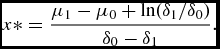
that is to say that when δ1 > δ0, the probability of migrating will be strictly increasing in x while when δ1 < δ0, the probability will first be increasing in x and then may become decreasing for x large enough. Define x* as P′(x*) = 0, which implies that
 \begin{equation*}
x*=\frac{\mu _1-\mu _0+\ln (\delta _1/\delta _0)}{\delta _0-\delta _1}.
\end{equation*}
It can easily be shown that  $\frac{\partial P(x)}{\partial \mu _0}=w_0 \frac{\partial P(x)}{\partial M}<0$. We can also show that there is a maximum skill level (xmax) above which nobody will ever migrate since in that case, w 1(xmax) − w 0(xmax) − M = a.
Once the economic incentives restriction is satisfied, the worker must be able to finance the migration cost in order to migrate. Let S(w 0(μ0, δ0, x)) be the resources available to a migrant with skills x. Thus, he can only migrate if:
 \begin{equation*}
S(w_0)>M.
\end{equation*}
We will denote the minimum level of skills that allow an individual to pay for the migration cost as xlc > 0. The difference between this liquidity constraint restriction and the one presented in Orrenius and Zavodny (Reference Orrenius and Zavodny2005) is that this specification considers the fact that the financing depends on current wages and so an increase in the outputFootnote 6 in the origin country helps the potential migrant to afford the migration cost. Specifically, 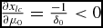 $\frac{\partial x_{lc}}{\partial \mu _0}=\frac{-1}{\delta _0}<0$ and
 $\frac{\partial x_{lc}}{\partial M}=\frac{1}{S^{\prime }(w_0) w_0\delta _0}>0$.
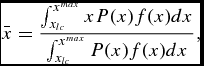
Overall, assuming that in a given country the distribution of skills over [0, +∞) is given by f(x), the average skills of migrants will be given by
 \begin{equation*}
\bar{x}=\frac{\int ^{x^{max}}_{x_{lc}} xP(x)f(x)dx}{\int ^{x^{max}}_{x_{lc}} P(x)f(x)dx},
\end{equation*}
where the denominator represents n, the number of migrants.
We can observe that once the two restrictions are taken into account this model suggests that if the skill price is bigger in the origin country migrants come from the middle part of the distribution, supporting the intermediate selection evidence found in (Chiquiar and Hanson, Reference Chiquiar and Hanson2005; Orrenius and Zavodny, Reference Orrenius and Zavodny2005; Mishra, Reference Mishra2007; Mckenzie and Rapoport, Reference McKenzie and Rapoport2007).
2.2 Comparative Statics
The model provides us with empirical predictions related to three variables that we can empirically observe: output in the origin country (GDP), migration costs and inequality.
Proposition 1.An increase in μ0reduces the average skill level of migrants unambiguously if ∂2P/∂μ0∂x ⩽ 0 and if the average migrant has worse amount of skill than the population of the sending country with skills such that they could potentially migrate. The impact on the number of migrants is uncertain.
Proof.
 \begin{eqnarray*}
\frac{\partial \bar{x}}{\partial \mu _0}&=&\frac{1}{n}\left(\left(\frac{x_{lc}P(x_{lc})f(x_{lc})}{\delta _0}+\int ^{x^{max}}_{x_{lc}} x\frac{\partial P}{\partial \mu _0}f(x)dx\right)\right.\\
&&\quad\left. -\,\bar{x}\left(\frac{P(x_{lc}) f(x_{lc})}{\delta _0}+\int ^{x^{max}}_{x_{lc}} \frac{\partial P}{\partial \mu _0} f(x)dx\right)\right)\\
&=&\frac{1}{n}\left(\frac{P(x_{lc})f(x_{lc})}{\delta _0}(x_{lc}-\bar{x}) +\int ^{\bar{x}}_{x_{lc}} (x-\bar{x})\frac{\partial P}{\partial \mu _0}f(x)dx \right.\\
&&\quad\left. +\,\int ^{x^{max}}_{\bar{x}} (x-\bar{x})\frac{\partial P}{\partial \mu _0}f(x)dx\right)\\
&<&\frac{1}{n}\left(\frac{P(x_{lc})f(x_{lc})}{\delta _0}(x_{lc}-\bar{x}) +\frac{\partial P(\bar{x})}{\partial \mu _0}\int ^{x^{max}}_{x_{lc}} (x-\bar{x})f(x)dx\right)\\
&<&\frac{1}{n}\left(\frac{P(x_{lc})f(x_{lc})}{\delta _0}(x_{lc}-\bar{x}) +(1-F(x_{lc}))\frac{\partial P(\bar{x})}{\partial \mu _0}\left(E(x|x>x_{lc})-\bar{x}\right)\right).
\end{eqnarray*}
The first term of the sum, which reflects the impact of μ0 in the liquidity constraint restriction, is clearly negative in all cases. Intuitively, this result reflects the fact that an increase in output in the sending country relaxes the liquidity constraint restriction and thus allows more unskilled workers to finance the migration cost.
The second term of the sum is an upper bound of the impact of an increase of μ0 that operates through the economic disincentive to migrate for all potential migrants. This term will be negative when the average migrant has worse amount of skill than the population of the sending country that could satisfy the liquidity constraint.
The conditions we have imposed imply that xlc is sufficiently large so that P(x)f(x) is decreasing faster in x than f(x), which ensures that we observe negative selection. The additional condition we have imposed, namely that ∂2P/∂μ0∂x < 0, will be satisfied if g′(ε) is decreasing when x > x*. If the liquidity constraint is too low, and in particular when xlc < x*, the average skill level of migrants may or may not decrease when μ0 is increasing as our conditions are unlikely to hold in this case. The impact on the number of migrants is uncertain as can be seen from the derivative of the denominator of  $\bar{x}$. ■
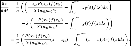
Proposition 2.An increase in M has an ambiguous effect on the average skill level of migrants but always decreases their number.
Proof.
 \begin{eqnarray*}
\frac{\partial \bar{x}}{\partial M}&=&\frac{1}{n}\left(\left(\frac{-x_{lc}P(x_{lc})f(x_{lc})}{S^{\prime }(w_0) w_0\delta _0}-\int ^{x^{max}}_{x_{lc}} xg(\varepsilon )f(x)dx\right)\right.\\
&&\quad\left. -\,\bar{x}\left(\frac{-P(x_{lc}) f(x_{lc})}{S^{\prime }(w_0) w_0\delta _0}-\int ^{x^{max}}_{x_{lc}} g(\varepsilon )f(x)dx\right)\right)\\
&=&\frac{1}{n}\left(\frac{P(x_{lc})f(x_{lc})}{S^{\prime }(w_0) w_0\delta _0}(\bar{x}-x_{lc})-\int ^{x^{max}}_{x_{lc}} (x-\bar{x})g(\varepsilon )f(x)dx\right).
\end{eqnarray*}
As before, the second term will be negative when ∂2P/∂M∂x < 0 and when  $E(x|x>x_{lc})>\bar{x}$, but the first term is now positive because an increase in M makes the liquidity constraint more binding. The overall sign of the equation is thus uncertain. However, the denominator of
 $\bar{x}$ is clearly decreasing in M.
 $\Box$■
Finally, a change in inequality will affect differently the average skill of migrants and their number, depending on where xlc is located in the distribution. Define
 \begin{equation*}
\sigma =\int ^{\infty }_{0} x^2 f(x)dx - \left(\int ^{\infty }_{0} x f(x)dx\right)^2,
\end{equation*}
that is to say, the variance in the distribution of x in the population of the country of origin. Then, a change in variance will impact the average skills of workers in the following way:
 \begin{equation*}
\frac{\partial \bar{x}}{\partial \sigma }=\frac{1}{n}\int ^{x^{max}}_{x_{lc}} (x-\bar{x})P(x)\frac{\partial f}{\partial \sigma }dx.
\end{equation*}
In the case where the liquidity constraint allows only individuals of sufficiently high skill to migrate, an increase in inequality (understood as a fattening of the tails) would increase the number of migrants and increase their average quality. This is because if xlc is sufficiently high, we would expect that ∂f/∂σ > 0 for all x > xlc. If the liquidity constraint is not so high that the fattening of the lower tail will include regions of the distribution from which migrants will be drawn, the number of migrants may fall and their average quality could increase or decrease.
If we were to extend this model to one where the decision to migrate includes, in addition, the problem of which location to select, our main conclusions would likely remain unchanged. An increase in the unskilled wage in the home country is likely to induce a decrease in the average skills of migrants to both destinations and unless this is coupled by a change in the returns to skill in the two destination country, it should also increase the average skills of migrants that go to each destination. A fall in the costs of migration to both of these countries would also generate an increase in the number of migrants to both countries and still an ambiguous effect on the average quality of migrants. We thus do not feel that the simplification we made regarding the number of destinations is likely to change our comparative statics in a significant way, nor invalidate our empirical results.
How does this model inform the empirical analysis that follows? The comparative statics we have derived suggest that the impact of each parameter will depend on a number of home country-specific characteristics as captured by the distribution of skills, the average wage, etc. We will approximate those using fixed effects for each country, a set of country-specific controls and, in some cases, country-specific linear trends or the interaction of initial conditions with year fixed effects. The equations we obtain also suggest that it is important to control for what is happening in the destination country. We will use time fixed effects to approximate this, as well as any other shocks to alternative destinations that would impact the sending countries in our sample. Finally, the theoretical exercise does not suggest a particular functional form for the relationship between average immigrant skills and our variables of interest. There is no sense that the relationship is clearly linear or even increasing or decreasing. For this reason, we will evaluate a number of specifications in the empirical section.
Some further explanations need to be given in translating our model to the data. We will use proxies for our variables that suffer from some measurement error. To proxy for μ0, we will use log GDP per capita. This is not the log of the wage of a person with a skill of zero but is the only measure we dispose of. However, the evolution of the GDP in capita in a country would differ from the evolution of μ0 only because of two alternative reasons. The first is that the distribution of x is changing. If that was the case, however, we anticipate that this would lead our GDP measure to be positively correlated with the average skills of migrants as the improved skills of the domestic population would translate into better migrants, ceteris paribus. The only situation in which a rightward shift in the distribution of x could lower the average skills of immigrants is if this increase is such that it increases the mass of workers more importantly in the region where the propensity to migrate is high than where it is low. In our model, since P′(x) < 0, this implies that the shock would increase mostly the number of individuals particularly close to the liquidity constraint. This is likely to happen only if there is substantial positive selection, something we will test further on. The second reason why GDP per capita could increase without a change in μ0 is because the returns to skill in the sending country could improve but actually, the comparative statics for δ0 are relatively similar to those with respect to μ0, making this also a valid interpretation. To proxy for costs, we will use a measure related to the costs of transportation from the country of origin to the United States. Clearly, moving costs also include additional elements but we anticipate that these would be positively correlated with our proxy measure.
3 EMPIRICAL MODEL
In order to evaluate the empirical predictions, we use the regression equation:
 \begin{equation}
\ln x_{ct}= \beta _0+ \beta _1 \ln u_{0ct} +\beta _2 \ln M_{ct} +\beta _3 C_{ct}+ \phi _c+\theta _t+\epsilon _{ct}.
\end{equation}
Where c represents the country of origin, t a given year and x represents the average skill level of immigrants. u 0ct denotes the output level in the origin country and Mct the migration cost. C is a set of control variables representing other relevant factors as political stability, education, population, trade, and government revenue and expenditure, which will be included in some specifications. ϕc and θt are country and time fixed effects and εct is the error term. This functional form is commonly used in panel data literature. For example, Mayda (Reference Mayda2010) performs the largest panel data analysis on determinants of migration using the same specification. The logarithmic assumption on the explanatory variables is made to control for changes in percentage as opposed to levels in GDP so the scale of the country is taken into account and does not distort the analysis. The logarithmic assumption on the dependent variable allows us to estimate elasticities and semi-elasticities and thus compare the coefficients associated to the different skill level measures that we will use. The country and year fixed effects, which represents the main gain from using a panel data, control for idiosyncratic and unobservable characteristics of each country and year. The country fixed effects capture the time-invariant cross-country variation that affect the skill level of immigrants as the culture of the country or the persistent component of inequality. On the other hand, the year fixed effects control for every shock to skill level of immigrants in a particular year that is common to all the countries. Very importantly, this includes the economic conditions in the US, that are very relevant for the economic incentives component of the migration decision as our model suggests.
In order to test the cross-country effect of persistent inequality, we will use the country fixed-effects estimated in the equation (5):
 \begin{equation}
\hat{\phi _c}=\beta _4 + \beta _5 \sigma ^2_{c}+e_c.
\end{equation}
This methodology of identification in two stages is based on the fact that country fixed effects capture the cross-country differences in skill level that are not explained by the independent variables on the first stageFootnote 7. This empirical setting resembles the more informal analysis performed by Borjas (Reference Borjas1987) to test his empirical prediction about the effect of inequality over immigrants’ skill.
In an ideal empirical model, we would like to test the effect of inequality on immigrants’ skills using not only cross-country variation but also time variation, allowing us to use the fixed effects in order to control for non-observables related to the specific periods or origin country. That strategy would require “flow” inequality data as skill prices or alternatively an inequality by cohort measure taken out of an age-cohort-period decomposition, because the “stock” inequality as measured by Gini is very persistent over time and does not capture much underlying variation of inequality over time. Because there is no inequality data (either “flow” or “stock”) for such an old time span, and given that inequality is very persistent, we use modern cross-country inequality data to perform this empirical exercise and are thus cautious in the interpretation of the results.
4 DESCRIPTION OF THE DATA
Having described the empirical strategy, we now turn to the construction of the variables of interest. The empirical strategy presented above requires annual GDP and political stability variation at the country level. This reduce our sample to 39 countries for which such data is available. Even though many countries are left out of the sample, the 39 countries included represent approximately 92% of the total immigrant flow in the period, as they included all the large European countries and the largest American and Asian countries (see Appendix A.1 for a list of the countries included).
4.1 Amount and Skill Level of Immigrants (x)
Quantity and skill level of immigrants for each country were taken from the Report of the Commissioner of Immigration (henceforth, RCI), which corresponds to administrative data presented as summary tables based on questionnaires that every immigrant had to answer at departure from the origin country or at their arrival to the USFootnote 8. The RCI was published annually from 1899 to 1932 (except for 1931) and provides data on the ethnic origin and on self-reported occupation that each immigrant performed before migrating. This data is useful to evaluate our empirical question because, in contrast with other macro data used in the literature which used occupations or wages of the immigrants had in the US, the RCI allows us to measure the quality of the occupations immigrants had before they arrived to the US. This is a better measure of actual skills if, as suggested by the literature (Borjas, Reference Borjas1987, and Lafortune and Tessada, Reference Lafortune and Tessada2014), the immigrants take some time to assimilate to the US labor market and also the US labor market takes some time to identify or use the skills of immigrants. Furthermore, the time span covered by the data gives us the rare opportunity to characterize the self-selection process in an open gate environment, because before the restrictions on immigration imposed in the 1920s, immigrants from most countries had no major obstacles entering the US, so the only factors determining the characteristics of immigrants were whether they had incentives to migrate and the means to afford it. This feature of the period also validates the self-reported information as there were no incentives to lie about past occupation.
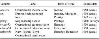
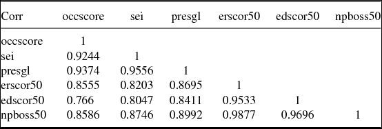
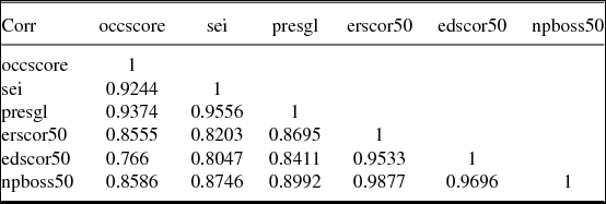
Despite of the advantages of the RCI data, there are challenges related to the adaptation of the data to our empirical design. First of all, occupational data must be matched with some skill level indicator. For this purpose, we use the occupational standing variables from the United States Census as presented in the Public Use Micro Sample (henceforth, IPUMS). These variables are quality measures associated to the occupational classification of the 1950 United States Census. The basis for each quality score and the source data are presented in Table 1. In Table 2, we can see the correlation between these variables for individuals included in the 1900, 1910, 1920 and 1930 US census. The first three variables, associated more strongly to income and prestige, and the last three variables, associated to education and earnings, have large correlation between them and smaller ones with the other three variables. This distinction will be useful in the empirical results analysis.
Occupational standing variables description

Correlation between occupational standing variables
Before applying these quality measures to our occupational information, we must match the occupations from the RCI to the occupation classification of 1950 census. To accomplish that we used the matching constructed by Lafortune and Tessada (Reference Lafortune and Tessada2014)Footnote 9. Another challenge is presented by the fact that the information taken from RCI data is aggregated at ethnic group level and the GDP, cost and control variables are measured at a country level. The approach we took is to transform ethnic group level occupational data to country level data. In order to do that, we again used the matching between countries and ethnic group done by Lafortune and Tessada (Reference Lafortune and Tessada2014). Provided that there is more than one country matched to each ethnic group, we divided the flow of the ethnic groups between its corresponding countries calculating, for each occupation and year, the share of the total inflow of an ethnic group that corresponds to a particular country according to the IPUMS data. That is, we measured in IPUMS the amount of immigrants from each country and occupation that arrived in a particular year, aggregated them into ethnic groups, and then calculated the shares of each country. Then, we used the shares for each year and occupation to divide the inflow of an ethnic group that appear on the RCI data on countries. This methodology is assuming that immigrants that stayed in the US, and thus appeared in the decennial census, are randomly selected from each country inside an ethnic group, so the shares that appear in the IPUMS are a good approximation of the actual shares at the time of entrance to the country. As an alternative methodology, we used the same shares calculated for each country-year-occupation to aggregate the independent variables at ethnic group level. The differences between these two methodologies are explained in the empirical results section.
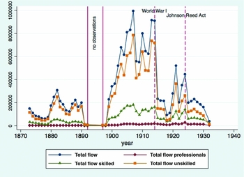
Besides the information on the occupation of the migrant, the RCI categorizes each occupation as professional, skilled or unskilled.Footnote 10Figure 1 presents the total flow divided by skill level of all the immigrants for each year. This aggregated data give us a broad understanding of the immigration process that is the subject of this study. The first important feature of this data that is worth mentioning is the big fall in total flow that happened between 1890 and 1898. Even though we have missing data between 1893 and 1897, the low levels of immigration flows in 1891, 1892 and 1898 confirm the historical finding that the US bad economic conditions of the 1890sFootnote 11 made migration to the US undesirable (O’Rourke and Williamson, Reference O’Rourke and Williamson2001). After that slum, from 1899 to 1914 we observe a big wave of immigration that is dramatically interrupted by World War I (henceforth, WWI). Another historical event that had evident impact on immigration is the Johnson–Reed Act of 1924, that imposed restrictive quotas on immigrants from all countries, specially from eastern Europe and Asia. These quotas had an effect on the flow of immigrants of the three skill levels, not only on unskilled immigrants.
Total, professional, skilled and unskilled flow for each year.

4.2 Stock of Migrants by Ethnic Origin
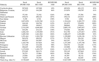
The RCI data provide not only data on immigrants but also on out migration of returning migrants for each ethnicity and year from 1909 onFootnote 12. In combination with the US Census micro samples (IPUMS), we can use this inflow and outflow data to construct the stock of migrants from a specific ethnic origin living in the US at the beginning of each year. In order to do that we take from IPUMS the stock in 1910, 1920 and 1930 for each ethnicity and add the net inflow (inflow minus outflow) of each year to calculate next year stock (US Census were taken approximately at the beginning of each year). As we can see in Table 3, this procedure give us an estimation of the decennial net inflow that is not necessarily precise according to the next decade census, because it does not account for mortality and births on the destination country and may be affected by measurement error. To account for that estimation error of the net inflow, we take the difference between the RCI predicted stock at the beginning of each decade and the stock presented in the census and we assign one tenth of that difference to the net inflow of each year of the preceding decade. With that procedure, the predicted stock is now the same that the stock presented in the census and there is no jump in the stock estimation at the end of each decade.
Comparison of stock measures for ethnicities using IPUMS and RCI data

With this ethnic stock measure, we assign to each country the stock of the ethnic group corresponding to the country, so two countries can be associated with the same ethnicity stock. Provided the limitations of the return migration data and the missing observation of 1931, this variable is constructed only from 1910 to 1930.
4.3 Migration Cost (M)
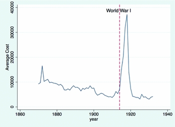
This variable is constructed using the distance to the US multiplied by the freight rate (cost of delivering a cargo from one point to another) of transporting commodities to Europe from the closest route for each country and period taken from Mohammed and Williamson (Reference Mohammed and Williamson2004)Footnote 13. Figure 2 shows the average migration cost for each period. Coherently with the fall on immigration flow during the WWI observed in Figure 1, freight rates during that period had a huge spike reaching a peak in 1917, followed by a normalization. Omitting this shock, the graph suggests a strong decline in immigration costs until WWI.
Average migration costs for each year.

4.4 GDP Per Capita (μo)
We took Purchasing Power Parity GDP per capita data available from Maddison’s “Historical Statistics of the World Economy” and from Barro and Ursúa (Reference Barro and Ursúa2010) Macroeconomic data. In order to match both databases, we took both samples to the same base year (2006 is 100) and maintain the integrity of the data for each country so there is no mixed data for one country. One concern about using GDP per capita is that workers react to wage differentials between the origin and destination countries and GDP may not necessarily be strongly correlated with wages in the presence of wars or other economic circumstances. In order to address this concern, we use data on European wagesFootnote 14 for our period of study from Williamson (Reference Williamson1995) and calculate the elasticity of wages to changes in GDP. The estimated elasticity of wages to GDP is 0.44 with a 0.066 standard deviation. This result confirms that GDP and wages are positively and strongly correlated.
4.5 Inequality (σ2)
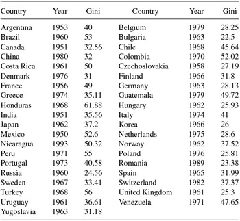
This variable is estimated using the inequality data from Deininger and Squire (Reference Deininger and Squire1996) database. This dataset encompasses all the inequality data that is available from different sources. As it was stated in the presentation of the empirical model, there is no inequality data for the time span of our study so we proxy the Gini of each country using the first available Gini data.Footnote 15 This methodology relies on the persistence of the stock inequality measures to assume that Gini data from mid XXth century is a good approximation of Gini on early XXth century. This measurement error should attenuate the coefficients estimates.
4.6 Controls (C)
We control for political stability in every regression using a participation in international wars dummy from the Correlates of Wars Project and a level of democracy indicator (polity2) taken from the polity IV database. This democracy level indicator range from -10 (hereditary monarchy) to +10 (consolidated democracy). In some specifications, we also control for education (primary education enrollment and secondary education enrollment), population, trade per capita, and government revenue and expenditure per capita. These variables were taken from the CNTS (Cross-National Time-Series) data.
5 EMPIRICAL RESULTS
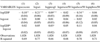
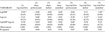
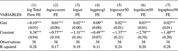
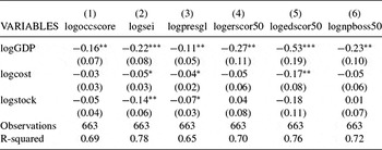
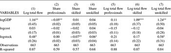
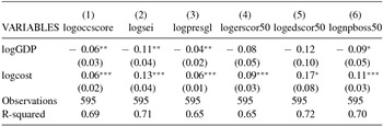
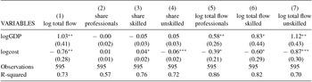
Our theoretical model makes predictions regarding the impact of output, mobility costs and inequality over average skill level and quantity of immigrants. In Table 4, we present the results of estimating our empirical model with the six described measures of average skill level as the dependent variable and Table 5 shows the results for total quantity and professional, skilled and unskilled immigrants quantities. Both tables describe the impact of GDP and migration cost from different angles and in particular Table 5 allows us to understand the underlying changes in quantities that drive the changes in average skill level. We include the interaction between GDP and cost to analyze if both factors are interrelated. For the interaction terms the logarithm of GDP and the logarithm of cost are expressed as difference from the mean of those logarithms for the whole sample, in order to maintain the coefficient of the main effect unalteredFootnote 16 The second stage regressions that evaluate the impact of inequality are presented in Tables 6 and A.2.
Skill level regressions

*** p < 0.01, ** p < 0.05, * p < 0.1
Notes: Clustered standard errors at a country level. Controls for democracy level, international wars and year and country fixed effects are included. The dependent variables are the average score in occupational standing variables (see Table 1). An observation correspond to a country in a year.
Quantities and shares regressions

*** p < 0.01, ** p < 0.05, * p < 0.1
Notes: Clustered standard errors at a country level. Controls for democracy level, international wars and year and country fixed effects are included. The dependent variables are quantities and shares of immigrants for each skill category. An observation correspond to a country in a year.
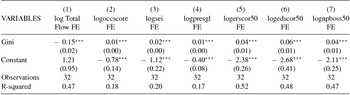
Fixed effects regressions on Gini

*** p < 0.01, ** p < 0.05, * p < 0.1
Notes: Robust standard errors in parenthesis. The dependent variables are the country fixed effects estimated in the regressions presented in Tables 4 and 5 . The regressions are weighted by the inverse of the standard deviation estimated for each fixed effect to account for the fact that the dependent variable is an estimation (this increase the standard deviation but does not affect the coefficients estimation). An observation correspond to a country.
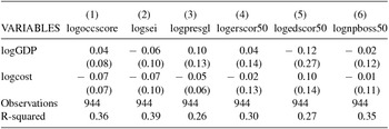
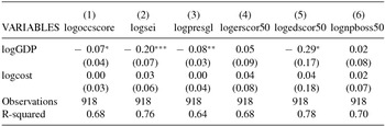
The results in Table 4 show that for the three first occupational standing variables, associated with income and prestige, and for the educational score, an increase in GDP per capita decreases significantly the average skill level of migrants. For the other two variables, associated with earnings and education, the result is the same sign but it is not statistically significant. This is consistent with the theoretical finding that an increase in origin’s country output decreases the economic incentives for high-skilled individuals to migrate and relax the liquidity constraint, resulting in more low-skill individuals migrating if the liquidity constraint is binding. The magnitude of the estimated income elasticities ranges between a 0.9% to a 0.34% decrease in the occupational standing scores as a response to a 1% increase in GDP per capita. Qualitatively, this empirical finding is coherent with micro data evidence from Orrenius and Zavodny (Reference Orrenius and Zavodny2005) who find the same relation between output and skill level using variation between regions in Mexico. In contrast, Borjas (Reference Borjas1987) using a cross-country analysis find that countries with bigger GDP per capita have better wages in the US. The differences between these two results may be explained by the fact that wages in the US can correlate better with skill for richer countries with similar production structuresFootnote 17 or by unobservables that a cross-country design is not able to capture.
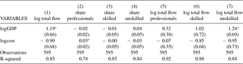
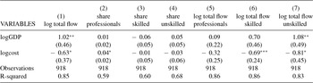
In order to identify which of the mechanisms presented in the model are actually explaining the results of Table 4, Table 5 shows the correlation of our explanatory variables with the quantities and shares of professionals, skilled and unskilled individuals that immigrate from each country. An increase in GDP raises the total amount of immigrants of all skill levels, implying that the liquidity constraint restriction is important and is binding not only for unskilled workers but also for some skilled and professional workers. Nevertheless, the increase in the inflow is bigger and statistically significant for unskilled workers, suggesting that the liquidity constraint restriction is more important for them. An implication of this result is that it confirms that, as considered in our model, an increase in GDP in the origin country helps financing the mobility costs, because all other mechanisms by which GDP has an impact suggests that GDP decreases the quantity of migrants. Thus, while supporting our modeling strategy this result cannot be rationalized with neither Borjas (Reference Borjas1987) or Orrenius and Zavodny (Reference Orrenius and Zavodny2005) models.
A potential issue with the interpretation of these results is the possibility that changes in GDP reflect shifts in the skill distribution instead of changes in base wages or the skill premium. As stated in the model section, an increase in the average skill level of the population implies a larger average skill level of the migrants, unless there is a substantial positive selection. In order to evaluate if the negative effect of GDP over the average skill level is attenuated or reversed in countries where there is a higher share of skilled migrants, we include in our main regressions an interaction of GDP with a dummy for countries who send a large share of high-skilled workersFootnote 18. The results, available upon request, show that the interaction is not significant, which indicates that shifts in the underlying distribution are not driving our results.
The coefficients for migration cost in Table 4 show that an increase in migration costs does not have a significant impact on average skill level. In the second row of Table 5 we can see that, as theoretically expected, migration costs affect negatively the quantity of immigrants from all skill levels, but the shares of each skill level in the total flow are not altered and thus there is no aggregate effect on average skill level. This result may explain why Borjas (Reference Borjas1987) finds that distance to the US, which is the time invariant component of our mobility cost, has no significant effect over the immigrants wages in the US. In contrast, Orrenius and Zavodny (Reference Orrenius and Zavodny2005) find that migration costs increase the average skill level. The difference in both results does not necessarily implies that one of the results is empirically wrong as in theory a negative, neutral, or a positive effect can be found depending on the relative relevance of the liquidity constraint restriction and the economic incentives restriction in the time period and countries of analysis. However, our results are consistent with our theoretical model.
The results for the interaction in Tables 4 and 5 show that in countries with largest migration costs an increase in GDP induce an even larger positive effect on quantity of migrants from all skill level, but as expected as the migration costs get larger an increase in GDP has a stronger effect on skilled people, because they are more affected by liquidity constraints in these countries with larger migration costs.
5.1 Second Stage: Gini Regressions
Table 6 shows the regression of the country fixed effects estimated by the skill level and quantities regressions for 1899–1932 (Tables 4 and 5) against a proxy of the Gini of each country.Footnote 19 The results indicate that more unequal countries provide immigrants with a higher skill level. In terms of our empirical predictions, this would be the case if the reduction in low-skilled migrants is more important in terms of the average skill level than the reduction on high-skilled migrants. Also, as presented in column (1), the Gini appears to have a strong negative effect over the total flow of migrants which is what the model predicted if the liquidity constraint is binding and the economic incentives to migrate for high-skilled individuals decrease.
This kind of simple exercise is analogous to the one that Borjas (Reference Borjas1987) uses to confirm his hypothesis that bigger inequality implies less skilled immigrants. Nevertheless, we should be careful with interpreting these results as conclusive evidence, because we are only using cross-country data on income inequality (as opposed to skill inequality) that does not allow us to control for country unobservables as we have done in the previous regressions. In order to address this concern, in Appendix A we incorporate controls for plausible covariates of skill level in the first stage (skill level regressions) so the country fixed effects variation does not reflect variation in these variables. Specifically, we add controls for education (primary education enrollment lagged by 9 years and secondary education enrollment lagged by 5 years), population, trade per capita, and government revenue and expenditure per capita. The results are unchanged.
5.2 The Role of Stock of Migrants in the US
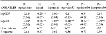
As emphasized by Carrington et al. (Reference Carrington, Detragiache and Vishwanath1996), one of the most important dynamic aspects of the migration process is the fact that migrants generate networks in the destination countries that reduce the migration costs for the following waves of immigrants. This fact has also been empirically described by Munshi (Reference Munshi2003) and Lafortune and Tessada (Reference Lafortune and Tessada2014). Our panel data design and the availability of a measure of the stock of migrants from a specific ethnic origin give us a remarkable opportunity to test these network channel at an aggregate country level. Theoretically, if networks reduce the mobility cost then an increase in the stock of migrants from an ethnic origin should increase the number of migrants. Despite the fact that the stock variable is only available from 1910 to 1930, this prediction is confirmed by Tables 7 and 8. In particular, we observe that an increase in stock increases the total quantity of migrants from all skill levels but this positive effect is bigger and statistically significant for unskilled workers, so the average skill level decreases. According to Beine et al. (Reference Beine, Docquier and Ozden2011), the same results apply to modern migration to the OECD countries, suggesting that the network channel has been an important feature of the migration phenomena throughout history and in particular bigger networks implies more but less educated immigrants.
Skill level regressions

*** p < 0.01, ** p < 0.05, * p < 0.1
Notes: Clustered standard errors at a country level. Controls for democracy level, international wars and year and country fixed effects are included. The dependent variables are the average score in occupational standing variables (see Table 1). An observation correspond to a country in a year.
Quantities and shares regressions: 1910–1930

*** p < 0.01, ** p < 0.05, * p < 0.1
Notes: Clustered standard errors at a country level. Controls for democracy level, international wars and year and country fixed effects are included. The dependent variables are quantities and shares of immigrants for each skill category. An observation correspond to a country in a year.
5.3 Restrictions Impact Assessment
The first important restriction imposed in the period under study is the Chinese Exclusion Act of 1882 which prohibited all immigration of Chinese low-skilled workers (O’Rourke and Williamson, Reference O’Rourke and Williamson2001). The prohibition was a reaction to the strength in competition of the supply of low-skilled workers in California. The next important restriction imposed was the 1917 Immigration Act.Footnote 20 This act excluded from entry immigrants from all the countries inside the “Asian Barred Zone” that included all the major countries of Asia with the exception of Japan and the Philippines. Later, in 1921, a new Immigration Act aimed at reducing the inflow from eastern and southern Europe by the imposition of quotas that were calculated as a 3% of the foreign-born population from each country that appeared in the 1910 census. These quotas were more restrictive for the late waves of immigration that came from southern and eastern Europe and that in 1910 had not yet settled massively in the US. Finally, in 1924 the Johnson–Reed Act of Immigration recalculated the quotas as a 2% of the population with foreign originFootnote 21 from each country that appeared in the 1890 census and prohibited the entry of Japanese low-skilled workers. This final Immigration Act, that was not revised until 1952, restricted immigration from all the countries in Europe. In contrast, none of these immigration acts were imposed on Latin American countries.
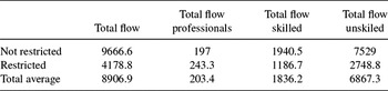
Using these historical data, we construct a dummy that indicates for each country the years after which binding restrictions were imposed on immigration. Thus, China start being restricted after 1882, Asian countries excluding Japan start being restricted after 1917, eastern and southern European countries start being restricted after 1921 and finally the rest of Europe and Japan start being restricted after 1924. In Table 9, the effects of the restrictions can be clearly seen. As expected, restrictions decreased strongly the total flow of unskilled and skilled while the flow of professionals increased.
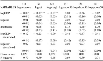
Descriptive statistics for restricted and unrestricted observations

In Table 10, we use this dummy to estimate the impact of our determinants in an environment free of restriction and to assess the effect of regulation over the selection process and over the effect of the determinants. In order to do that, interactions with the logarithm of GDP and the logarithm of mobility cost are included. The first two rows confirm that our main results represent the selection process that took place when no restriction were imposed over immigration. Also, the point estimates of the restriction dummy coefficients suggest that the restriction increases the average skill level but only with statistical significance for the education measure, which may reflect the fact that the restrictions focused on literacy and other measures of formal education. Finally, restrictions do not reverse the negative effect of GDP over average skill level, suggesting that the liquidity constraint restriction is, if anything, more relevant in a restricted environment for immigrants.
Skill level regressions with dummy for restricted countries

*** p < 0.01, ** p < 0.05, * p < 0.1
Notes: Clustered standard errors at a country level. Controls for democracy level, international wars and year and country fixed effects are included. The dependent variables are the average score in occupational standing variables (see Table 1). An observation correspond to a country in a year.
5.4 Regressions Using IPUMS Data
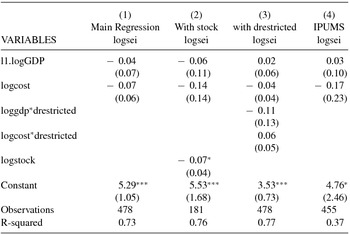
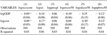
There are two main differences between using IPUMS occupational data and using, as in the previous regressions, the RCI administrative data. First, immigrants that appear in the decennial US census are the ones that stayed in the country while RCI data capture all the immigrants that arrived to the US. Hence, IPUMS data reflects in part the return migration selection process. Second, occupational data from IPUMS describe the occupations that immigrants had in the US, while the RCI data contains information on the occupations immigrants performed in their origin country. In Table 11, we observe that when IPUMS data is used to construct the dependent variables our explanatory variables do not have an effect on the average occupational scores of immigrants in the United States. This important difference with our previous findings cannot be entirely attributed to return migration, because the return migration decision, even if determined by similar variables, is made at a different timing than the original migration decision. Thus, it is unlikely that the return migration selection reverses the original selection process in such a way that we no longer can identify the effects of the determinants of the migration decision. Furthermore, the empirical literature about return migration (Coulon and Piracha, Reference Coulon and Piracha2005; Ambrosini and Peri, Reference Ambrosini and Peri2012; Aguilar Esteva, 2013) found mixed evidence on whether the return migrants are the less or more skilled, but never makes any links between the determinants of the original migration decision and this issue.
Skill level regressions using IPUMS data

*** p < 0.01, ** p < 0.05, * p < 0.1
Notes: Clustered standard errors at a country level. Controls for democracy level, international wars and year and country fixed effects are included. The dependent variables are the average score in occupational standing variables (see Table 1). An observation correspond to a country in a year.
Another hypothesis is that the determinants of the migration decision have no effect on the average occupational scores because the occupations that immigrants had on the US were not reflecting their skills. This would be the case if the US labor market is not able to recognize or use the immigrants skill once they arrived but only after an assimilation process. This hypothesis was proposed and empirically confirmed by Borjas (Reference Borjas1987) and more recently by Lafortune and Tessada (Reference Lafortune and Tessada2014). Thus, the results presented in Table 11 can be interpreted as suggestive evidence of the existence of an assimilation process in which the US labor market is not able to take advantage of the immigrant skills. Moreover, these results demonstrate that using occupations of migrants in the US as a measure of skill level may lead to wrong conclusions.
5.5 Robustness Checks
In order to address potential endogeneity problems with the estimation of a causal impact of GDP over skill level (our measure of mobility cost is exogenous), in Appendix we add controls for variables that can affect both the GDP of a country and its average skill level. Specifically, we add controls for education (primary enrollment lagged by 9 year and secondary enrollment lagged by 5 yearsFootnote 22), population, international trade per capita and government revenue and expenditure per capita. Also, we use one lag of GDP instead of GDP to avoid the possibility of reverse causality. In Table B.1, the results for the main specifications the we have analyzed are presented focusing on one skill level measure for presentation purposes.Footnote 23 Even though there is an important loss of observations that increases the standard deviation of the coefficients, the point estimates are confirmed, suggesting that our results are not driven by omission of these variables. We do lose statistical significance, however. The addition of lags and controls for possible confounding variables does not dismiss all sources of potential endogeneity. Nevertheless, the fact that our main results qualitatively survive to these exercises is indicative that the results are explained by the proposed mechanism and not by other plausible interpretations.
Another robustness check consists in repeating the analysis at an ethnicity level instead of country level. Instead of decomposing the dependent variable as was done before, we aggregated the independent variables from a country level to an ethnicity level using the same shares. There are two main differences between these methodologies that made the country level data preferable. First, at a country level data we have more observations and if GDP or political stability data is missing, we only miss that individual country observation. At an ethnicity level data, if one of the countries corresponding to that ethnicity have missing GDP data, we lose the whole ethnicity observation for that year, because we cannot compare across time between weighted sums of different countries. Second, considering that the shares are constructed imperfectly using information only about the immigrants who stayed (IPUMS data), if we have measurement error in the dependent variables, as we do at a country level, we only lose statistical significance as the dependent variable has more error but we do not introduce bias in the coefficient estimation. If we use the data at an ethnicity level, we have bigger measurement error in the dependent variable and that leads to attenuation bias in the estimation of the coefficient, so the point estimation should be closer to 0.
The skill level regressions at ethnic group level are presented in Table C.1 and Table C.2 on the Appendix C. The results for GDP are still negative and significant for most specifications but the point estimates are smaller, which is to be expected because of the aforementioned attenuation bias. The results for migration costs differ and we have that at an ethnicity level the regressions show that the average skill level increases as a response of bigger migration costs because the quantity of unskilled migrants decreases the most. As we have argued, the effect of mobility cost on average skill level is theoretically ambiguous and it depends on the relative importance of both restrictions in the specific country and period. Since the regressions at an ethnic group level do not aggregate the information of all the observations that we have at a country level, it is possible that the selection of the observations that can be aggregated at an ethnic group level is the reason why both results differ. To evaluate this possibility, in Table C.3 we show the regressions at a country level that only includes the observations that can be aggregated at an ethnic group level. As we can see, the results for migration costs at a country level are now consistent with the results at an ethnic group level, supporting our reasoning. These results again emphasizes the importance of liquidity constraints as a larger migration cost would make it more difficult for low-skill migrants to pay for their move, increasing the average skill level of migrants.
An empirical exercise that is necessary to validate our empirical strategy is to consider the fact emphasized by Bertoli and Fernández-Huertas Moraga (Reference Bertoli and Moraga2013) that changes in relevant variables of other possible destinations must be considered when analyzing the inflow of immigrants to one particular country, a phenomenon named by Bertoli and Fernández-Huertas Moraga (Reference Bertoli and Moraga2013) as “multilateral resistance to migration”. In particular, year fixed effects do not fully control for the impact of other destinations if such impact is heterogenous through sending countries. For example, changes in the UK will have a different impact on European countries compared to Asian countries. In order to address this possible heterogenous effect, we present in Table D.1 and Table D.2 the results of adding to our regressions year-continent fixed effects, that is, year fixed effects interacted with continent dummies.Footnote 24 These fixed effects control for factors that affect every country from a continent in a year, including changes in other possible destination countries. We run these regressions at an ethnic group level because as explained in the previous paragraph at an ethnic group level, we have a balanced panel which allows the composition of balanced year-continent groups. As we can observe, the results are qualitatively unaffected.
Finally, we exclude the WWI period from our data. This is important because for those years where we have a combination of extremely high mobility costs as evidenced by Figure 2, low GDP and political instability for many countries. If we limit our estimations and remove the WWI years, we obtain that our results are qualitatively the same as before.Footnote 25
6 CONCLUSIONS
One of the relevant factors that are key to understand the practical implications of migration and restrictions on migration is whether immigrants are high-skilled or low-skilled and what determines differences in occupational quality between immigrants from diverse nationalities. In this context, this paper contributes to the literature by identifying the determinants of the skill level of immigrants and their effect using a panel with data on occupations immigrants had before migrating that covers the mass migration period at the beginning of the twentieth century.
The empirical exercises support the theoretical finding that an increase in output has a negative effect over average skill level and suggests that the main channel by which changes in output affected the average skill level of migrants in that time period is through the easing or tightening of the liquidity constraints, a channel that was not present in previous models and should be considered in further theoretical research. In terms of policy, this result implies that by fomenting development in sending countries, a country may actually lower the quality of the immigrants it receives.
Another interesting finding is that the estimated negative impact of GDP on the average skill level of the occupations immigrants had before migrating does not translate in a decrease in the average skill level of the occupations of those immigrants who stayed in the US. This result calls for new research on the subject and suggests that the US labor market may not assimilate perfectly the skills of immigrants and thus using migrants’ occupation in the United States as measure of skills lead to misleading conclusions.
Finally, the availability of new panel data on immigration allows us to formulate empirical questions about the dynamics of the migration decision that were not covered in this paper but have an important role on the phenomena we are describing. How do expectations about future wage differentials are formed? In this paper, we found that output in the sending countries affect the average skill level mainly though the liquidity constraint restrictions and not through the economic incentives restriction as was previously thought. This is to be expected if we consider that the economic incentives to migrate depend mainly on future wage differential in specific occupations or skill sets that may not be strongly correlated with short term aggregate output fluctuations. In this context, in order to fully understand the role of economic incentives in the self-selection of migrants, we need to consider what kind information is taken into account when deciding whether to migrate or not. Potentially, private information dissemination through networks may create migration patterns that partly explained the timing and regional structure of the migration waves in the sending countries.
A GINI DATA AND ADDITIONAL SECOND STAGE REGRESSIONS
Gini data obtained from Deininger and Squire (Reference Deininger and Squire1996)

Second stage using fixed effects of regressions with controls

B REVERSE CAUSALITY AND POSSIBLE CONFOUNDING VARIABLES ASSESSMENT
Skill level regressions including controls for education, population, trade and government revenue and expenditure

C REGRESSIONS AT ETHNIC GROUP LEVEL
Skill level regressions at ethnic group level

Quantities and shares regressions at an ethnic group level

Skill level regressions at country level using observation available at an ethnic group level

D REGRESSIONS INCLUDING YEAR-CONTINENT FIXED EFFECTS
Skill level regressions including year-continent fixed effects at ethnic group level

Quantities and shares regressions including year-continent fixed effecs at an ethnic group level

E REGRESSIONS EXCLUDING WORLD WAR I
Skill level regressions excluding World War I

Quantities and shares regressions excluding World War I