

1 Introduction
Developed by Thaler and Benartzi (Reference Thaler and Benartzi2004) to help people save more for retirement, the Save More Tomorrow™ plan (or SMarT plan for short) has gained startling popularity with economists, the popular press, employees and politicians. Academic papers on 401(k) participation often cite the success of the SMarT plan as a major breakthrough in the application of behavioral economics to real world problems, and a large array of personal finance articles in the popular press reach the same conclusion. Workers at various firms in the US have eagerly enrolled in SMarT plans (Thaler and Benartzi, Reference Thaler and Benartzi2004), 65% of workers in the 2006 Retirement Confidence Survey say they would like to participate in a SMarT plan (Helman et al. Reference Helman, Copeland and VanDerhei2006), and the Pension Protection Act of 2006 encourages a SMarT default on 401(k) plans (Moore, Reference Moore2006; US Congress, 2006).
The reason for the remarkable popularity of the plan is that it is simple, yet quite clever. Participants commit today to save some fraction of future wage increases, which is appealing because it allows them to procrastinate saving more than what they are currently saving and because they are never required to consume less than their present level of consumption. In addition, inertia seems to keep people in the plan rather than expending the effort to opt out. The results in the pilot implementations were remarkable: saving rates among participants increased from 3.5 to 13.6% in just 40 months (Thaler and Benartzi, Reference Thaler and Benartzi2004). There is very little doubt that the SMarT plan is an effective device to help people save more for retirement.
In this paper, we examine an important question that has been on the minds of economists who study saving behavior (see, e.g., Choi et al. Reference Choi, Laibson, Madrian, Metrick, McCaffery and Slemrod2006): how close does the prescriptive SMarT plan come to approximating the normative life-cycle/permanent-income consumption rule? Our answer is that it can come quite close. We arrive at this conclusion by studying two types of consumers from the opposite ends of a spectrum. One type has perfect foresight, and so he optimally chooses to set period consumption equal to the annuity value of lifetime wealth according to the life-cycle/permanent-income model. This consumer, of course, does not need any help for saving adequately for retirement. The other type of consumer follows a suboptimal path, and therefore, he may benefit from participation in a SMarT plan in which he agrees to save a fixed fraction of future wage increases. In the absence of any SMarT plan participation, this second type of consumer follows a simple rule of thumb (by assumption) in which a low, constant fraction of wage income is saved in each period of the working years.Footnote 1 These consumers are unable to compute the optimal consumption plan, and so they follow a rule of thumb which in principle could lead to oversaving or undersaving, but our focus is on those with low saving rates. Such individuals accumulate low levels of wealth and experience a drop in consumption spending at the date of retirement since they are unable to maintain pre-retirement spending levels. Therefore, following a rule of thumb creates the possibility that a SMarT plan can help better smooth consumption over the life cycle, and we rigorously measure how well the SMarT saving program can help such consumers for approximating the optimal life-cycle/permanent-income consumption rule. Although the results sometimes vary widely across the various simulation experiments that we conduct, we generally find that participation in a SMarT plan is useful in helping a rule-of-thumb agent to overcome much of his otherwise inefficient use of lifetime resources.
Following the theoretical setup described in Section 2, our welfare analysis begins in Section 3 by computing the ‘wealth equivalent’, which we define as the amount of wealth that must be deducted from the lifetime resources of a life-cycle/permanent-income consumer in order to make his lifetime utility the same as the utility of an otherwise identical rule-of-thumb consumer. This is a measure of the implicit cost or inefficiency involved in following a rule-of-thumb consumption path rather than the optimal path. We then compute the ‘efficiency gain’ associated with SMarT plan participation, which we define as the fraction of the wealth equivalent that is erased if the rule-of-thumb consumer participates in a SMarT plan.
At baseline parameter values, the efficiency gain from SMarT participation is 80%, which we interpret to be a rather large number (an efficiency gain equal to zero means that the SMarT plan is not helpful at all; a gain equal to 100% means that the SMarT plan is just as good as the life-cycle/permanent-income rule). The efficiency gain is sensitive to a number of parameters, and we check the robustness of this result. For example, the efficiency gain is highest when the rate of wage growth is low (but still above zero) and when the initial saving rate of the participant is low. Yet the efficiency gain can still be quite large even when wage growth is high, and it can be significant for participants with moderate initial saving rates as well as for those with low saving rates. We also show how the results can be sensitive if there is a delay in the individual's decision to enter into a SMarT plan or if the duration of participation is short. Clearly, some people may not join the plan until late in the working period and others may join immediately but have trouble sticking with it. These possibilities are important considerations in our analysis hereinafter.
In Section 4, we consider the case where family-size dynamics affect consumption and well-being. Since the number of dependent children living in the home follows an inverted U-shape with a peak around age 45 for an average US family, the optimal consumption path is also hump-shaped and it is not straightforward as to whether a SMarT program can provide a decent approximation to the optimal rule. We find that the efficiency gain can still be large when family-size dynamics are included, and it can be especially large if the timing of entry into a SMarT plan is synchronized with the point during the life cycle when the number of dependent children at home begins to contract.
In Sections 5 and 6, we use our model to additionally consider some of the important issues concerning the optimal implementation of a SMarT program from the perspective of an altruistic employer who wants to maximize the aggregate lifetime utility of employees. The employer has perfect foresight and must carefully choose the default parameters of the SMarT plan. In Section 5, the optimization problem is non-trivial because employees are heterogeneous with respect to their initial saving rates and because the default rule matters (at least partially), since employees may or may not stick with the default. Hence, the employer's problem is to choose the parameters of the SMarT program for the retirement accounts of employees, in the face of saving-rate heterogeneity and participation uncertainty. We consider three stylized cases of the employer's problem: in Case 1, employees with low saving rates are the least likely to stick with the SMarT plan; Case 2 is the exact opposite; and, in Case 3 the probability of sticking with the plan is unrelated to the saving rates of employees. Among other quantitative results, we find that heterogeneity in saving rates across employees has its largest effect on the selection of an optimal default when there is also a large degree of heterogeneity in the likelihood of participating in the SMarT plan. We numerically show that the pure effect of saving-rate heterogeneity on the optimal default is positive, but that this result does not necessarily continue to hold when mixed with heterogeneity in participation uncertainty. The pure effect of saving-rate heterogeneity is amplified in the case where those with high saving rates are least likely to participate (Case 2), and the pure effect is dampened or even reversed where those with low saving rates are the least likely to participate (Case 1).
In Section 6, we examine a slight twist in the employer's problem in which default SMarT parameters are optimally selected in the face of heterogeneity in risk taking over saving behavior. Some employees avoid risk and others look for it. We study the sensitivity of the optimal SMarT default to the collective degree of risk that is taken on by employees. For the space of parameters that we consider, an increase in the degree of risk among the risk-taking employees will cause the employer to select a less-aggressive SMarT default. This result is not intuitively obvious since there are competing forces. On the one hand, it is conceivable that the optimal SMarT default rate will be high when the level of risk in the rate of return is high in order to ensure adequate savings accumulation for retirement; but on the other hand, the optimal SMarT default rate might be low in order to prevent the employee from dumping too much of his earnings into an asset that may provide a poor return. It turns out that the second effect dominates such that greater levels of risk translate into a lower optimal SMarT default rate, at least for the parameter values that we consider.
In Section 7, we study the possibility that SMarT saving is met with increased borrowing. We build a flexible SMarT consumption model that allows us to control the frequency, intensity, and duration of borrowing spells during the working period, and we examine how the optimal SMarT rate varies with the degree of borrowing that is incurred as a result of SMarT participation. We account for the fact that the cost of debt may be at least as high as the return to saving. We find that there is a negative relationship between the optimal SMarT rate and the cost of debt (given that SMarT participation triggers at least some borrowing), and the intensity of this relationship depends on how much borrowing occurs. While it may seem intuitive that the optimal SMarT rate is lowest for the case when the borrowing response is the greatest, this is not true. When the cost of debt is only slightly higher than the return to saving, the optimal SMarT rate is highest for those who respond to SMarT participation by borrowing large amounts of money, while it is lowest for those who borrow the least. This relationship eventually reverses itself at a higher cost of debt because of two competing forces. When the borrowing response is high, the optimizing employer wants to choose a low SMarT rate in order to keep employees from accumulating too much high-cost debt; however, it is also the case that when the borrowing response is high, the employer recognizes that employees need a high SMarT saving rate in order to acheive a target level of net saving at retirement. The second effect can dominate if the cost of borrowing is the same or slightly higher than the return on saving. In the last section of the paper, we offer some possible direction for future work.
2 Theoretical preliminaries
We begin by characterizing the consumption paths that are followed by the two different types of consumers described in the introduction.
2.1 Rule-of-thumb consumers who participate in a SMarT plan (‘SMarT consumers’)Footnote 2
Time is a continuous variable indexed by t. The agent starts work at t=0, retires at t=T, and passes away at t= . At some point of time t 0∊[0, T] the agent begins participation in a SMarT plan. He earns the economy-wide wage, w(t), for all t∊[0, T], which grows at the real rate x>0: w(t)=w(0)ext.
At t=0, the agent starts work and saves a constant fraction, s, of his pre-tax paycheck, w(t), in a retirement savings account. Hence, without any type of SMarT plan the agent naturally follows a simple (and suboptimal) rule of saving a constant fraction of his paycheck throughout the working period. If at some point t 0, the agent starts participating in a SMarT plan for a duration D⩽T−t 0, then he commits to save a higher SMarT percentage, γ, of future wage increases that are above the wage at the time of entry into a SMarT plan in the interval [t 0, t 0+D]. The SMarT rate, γ, is generally restricted by γ∊[s, 1]. If γ=s, then the agent does not engage in any SMarT saving.
The real, risk-free rate of return is r, and the dynamics of the agent's savings account, k(t), are described by the following set of differential equations and boundary conditions




where A is the constant withdrawal (annuity) during retirement that drives the savings account to zero at t=. The system of differential equations (1)–(3) along with the boundary conditions (4) can be used to find the unique annuity that solves the system

The agent's consumption path over the life cycle is



where θ is the social security tax rate and b(t) is the social security retirement benefit. The full burden of social security taxation rests with the agent.Footnote 3 Provided the social security program is of the pay-as-you-go variety, benefits to the agent during retirement are

where R is the worker-to-retiree ratio in the economy.
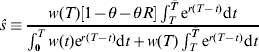
For the case of γ=s, the consumption profile for this individual is monotically increasing across the entire life cycle, except at a possible point of discontinuity (a jump) at the date of retirement. The direction of the jump depends on the level of cumulative savings at the date of retirement, k(T), which is the numerator of (5). We focus on the cases where the jump is negative (i.e., c(T −)|γ=s>c(T +)|γ=s), meaning that we focus on base saving rates that are strictly less than ŝ in our simulation exercises hereinafter, where ŝ is determined by the equations hereinbefore
2.2 Life-cycle/permanent-income consumers
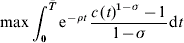
The life-cycle/permanent-income model (augmented for dynamic welfare analysis) is
subject to
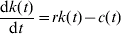


where σ is the inverse elasticity of intertemporal substitution, ρ is the discount rate, and δ is the annual amount that must be deducted from the resources of a life-cycle/permanent-income consumer in order to force his lifetime utility to equal that of a SMarT consumer. This model collapses to the standard model when δ=0, and more will be said about δ later in the paper. The solution to this canonical problem is
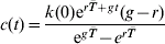
where  is the growth rate of consumption across the life cycle.
3 Welfare analysis – measuring the difference between SMarT and life-cycle/permanent-income behavior
A fundamental assumption that Thaler and Benartzi (Reference Thaler and Benartzi2004) make is that the behavior of some people is not in their own best interest and that such people recognize that their own behavior is suboptimal. This assumption is not unusual and it is supported by evidence. For example, Laibson et al. (Reference Laibson, Repetto and Tobacman1998) survey a body of evidence indicating that the vast majority of Americans believe that they are not saving enough; they say that ‘such systematic, self-acknowledging error contradicts the standard economic model of the maximizing consumer’. Our intention is not to debate this issue, but rather to work within this framework. For example, in terms of the present model setup, we assume that rule-of-thumb consumption is not the result of some underlying optimization process, but rather it is a suboptimal path and the agent would welcome any outside help that brings his behavior more closely in line with life-cycle/permanent-income behavior. In this spirit, we assume that both life-cycle/permanent-income consumers and rule-of-thumb consumers share the same preference structure (CRRA period utility), but the former group follows a path that maximizes lifetime utility, whereas the latter group does not.
Given this assumption we choose δ to be the solution to the following equation

where c p (t; δ) is the consumption profile if the agent follows (15) over the life-cycle, and c s (t; γ) is consumption if the agent follows a SMarT plan as given by (5)–(8). We call δ the ‘income equivalent’, and the associated ‘wealth equivalent’ is
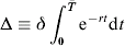
Thus, Δ is the amount of lifetime wealth that must be taken from a life-cycle/permanent-income consumer in order to force his lifetime utility to be the same as the lifetime utility of an otherwise identical SMarT consumer. Although our application is new, this type of metric is conventional in dynamic optimization models and it bears clear resemblance to the usual static theory of consumer welfare. In closed-form, the wealth equivalent is

Let Γ be the set of all γ∊(s, 1] such that Δ<Δ|γ=s (i.e., if Γ=Ø, then SMarT participation cannot improve lifetime utility). To allow for a deeper and dimensionless comparison across alternative parameterizations for cases of Γ≠Ø, we define the ‘efficiency gain’
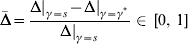
Note that Δ|γ=s is the gap (in dollars) between the lifetime utility of a life-cycle/permanent-income consumer and the lifetime utility of a rule-of-thumb consumer who saves a constant percent, s, of wage income across the entire working period. Note also that Δ|γ=γ* is the gap (again, in dollars) between the lifetime utility of a life-cycle/permanent-income consumer and the lifetime utility of a rule-of-thumb consumer who participates in a SMarT saving plan at rate γ*, where

This rate is the second-best (or constrained) solution to the life-cycle consumption problem, since it maximizes discounted life-cycle utility given that the agent follows a SMarT plan. The main question that we focus on is whether γ* can provide a level of lifetime utility that is close to the level obtained by following the life-cycle/permanent-income rule, and therefore, whether  is large or not (as
 the SMarT plan can perfectly mimic the life-cycle/permanent-income rule; as
 the SMarT plan cannot help at all).
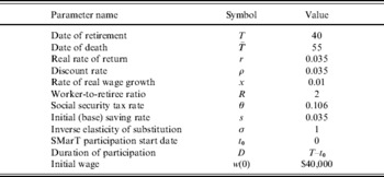
These metrics form the basis of our numerical calculations, and we now select baseline parameter values that we summarize in Table 1. We set T=40 and =55, and we follow recent work in the life-cycle consumption literature by setting r=0.035 (Campbell, Reference Campbell, Campbell, Diamond and Shoven2001; Gourinchas and Parker, Reference Gourinchas and Parker2002; Bullard and Feigenbaum, Reference Bullard and Feigenbaum2007; Feigenbaum, Reference Feigenbaum2007). Furthermore, we follow the convention and set ρ=r. We set x=0.01, because the Bureau of Labor Statistics reports that real wages have grown at about 1% per year in the US over the last decade. The worker-to-retiree ratio is projected to be about 2 within a few decades in the US, and this is the steady state that we examine (Goss, 2005/Reference Goss2006). We choose θ=0.106, since the retirement part of the social security program in the US is funded by payroll taxes equal to 10.6% of earnings, and following the convention the agent pays the full tax in our model (Kotlikoff, Reference Kotlikoff1979; Feldstein, Reference Feldstein1985). We choose 3.5% as a base-saving rate, because this is the average saving rate of people who joined the SMarT plan in the pilot implementations (Thaler and Benartzi, Reference Thaler and Benartzi2004). With these parameters, there will be a drop in consumption at retirement in the absence of SMarT participation, because s<0.099=ŝ. Attanasio (Reference Attanasio, Taylor and Woodford1999)
points out that the balance of the microeconomic evidence indicates σ is very close to 1 in actuality. We assume the individual joins a SMarT plan immediately upon entering the workforce (i.e., t 0=0) and sticks with it until retirement (i.e., D=T−t 0). Finally, the economy-wide wage at t=0 is set to $40,000 for compatibility with the current average wage per worker in the US, but our results are invariant to this assumption. We check the sensitivity of the results to these assumptions hereinafter.
Baseline parameter values

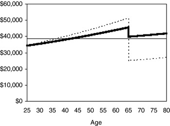
We find that γ*=0.32 at the baseline parameter values. Figure 1 shows consumption over the life cycle for a life-cycle/permanent-income consumer (the thin solid line), a SMarT consumer who has opted to use the SMarT rate of 32% (the thick solid line), and a rule-of-thumb consumer who does not participate in the SMarT plan meaning γ=s=0.035 (the dashed line). At this parameterization, the SMarT plan clearly leads to a smoother consumption profile than with no SMarT plan in force. The wealth equivalents are Δ|s=0.035, γ=0.32=$2, 732 and Δ|γ=s=0.035=$13, 700. That is, the loss to lifetime wealth associated with following a SMarT plan (with a base saving rate of 3.5% and a SMarT rate of 32%) rather than the life-cycle/permanent-income rule is $2, 732, whereas the loss to lifetime wealth associated with saving a fixed fraction of all wages across the life cycle (i.e., γ=s=0.035) rather than following the life-cycle/permanent-income rule is $13, 700. Hence, the efficiency gain is

which means that the SMarT plan takes a rule-of-thumb agent 80% closer to the unconstrained optimum. Apparently, the SMarT plan can be a significant improvement over a flat and low saving rate.
Life-cycle consumption for three consumers

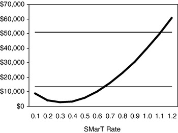
One common concern is that the SMarT plan is so popular and powerful that participants will accidentally oversave. In Figure 2, we plot the wealth equivalent, Δ, for various values of γ ranging from 0.1 to 1.2 (this upper bound on γ is above what we generally consider in our simulations). The thick line corresponds to the SMarT plan (i.e., it is Δ|s=0.035, γ>s), and the lower thin flat line corresponds to no SMarT plan (i.e., Δ|γ=s=0.035). The SMarT plan is optimized at γ=0.32, as this is precisely the minimum of Δ|s=0.035, γ>s. However, the SMarT plan will improve lifetime utility above that of simple saving only if Δ|s=0.035, γ>s<Δ|γ=s=0.035, and this occurs if the SMarT rate is 66% or less. The SMarT plan becomes increasingly inferior to a simple saving plan as the SMarT rate increases beyond 66%. Finally, the upper thin flat line is the wealth equivalent for a hand-to-mouth consumer who never saves anything (i.e., Δ|γ=s=0). Our computations show that this line intersects the wealth equivalent when the SMarT rate is about 1.1, suggesting an overly aggressive SMarT rate can even make the agent worse off than that of hand-to-mouth behavior. We do not necessarily interpret this as a weakness in the SMarT plan itself, but it rather highlights that care must be taken to determine the appropriate execution of the plan.
The wealth equivalent: measuring the deviation from life-cycle/permanent-income behavior

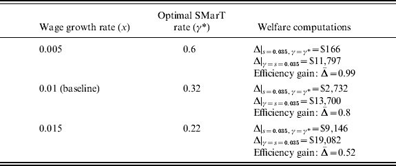
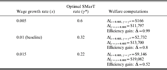
The rate of real wage growth plays a key role in our analysis, because SMarT saving is tied to wage increases. We therefore test the robustness of our findings to this parameter. Recall the optimal SMarT rate, γ*, is 32% if the rate of real wage growth is 1%. If we consider a lower rate of wage growth, say 0.5%, then the optimal SMarT rate increases to 60% with a corresponding wealth equivalent of $166. Moving in the other direction, if the rate of wage growth is 1.5%, then the optimal SMarT rate is 22% with a wealth equivalent of $9,146. These results are summarized in Table 2.
Sensitivity of efficiency gain to rate of real wage growth
Note: =(Δ|γ=s−Δ|γ=γ*)/Δ|γ=s.
There are a few interesting lessons in Table 2. First, the optimal SMarT rate is inversely related to the rate of wage growth, and seemingly small changes in the rate of wage growth can produce large changes in the optimal SMarT rate. Second, the efficiency gain, , associated with optimal usage of the SMarT plan (when γ=γ*) is also inversely related to the rate of real wage growth. And third, over the range of wage growth rates and other parameters that we have considered, the efficiency gain from SMarT participation is always large.
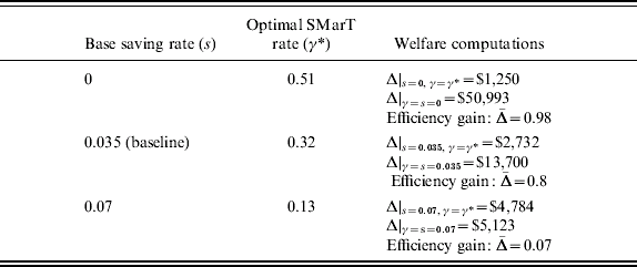
Another variable that plays a key role in our calculations is the base saving rate, s. In Table 3 we show the sensitivity of our baseline estimate of the efficiency gain to changes in the base saving rate. There are a number of concepts in Table 3 that merit our attention. First and the most obvious, the optimal SMarT rate is inversely related to the base saving rate. Second, the wealth equivalent is huge when the agent is a hand-to-mouth consumer with a base saving rate set at zero (Δ|γ=s=0=$50,993), and the efficiency gain from SMarT participation can be surprisingly large for such consumers (=0.98). Nearly all of the welfare cost from hand-to-mouth behavior is erased through SMarT participation if the agent can truly commit to the SMarT plan. Third, for individuals with higher base saving rates, say 7%, the wealth equivalent is already relatively small Δ|γ=s=0.07=$5,123, and there is not a lot the SMarT plan can do to help (=0.07).
Sensitivity of efficiency gain to base saving rate
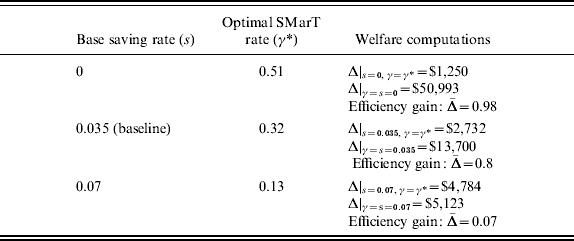
Note: =(Δ|γ=s−Δ|γ=γ*)/Δ|γ=s.
4 The effect of family-size dynamics on the value of SMarT participation
We now extend the model to the realistic case where parents must provide for the consumption needs of dependent children living in the home. This extension is likely to be especially important for uneducated people, who generally have a larger number of children (Haliassos and Reiter, Reference Haliassos and Reiter2005). Let c(t) now represent total household consumption of a married couple and their children with period utility following Haliassos and Reiter (Reference Haliassos and Reiter2005),  , where n(t) is the effective household size. Let n(t)=2+κn c(t), where n c(t) is the number of children at time t and κ=0.4. In the US, family size typically reaches a peak when the household head is around 45 years of age (Attanasio et al. Reference Attanasio, Banks, Meghir and Weber1999), and children are often spaced a few years apart rather than all at once. To capture these key facts, we use a stylized, bell-shaped, continuously differentiable function n c(t)=n maxcΦ(t), where n maxc is the maximum number of children present at home and where
 with Φ(t)⩽1 (given λ>0). The strict inequality holds for all t, except at t=α−1, which is the point at which
 reaches a peak (i.e.,
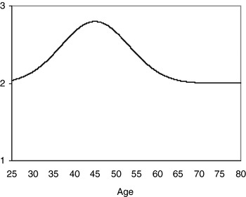
 ). Clearly then, Φ(α−1)=1 and n(α−1)=2+κn maxc. If n maxc=0, the model degenerates to the baseline model from above. To calibrate family-size dynamics to the data which suggests a peak in n(t) at t=20 (i.e., age 45 given that time zero corresponds to age 25), we choose α=1/20, and we set λ=3 to ensure that the tails of Φ(t) are slim near the start and the end of the working period. This captures the realistic idea that there are viturally no children at home at the start or at the end of the working phase. Figure 3 plots n(t) for the case of n maxc=2.
Effective household size over the life cycle

If the household behaves according to the life-cycle/permanent-income rule, then it chooses consumption at any time t according to
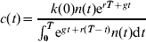
or, in growth terms the Euler equation is 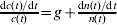 . For the baseline case with g=0, this clearly implies that the optimal consumption path increases during the early part of the working years when the size of the household is growing, and decreases during the latter part of the working years when the size of the household is shrinking as children become independent and leave the home. Furthermore, α−1=arg maxt∊[0,
 ]{c(t)|g=0}.
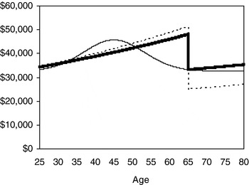
As before, we are interested in those consumers who do not follow such a life-cycle/permanent-income plan, but instead follow a simple rule of thumb in which a constant (and potentially low) fraction of wage income is saved. Such rule-of-thumb consumers ignore the optimality condition that requires consumption to be maximized when the number of dependents in the home is maximized, and so the question that we address is whether it pays to be SMarT even when family-size dynamics are included? The answer to this question is not obvious since it appears that there are competing forces at work here. On the one hand, a SMarT consumer saves more for retirement than an otherwise equivalent rule-of-thumb consumer, which may consequently lead to a higher level of lifetime utility for the SMarT consumer if the rule-of-thumb consumer saves at a low rate and accumulates too little for retirement. On the other hand, the SMarT consumer tends to have a flatter consumption profile than a simple rule-of-thumb consumer, and a flat consumption profile is not particularly desirable from a lifetime utility perspective because the life-cycle/permanent-income consumption profile is hump-shaped. Hence, it is a quantitative question of whether or not the SMarT plan improves utility for this case. We find that this second effect is non-trivial and somewhat erodes the advantage of the SMarT plan. For example, with n maxc=2 (corresponding to a family of 4 comprised of 2 adults and 2 children) and with all other parameters set at baseline values, the optimal SMarT rate is 20% with a corresponding efficiency gain of 39%. This is half of the baseline estimate of =0.8 with no family-size dynamics included. Figure 4 plots consumption profiles for simple rule-of-thumb, SMarT, and life-cycle/permanent-income consumers.
Life-cycle consumption for three consumers with family-size dynamics and immediate SMarT entry

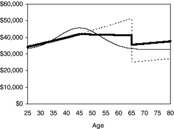
While this appears to suggest that family size dynamics can dampen the efficiency gains from SMarT participation, this estimate is biased against the SMarT plan because we have assumed that the agent joins a SMarT plan immediately upon joining the work force. A more strategic use of the SMarT plan would involve delayed entry, at say age 45, so that the increased saving effort is synchronized with the shrinking number of dependent children in the home (thus roughly mimicking some of the qualitative properties of the life-cycle/permanent-income consumption rule). Such a strategy should be a significant improvement over the simple rule of thumb which implies that the agent's consumption continues to increase exponentially throughout the entire working period even though children may have already left home. For example, Figure 5 shows the case where t 0=20 to capture SMarT enrollment at age 45 with all other parameters set to baseline values. Now the optimal SMarT rate is 97% and the efficiency gain is =0.69, which is much bigger than with immediate entry into a SMarT plan and nearly as big as the baseline model without children (=0.8). These results suggest that including children in the analysis affects the optimal timing of entry into a SMarT plan, where late entry is especially advantageous in order to protect against over saving during the middle years when consumption spending is highly productive at home.
Life-cycle consumption for three consumers with family-size dynamics and delayed SMarT entry

5 The employer's problem: default choice under saving-rate heterogeneity and participation uncertainty
In this section, we turn to some of the important issues faced by an employer who is considering the implementation of a SMarT plan for employees. Specifically, we consider the case of an altruistic employer who wants to help employees attain the highest possible levels of lifetime utility; yet, choosing a default SMarT rate for the plan is not straightforward because employees are heterogeneous with respect to their base saving rates and with respect to whether they will stick with the plan. Let us state the problem formally.
Consider a forward-looking, altruistic employer who is in charge of a collection of J rule-of-thumb employees indexed by j∊{1, 2, …, J}, who differ in their base saving rate s j=s+εj, where εj∊{ε1, ε2, …, εJ} with the restrictions ε1<ε2<…<εJ, ε1⩾−s and εJ<ŝ−s. The employer presently has not offered a SMarT program but is about to make one available to the employees. The goal of the employer is to choose a single SMarT saving rate as a default setting for employees, while still allowing employees the right to opt out of the SMarT program and return to baseline saving levels at any time. However, based on the evidence in behavioral science concerning inertia and the importance of defaults, the employer believes that some employees may stick with the default setting, and therefore, the employer must be careful with the default selection.
At t=0 the employer implements a SMarT program for employees (so t 0=0 by assumption), and without loss of generality, we let the duration of participation D j take a binary form

for p j∊{p 1, p 2, …, p J}. The employer maximizes the expected utility of employees by choosing
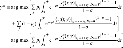
where the last line follows from the fact that  . In the selection of γ, the employer clearly places the most weight on those employees who are most likely to stick with the SMarT program. Other things equal, the employer also places more weight on the lower savers since the SMarT plan generates larger gains for them compared to higher savers (recall Table 3). These forces may work together, in the opposite direction, or they may be unrelated depending on the nature of the correlation between p j and εj. So, we break out into three stylized cases of the model.
5.1 Case 1. pj= <1 for j⩽j* and pj=1 for j>j*
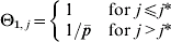
Let j* be the threshold employee. He and other employees j<j* with saving rates s j<s j* have a probability  <1 of sticking with the SMarT program. All other employees j*+1, j*+2, …, J with saving rates s j>s j* will stick with the plan with certainty. This case captures a common concern that employees who initially have low saving rates are less likely to stick with the SMarT program compared to those who initially have high saving rates. Hence the problem reduces to

where Θ1, j is an indicator variable
5.2 Case 2. pj=1 for j⩽j* and pj=<1 for j>j*
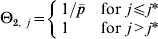
This is the reverse of Case 1, because now it is those employees who initially have high saving rates that are less likely to stick with the SMarT program. This could be true if those with high initial saving rates feel that they are already saving enough.Footnote 4 The problem for this case becomes

where Θ2, j is an indicator variable
5.3 Case 3. pj=∊(0, 1] for all j
This is a simple way to capture the possibility that the likelihood of sticking with the SMarT program is unrelated to the initial saving rates of employees. The employer's problem is independent of p j

5.4 Quantitative results
To make progress on the numerical computations, we set J=2 to reduce the dimensions of the problem while still preserving the action that comes from heterogeneity (here j*=1). Let us continue to suppose that the average saving rate is s=0.035. Actually, we can either assume that there are literally only two employees or that there are many employees but only two types; either interpretation will suffice.
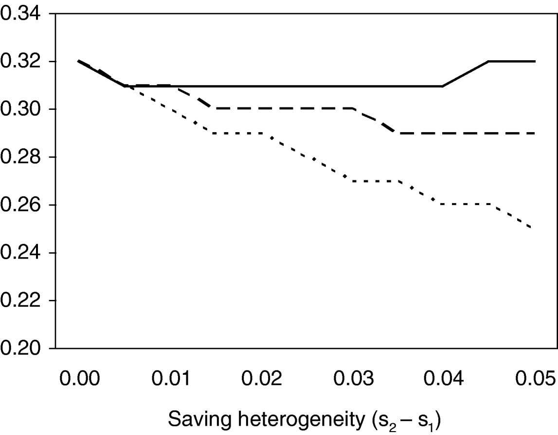
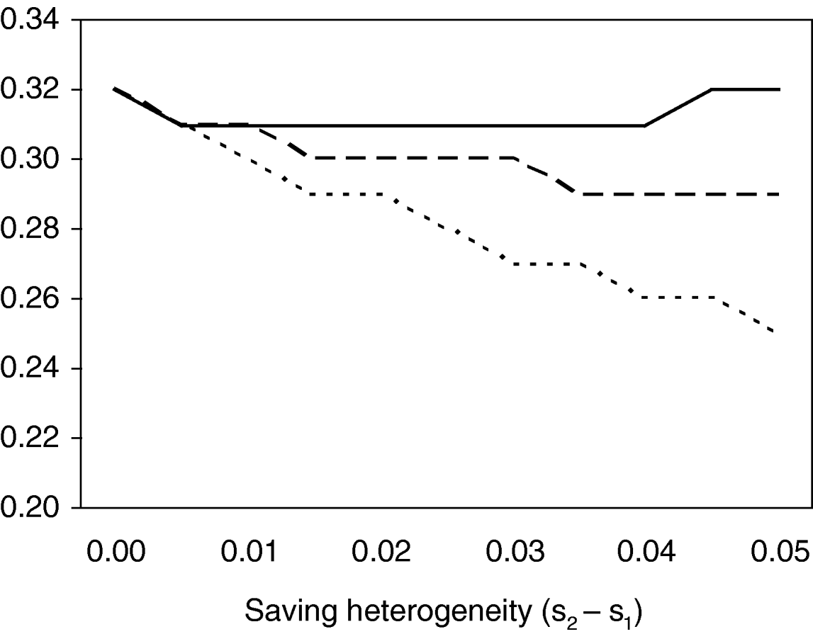
CASE 1. Assume the employee with the higher saving rate (j=2) has a 100% probability of sticking with the SMarT plan (p 2=1), while the low saver has a probability less than one (p 1<1). In Figure 6, we plot the optimal SMarT default rate from the employer's perspective, as a function of the degree of heterogeneity in saving rates (i.e., s 2−s 1) where heterogeneity increases as we move from left to right on the graph. The solid line corresponds to the case where p 1=0.75, the dashed line corresponds to p 1=0.5, and the dotted line corresponds to p 1=0.25. Clearly, heterogeneity in saving rates has a larger effect on the optimal default rate when there is also a greater degree of heterogeneity in the likelihood of participation. For example, in the case when the likelihood of participation among low savers is relatively high (the solid line) and is therefore closer to the likelihood of participation among high savers, the effect of heterogeneity in saving rates on the optimal SMarT default rate is almost non-existent for the parameter space that we consider. On the other hand, the effect of heterogeneity in saving rates on the optimal SMarT default is more pronounced when participation is unlikely among those with low saving rates (i.e., when there is more heterogeneity along the participation dimension). It is almost always the case in Figure 6 that an increase in the degree of saving-rate heterogeneity tends to reduce the optimal SMarT default rate.
Optimal SMarT default when low-savers are less likely to participate: under saving heterogeneity and participation uncertainty
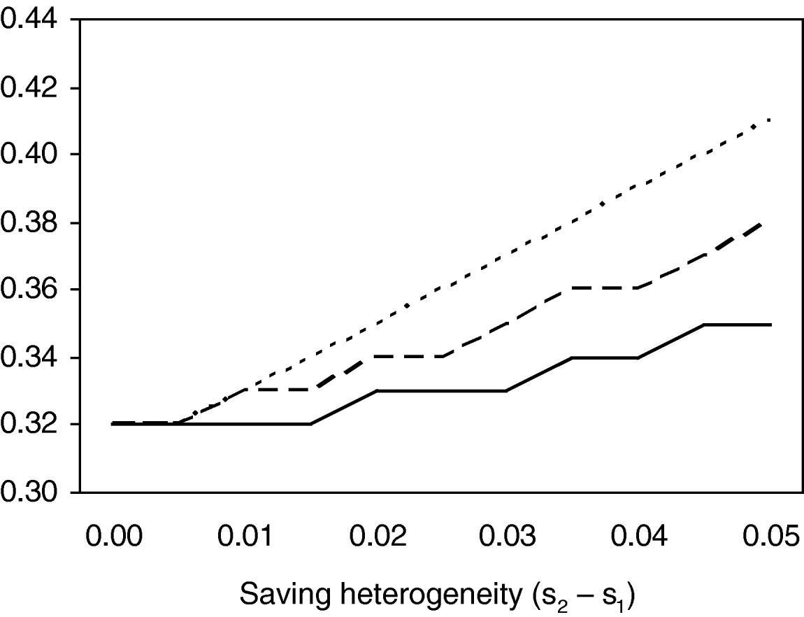
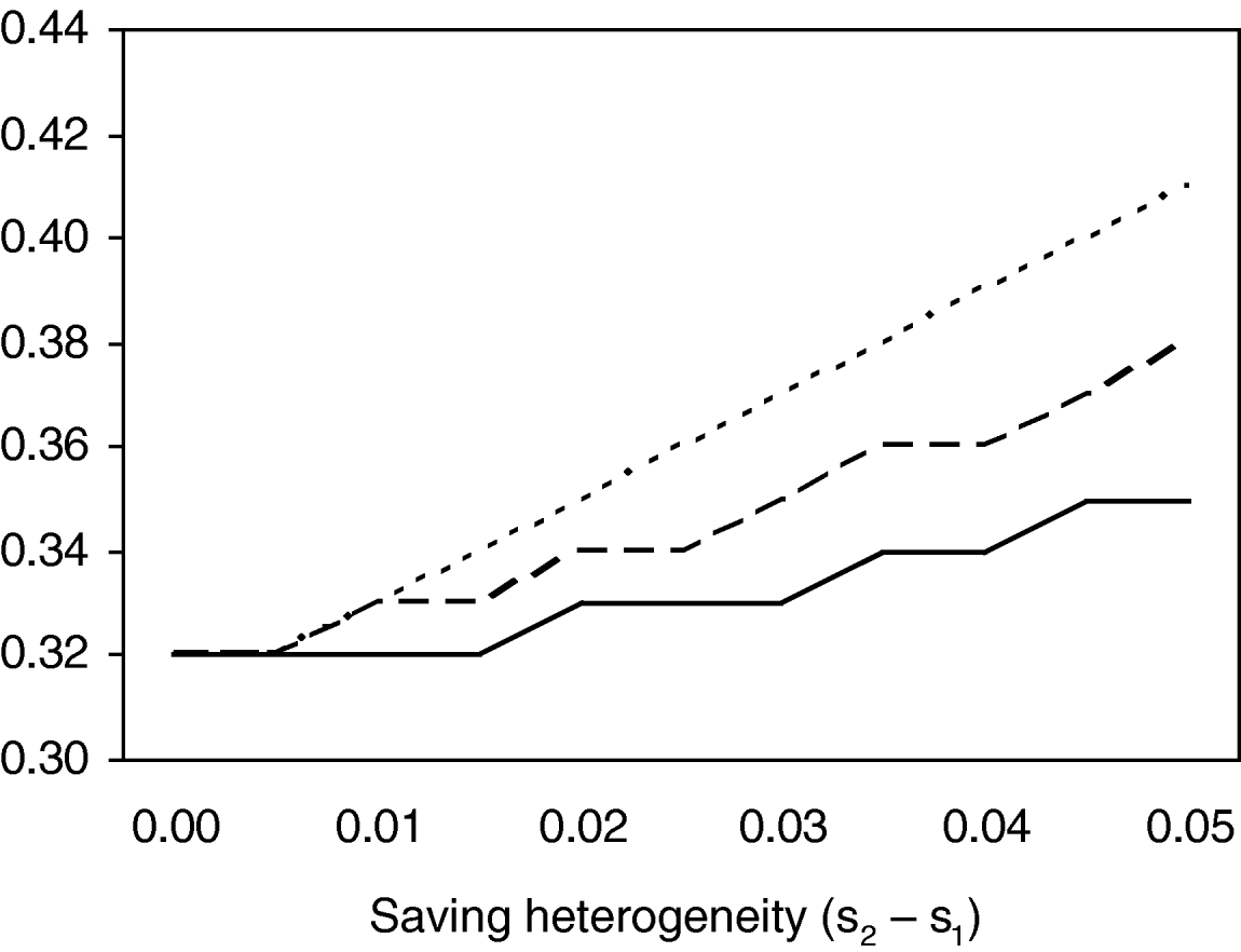
CASE 2. We now assume that the employee with a higher saving rate (j=2) has a probability of participation p 2<1 while the low saver has a probability p 1=1. In Figure 7, we plot the optimal SMarT default rate from the employer's perspective, as a function of the degree of heterogeneity in saving rates (s 2−s 1). The solid line corresponds to the case where p 2=0.75, the dashed line corresponds to p 2=0.5, and the dotted line corresponds to p 2=0.25. Again, heterogeneity in saving rates has a larger effect on the optimal default rate when there is also a greater degree of heterogeneity in the likelihood of participation. In the case where the likelihood of participation among high savers is relatively high (the solid line), the effect of heterogeneity in saving rates on the optimal SMarT rate is not nearly as strong as in the case where the likelihood of participation among high savers is low (the dotted line). This is seen by noting that the dotted line is the steepest and the solid line is the flattest in Figure 7.
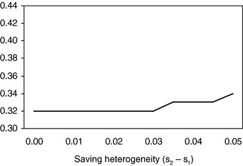
CASE 3. Here we examine the pure effect of saving-rate heterogeneity since all employees have an equal probability of participation. At our baseline parameterization, there is a positive relationship between the degree of heterogeneity in the saving rate (holding the mean fixed at 3.5%) and the optimal SMarT default rate. This is evident in Figure 8, yet we clearly see that the effect of such a mean-preserving increase in saving heterogeneity is modest in isolation; it is the interaction of saving heterogeneity and participation uncertainty that is driving most of the action depicted in Figures 6 and 7. It is also interesting that the pure effect of saving-rate heterogeneity on the optimal SMarT default rate is positive, but that this result does not necessarily continue to hold when mixed with heterogeneity in participation uncertainty. The pure effect of saving-rate heterogeneity is amplified in the case where those with high saving rates are least likely to participate, and the pure effect of saving-rate heterogeneity is dampened or even reversed for the case where those with low saving rates are least likely to participate.
Optimal SMarT default when high-savers are less likely to participate: under saving heterogeneity and participation uncertainty
Optimal SMarT default with equal participation across saver types: under saving heterogeneity

7 The employer's problem: default choice under risk-taking heterogeneity
We now consider the case with uncertainty in the rate of return to saving, in which some employees avoid risk and others look for it. Again, there is a collection of J rule-of-thumb employees indexed by j∊{1, 2, …, J}. There is a stylized risky asset and a safe asset, and the expected return on the risky asset is higher than the return on the safe asset. At t=0, the employer implements a SMarT program for employees (so t 0=0 by assumption), where Ξj is an indicator variable for risk taking

The effective rate of return during the working period t∊[0, T] for employee j is r j(t)=r+Ξjξj, where ξj is a heterogeneous disturbance that depends on the level of risk taken on by employee j

The restriction χj>1/2 together with the mapping  for all ν∊핉+ captures the risk-reward tradeoff. The share of risk-taking employees is
 and we assume that all employees hold safe assets during retirement.
Abstracting from participation uncertainty (D=T for all j), the annuity for the risk-takers is
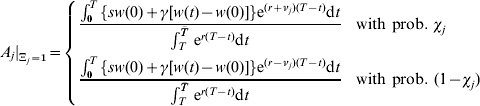
and  is given by (5) as usual (with t 0=0 and D=T). Let us assume that employees j⩽j ν are risk-avoiders with Ξj=0, and employees j>j ν are risk-takers with Ξj=1.
The altruistic employer maximizes the expected utility of employees by choosing
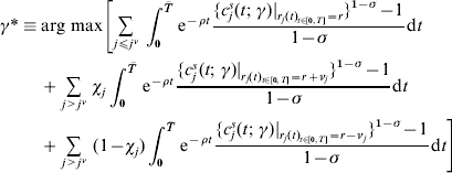
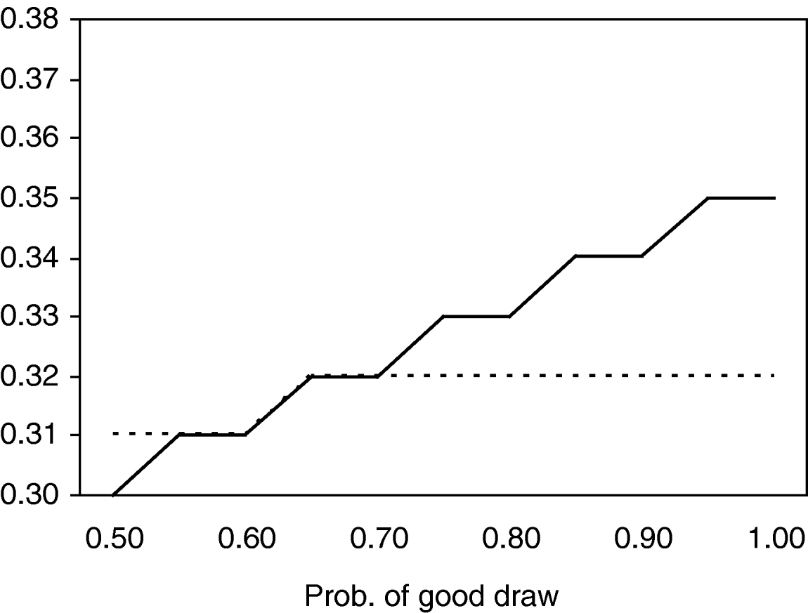
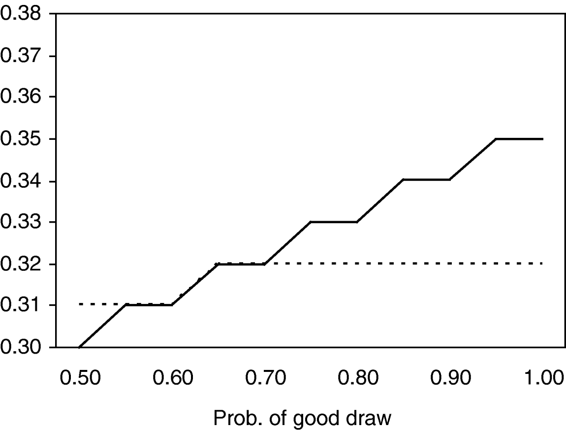
Turning to the quantitative results, let us simplify by assuming νj=0.03 for all j>j ν. In Figure 9, we show how the optimal SMarT default is related to the degree of risk experienced among the risk-takers. As we move from left to right (i.e., as χ increases), the expected return on the risky investment increases, and this has a positive effect on the optimal SMarT rate in two hypothetical ‘bookend’ cases: the solid line corresponds to the case where 90% of employees are risk-takers, and the dotted line is the case where 10% are risk-takers. The reason why these lines are upward sloping is not obvious. On the one hand, it might be expected that if the likelihood of a bad draw is high (χ is low), then a high SMarT default would be optimal in order to ensure that the risk-taking employees have sufficient assets at retirement; but on the other hand, a low default prevents the risk-taking employees from dumping too much money into a savings account that has a high probability of earning a low return. It appears that the second effect dominates under the space of parameters considered here.
Optimal SMarT default with heterogeneity in risk taking
7 Debt accumulation as a response to SMarT participation
Suppose employees technically stick with the SMarT program but sometimes borrow against the flow of SMarT saving, thus counteracting participation at that point in time. Let us consider I intervals of time t∊[αi, βi] for i∊{1, 2, …, I}, given βi>αi and αi+1>βi, where employees borrow the flow ζiγ[w(t)−w(t 0)] given ζi∊[0, 1], which accumulates at rate r ζ⩾r. We further assume  for any i. Note that the flow of borrowing can vary over time for two reasons: first, it may be the case that ζi≠ζi+1; and secondly, wages are growing. We assume α1⩾t 0=0, βI⩽T=D, and that all debt accumulation is paid off at the date of retirement. The remaining net private assets are annuitized over the retirement period

Consumption during the working period is given by


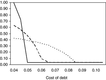
Let us abstract from the frequency dimension and consider the special case of I=1, α=0, and β=T, where ζ governs the intensity of borrowing and r ζ the cost of borrowing. Figure 10 plots the optimal SMarT rate against the cost of debt, given that the employee responds to SMarT participation by borrowing at a rate that is at least as high as the rate of return to saving. The solid line is the case where the flow of borrowing is 75% as large as SMarT saving (ζ=0.75). The dashed line is the case where borrowing is 50%, and the dotted line is the case of 25%.
Optimal SMarT rate when consumers borrow against SMarT saving

While it might be tempting to anticipate that the optimal SMarT rate is a decreasing function of the magnitude of the borrowing response, ζ, this is clearly not always the case. When the cost of debt is the same or slightly higher than the return to saving, then the optimal SMarT rate is highest when the degree of borrowing is greatest. Note that the solid line lies above the dashed line, which in turn lies above the dotted line. However, as the cost of debt gets increasingly larger than the return to saving, the optimal SMarT rate plunges very rapidly when the borrowing response is highest. Convergence to an optimal SMarT rate of 3.5% (i.e., no SMarT program at all) occurs for all the three cases in Figure 10, but the rate of convergence clearly depends on the intensity of borrowing. This leads to intersections, and therefore reversals of the relationship between the borrowing parameter, ζ, and the optimal SMarT rate. There are two competing forces that cause this reversal. When the borrowing response is high, then a low SMarT rate will keep the employee from accumulating too much high-cost debt; however, it is also the case that when the borrowing response is high, the employee needs a high SMarT saving rate in order to achieve a target level of net saving at retirement. The second effect can dominate if the cost of borrowing is the same or slightly higher than the return on saving.
8 Conclusion
Using rigorous neoclassical tools for dynamic welfare analysis, we have attempted to quantify the value of the prescriptive SMarT plan relative to the normative life-cycle/permanent-income model. In addition to being a tremendously popular plan that encourages people to save more for retirement, our quantitative-theoretic analysis tends to support the SMarT plan as a decent first approximation to the normative ideal. We have also studied some of the important issues relating to the optimal implementation of a SMarT plan, from the perspective of an altruistic employer. Our hope is that our analysis of the ‘employer's problem’ may be useful in providing broad insights and by highlighting tradeoffs concerning the implementation of a SMarT default on saving plans for a heterogeneous pool of employees.
One potential area for future research is the study of pre-commitment devices during the retirement stage of the life cycle. The SMarT plan acts as a pre-commitment device during the working years (as do tax-advantaged saving vehicles such as 401(k)s and IRAs by imposing penalties on early withdrawals). These plans and vehicles aim to help people accumulate enough savings to afford a comfortable retirement, yet the issue of how to pre-commit retirees to follow an optimal withdrawal plan during the payout stage also seems important especially in the face of mortality risk, health shocks, a risky financial environment, and the absence of a well-defined market for lifetime annuities. With over 50 million baby boomers on the verge of retirement, the question of optimal asset depletion may very well be just as important as how to help people save for retirement.
The Save More Tomorrow™ (or SMarT) plan is a registered trademark of Richard Thaler and Shlomo Benartzi. We thank Mike Orszag and an anonymous referee for their helpful comments.