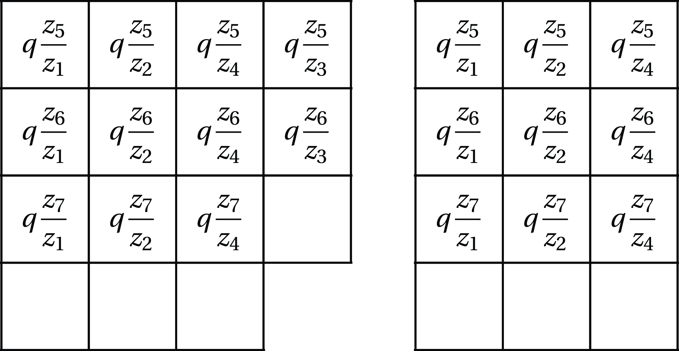
1. Introduction
Inspired by the science fiction conjecture proposed by Bergeron and Garsia [Reference Bergeron and GarsiaBG99], we examine Macdonald intersection polynomials, which are conjectured to be equal to the bigraded Frobenius characteristic of the intersection of Garsia–Haiman modules. To provide a comprehensive overview of the primary results, we discuss the historical context and background of Macdonald polynomials, the shuffle theorem, and the science fiction conjecture.
1.1 Macdonald polynomials
In his seminal paper [Reference MacdonaldMac88], Macdonald introduced the Macdonald
 $P$
-polynomials
 $P_\mu [X;q,t]$
, which can be seen as a
 $(q,t)$
generalization of Schur functions. Macdonald polynomials specialize to important families of symmetric functions such as Jack symmetric functions and Hall–Littlewood polynomials. They have been widely researched and have numerous applications in representation theory, algebraic geometry, and mathematical physics, among other fields. Garsia and Haiman introduced a combinatorial variant of Macdonald polynomials called the modified Macdonald polynomial, which is defined by the plethystic substitution of the Macdonald
 $J$
-polynomial of [Reference MacdonaldMac88]:
 \begin{equation*} \widetilde {H}_\mu [X;q,t] = t^{n(\mu )}J_\mu \bigg[\dfrac {X}{1-t^{-1}};q,t^{-1}\bigg]. \end{equation*}
One of the most fascinating questions surrounding Macdonald polynomials was the Macdonald positivity conjecture, which deals with the Schur positivity of the modified Macdonald polynomials.
In 1993, Garsia and Haiman introduced the Garsia–Haiman module
 $V_\mu$
associated to a partition
 $\mu \vdash n$
as the subspace in
 $\mathbb {C}[\mathbf {x}_n,\mathbf {y}_n]:=\mathbb {C}[x_1,\dots ,x_n,y_1,\dots ,y_n]$
spanned by partial derivatives of the ‘generalized’ Vandermonde determinant
 $\Delta _\mu$
associated to
 $\mu$
(see [Reference Garsia and HaimanGH93, Reference Garsia and HaimanGH96b]). They expected the Garsia–Haiman modules to serve as a representation-theoretic model for the modified Macdonald polynomials. More specifically, they conjectured that
 \begin{equation*} \mathrm {grFrob}(V_\mu ;q,t) = \widetilde {H}_\mu [X;q,t], \end{equation*}
where
 $\mathrm {grFrob}$
denotes the bigraded Frobenius characteristic. This conjecture is known as the
 $n!$
-conjecture, which in particular implies that
 $\dim V_\mu = n!$
. Haiman [Reference HaimanHai01] ultimately proved the
 $n!$
-conjecture by utilizing the geometry of the Hilbert scheme of
 $n$
points in a plane, thereby confirming the Macdonald positivity conjecture. However, his proof does not offer a combinatorial formula for the Schur coefficients, the
 $(q,t)$
-Kostka polynomials
 $\widetilde {K}_{\lambda ,\mu }(q,t)$
, which remains a significant open problem.
The celebrated result of Haglund, Haiman, and Loehr made important progress in giving a combinatorial formula for the modified Macdonald polynomials. For a partition
 $\mu$
of
 $n$
, the Haglund–Haiman–Loehr formula [Reference Haglund, Haiman and LoehrHHL05] gives
 \begin{equation} \widetilde {H}_\mu [X;q,t] = \sum _{w \in \mathfrak {S}_n} q^{\mathrm {inv}_\mu (w)} t^{\mathrm {maj}_\mu (w)} F_{\mathrm {iDes}(w)}. \end{equation}
Here, the sum is over all permutations of
 $[n]$
, the functions
 $\mathrm {inv}_\mu$
and
 $\mathrm {maj}_\mu$
are certain statistics associated to a partition
 $\mu$
, and
 $F$
is the (Gessel’s) fundamental quasisymmetric function.
1.2 The nabla operator and shuffle theorem
The nabla operator
 $\nabla$
, introduced by Bergeron and Garsia, is an operator acting on symmetric functions with coefficients in
 $\mathbb {Q}(q,t)$
. It is an eigen-operator for the modified Macdonald polynomials:
 \begin{equation*} \nabla \widetilde {H}_\mu [X;q,t] = T_\mu \widetilde {H}_\mu [X;q,t] , \end{equation*}
where
 $T_\mu :=\prod _{(i,j)\in \mu }t^{i-1}q^{j-1}$
. Remarkably, the nabla operator is closely related to the diagonal coinvariant algebra
 $\mathrm {DR}_n$
, which is defined as
 \begin{equation*} \mathrm {DR}_n:=\mathbb {C}[\mathbf {x}_n,\mathbf {y}_n]/\langle \mathbb {C}[\mathbf {x}_n,\mathbf {y}_n]^{\mathfrak {S}_n}_+\rangle , \end{equation*}
where the symmetric group
 $\mathfrak {S}_n$
acts on the polynomial ring
 $\mathbb {C}[\mathbf {x}_n,\mathbf {y}_n]$
by the diagonal action. Haiman [Reference HaimanHai02] proved the
 $(n+1)^{n-1}$
-conjecture, which asserts that
 $\dim \mathrm {DR}_n = (n+1)^{n-1}$
, and provided a formula for the bigraded Frobenius character of
 $\mathrm {DR}_n$
,
 \begin{equation*} \mathrm {grFrob}(\mathrm {DR}_n) = \nabla e_n, \end{equation*}
where
 $e_n$
is the
 $n$
th elementary symmetric function.
The shuffle conjecture, proposed by Haglund et al. [Reference Haglund, Haiman, Loehr, Remmel and UlyanovHHLRU05], anticipates a combinatorial formula
 \begin{equation*} D_n[X;q,t]:=\sum _{(\pi ,w) \in \mathrm {Park}_n}t^{\mathrm {area}(\pi )}q^{\mathrm {dinv}(\pi ,w)} F_{\mathrm {iDes}(w)} \end{equation*}
for
 $\nabla e_n$
. Here, the sum is over all parking functions
 $(\pi ,w)$
of length
 $n$
, and the functions
 $\mathrm {area}$
and
 $\mathrm {dinv}$
are statistics associated to each parking function. We refer to the generating function
 $D_n[X;q,t]$
as the shuffle formula. Carlsson and Mellit [Reference Carlsson and MellitCM18] eventually proved the shuffle conjecture by introducing the Dyck path algebra, which is closely related to the double affine Hecke algebra. Since then, numerous aspects of the nabla operator and its generalizations, including their combinatorial formulas, have been extensively investigated [Reference HaimanHai02, Reference MellitMel18, Reference Blasiak, Haiman, Morse, Pun and SeelingerBHMPS21, Reference Carlsson and MellitCM21, Reference Blasiak, Haiman, Morse, Pun and SeelingerBHMPS23, Reference D’Adderio and MellitDM22].
1.3 Science fiction conjecture and Macdonald intersection polynomials
Prior to Haiman’s proof of the Macdonald positivity conjecture, Bergeron and Garsia proposed a conjectural combinatorial approach to constructing a basis for
 $V_\mu$
in [Reference Bergeron and GarsiaBG99], known as the science fiction conjecture. Specifically, they presented series of conjectures concerning the intersection of Garsia–Haiman modules. To elaborate, for a partition
 $\mu \vdash n+1$
, let
 $\mu ^{(1)},\dots ,\mu ^{(k)}\subseteq \mu$
be
 $k$
distinct partitions such that
 \begin{equation*} |\mu /\mu ^{(1)}|=\cdots =|\mu /\mu ^{(k)}|=1. \end{equation*}
Let
 $T^{(i)}:= T_{\mu ^{(i)}}$
for
 $i=1,\dots ,k$
. The science fiction conjecture suggests the following:
-
(1) the bigraded Frobenius characteristic of the intersection of the modules
 $\bigcap _{i=1}^{k} V_{\mu ^{(i)}}$
is given byand
\begin{equation*} \mathrm {I}_{\mu ^{(1)},\dots ,\mu ^{(k)}}[X;q,t]:=\sum _{i=1}^{k} \bigg (\prod _{j\neq i}\dfrac {T^{(j)}}{T^{(j)}-T^{(i)}}\bigg )\widetilde {H}_{\mu ^{(i)}}[X;q,t]; \end{equation*}
-
(2) the dimension of
$\bigcap _{i=1}^{k} V_{\mu ^{(i)}}$
is
$n!/k$
.


We refer to the symmetric function
 $\mathrm {I}_{\mu ^{(1)},\dots ,\mu ^{(k)}}[X;q,t]$
as the Macdonald intersection polynomial and the second assertion as the
 $n!/k$
-conjecture. In an earlier paper [Reference Kim, Lee and OhKLO22], the authors examined Macdonald intersection polynomials for two partitions (when
 $k=2$
), which was considered in Butler’s conjecture [Reference ButlerBut94]. More specifically, the authors provided a (positive) combinatorial formula for
 $\mathrm {I}_{\mu ^{(1)},\mu ^{(2)}}[X;q,t]$
that is analogous to the Haglund–Haiman–Loehr formula (1.1). In this paper, we delve deeper into the properties of Macdonald intersection polynomials
 $\mathrm {I}_{\mu ^{(1)},\dots ,\mu ^{(k)}}[X;q,t]$
.
1.4 Main results
We state the first main result of this paper. A direct implication of assertions (b) and (c) of Theorem 1.1 is a new proof of the shuffle theorem.
Theorem 1.1.
Given a partition
 $\mu \vdash n+1$
, let
 $\mu ^{(1)},\dots ,\mu ^{(k)}\subseteq \mu$
be
 $k$
distinct partitions such that
 \begin{equation*} |\mu /\mu ^{(1)}|=\cdots =|\mu /\mu ^{(k)}|=1. \end{equation*}
The Macdonald intersection polynomial
 $\mathrm {I}_{\mu ^{(1)},\dots ,\mu ^{(k)}}[X;q,t]$
satisfies the following.
-
(a) For
$m\lt k-1$
, we have
\begin{equation*} e_{n-m}^\perp \mathrm {I}_{\mu ^{(1)},\dots ,\mu ^{(k)}}[X;q,t]=0. \end{equation*}
-
(b) We have
In particular,
\begin{equation*} \dfrac {1}{T_{\bigcap _{i=1}^k \mu ^{(i)}}}e_{n+1-k}^\perp \left (\mathrm {I}_{\mu ^{(1)},\dots ,\mu ^{(k)}}[X;q,t]\right ) = \nabla e_{k-1}. \end{equation*}
$e_{n+1-k}^\perp \mathrm {I}_{\mu ^{(1)},\dots ,\mu ^{(k)}}[X;q,t]$
does not depend on the partitions
$\mu ^{(1)}, \dots , \mu ^{(k)}$
and on
$\mu$
(up to a constant).
-
(c) We have
\begin{equation*} \dfrac {1}{T_{\bigcap _{i=1}^k \mu ^{(i)}}}e_{n+1-k}^\perp \left (\mathrm {I}_{\mu ^{(1)},\dots ,\mu ^{(k)}}[X;q,t]\right ) = D_{k-1}[X;q,t]. \end{equation*}


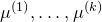


Here,
 $e_n^\perp$
denotes the adjoint operator to the multiplication by
 $e_n$
with respect to the Hall inner product.
Corollary 1.2 [Shuffle theorem, Reference Carlsson and MellitCM18]. We have
 $\nabla e_n=D_{n}[X;q,t]$
.
We refer to the equation in Theorem 1.1(a) as the vanishing identity. The second and the third assertions give miraculous relationships between the Macdonald intersection polynomial
 $\mathrm {I}_{\mu ^{(1)},\dots ,\mu ^{(k)}}[X;q,t]$
, the character
 $\nabla e_{k-1}$
of the diagonal coinvariant algebra, and the shuffle formula
 $D_{k-1}[X;q,t]$
. On the one hand, this suggests that there might be a representation-theoretic background that directly connects the intersection of Garsia–Haiman modules and the diagonal coinvariant algebra. On the other hand, our results imply that finding an explicit combinatorial formula for the Macdonald intersection polynomials is very challenging.
We also study the specialization of Macdonald intersection polynomials at
 $q=t=1$
. In [Reference Bergeron and GarsiaBG99], Bergeron and Garsia showed that the ‘dimension’ of the Macdonald intersection polynomial is
 $n!/k$
:
 \begin{equation} \langle \mathrm {I}_{\mu ^{(1)},\dots ,\mu ^{(k)}}[X;1,1],e_{(1^n)}\rangle =\frac {n!}{k}, \end{equation}
which is compatible with the
 $n!/k$
-conjecture. In this paper, we give the first explicit description of the Macdonald intersection polynomial at
 $q=t=1$
.
Recall that the modified Macdonald polynomial specialized at
 $q=t=1$
gives
 \begin{equation*} \widetilde {H}_\mu [X;1,1]=h_{(1^n)}, \end{equation*}
where
 $n$
is the size of partition
 $\mu$
. As an analogue of the above equation, in the author’s previous paper it was shown that for a partition
 $\mu \vdash n+1$
and distinct partitions
 $\mu ^{(1)},\mu ^{(2)}\subseteq \mu$
such that
 $|\mu /\mu ^{(1)}|=|\mu /\mu ^{(2)}|=1$
, we have
 \begin{equation*} \mathrm {I}_{\mu ^{(1)},\mu ^{(2)}}[X;1,1] = h_{(2,1^{n-2})}. \end{equation*}
Our result generalizes these identities to arbitrary
 $k$
.
Theorem 1.3.
For a partition
 $\mu \vdash n+1$
, let
 $\mu ^{(1)},\dots ,\mu ^{(k)}\subseteq \mu$
be
 $k$
distinct partitions such that
 \begin{equation*}|\mu /\mu ^{(1)}|=\cdots =|\mu /\mu ^{(k)}|=1.\end{equation*}
Then we have
 \begin{equation*} \mathrm {I}_{\mu ^{(1)},\dots ,\mu ^{(k)}}[X;1,1]=\sum _{\lambda \vdash k-1}(-1)^{k-1-\ell (\lambda )}\mathrm {Krew}(\lambda +(1^{\ell (\lambda )}))h_{\lambda +(1^{n+1-k})}, \end{equation*}
where
 $\mathrm {Krew}(\lambda )$
is the Kreweras number indexed by a partition
 $\lambda$
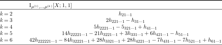
. See Table 1 for an example. The definition of the Kreweras number is given in § 7.
The
 $h$
-expansions of
 $\mathrm {I}_{\mu ^{(1)},\dots ,\mu ^{(k)}}[X;1,1]$
up to
 $k=6$
.

1.5 Organization
This paper is structured as follows. We commence with § 2, laying out the essential preliminary concepts and background information. In § 3, we review the plethystic formula for the Macdonald polynomials, studied by Garsia, Haiman, and Tesler [Reference Garsia, Haiman and TeslerGHT99]. By utilizing their formula, we proceed to establish Theorem 1.1(a) (the vanishing identity). Furthermore, we demonstrate Theorem 1.1(b), which proves shape independence and establishes a connection between Macdonald intersection polynomials and the characters of the diagonal coinvariant algebras. Sections 4, 5, and 6 are dedicated to proving Theorem 1.1(c). Section 4 provides some background on the shuffle formula
 $D_n[X;q,t]$
. Then we present a fermionic formula, which we call a lightning bolt formula (Theorem 4.6), due to Haglund, Haiman, Loehr, Remmel, and Ulyanov. Moving forward, in § 5, we explore generalized Macdonald polynomials for filled diagrams and the column exchange rule introduced in [Reference Kim, Lee and OhKLO22]. Section 6 proves the lightning bolt formula for Macdonald intersection polynomials, which is our key discovery that finalizes the proof of Theorem 1.1(c). In § 7, we investigate the specialization of Macdonald intersection polynomials at
 $q=t=1$
and present an
 $h$
-expansion formula (Theorem 1.3) that incorporates the Kreweras numbers. Section 8 presents a few remarks and discusses future questions. Finally, Appendix A includes a compilation of technical lemmas.
2. Preliminaries
2.1 Partitions
Let
 $n$
be a positive integer. A composition of
 $n$
is a sequence
 $\mu =(\mu _1,\dots ,\mu _\ell )$
of positive integers that sum to
 $n$
. We let
 $\ell (\mu )$
denote the length of
 $\mu$
, the number of its parts, and
 $|\mu |:=\sum _{i}\mu _i$
its size. We say that a composition
 $\mu$
is a partition if its parts are weakly decreasing. We use the notation
 $\mu \models n$
to indicate that
 $\mu$
is a composition of
 $n$
, and
 $\mu \vdash n$
to indicate that
 $\mu$
is a partition of
 $n$
. We use Young diagrams in French notation to display a partition as
 \begin{equation*} \mu =\{(i,j)\in \mathbb {Z}_+\times \mathbb {Z}_+ : j\le \mu _i\}, \end{equation*}
where each element of this set represents a cell in the diagram. The conjugate partition of
 $\mu$
, denoted by
 $\mu ^{\prime}=(\mu ^{\prime}_1,\mu ^{\prime}_2,\dots )$
, is obtained by reflecting the Young diagram of
 $\mu$
along the diagonal
 $y=x$
.
For a cell
 $u$
in a partition
 $\mu$
, we define the arm (coarm) of
 $u$
, denoted by
 $\mathrm {arm}_\mu (u)$
(
 $\mathrm {coarm}_\mu (u)$
), as the number of cells strictly to the right (left) of
 $u$
in the same row. Similarly, we define the leg (coleg) of
 $u$
, denoted by
 $\mathrm {leg}_\mu (u)$
(
 $\mathrm {coleg}_\mu (u)$
), as the number of cells strictly above (below)
 $u$
in the same column. For example, for a partition
 $\mu =(5,4,3,1)$
and a cell
 $u=(2,2)$
, we have
 $\mathrm {arm}_\mu (u)=2, \mathrm {coarm}_\mu (u)=1, \mathrm {leg}_\mu (u)=1$
and
 $\mathrm {coleg}(u)_\mu =1$
as displayed in the following diagram.

2.2 Symmetric functions
Let
 $\mathbf {Sym}$
be the graded ring of symmetric functions in infinite variables
 $X=x_1,x_2,\dots$
over the ground field
 $\mathbb {C}(q,t)$
. We use the notation from [Reference MacdonaldMac88] for families of symmetric functions indexed by a partition:
 $m_\lambda$
for the monomial symmetric function,
 $h_\lambda$
for the homogeneous symmetric function,
 $e_\lambda$
for the elementary symmetric function,
 $p_\lambda$
for the power sum symmetric function,
 $s_\lambda$
for the Schur function, and
 $J_\lambda$
for the integral form Macdonald polynomial (or Macdonald
 $J$
-polynomial). The (Hall) inner product on symmetric functions, denoted by
 $\langle -,-\rangle$
, is defined by
 \begin{equation*} \langle s_\lambda , s_\mu \rangle = \delta _{\lambda ,\mu }. \end{equation*}
The modified Macdonald polynomials are defined using a plethystic substitution as follows:
 \begin{equation*} \widetilde {H}_\mu [X;q,t] = t^{n(\mu )}J_\mu \bigg[\dfrac {X}{1-t^{-1}};q,t^{-1}\bigg], \end{equation*}
where
 $n(\mu )=\sum _i (i-1)\mu _i$
. Each of the above families of symmetric functions form a basis for
 $\mathbf {Sym}$
.
2.3 Quasisymmetric functions
Let
 $\mathbf {QSym}$
be the graded ring of quasisymmetric functions in infinite variables
 $X=x_1,x_2,\dots$
over the ground field
 $\mathbb {C}(q,t)$
. Given a composition
 $\alpha =(\alpha _1,\alpha _2,\dots ,\alpha _\ell )\models n$
, the monomial quasisymmetric function
 $M_\alpha [X]$
is defined by
 \begin{equation*} M_\alpha [X] := \sum _{i_1\lt i_2\lt \cdots \lt i_\ell } x_{i_1}^{\alpha _1}x_{i_2}^{\alpha _2}\cdots x_{i_\ell }^{\alpha _\ell }, \end{equation*}
and the (Gessel’s) fundamental quasisymmetric function [Reference GesselGes84]
 $F_\alpha [X]$
is defined by
 \begin{equation*} F_\alpha [X] := \sum _{\beta \le \alpha }M_\beta , \end{equation*}
where
 $\beta \le \alpha$
means we can obtain
 $\alpha$
by adding consecutive parts of
 $\beta$
. Each of the above two families forms a basis for
 $\mathbf {QSym}$
.
Compositions of
 $n$
are in one-to-one correspondence with the subsets of
 $[n-1]$
. We will define the natural bijection
 $\mathrm {Comp}$
from
 $2^{[n-1]}$
to compositions of
 $n$
by
 \begin{align*} \mathrm {Comp}:\{s_1\lt s_2\lt \cdots \lt s_\ell \} \mapsto (s_1,s_2-s_1,\dots ,s_\ell -s_{\ell -1},n-s_\ell ), \quad \mathrm {Comp}({\varnothing })=(n). \end{align*}
The inverse of
 $\mathrm {Comp}$
is denoted by
 $\mathrm {Set}$
. Under this correspondence, for a subset
 $S\subseteq [n-1]$
, we write
 $F_{n,S}$
as shorthand for
 $F_{\mathrm {Comp}(S)}$
. If
 $n$
is clear from the context, we write
 $F_{S}$
for
 $F_{n,S}$
. Given a permutation
 $w\in \mathfrak {S}_n$
, we will usually associate to it a fundamental quasisymmetric function
 $F_{\mathrm {iDes}(w)}$
, where
 \begin{equation*} \mathrm {iDes}(w):=\mathrm {Des}(w^{-1})=\left\{i:w^{-1}_i\gt w^{-1}_{i+1}\right\}. \end{equation*}
We end this section with a useful identity which will be used in § 6. For
 $n\ge 1$
, define a linear operator
 $E_n^\perp$
on
 $\mathbf {QSym}$
by
 \begin{align} E_{n}^\perp F_\alpha =\begin{cases} F_{\beta ^-} & \text {if} \ \alpha = (1^{(n-1)},\beta ),\\ 0 & \text {otherwise}, \end{cases} \end{align}
where
 $\beta ^-$
is the composition obtained by subtracting one from the first component of
 $\beta$
if
 $\beta _1\gt 1$
, with
 $\beta ^{-}=(\beta _2,\dots )$
otherwise. It is worth noting that for a composition
 $\beta =(b_1,\dots ,b_r)$
there are two compositions
 \begin{equation*} \alpha ^{(1)}=(\underbrace {1,\dots ,1}_{n-1},b_1+1,b_2,\dots ,b_r), \quad \alpha ^{(2)}=(\underbrace {1,\dots ,1}_{n},b_1,\dots ,b_r) \end{equation*}
such that
 $E_{n}^\perp F_{\alpha ^{(1)}}=E_{n}^\perp F_{\alpha ^{(2)}}=F_{\beta }$
. Then the skewing operator
 $e_n^\perp$
on symmetric functions is related to
 $E_n^\perp$
as follows.
Proposition 2.1 [Reference Gelfand, Krob, Lascoux, Leclerc, Retakh and ThibonGKLLRT95]. For a symmetric function
 $f$
, we have
 \begin{equation*} e_n^\perp f = E_n^\perp f, \end{equation*}
where
 $f$
on the right-hand side is considered a quasisymmetric function.
For the rest of the paper, we abuse the notation and refer to
 $E_n^{\perp }f$
as
 $e_n^{\perp }f$
for
 $f\in \mathbf {QSym}$
.
Remark 2.2. The ring
 $\mathbf {NSym}$
of noncommutative symmetric functions is the dual of the ring
 $\mathbf {QSym}$
of quasisymmetric functions with respect to the (extended) Hall inner product. The elementary noncommutative symmetric functions
 $E_\alpha$
form a basis for
 $\mathbf {NSym}$
. In addition, for a partition
 $\lambda$
,
 $E_\lambda$
descends to the elementary symmetric function
 $e_\lambda$
via natural surjection from
 $\mathbf {NSym}$
onto
 $\mathbf {Sym}$
. The operator
 $E_n^\perp$
is the adjoint operator of multiplying
 $E_n$
with respect to the Hall inner product. Although there is a choice of
 $E_n$
which descends to
 $e_n$
, regardless of choice Proposition 2.1 holds. For our purpose, we have chosen the elementary noncommutative symmetric functions
 $E_n$
.
3. Proof of Theorem 1.1 parts (a) and (b)
In this section, we prove two results concerning Macdonald intersection polynomials. The first is Theorem 1.1(a), the vanishing identity. The second is Theorem 1.1(b), which is an identity between the Macdonald intersection polynomials
 $\mathrm {I}_{\mu ^{(1)},\dots ,\mu ^{(k)}}[X;q,t]$
and
 $\nabla e_{k-1}$
. This, in particular, gives the shape independence, which asserts that
 \begin{equation*} \dfrac {1}{T_{\bigcap _{i=1}^k \mu ^{(i)}}}e_{n+1-k}^\perp \mathrm {I}_{\mu ^{(1)},\dots ,\mu ^{(k)}}[X;q,t] \end{equation*}
does not depend on partitions
 $\mu ^{(1)}, \dots , \mu ^{(k)}$
and
 $\mu$
.
3.1 Plethystic formula for the Macdonald polynomials
We first review the plethystic formula for Macdonald polynomials studied by Garsia, Haiman, and Tesler in [Reference Garsia and TeslerGT96, Reference Garsia, Haiman and TeslerGHT99]. To do so, we introduce some relevant notation and basic facts. Let
 $g[t_1,t_2,\dots ]$
be a Laurent series in the variables
 $t_1,t_2,\dots$
. If a symmetric function
 $f$
is expressed as the formal power series
 \begin{equation*} f = \hat {f}[p_1,p_2,\dots ], \end{equation*}
then the plethystic substitution of
 $g$
into
 $f$
is
 \begin{equation*} f[g] = \hat {f}[p_1,p_2,\dots ]|_{p_k\mapsto g[t_1^k,t_2^k,\dots ]}. \end{equation*}
We will use brackets to denote plethystic substitutions. We use two different minus signs,
 $-$
and
 $\epsilon$
, to mean
 \begin{equation*} p_k[-X]=-p_k[X] \quad \text { and } \quad p_k[\epsilon X] = (-1)^k p_k[X]. \end{equation*}
It is worth noting that for a symmetric function
 $f$
, we have
 \begin{equation*} \omega f [X] = f[-\epsilon X], \end{equation*}
where
 $\omega$
is the involution on
 $\mathbf {Sym}$
sending
 $p_\lambda \rightarrow (-1)^{|\lambda |-\ell (\lambda )}p_\lambda$
. We denote the biexponent generator for a given partition
 $\mu$
by
 $B_\mu (q,t)$
, which can be expressed as
 \begin{equation*}B_\mu (q,t) := \sum _{c\in \mu } q^{\mathrm {coarm}_\mu (c)}t^{\mathrm {coleg}_\mu (c)}.\end{equation*}
Additionally, we define
 $M := (1-q)(1-t)$
and
 $D_\mu =D_\mu (q,t) := MB_\mu (q,t) - 1$
.
Following the notation of [Reference Garsia and TeslerGT96], the
 $*$
-inner product, denoted by
 $\langle -, - \rangle _*$
, is defined by
 \begin{equation*}\langle p_{\rho },p_{\nu }\rangle _* = \begin{cases} (-1)^{|\rho |-\ell (\rho )} z_\rho \prod _i (1-q^{\rho _i})(1-t^{\rho _i}) & \text { if } \rho =\nu, \\ 0 & \text { otherwise,}\end{cases}\end{equation*}
where
 $z_\rho$
is the integer that makes
 $n!/z_\rho$
the number of permutations of cycle type
 $\rho$
. It is straightforward to check that
 $\langle f,g\rangle _*=\langle \omega (f),\omega (g)\rangle _*$
for any symmetric functions
 $f$
and
 $g$
. The modified Macdonald polynomials form an orthogonal basis with respect to the
 $*$
-inner product [Reference Garsia and TeslerGT96, Theorem 1.1]. In particular, we have
 \begin{equation} \big\langle \widetilde {H}_\mu ,\widetilde {H}_\lambda \big\rangle _*=\begin{cases} \tilde {h}_\mu (q,t)\tilde {h}^{\prime}_\mu (q,t) &\text { if } \mu = \lambda, \\ 0, &\text { otherwise,} \end{cases} \end{equation}
where
 \begin{equation*} \tilde {h}_\mu (q,t) =\prod _{c\in \mu }\big(q^{\mathrm {arm}_\mu (c)}-t^{\mathrm {leg}_\mu (c)+1}\big) \quad \text {and} \quad \tilde {h}^{\prime}_\mu (q,t)=\prod _{c\in \mu }(t^{\mathrm {leg}_\mu (c)}- q^{\mathrm {arm}_\mu (c)+1}). \end{equation*}
The
 $*$
-inner product has several useful properties, one of which is [Reference Garsia, Haiman and TeslerGHT99, Proposition 1.8]: for two symmetric functions
 $P$
and
 $Q$
of degree
 $n$
, we have
 \begin{equation} \langle P[X],Q[X] \rangle _* = \langle P[MX], \omega Q[X]\rangle , \end{equation}
where
 $\langle -,-\rangle$
is the usual Hall inner product.
Garsia, Haiman, and Tesler provided a general result for the
 $*$
-inner product with modified Macdonald polynomials, which extends the plethystic formula for the
 $(q,t)$
-Kostka polynomials due to Garsia and Tesler [Reference Garsia and TeslerGT96]. To state their result, it is helpful to introduce the notation
 $g^*[X] := g[X/M]$
for a symmetric function
 $g[X]$
. The main theorem of their work can be presented as follows.
Theorem 3.1 [Reference Garsia, Haiman and TeslerGHT99, Theorem 1.2]. For a symmetric function
 $f$
, define
 $\Pi ^{\prime}_f$
by
 \begin{equation*} \Pi ^{\prime}_f[X;q,t] := \nabla ^{-1} f[X-\epsilon ]. \end{equation*}
Then for every partition
 $\mu \vdash n \geq m$
we have
 \begin{equation*} \langle e^*_{n-m}f,\widetilde {H}_\mu \rangle _* = \Pi ^{\prime}_f[D_\mu ;q,t]. \end{equation*}
3.2 Proof of Theorem 1.1 parts (a) and (b)
Let
 $\mu$
be a partition of
 $n$
. By applying (3.2) and Theorem 3.1, we have
 \begin{align*} \Pi ^{\prime}_{f}[D_\mu ;q,t] &= \langle e_{n-m}f[MX], \omega \widetilde {H}_\mu \rangle =\langle f[MX], e_{n-m}^\perp \omega \widetilde {H}_\mu \rangle \\ &=\langle f[X], \omega (e_{n-m}^\perp \omega \widetilde {H}_\mu ) \rangle _*= \langle \omega f[X], e_{n-m}^\perp \omega \widetilde {H}_\mu \rangle _*. \end{align*}
For a partition
 $\lambda \vdash m$
, we let
 $f$
in the above equation be
 $\widetilde {H}_\lambda$
. We apply the well-known symmetry of modified Macdonald polynomials (e.g. Theorem 1.5 in [Reference Garsia and TeslerGT96]), which is
 \begin{equation*} \omega \widetilde {H}_\mu =T_\mu \mathrm {rev}(\widetilde {H}_\mu ), \end{equation*}
where
 $\mathrm {rev}$
is an involution on
 $\mathbf {Sym}$
defined by
 $(q,t)$
-reversal:
 \begin{equation*} \mathrm {rev}(f) = f|_{q\mapsto q^{-1}, t\mapsto t^{-1}}. \end{equation*}
Then we have
 \begin{align} \Pi ^{\prime}_{\widetilde {H}_\lambda }[D_\mu ;q,t] &= \langle \omega \widetilde {H}_\lambda [X], e_{n-m}^\perp \omega \widetilde {H}_\mu \rangle _* \nonumber\\&= \langle T_\lambda \mathrm{rev}(\widetilde {H}_\lambda ),T_\mu e^{\perp}_{n-m} \mathrm{rev}(\widetilde {H}_\mu )\rangle _{*} = T_\mu T_\lambda \langle \mathrm {rev}(\widetilde {H}_\lambda ), e^\perp _{n-m} \mathrm {rev}(\widetilde {H}_\mu )\rangle _*. \end{align}
To extract the operator
 $\mathrm {rev}$
to the outside of the
 $*$
-inner product, we need the following lemma.
Lemma 3.2. For two symmetric functions
 $f,g \in \mathbf {Sym}$
of degree
 $m$
, we have
 \begin{equation*} \langle \mathrm {rev}(f), \mathrm {rev}(g) \rangle _*= (qt)^m \mathrm {rev}\left (\langle f, g \rangle _* \right ). \end{equation*}
Proof. It suffices to show the claim for
 $p_{\rho }\mbox{ and }p_{\nu }$
for partitions
 $\rho ,\nu \vdash m$
. We have
 \begin{align*} \langle \mathrm {rev}(p_{\rho }), \mathrm {rev}(p_\nu ) \rangle _* &= \langle p_\rho , p_\nu \rangle _* = (-1)^{|\rho |-\ell (\rho )}z_\rho \delta _{\rho ,\nu } \prod _{i\ge 1}(1-q^{\rho _i})(1-t^{\rho _i}) \\ &= (qt)^m (-1)^{|\rho |-\ell (\rho )}z_\rho \delta _{\rho ,\nu } \prod _{i\ge 1}(1-q^{-\rho _i})(1-t^{-\rho _i}) = (qt)^m \mathrm {rev}\left (\langle p_\rho ,p_\nu \rangle _* \right ). \end{align*}
Applying Lemma 3.2 to (3.3) gives
 \begin{equation*} \dfrac {1}{(qt)^mT_\mu T_\lambda }\langle \widetilde {H}_\lambda , e_{n-m}^\perp \widetilde {H}_\mu \rangle _*= \mathrm {rev} (\Pi ^{\prime}_{\widetilde {H}_\lambda }[D_\mu ;q,t]). \end{equation*}
By using the orthogonality relation (3.1), we see that
 \begin{equation} e_{n-m}^\perp \widetilde {H}_\mu = (qt)^m T_\mu \sum _{\lambda \vdash m} \mathrm {rev} (\Pi ^{\prime}_{\widetilde {H}_\lambda }[D_\mu ;q,t] )\dfrac {T_\lambda \widetilde {H}_\lambda }{\tilde {h}_\lambda \tilde {h}^{\prime}_\lambda }. \end{equation}
Now, let
 $\mu \vdash n+1$
be a partition and let
 $\mu ^{(1)},\dots ,\mu ^{(k)}\subseteq \mu$
be
 $k$
distinct partitions such that
 \begin{equation*} |\mu \setminus \mu ^{(1)}|=\cdots =|\mu \setminus \mu ^{(k)}|=1. \end{equation*}
Then the Macdonald intersection polynomial can be written as
 \begin{equation*} \mathrm {I}_{\mu ^{(1)},\dots ,\mu ^{(k)}}[X;q,t] =\sum _{i=1}^k \prod _{j\neq i}\bigg(\frac {z_j}{z_j-z_i}\bigg) \widetilde {H}_{\mu ^{(i)}}, \end{equation*}
where we write
 $z_i=T_{\mu ^{(i)}}/T_\mu$
. Note that
 $T_{\mu ^{(i)}}=z_iT_\mu$
and
 $T_{\cap _{i=1}^k \mu ^{(i)}}=z_1\cdots z_k T_\mu$
. Then using (3.4) we can show that
 $e^\perp _{n-m}\mathrm {I}_{\mu ^{(1)},\dots ,\mu ^{(k)}}[X;q,t]$
is equal to
 \begin{align} &(qt)^m {z_1\cdots z_k T_\mu } \sum _{\lambda \vdash m} \bigg (\sum _{i=1}^k \frac {\mathrm {rev}(\Pi ^{\prime}_{\widetilde {H}_\lambda }[D_{\mu ^{(i)}};q,t] )}{\prod _{j\neq i}(z_j-z_i)} \bigg )\dfrac {T_\lambda \widetilde {H}_\lambda }{\tilde {h}_\lambda \tilde {h}^{\prime}_\lambda }\nonumber \\[5pt] &\quad =(qt)^m T_{\cap _{i=1}^k \mu ^{(i)}} \sum _{\lambda \vdash m} \bigg (\sum _{i=1}^k \frac {\mathrm {rev} (\Pi ^{\prime}_{\widetilde {H}_\lambda }[D_{\mu ^{(i)}};q,t] )}{\prod _{j\neq i}(z_j-z_i)} \bigg)\dfrac {T_\lambda \widetilde {H}_\lambda }{\tilde {h}_\lambda \tilde {h}^{\prime}_\lambda }. \end{align}
We will make use of a well-known equality, which we state as a lemma.
Lemma 3.3. Let
 $z_1,\ldots ,z_k$
be variables. Then for a polynomial
 $g(z)$
(in one variable
 $z$
) of degree less than
 $k-1$
, we have
 \begin{equation*}\sum _{i=1}^k \dfrac {g(z_i)}{\prod _{j \neq i} (z_j-z_i)}=0.\end{equation*}
If
 $g(z)$
is a polynomial of degree
 $k-1$
with leading term
 $az^{k-1}$
, then
 \begin{equation*}\sum _{i=1}^k \dfrac {g(z_i)}{\prod _{j \neq i} (z_j-z_i)}=(-1)^{k-1}a.\end{equation*}
Proof of Theorem
1.1(a) (Vanishing identity). Consider the expression in (3.5) and assume
 $m\lt k-1$
. Then the term
 \begin{align*} \mathrm {rev}(\Pi ^{\prime}_{\widetilde {H}_{\lambda}} [D_\mu ^{(i)};q,t]))&= \mathrm {rev}(\nabla ^{-1}\widetilde {H}_\lambda \left [D_\mu -\epsilon -Mz_i^{-1};q,t\right ]) \\[4pt] &=T_\lambda \widetilde {H}_\lambda \bigg[D_\mu (q^{-1},t^{-1}) -\epsilon - \dfrac {M}{qt}z_i;q^{-1},t^{-1}\bigg ] \end{align*}
is a polynomial in
 $z_i$
of degree
 $m$
which is less than
 $k-1$
. As a consequence, using Lemma 3.3, we have that (3.5) vanishes. This completes the proof.
Proof of Theorem
1.1(b). In (3.5), let
 $m=k-1$
. Then
 \begin{equation*} \mathrm {rev}(\Pi ^{\prime}_{\widetilde {H}_{\lambda}} \,[D_\mu ;q,t]))=T_\lambda \widetilde {H}_\lambda \bigg[D_\mu (q^{-1},t^{-1}) -\epsilon - \dfrac {M}{qt}z_i;q^{-1},t^{-1}\bigg] \end{equation*}
is a polynomial of degree
 $k-1$
in
 $z_i$
. Moreover, the leading term is equal to
 \begin{align*} T_\lambda \widetilde {H}_\lambda \bigg[-\dfrac {M}{qt};q^{-1},t^{-1}\bigg] &= \omega \widetilde {H}_\lambda \bigg[-\dfrac {M}{qt};q,t\bigg] \\[4pt]&=(-qt)^{1-k} \widetilde {H}_\lambda \left [M;q,t\right ] \\[4pt]&=(-qt)^{1-k} M \Pi _\lambda B_\lambda, \end{align*}
where
 $\Pi _{\lambda }$
is a constant associated to a partition
 $\lambda$
and is defined as
 \begin{equation*} \Pi _{\lambda }:=\prod _{c\in \lambda \setminus \{(1,1)\}}(1-q^{\mathrm {coarm}_{\lambda }(c)}t^{\mathrm {coleg}_{\lambda }(c)}). \end{equation*}
Here, the last equality can be obtained from the generalized Macdonald–Koornwinder reciprocity [Reference Garsia, Haiman and TeslerGHT99, Theorem 3.3] when
 $\mu =(1)$
. Using Lemma 3.3, (3.5) becomes
 \begin{align*} e_{n+1-k}^\perp \mathrm {I}_{\mu ^{(1)},\dots ,\mu ^{(k)}}[X;q,t] &= (qt)^{k-1}T_{\bigcap _{i=1}^k \mu ^{(i)}} \sum _{\lambda \vdash k-1} \bigg (\sum _{i=1}^k \prod _{j\neq i}\frac {1}{z_j-z_i} \mathrm {rev}(\Pi ^{\prime}_{\widetilde {H}_\lambda }[D_\mu ;q,t]))\bigg)\dfrac {T_\lambda \widetilde {H}_\lambda }{\tilde {h}_\lambda \tilde {h}^{\prime}_\lambda } \\&=T_{\bigcap _{i=1}^k \mu ^{(i)}} \sum _{\lambda \vdash k-1} \dfrac {M \Pi _\lambda B_\lambda T_\lambda \widetilde {H}_\lambda }{\tilde {h}_\lambda \tilde {h}^{\prime}_\lambda }=T_{\bigcap _{i=1}^k \mu ^{(i)}} \nabla e_{k-1}, \end{align*}
where the last equality is from [Reference HaimanHai02, Theorem 3.2].
4. The fermionic formula for the shuffle formula
4.1 Fermionic formulas
Several important families of
 $q$
-polynomials that arise in combinatorics and representation theory can be expressed using fermionic formulas. These formulas involve a sum of products of
 $q$
-multinomials and nonnegative powers of
 $q$
. The origin of these formulas can be traced back to the Bethe ansatz [Reference BetheBet93] and
 $q$
-Kostka polynomial
 $K_{\lambda ,\mu }(q)$
(see [Reference Kerov, Kirillov and ReshetikhinKKR86]). Similarly, we refer to a fermionic formula for the sums of products of
 $q$
-multinomials and nonnegative powers of
 $q$
and
 $t$
.
Garsia and Haiman [Reference Garsia and HaimanGH96a] introduced a rational function
 $C_n(q,t)$
called the
 $q,t$
-Catalan numbers and conjectured that
 $C_n(q,t)$
is the Hilbert series of the diagonal coinvariant alternants, or
 $\langle D_n[X;q,t], e_n\rangle$
. This number
 $C_n(q,t)$
specializes to the well-known
 $q$
-Catalan numbers
 \begin{equation*} q^{\binom {n}{2}}C_n(q,1/q) = C^{(1)}_n(q) \quad \text {and}\quad C_n(1,q)=C_n(q,1)=C^{(2)}_n(q), \end{equation*}
where
 $C^{(1)}_n(q)$
is the major-index generating function over Dyck words and
 $C^{(2)}_n(q)$
is the area generating function for Dyck paths, justifying the name
 $q,t$
-Catalan numbers. Haglund [Reference HaglundHag03] gave a fermionic formula for
 $C_n(q,t)$
:
 \begin{equation} C_n(q,t) = \sum _{\alpha \models n} t^{\sum _{i=1}^{\ell (\alpha )}(i-1)\alpha _i}q^{\sum _{i=1}^{\ell (\alpha )} \binom {\alpha _i}{2} } \prod _{1\le i\le \ell (\alpha )-1} \bigg(\begin{array}{c}\alpha _i + \alpha _{i+1} -1\\[3pt]\alpha _{i+1}\end{array}\bigg)_{\!\!q}. \end{equation}
Meanwhile, Haglund and Loehr [Reference Haglund and LoehrHL05] conjectured a fermionic formula for the Hilbert series of the diagonal coinvariant algebra, or
 $\mathcal {H}_n(q,t)=\langle D_n[X;q,t], e_{(1^n)} \rangle$
. This conjecture was eventually proved in [Reference Carlsson and MellitCM18, Reference Carlsson and OblomkovCO18], yielding the formula
 \begin{equation} \mathcal {H}_n(q,t) = \sum _{\sigma \in \mathfrak {S}_n}t^{\mathrm {maj}(\sigma )}\prod _{i=1}^{n} [u_i(\sigma )-1]_q, \end{equation}
where
 $\mathrm {maj}(\sigma )=\sum _{i\in \mathrm {Des}(\sigma )}i$
and
 $u_i$
is defined as follows. For a permutation
 $\sigma$
, define a sequence
 $\sigma ^{\prime}$
by setting
 $\sigma ^{\prime}_i=\sigma _i$
for
 $1\le i \le n$
and
 $\sigma ^{\prime}_{n+1}=0$
. For each
 $1 \le i \le n$
,
 $u_i(\sigma )$
is the length of the longest consecutive sequence
 $\sigma ^{\prime}_{i},\dots, \sigma ^{\prime}_{j}$
satisfying either of the following:
-
–
$\sigma ^{\prime}_{i},\dots, \sigma ^{\prime}_{j}$
has no descent; -
–
$\sigma ^{\prime}_{i},\dots, \sigma ^{\prime}_{j}$
has one descent and
$\sigma ^{\prime}_i\gt \sigma ^{\prime}_j$
.


In § 4.2, we review a generalization (Theorem 4.6) of these two fermionic formulas (4.1) and (4.2).
4.2 Modified labeled Dyck paths and the shuffle formula
The shuffle theorem concerns a combinatorial formula
 $D_n[X;q,t]$
for
 $\nabla e_n$
as a generating function over parking functions. Several equivalent formulations of
 $D_n[X;q,t]$
exist in the literature. For our purpose, we will use the version presented in [Reference Loehr and NieseLN14, Theorem 14] employing the concept of modified labeled Dyck paths, which Haglund and Loehr first investigated in [Reference Haglund and LoehrHL05].
Definition 4.1. A Dyck path of length
 $n$
is a lattice path from
 $(0,0)$
to
 $(n,n)$
that does not go below the line
 $y=x$
. We denote a Dyck path by a sequence of
 $E$
and
 $N$
, where
 $E$
is an eastward step and
 $N$
is a northward step. We say that a Dyck path has a corner at
 $(i,j)$
if there is an eastward step from
 $(i-1,j)$
to
 $(i,j)$
followed by a northward step from
 $(i,j)$
to
 $(i,j+1)$
. Given a Dyck path
 $\pi$
and a permutation
 $w$
, a labeled Dyck path
 $L(\pi ,w)$
is a Dyck path
 $\pi$
with its
 $i$
th eastward step and
 $i$
th northward step labeled by
 $w_{n+1-i}$
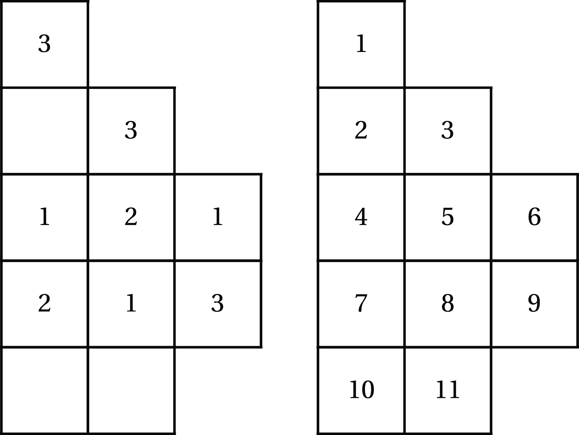
. For example, in the left diagram of Figure 1,
 $\pi =NNNENNENEEEE$
and
 $w=326514$
, so we have
 \begin{equation*} L(\pi ,w)=((N,4),(N,1),(N,5),(E,4),(N,6),(N,2),(E,1),(N,3),(E,5),(E,6),(E,2),(E,3)). \end{equation*}
The permutation
 $w$
can be obtained from
 $L(\pi ,w)$
by reading labels of the northward steps from top to bottom (or, equivalently, by reading labels of the eastward steps from right to left). We say that a pair
 $(\pi ,w)$
is a modified labeled Dyck path if for each corner of
 $\pi$
at
 $(i,j)$
, the label of the
 $i$
th eastward step is less than the label of the
 $(j+1)$
th northward step in
 $L(\pi ,w)$
. We represent a modified labeled Dyck path
 $(\pi ,w)$
by a Dyck path
 $\pi$
and a permutation
 $w$
assigned to the diagonal
 $y=x$
from top to bottom.
The set of modified labeled Dyck paths of length
 $n$
will be denoted by
 $\mathrm {MLD}(n)$
. We call a cell an
 $(i, j)$
-box if
 $i$
and
 $j$
are the
 $x$
- and
 $y$
-coordinates of its upper-right corner. Then for a pair
 $(\pi ,w)$
of a Dyck path
 $\pi$
of length
 $n$
and a permutation
 $w$
of length
 $n$
, the quantity
 $\mathrm {area}^{\prime}(\pi ,w)$
is defined as the number of pairs
 $(i,j)$
such that the
 $(i,j)$
-box lies between
 $\pi$
and the diagonal
 $y=x$
and the label of the
 $i$
th eastward step is less than the label of the
 $j$
th northward step in
 $L(\pi ,w)$
.
Given a Dyck path
 $\pi$
of length
 $n$
, we define its bounce path as follows. Begin at
 $(0,0)$
and move northward until the beginning of an eastward step is encountered. Then, travel eastward until the diagonal
 $y=x$
is reached. From this point, repeat the process by traveling northward until the next eastward step is encountered and then moving eastward until the diagonal
 $y=x$
is reached. Continue this manner until we reach
 $(n,n)$
. The bounce vector
 $\overrightarrow {b}(\pi )=(\alpha _1,\alpha _2,\dots )$
associated to the Dyck path is a composition of
 $n$
, obtained by reading the lengths of the individual bounces of the path from bottom to top. Then we define
 $\mathrm {bounce}(\pi )$
to be
 $\sum _{i=1}^{\ell (\alpha )}(i-1)\alpha _i$
.
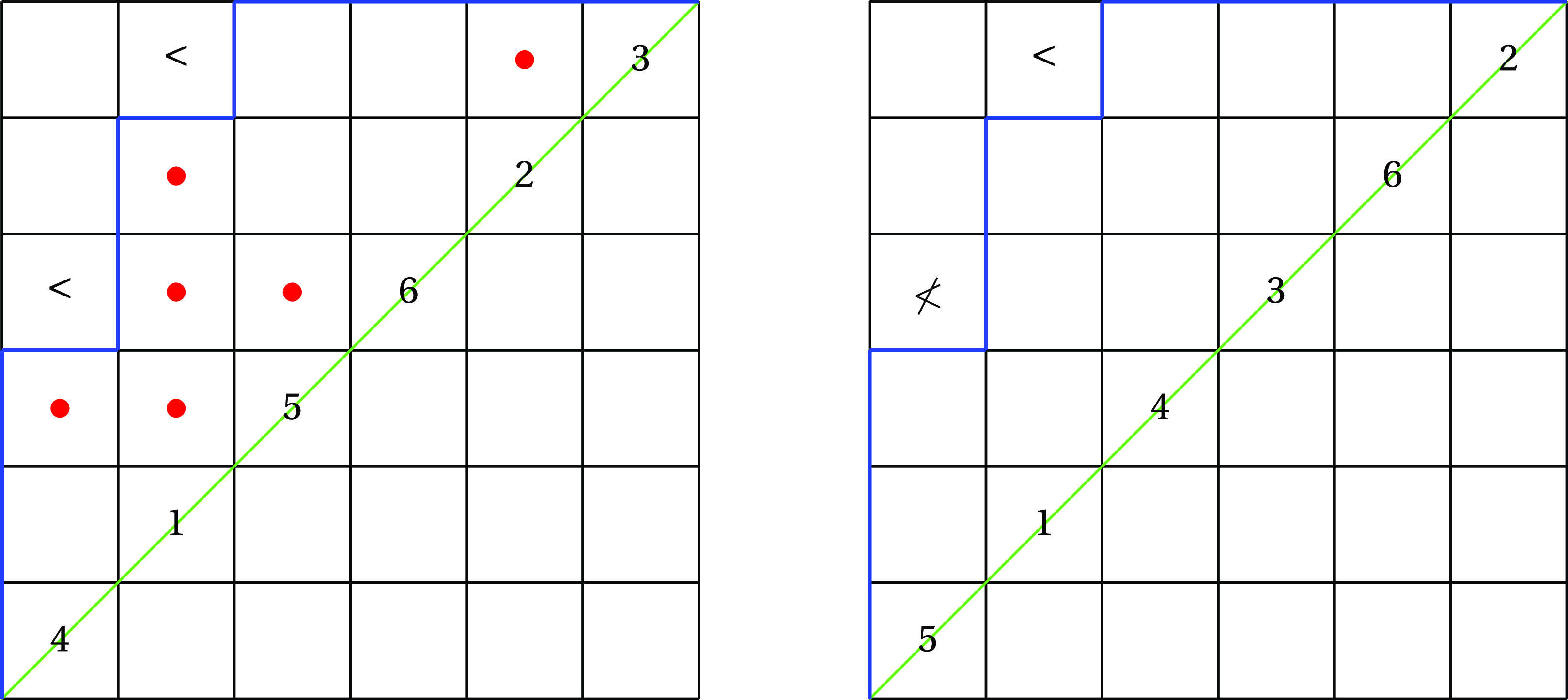
Example 4.2. On the left in Figure 1, a modified labeled Dyck path is depicted. On the other hand, the labeled Dyck path on the right in Figure 1 is not a modified labeled Dyck path because the label of the eastward step at the first corner is 5, which is greater than the label of the northward step, 3.
Let
 $(\pi ,w)$
be the modified labeled Dyck path shown on the left in Figure 1. The bounce vector associated with
 $\pi$
is
 $\overrightarrow {b}(\pi )=(3,3)$
, and
 $\mathrm {bounce}(\pi )=3$
. Additionally, six boxes (indicated with dots on the left in Figure 1) are located between the Dyck path and the main diagonal, where the label below the box is smaller than the label to its right. Therefore, we have
 $\mathrm {area}^{\prime}(\pi ,w)=6$
.
An example and a nonexample of a modified labeled Dyck path.

The following theorem reformulates the shuffle formula
 $D_n[X;q,t]$
in terms of modified labeled Dyck paths.
Theorem 4.3 [Reference Loehr and NieseLN14, Theorem 14]. We have
 \begin{equation*} D_n[X;q,t]=\sum _{(\pi ,w)\in \mathrm {MLD}(n)}t^{\mathrm {bounce}(\pi )}q^{\mathrm {area}^{\prime}(\pi ,w)}F_{\mathrm {iDes}(w)}. \end{equation*}
In other words, the shuffle theorem is equivalent to the identity
 \begin{equation*} \nabla e_n=\sum _{(\pi ,w)\in \mathrm {MLD}(n)}t^{\mathrm {bounce}(\pi )}q^{\mathrm {area}^{\prime}(\pi ,w)}F_{\mathrm {iDes}(w)}. \end{equation*}
4.3 The fermionic formula
For a (quasi)symmetric function
 $f$
of degree
 $n$
and a composition
 $\beta \models n$
, we denote by
 $[F_{\beta }](f)$
the coefficient of
 $F_{\beta }$
in the expansion of
 $f$
into fundamental quasisymmetric functions. Then the following lemma is immediate.
Lemma 4.4. For a composition
 $\beta =(\beta _1,\beta _2,\dots )$
of
 $n$
, let
 $e_\beta =e_{\beta _1}e_{\beta _2}\cdots$
be the elementary symmetric function. Then for a symmetric function
 $f$
of homogeneous degree
 $n$
, we have
 \begin{equation*} \langle f, e_{\beta }\rangle = \sum _{\substack {\alpha \models n \\ [n-1]\setminus \mathrm {Set}(\beta ) \subseteq \mathrm {Set}(\alpha ) }}[F_\alpha ](f), \end{equation*}
where the map
 $\mathrm {Set}$
is the bijection between compositions of
 $n$
and
 $2^{[n-1]}$
.
Proof. This follows from applying Proposition 2.1.
It is easy to check that given a permutation
 $w\in \mathfrak {S}_n$
, we have
 \begin{equation} \langle F_{\mathrm {Des}(w)}),e_{\beta }\rangle =1 \quad \text {if and only if}\quad \{i: w_{i}\lt w_{i+1}\}\subseteq \mathrm {Set}(\beta ). \end{equation}
Note that (4.1) and (4.2) give fermionic formulas for
 $\langle D_n[X;q,t],e_{n}\rangle$
and
 $\langle D_n[X;q,t],e_{(1^n)}\rangle$
, respectively. We will present a fermionic formula for
 $\langle D_{n}[X;q,t],e_{\beta }\rangle$
for general compositions
 $\beta \models n$
, which essentially follows from [Reference Haglund, Haiman, Loehr, Remmel and UlyanovHHLRU05, Equation (63)]. With that purpose in mind, we introduce some notation.
For positive integers
 $i\mbox{ and }j$
, the lightning bolt set
 $\mathrm {LB}(i,j)$
is the set of positions that are weakly above
 $(i,j-1)$
together with the positions that are weakly below
 $(i,j)$
:
 \begin{equation*} \mathrm {LB}(i,j) := \{(a,j-1):a\le i\} \cup \{(a,j):a\ge i\}. \end{equation*}
Here, we have used matrix coordinates for
 $(i, j)$
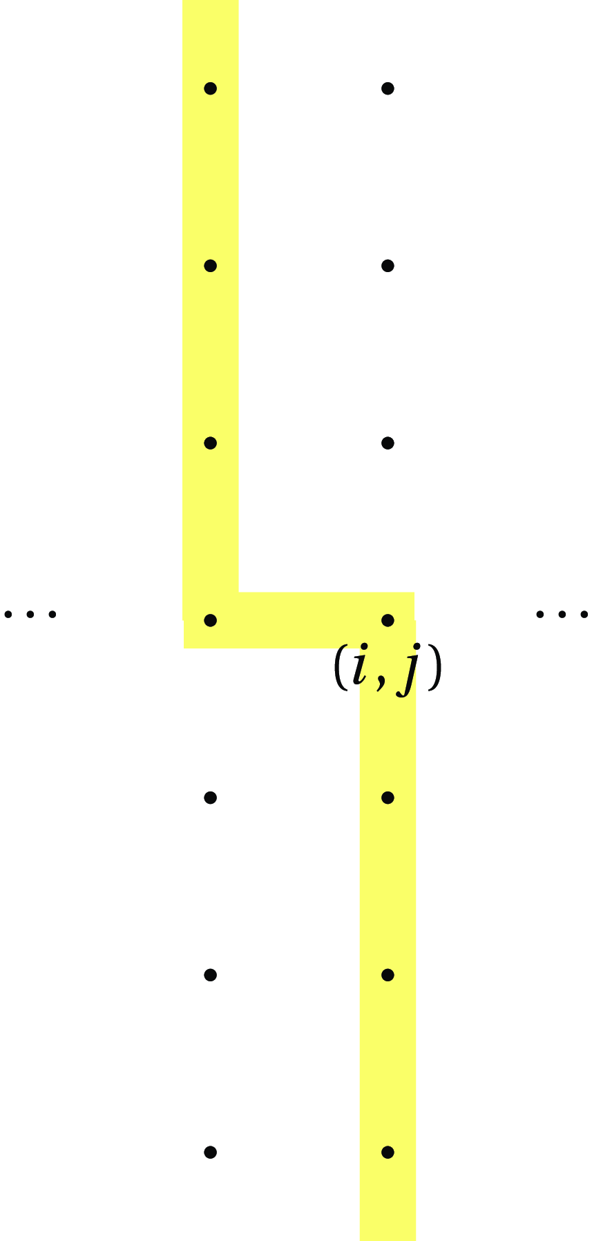
. Illustratively, the set
 $\mathrm {LB}(i,j)$
can be represented as in Figure 2.
The lightning bolt set
 $\mathrm {LB}(i,j)$
.

We denote the set of nonnegative integer matrices by
 $\mathrm {Mat}^{\ge 0}=\bigcup _{1\le r,\ell }{\mathrm {Mat}^{\ge 0}_{r\times \ell }}$
, where
 $\mathrm {Mat}^{\ge 0}_{r\times \ell }$
is the set of nonnegative integer matrices with
 $r$
rows and
 $\ell$
columns. A row sum vector (respectively, column sum vector) of a matrix
 $M$
is denoted by
 $\mathrm {rsum}(M)$
(respectively,
 $\mathrm {csum}(M)$
), and let
 $|M|$
be the sum of entries of
 $M$
. For example, the matrix
 \begin{equation*} M=\bigg[\begin{matrix} a & \quad b \\ c & \quad d \end{matrix}\bigg] \end{equation*}
gives
 $\mathrm {rsum}(M)=(a+b,c+d)$
,
 $\mathrm {csum}(M)=(a+c,b+d)$
, and
 $|M|= a+b+c+d$
. For a matrix
 $M\in \mathrm {Mat}^{\ge 0}_{r\times \ell }$
and
 $1\le i \le r, 2 \le j \le \ell$
, we define
 $\mathrm {lb}(M;(i,j))$
as
 \begin{equation*} \mathrm {lb}(M;(i,j)) := \sum _{(a,b)\in \mathrm {LB}(i,j)}M_{a,b}. \end{equation*}
We also define
 $\mathrm {lb}(M)$
as
 \begin{equation*} \mathrm {lb}(M) := \binom {M_{1,1}+\dots +M_{r,1}}{M_{1,1},\dots ,M_{r,1}}_{\!\!q} \prod _{\substack {1\le i \le r\\ 2\le j \le \ell }} \binom {\mathrm {lb}(M;(i,j))-1}{M_{i,j}}_q, \end{equation*}
where the first term on the right is the
 $q$
-multinomial coefficient and the second term is the product of
 $q$
-binomial coefficients. We use the convention
 $\binom {-1}{0}_q=\binom {0}{0}_q=1$
. The following basic property of
 $\mathrm {lb}(M)$
is worth noting.
Lemma 4.5. For a matrix
 $M$
such that
 $\mathrm {lb}(M)\neq 0$
, there exists a composition
 $\alpha$
such that
 $\mathrm {csum}(M)=(\alpha ,0,\dots ,0)$
. For such an
 $M$
, let
 $M^{\prime}$
be the matrix obtained from
 $M$
by restricting to the first
 $\ell (\alpha )$
columns. Then we have
 $\mathrm {lb}(M)=\mathrm {lb}(M^{\prime})$
.
Proof. Assume there exists
 $j$
such that the
 $j$
th column of
 $M$
is a zero column while the
 $(j+1)$
th column is not a zero column. Let
 $i$
be the maximal integer such that
 $M_{i,j+1}\neq 0$
. Then we have
 $\mathrm {lb}(M;(i,j+1))=M_{i,j+1}$
and thus
 $\binom {M_{i,j+1}-1}{M_{i,j+1}}_q=0$
. We conclude that
 $\mathrm {lb}(M)=0$
. Therefore, to have
 $\mathrm {lb}(M)\neq 0$
, zero columns of
 $M$
must be on the right of nonzero columns of
 $M$
, implying
 $\mathrm {csum}(M)=(\alpha ,0,\dots ,0)$
for some composition
 $\alpha$
.
Note that
 $M$
can be obtained from
 $M^{\prime}$
by appending zero columns to the right. It is easy to check that appending a zero column to the right does not change the value
 $\mathrm {lb}(-)$
.
We now state the fermionic formula for
 $\langle D_n[X;q,t],e_{\beta }\rangle$
of Haglund et al. [Reference Haglund, Haiman, Loehr, Remmel and UlyanovHHLRU05]. Their original formulation uses the concept of a ‘
 $\beta$
-shuffle’, whereas we employ a different formulation. Specifically,
 $\langle D_n[X;q,t],e_{\beta }\rangle$
is expressed as a sum of products of
 $\mathrm {lb}(M)$
and nonnegative powers of
 $q$
and
 $t$
over all nonnegative integer matrices
 $M$
of size
 $\ell (\beta ) \times \ell (\alpha )$
that satisfy certain constraints.
Theorem 4.6 [Reference Haglund, Haiman, Loehr, Remmel and UlyanovHHLRU05]. For a composition
 $\beta \models n$
, we have
 \begin{equation*} \langle D_n[X;q,t],e_{\beta }\rangle = \sum _{\alpha \models n} t^{\sum _{i=1}^{\ell (\alpha )}(i-1)\alpha _i} \sum _{\substack {M \in \mathrm {Mat}^{\ge 0} \\ \mathrm {rsum}(M)=\beta \\ \mathrm {csum}(M)=\alpha }} q^{\sum _{i,j}\binom {M_{i,j}}{2} } \mathrm {lb}(M). \end{equation*}
For the sake of completeness, we provide a proof in § 4.4 of our formulation. We end this section with an explanation of how (4.1) and (4.2) can be regarded as special cases of the theorem above. Observe that the fermionic formula for
 $q,t$
-Catalan numbers (4.1) can be derived directly from Theorem 4.6 by setting
 $\beta =(n)$
.
To demonstrate that (4.2) also follows from Theorem 4.6, let
 $\beta =(1^n)$
. In this scenario, the summation is conducted over all nonnegative integer matrices with
 $n$
rows, each of whose rows contains precisely one nonzero entry, which is 1.
We can establish a correspondence between such matrices
 $M$
and permutations
 $\sigma (M)$
as follows: read the row numbers of the ones from top to bottom, starting from the rightmost column and moving leftward. For instance, the matrix
 \begin{equation} M=\begin{bmatrix} 1 & \quad 0 & \quad 0\\ 0 & \quad 1 & \quad 0\\ 1 & \quad 0 & \quad 0\\ 0 & \quad 0 & \quad 1 \end{bmatrix} \end{equation}
corresponds to the permutation
 $\sigma (M)=4213$
. For a permutation
 $\sigma \in \mathfrak {S}_n$
, let
 $\mathrm {Des}(\sigma )=\{d_1\lt \cdots \lt d_{\ell }\}$
. Then for
 $1\leq i \leq \ell +1$
, we define a word
 $\sigma ^{(i)}:=\sigma _{d_{i-1}+1}\cdots \sigma _{d_{i}}$
where we set
 $d_0=0$
and
 $d_{\ell +1}=n$
. In other words,
 $\sigma ^{(i)}$
is the
 $i$
th increasing run of
 $\sigma$
. For example, for
 $\sigma =4213$
we have
 $\sigma ^{(1)}=4$
,
 $\sigma ^{(2)}=2$
, and
 $\sigma ^{(3)}=13$
. Now we define an
 $n\times (\ell +1)$
matrix
 $M(\sigma )$
by letting its entries be defined as follows:
 \begin{equation*} M(\sigma )_{i,j}:= \begin{cases} 1&\text { if } i\text { appears in } \sigma ^{(\ell +2-j)},\\ 0&\text { otherwise}. \end{cases} \end{equation*}
It is straightforward to see that
 $M(4213)$
is the matrix
 $M$
given in (4.4). We claim that
 $M(\sigma )$
is the unique matrix
 $M$
with
 $\mathrm {lb}(M)\neq 0$
among matrices satisfying
 $\sigma (M)=\sigma$
. To see this, suppose that
 $M^{\prime}$
is a matrix with
 $\sigma (M^{\prime})=\sigma$
and
 $M^{\prime}\neq M(\sigma )$
. Then there exists
 $\sigma ^{(r)}$
such that there are distinct
 $i, i^{\prime} \in \sigma ^{(r)}$
and distinct
 $j, j^{\prime}$
where
 $M_{i,j} = 1$
and
 $M_{i^{\prime},j^{\prime}} = 1$
. Assume that
 $\sigma ^{(i)}$
starts in the
 $b$
th column and let
 $a$
be the maximal integer such that
 $M^{\prime}_{a,b}=1$
. Then we have
 $M^{\prime}_{c,d}=0$
for all
 $(c,d)\in \mathrm {LB}(a,b)\setminus \{(a,b)\}$
. This implies
 $\binom {\mathrm {lb}(M^{\prime};(a,b))-1}{M^{\prime}_{a,b}}=\binom {0}{1}_q=0$
and hence
 $\mathrm {lb}(M^{\prime})=0$
. For example,
 \begin{equation*} M^{\prime}=\begin{bmatrix} 0& \quad 1 & \quad 0 & \quad 0\\ 0& \quad 0 & \quad 1 & \quad 0\\ 1& \quad 0 & \quad 0 & \quad 0\\ 0& \quad 0 & \quad 0 & \quad 1 \end{bmatrix} \end{equation*}
yields
 $\sigma (M^{\prime})=4213$
and
 $\sigma ^{(3)}=13$
lies in the first and the second columns. We have
 $\mathrm {lb}(M^{\prime})=0$
since
 $\binom {\mathrm {lb}(M^{\prime};(1,2))-1}{M^{\prime}_{1,2}}=\binom {0}{1}_q = 0$
.
Let
 $\sigma$
be a permutation with
 $\mathrm {Des}(\sigma ) = \{d_1\lt \cdots \lt d_\ell \}$
, and consider
 $M=M(\sigma )$
. For
 $j\gt 1$
pick any
 $i$
such that
 $M_{i,j}=1$
and let
 $m$
be the corresponding position in
 $\sigma (M)=\sigma$
, i.e.
 $\sigma _m = i$
. Then it is easy to check that
 $u_m(\sigma )=\mathrm {lb}(M;(i,j))$
. Entries equal to 1 in the first column of
 $M$
correspond to
 $\sigma ^{(\ell +1)}=\sigma _{d_{\ell }+1}\cdots \sigma _{n}$
, and for each
 $d_{\ell }+1\leq m\leq n$
we have
 $u_m(\sigma )=n+2-m$
. Therefore we have
 \begin{equation*} \prod _{m=d_{\ell }+1}^{n}[u_m(\sigma )-1]_q=[n-d_{\ell }]_q\cdots [1]_q = [n-d_\ell ]_q!\,, \end{equation*}
which equals
 $\binom {M_{1,1}+\dots +M_{n,1}}{M_{1,1},\dots ,M_{n,1}}_q=\binom {n-d_\ell }{1,\dots ,1}_q$
. This shows that
 $\mathrm {lb}(M(\sigma ))=\prod _{m=1}^{n}[u_m(\sigma )-1]_q$
. Since we have
 $\mathrm {maj}(\sigma )=\sum _{i\ge 1} (i-1)\alpha _i$
where
 $\alpha =\mathrm {csum}(M(\sigma ))$
, letting
 $\beta =(1^n)$
in Theorem 4.6 gives (4.2).
4.4 Proof of Theorem 4.6
In this subsection, we consider only
 $M\in \mathrm {Mat}^{\geq 0}$
without a zero column or a zero row. We provide a combinatorial interpretation of
 $\mathrm {lb}(M)$
in terms of modified labeled Dyck paths (Proposition 4.8). To that end, we fix a matrix
 $M \in \mathrm {Mat}^{\ge 0}_{r\times \ell }$
. We define a vector
 $m\in \mathbb {Z}_{\ge 0}^{r\ell }$
obtained by reading the entries of
 $M$
from left to right and top to bottom, i.e.
 $m_{n(i,j)}= M_{i,j}$
, where
 $n(i,j):= \ell (i-1)+j$
for
 $1 \leq j \leq \ell$
. Then we set
 \begin{equation*} I(M;(i,j)) := \bigg[1 + \sum _{a=1}^{n(i,j)-1} m_a, \sum _{a=1}^{n(i,j)} m_a\bigg]. \end{equation*}
Now we define
 $\mathrm {MLD}(M)$
to be the set of all modified labeled Dyck paths
 $(\pi ,w)$
that satisfy the following conditions:
-
(1) the bounce vector
$\overrightarrow {b}(\pi )=(\alpha _1,\alpha _2,\dots )=\mathrm {csum}(M)$
; -
(2) the set of entries of
$w$
on the bounce corresponding to column
$(\ell -j+1)$
is equal to
$\bigcup\nolimits _{i=1}^{r} I(M;(i,j))$
; -
(3) elements of
$I(M;(i,j))$
are decreasing in
$w$
.


Example 4.7. Let
 $M=\left (\left[\begin{smallmatrix} 1 & \quad\!\!\!\! 2\\ 2 & \quad\!\!\!\!1 \end{smallmatrix}\right] \right )$
. Then the associated vector
 $m = (1,2,2,1)$
and intervals
 $I(M;(i,j))$
are
 \begin{equation*} I(M;(1,1))=\{1\}, \quad I(M;(1,2))=\{2,3\}, \quad I(M;(2,1))=\{4,5\}, \quad I(M;(2,2))=\{6\}. \end{equation*}
By definition, a modified labeled Dyck path
 $(\pi ,w)\in \mathrm {MLD}(M)$
satisfies the following conditions:
-
(1) the bounce vector
$\overrightarrow {b}(\pi )=(3,3)$
; -
(2)
$I(M;(1,1))\cup I(M;(2,1))=\{1,4,5\}=\{w_4,w_5,w_6\},\quad \text{and}\quad I(M;(1,2))\cup I(M;(2,2))=\{2,3,6\}= \{w_1,w_2,w_3\}$
; -
(3) 4 and 5 are placed in decreasing order and 2 and 3 are placed in decreasing order in
$w$
.


The modified labeled Dyck path on the left in Figure 1 belongs to
 $\mathrm {MLD}(M)$
. For the same Dyck path
 $\pi$
and
 $w=632541$
, one can check that
 $(\pi ,w)\in \mathrm {MLD}(M)$
.
For
 $(\pi ,w)\in \mathrm {MLD}(M)$
, we have
 $\langle F_{\mathrm {iDes}(w)},e_{\beta }\rangle =1$
if
 $\beta =\mathrm {rsum}(M)$
. Conversely, given
 $(\pi ,w)\in \mathrm {MLD}(n)$
such that
 $\langle F_{\mathrm {iDes}(w)},e_{\beta }\rangle =1$
for some
 $\beta \models n$
, we define a matrix
 $M$
as follows. Let
 $\alpha =\overrightarrow {b}(\pi )$
be the bounce vector. We also let
 $s_j=\sum _{j\lt b} \alpha _b$
and
 $t_i=\sum _{b\lt i} \beta _b$
. Then we define the
 $\ell (\beta ) \times \ell (\alpha )$
matrix
 $M$
by letting its entries be as follows:
 \begin{align*} M_{i,j}=\left |\left \{w_{s_j+1}, \dots , w_{s_{j-1}}\right \}\ \cap \left [t_{i}+1,t_{i+1}\right ]\right |. \\[-12pt] \end{align*}
Note that we have
 $(\pi ,w)\in \mathrm {MLD}(M)$
and
 $\mathrm {rsum}(M)=\beta$
. Furthermore,
 $M$
is the unique matrix with this property. Therefore, together with Theorem 4.3, we obtain
 \begin{align} \langle D_{n}[X;q,t],e_{\beta }\rangle =1= \sum _{\substack {M\in \mathrm {Mat}^{\ge 0} \\ \mathrm {rsum}(M)=\beta }}\sum _{{(\pi ,w)\in \mathrm {MLD}(M)}}t^{\mathrm {bounce}(\pi )}q^{\mathrm {area}^{\prime}(\pi ,w)}. \end{align}
Proposition 4.8. Let
 $M\in \mathrm {Mat}^{\ge 0}_{r\times \ell }$
. Then
 $\mathrm {lb}(M)$
is a generating function for
 $\mathrm {area}^{\prime}$
over all modified labeled Dyck paths
 $\mathrm {MLD}(M)$
:
 \begin{equation*} \mathrm {lb}(M) = q^{-\sum _{i,j}\binom {M_{i,j}}{2}}\sum _{(\pi ,w)\in \mathrm {MLD}(M)} q^{\mathrm {area}^{\prime}(\pi ,w)}. \end{equation*}
Proof. Let
 $\ell = 1$
. If
 $(\pi , w) \in \mathrm {MLD}(M)$
then the bounce vector of
 $\pi$
is of length 1, so
 $\pi$
must be the full Dyck path, i.e.
 $\pi = N \cdots N E \cdots E$
. For a permutation
 $w \in \mathfrak {S}_{|M|}$
,
 $(\pi , w) \in \mathrm {MLD}(M)$
if and only if the elements in
 $I(M; (i, 1))$
are in decreasing order in
 $w$
for all
 $i$
. Then there is a natural bijection
 \begin{equation*} \phi : \mathrm {MLD}(M) \rightarrow W_{M_{1,1}, M_{2,1}, \dots , M_{r,1}}, \end{equation*}
where
 $W_{M_{1,1}, M_{2,1}, \dots , M_{r,1}}$
is the set of words of consisting of
 $M_{i,1}$
instances of
 $i$
, and
 $\phi (\pi ,w)$
is defined as the word obtained from the permutation
 $w$
by replacing entries in the interval
 $I(M; (i, 1))$
with
 $i$
. Then, note that
 \begin{equation} \mathrm {area}^{\prime}(\pi , w) = \mathrm {inv}(w) = \sum _{i=1}^r \binom {M_{i,1}}{2} + \mathrm {inv}(\phi (\pi ,w)). \end{equation}
One can see this by dividing the contributions to
 $\mathrm {inv}(w)$
into two cases. The first case consists of the pair of entries in the same interval
 $I(M; (i, 1))$
for some
 $i$
, contributing
 $\sum _{i=1}^r \binom {M_{i,1}}{2}$
. The second case consists of the pair of integers in different intervals,
 $I(M; (i, 1))$
and
 $I(M; (i^{\prime}, 1))$
, which are out of order. The contribution of the latter case is given by the usual inversions of
 $\phi (\pi ,w)$
. By (4.6), we have
 \begin{equation*} \sum _{(\pi , w) \in \mathrm {MLD}(M)} q^{\mathrm {area}^{\prime}(\pi , w)} = q^{\sum _{i=1}^r \binom {M_{i,1}}{2}} \binom {M_{1,1} + \dots + M_{r,1}}{M_{1,1}, \dots , M_{r,1}}_{\!q} = q^{\sum _{i=1}^r \binom {M_{i,1}}{2}} \mathrm {lb}(M). \end{equation*}
Here, we have used the fact that the inversion generating function of
 $W_{M_{1,1}, M_{2,1}, \dots , M_{r,1}}$
is the
 $q$
-multinomial coefficient
 $\binom {M_{1,1} + \dots + M_{r,1}}{M_{1,1}, \dots , M_{r,1}}_{\!q}$
.
Suppose that
 $\ell \gt 1$
, and let us proceed by induction on the sum
 $n=|M|$
. We are dealing with
 $M$
without a zero column, so the base case
 $|M|=1$
has been covered. Let
 $c$
be the smallest index
 $i$
such that
 $M_{i,\ell }\neq 0$
, and let
 $M^{\prime}$
be the matrix obtained from
 $M$
by replacing
 $M_{c,\ell }$
with zero. If the rightmost column of
 $M^{\prime}$
is a zero column, we simply erase that column.
Let
 $s=\mathrm {lb}(M;(c,\ell ))$
and let
 $W^{0}_{s,M_{c,\ell }}$
be the set of 0-1 sequences of length
 $s$
with
 $M_{c,\ell }$
ones starting with a zero. Suppose we construct a bijection
 \begin{align*} \Phi :\mathrm {MLD}(M) &\rightarrow \mathrm {MLD}(M^{\prime})\times W^{0}_{s,M_{c,\ell }}\\ (\pi ,w) &\mapsto (\Phi _1(\pi ,w), \Phi _2(\pi ,w)) \end{align*}
such that
 \begin{equation} \mathrm {area}^{\prime}(\pi ,w)=\mathrm {area}^{\prime}\left (\Phi _1(\pi ,w)\right ) + \mathrm {inv}\left (\Phi _2(\pi ,w)\right ) + \binom {M_{c,\ell }}{2}. \end{equation}
Then we have
 \begin{align*} \sum _{(\pi ,w)\in \mathrm {MLD}(M)} q^{\mathrm {area}^{\prime}(\pi ,w)} & = q^{\binom {M_{c,\ell }}{2}} \sum _{(\pi ,w)\in \mathrm {MLD}(M^{\prime})} q^{\mathrm {area}^{\prime}(\pi ,w)} \sum _{\sigma \in W^{0}_{s,M_{c,\ell }}}q^{\mathrm {inv}(\sigma )}\\ &=q^{\sum _{i,j}\binom {M_{i,j}}{2}}\mathrm {lb}(M^{\prime}) \binom {\mathrm {lb}(M;(c,\ell ))-1}{M_{c,\ell }}_{\!q}\\ &=q^{\sum _{i,j}\binom {M_{i,j}}{2}}\mathrm {lb}(M). \\[-12pt] \nonumber \end{align*}
Here, the first equality follows from (4.7). The second equality follows from the induction hypothesis, and the last equality follows from the definition of
 $\mathrm {lb}(M)$
. Therefore, it suffices to construct such a bijection
 $\Phi$
satisfying (4.7).
Given a modified labeled Dyck path
 $(\pi ,w)\in \mathrm {MLD}(M)$
, recall that each step in
 $\pi$
has an associated label which we encoded in
 $L(\pi ,w)$
(see Definition 4.1). Let
 $\mathrm {csum}(M)=\alpha$
then
 $\pi$
must pass through specific points
 $X_0$
and
 $X_1$
given by
 \begin{align} X_{0} = \bigg(\sum _{1\le j \le \ell -2}\alpha _j,\sum _{1\le j \le \ell -1}\alpha _j\bigg) \quad \text {and} \quad X_{1} = \bigg(\sum _{1\le j \le \ell -1}\alpha _j,n\bigg). \\[-14pt] \nonumber \end{align}
In other words, the subpath from
 $X_0$
to
 $X_1$
corresponds to the last bounce of
 $\pi$
and we let
 $P(\pi ,w)$
be a subsequence of
 $L(\pi ,w)$
for this subpath, denoted by
 $P(\pi ,w)=(P_1,\dots ,P_{\alpha _{\ell -1}+\alpha _{\ell }})$
. If
 $P_j=(E,a)$
for some label
 $a$
then we have
 $a\in \bigcup _{i=1}^r I(M;(i,\ell -1))$
, and if
 $P_j=(N,a)$
we have
 $a\in \bigcup _{i=1}^r I(M;(i,\ell ))$
. Define sets
 $A$
,
 $B$
, and
 $C$
given by
 \begin{align*} A&=\bigg\{(E,a): a\in \bigcup _{i=1}^c I(M;(i,\ell -1))\bigg\}\cup \bigg\{(N,a): a\in \bigcup _{i=c+1}^r I(M;(i,\ell ))\bigg\},\\ B&=\{(N,a): a\in I(M;(c,\ell ))\},\\ C&=\bigg\{(E,a): a\in \bigcup _{i=c+1}^r I(M;(i,\ell -1))\bigg\}. \end{align*}
Then each
 $P_i$
belongs to exactly one of
 $A$
,
 $B$
, or
 $C$
. We define
 $\Phi _1(\pi ,w)$
to be
 $(\pi ^{\prime},w^{\prime})$
whose
 $L(\pi ^{\prime},w^{\prime})$
is obtained from
 $L(\pi ,w)$
by deleting elements
 $P'_i$
in
 $B$
and replacing each label
 $\gamma \in \bigcup _{c\lt i\le r,1\le j \le \ell }I(M;(i,j))$
by
 $\gamma -M_{c,\ell }$
to standardize the labels. From
 $P(\pi ,w)$
we replace elements
 $P_i$
in
 $A$
by 0 and
 $P_i$
in
 $B$
by 1, and delete elements
 $P_i$
in
 $C$
. The resulting 0-1 sequence is defined to be
 $\Phi _2(\pi ,w)$
.
Given that
 $(N,a)\in A$
and
 $(N,b)\in B$
imply
 $a\gt b$
, it follows that
 $(\pi ^{\prime},w^{\prime})$
remains a modified labeled Dyck path. Let
 $j$
be the minimal number such that
 $P_j$
is in
 $A$
or
 $B$
. If
 $P_j \in B$
then
 $j\gt 1$
, since
 $P_1$
must be of the form
 $(E,a)$
. Thus,
 $P_{j-1}\in C$
, which would violate the condition for a modified labeled Dyck path. Therefore
 $P_j\in A$
, implying that
 $\Phi _2(\pi ,w)$
starts with 0. This confirms that
 $\Phi$
is well defined.
Now we describe an inverse map from
 $(\pi ^{\prime},w^{\prime})\in \mathrm {MLD}(M^{\prime})$
and
 $v\in W^{0}_{s,M_{c,\ell }}$
. As before, let
 $P(\pi ,w^{\prime})=(P^{\prime}_1,\dots )$
be a subsequence of
 $L(\pi ^{\prime},w^{\prime})$
corresponding to the last bounce. The following observation is crucial.
-
– Given a sequence
$\bar {v}$
of
$0$
,
$1$
, and
$2$
where there are no consecutive terms 2 and 1 (in this order), we can uniquely determine
$\bar {v}$
if we know the sequences
$v$
(obtained from
$\bar {v}$
by deleting terms that are 2’s) and
$v^{\prime}$
(obtained from
$\bar {v}$
by deleting terms that are 1’s).


Using this observation, proceed as follows.
-
(1) Generate a 0-2 sequence: from
$P(\pi ^{\prime}, w^{\prime})$
, create a 0-2 sequence
$v^{\prime}$
by replacing any
$P^{\prime}_i$
inwith 2 and replacing any
\begin{equation*} C^{\prime} = \bigg\{(E, a) : a \in \bigcup _{i=c+1}^r I(M^{\prime}; (i, \ell -1))\bigg\} \end{equation*}
$P^{\prime}_i$
not in
$C^{\prime}$
with 0.
-
(2) Construct
$\bar {v}$
: using the above observation, combine
$v$
and
$v^{\prime}$
to reconstruct
$\bar {v}$
, which consists of 0, 1, and 2. -
(3) Insert elements: insert elements of
$B$
into the sequence
$P(\pi ^{\prime}, w^{\prime})$
according to the positions of ones in
$\bar {v}$
. -
(4) Standardize labels: Shift the labels in
$L(\pi ^{\prime}, w^{\prime})$
properly to standardize them, yielding
$L(\pi , w)$
for some
$(\pi , w) \in \mathrm {MLD}(M)$
.


Thus, we have demonstrated that
 $\Phi$
is a bijection. Equation (4.7) follows straightforwardly from the construction.
Example 4.9. Let
 $(\pi ,w)$
be the modified labeled Dyck path on the left in Figure 1 in
 $\mathrm {MLD}\left (\left[\begin{smallmatrix} 1 & \quad\!\!\!\! 2\\ 2 & \quad\!\!\!\! 1\\ \end{smallmatrix}\right]\right ).$
Or, equivalently, we could describe
 $(\pi ,w)$
as a modified labeled Dyck path such that
 \begin{equation*} L(\pi ,w)=((N,4),(N,1),(N,5),(E,4),(N,6),(N,2),(E,1),(N,3),(E,5),(E,6),(E,2),(E,3)), \end{equation*}
where its
 $i$
th component presents the
 $i$
th labeled step.
Let
 $\Phi$
be the bijection
 $\Phi :\mathrm {MLD}\left (\left[\begin{smallmatrix} 1 & \quad\!\!\!\! 2 \\ 2 & \quad\!\!\!\! 1 \end{smallmatrix}\right]\right ) \rightarrow \mathrm {MLD}\left (\left[\begin{smallmatrix} 1 & \quad\!\!\!\! 0 \\ 2 & \quad\!\!\!\! 1 \end{smallmatrix}\right]\right )\times W^{0}_{4,2}$
defined in the proof of Proposition 4.8. First, deleting steps labeled with numbers in the interval
 $I(M;(1,2))=\{2,3\}$
gives
 \begin{equation*} ((N,4),(N,1),(N,5),(E,4),(N,6),(E,1),(E,5),(E,6)) \end{equation*}
or, equivalently, the following diagram.

Then, by replacing each label
 $\gamma \in I(M;(2,1))\cup I(M;(2,2)) = \{4,5,6\}$
by
 $\gamma -M_{c,\ell }=\gamma -2$
, we have the following modified labeled Dyck path
 $\Phi _1(\pi ,w)$
which is in
 $\mathrm {MLD}\left (\left[\begin{smallmatrix} 1 & \quad\!\!\!\! 0\\2 & \quad\!\!\!\! 1\\ \end{smallmatrix} \right]\right )$
.

Let
 $\alpha =\mathrm {csum}(M)=(3,3)$
. The labeled subpath of
 $L(\pi ,w)$
starting from
 \begin{equation*} \bigg (\sum _{1\le j \le \ell -2}\alpha _j,\sum _{1\le j \le \ell -1}\alpha _j\bigg )=(0,3) \end{equation*}
and ending at
 \begin{equation*} \bigg (\sum _{1\le j \le \ell -1}\alpha _j,n\bigg )=(3,6) \end{equation*}
is
 $P(\pi ,w)=((E,4),(N,6),(N,2),(E,1),(N,3),(E,5))$
. We get
 $\sigma (\pi ,w)=462135$
by reading its labels. The 0–1 word obtained from
 $\sigma (\pi ,w)$
by replacing numbers in
 \begin{equation*} \bigcup _{(a,b)\in \mathrm {lb}(1,2)\setminus \{(1,2)\}} I(M;(a,b))=I(M;(1,1))\cup I(M;(2,2))=\{1,6\} \end{equation*}
with zeros, numbers in
 $I(M;(c,\ell ))=\{2,3\}$
with ones, and deleting the other numbers is
 $\Phi _2\left (\pi ,w\right )=0101$
. We can also check that
 \begin{equation*} \mathrm {area}^{\prime}(\pi ,w) = 6 = 4 + 1 + 1 = \mathrm {area}^{\prime}(\Phi _1(\pi ,w)) + \mathrm {inv}(\Phi _2(\pi ,w)) + \binom {M_{1,2}}{2}. \end{equation*}
Proof of Theorem 4.6. Partitioning the sum on the right-hand side of (4.5) by the bounce vector, we have
 \begin{align*} \langle D_n[X;q,t],e_{\beta }\rangle &=\sum _{\alpha \models n} t^{\sum _{i=1}^{\ell (\alpha )}(i-1)\alpha _i} \sum _{\substack {M \in \mathrm {Mat}^{\ge 0} \\ \mathrm {csum}(M)=\alpha \\ \mathrm {rsum}(M)=\beta }} \sum _{(\pi ,w)\in \mathrm {MLD}(M)} q^{\mathrm {area}^{\prime}(\pi ,w)}\\&=\sum _{\alpha \models n} t^{\sum _{i=1}^{\ell (\alpha )}(i-1)\alpha _i} \sum _{\substack {M \in \mathrm {Mat}^{\ge 0} \\ \mathrm {csum}(M)=\alpha \\ \mathrm {rsum}(M)=\beta }} q^{\sum _{i,j}\binom {M_{i,j}}{2}} \mathrm {lb}(M), \end{align*}
where the last equality follows from Proposition 4.8.
5. Macdonald polynomials for a general diagram and the column exchange rule
5.1 A generalization of modified Macdonald polynomials
In [Reference Kim, Lee and OhKLO22], the authors introduce a generalized version of the modified Macdonald polynomials. A diagram
 $D$
consists of a collection of cells, with a specific cell at the bottom of each column referred to as a bottom cell. For a diagram
 $D$
, the size
 $|D|$
of
 $D$
is the total number of cells it contains. In this paper, we only consider diagrams that are connected and finite. As in the partition case, we index rows of
 $D$
from the bottom and columns of
 $D$
from the left. Denote the cell of
 $D$
in the
 $i$
th row and
 $j$
th column by
 $(i,j)$
. We represent a diagram
 $D$
by
 \begin{equation*} D = [D^{(1)},D^{(2)},\dots ], \end{equation*}
where
 $D^{(j)}$
denotes the set of
 $i$
such that
 $(i,j)$
is a cell of
 $D$
. Throughout the paper, we assume that each column
 $D^{(j)}$
of a diagram
 $D$
forms an interval.
An example of a filled diagram.

Let
 $\mathbb {F}$
be a field that includes
 $\mathbb {C}(q,t)$
, the field of rational functions in
 $q$
and
 $t$
. A filled diagram
 $(D,f)$
consists of a diagram
 $D$
and a filling function
 \begin{equation*} f:D\setminus \{\text {bottom cells of }D\}\rightarrow \mathbb {F} \end{equation*}
which assigns a scalar from
 $\mathbb {F}$
to each cell of
 $D$
excluding the bottom cells. We represent a filled diagram
 $(D,f)$
by displaying the corresponding values of
 $f$
for each cell in the diagram; see Figure 3 for an example. For a subdiagram
 $E$
of
 $D$
, we consider a sub-filled diagram
 $(E,f\vert _{E})$
of
 $(D,f)$
where the filling
 $f\vert _{E}$
is inherited from
 $f$
.
To establish a total order
 $N_D:D\rightarrow [|D|]$
on cells in
 $D$
, we order them from left to right in each row and proceed row by row from top to bottom. We define two functions,
 $\mathrm {inv}_D:\mathfrak {S}\rightarrow \mathbb {F}$
and
 $\mathrm {maj}_{(D,f)}\rightarrow \mathbb {F}$
, in the spirit of the functions
 $\mathrm {inv}_\mu$
and
 $\mathrm {maj}_\mu$
defined in [Reference Haglund, Haiman and LoehrHHL05]. For cells
 $u=(i,j)$
and
 $v=(i^{\prime},j^{\prime})$
of
 $D$
, we say that a pair
 $(u,v)$
is an attacking pair if either
 \begin{equation*} (1)\ i=i^{\prime} \text { and } j\lt j^{\prime} \quad \text { or }\quad \text { (2) }i=i^{\prime}+1 \text { and } j\gt j^{\prime}. \end{equation*}
For a permutation
 $w\in \mathfrak {S}_{|D|}$
we consider a pair
 $(u,v)$
of cells in
 $D$
to be an inversion pair of
 $w$
if
 $(u,v)$
is an attacking pair and
 $w_{N_D(u)}\gt w_{N_D(v)}$
. We denote the set of inversion pairs of
 $w$
by
 $\mathrm {Inv}_D(w)$
and define
 $\mathrm {inv}_D(w)$
to be
 \begin{equation*} \mathrm {inv}_D(w) := q^{|\mathrm {Inv}_D(w)|}. \end{equation*}
We say that a cell
 $(i,j)$
in
 $D$
is a descent of
 $w$
if
 $w_{N_D(i,j)}\gt w_{N_D(i-1,j)}$
. We denote the set of descents of
 $w$
by
 $\mathrm {Des}_D(w)$
and define
 $\mathrm {maj}_{(D,f)}(w)$
as the product of
 $f(u)$
over all cells
 $u$
which are descents of
 $w$
, i.e.
 \begin{equation*} \mathrm {maj}_{(D,f)}(w) := \prod _{u\in \mathrm {Des}_D(w)} f(u). \end{equation*}
Finally, we define
 $\mathrm {stat}_{(D,f)}(w)$
by
 \begin{equation*} \mathrm {stat}_{(D,f)}(w) := \mathrm {inv}_D(w)\mathrm {maj}_{(D,f)}(w). \end{equation*}
Now, we define the modified Macdonald polynomial of a filled diagram
 $(D,f)$
.
Definition 5.1. Let
 $(D,f)$
be a filled diagram of size
 $n$
. The (generalized) modified Macdonald polynomial of
 $(D,f)$
is defined by
 \begin{equation*} \widetilde {H}_{(D,f)}[X]:=\sum _{w\in \mathfrak {S}_{|D|}} \mathrm {stat}_{(D,f)}(w)F_{\mathrm {iDes}(w)}. \end{equation*}
If we define the standard filling
 $f^{\mathrm {st}}_\mu$
of a partition
 $\mu$
by assigning
 $f^{\mathrm {st}}_\mu (u)=q^{-\mathrm {arm}_\mu (u)}t^{\mathrm {leg}_\mu (u)+1}$
to each cell
 $u$
in
 $\mu$
, then the modified Macdonald polynomial of the filled diagram
 $(\mu ,f^{\mathrm {st}}_\mu )$
is the usual modified Macdonald polynomial
 $\widetilde {H}_\mu$
by the celebrated Haglund–Haiman–Loehr formula [Reference Haglund, Haiman and LoehrHHL05]:
 \begin{equation*} \widetilde {H}_{(\mu ,f^{\mathrm {st}}_\mu )}[X] = \widetilde {H}_\mu [X;q,t]. \end{equation*}
5.2 Column exchange rule and cycling
There can be two distinct filled diagrams
 $(D,f)$
and
 $(D^{\prime},f^{\prime})$
with the same modified Macdonald polynomials. In this subsection, we review such examples studied in [Reference Kim, Lee and OhKLO22]. The first one is the column exchange rule. We first recall some terminology.
Definition 5.2. For positive integers
 $n\gt m$
, we define
 $\mathcal {V}(n,m)$
to be the set of all filled diagrams
 $(\mu ,f_{\mu })$
such that
 $\mu =[[n],[m]]$
and a filling
 $f_\mu$
on it satisfies the following condition:
 \begin{equation} f_\mu (i,1) = q^{-1}f_\mu (m+1,1) f_\mu (i,2) \quad \text {for }1 < i\leq m. \end{equation}
For
 $(\mu ,f_{\mu })\in \mathcal {V}(n,m)$
, we let
 $S(\mu ,f_{\mu })$
be the filled diagram
 $(\lambda ,f_{\lambda })$
such that
 $\lambda =[[m],[n]]$
and
 \begin{align*} \begin{cases} f_\lambda (i,2)=f_\mu (i,1)& \text {for }i\gt m+1,\\ f_\lambda (m+1,2)=q^{-1}f_\mu (m+1,1),\\f_\lambda (m+1,2) f_\lambda (i,1) = f_\lambda (i,2)=f_\mu (i,1)& \text {for }1\lt i\leq m. \end{cases}\end{align*}
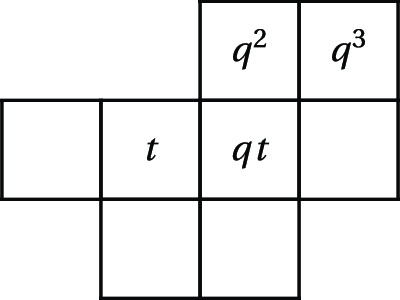
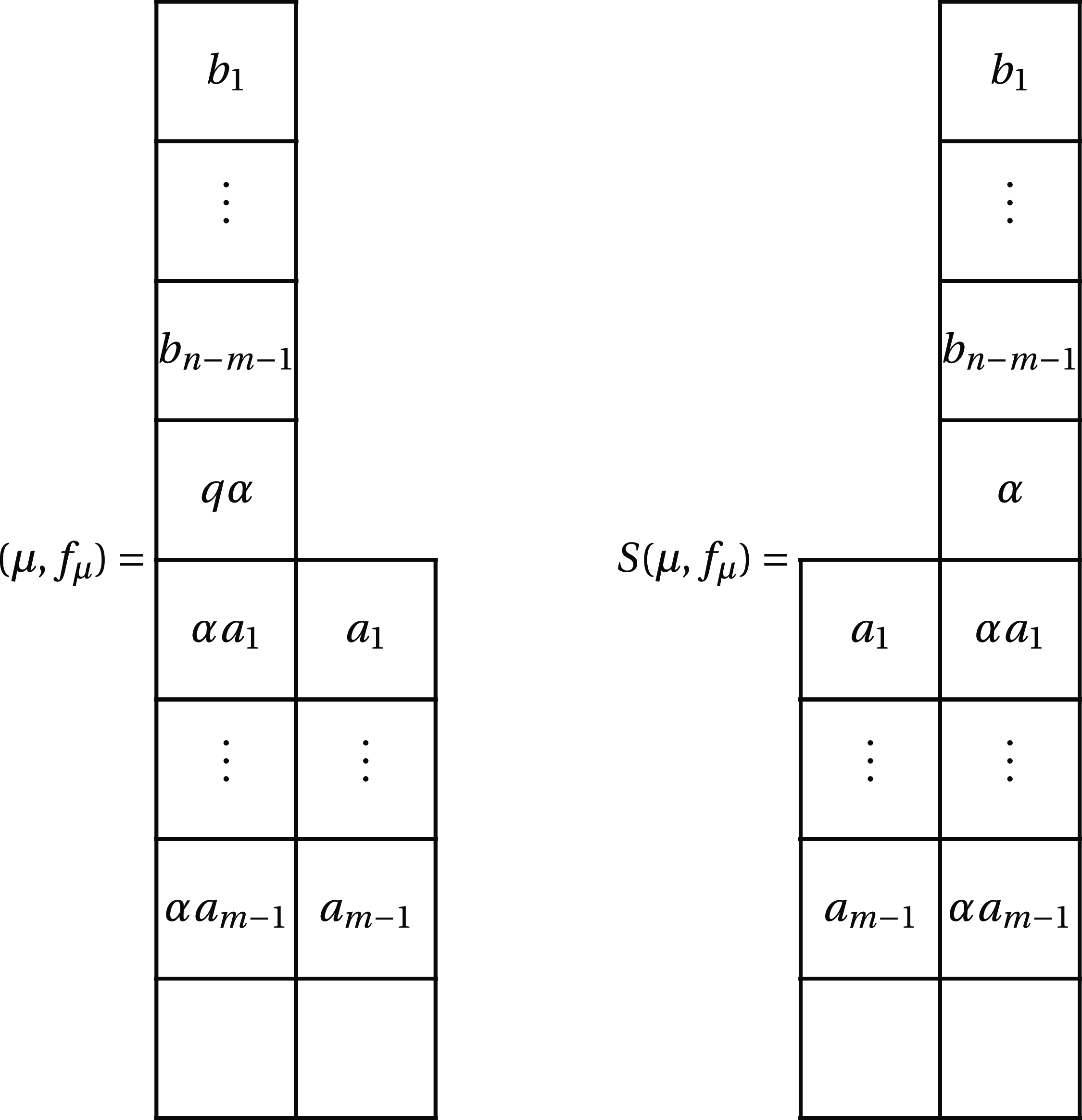
See Figure 4 for an example.
Let
 $(D,f)$
be a filled diagram such that the restriction to the
 $j$
th and
 $(j+1)$
th columns is in
 $\mathcal {V}(n,m)$
for some
 $n\gt m$
. We define
 $S_j(D,f)$
to be the filled diagram obtained from
 $(D,f)$
by applying the map
 $S$
to the two columns (
 $j$
th and
 $(j+1)$
th columns). Clearly, the map
 $S_j$
is injective, so we may consider
 $S_j^{-1}(D,f)$
if it exists. Given two filled diagrams
 $(D,f)$
and
 $(D^{\prime},f^{\prime})$
, we write
 $(D,f)\cong (D^{\prime},f^{\prime})$
if they are related by a sequence of operators of the form
 $S_j$
or
 $S_j^{-1}$
.
The filled diagram
 $(\mu ,f_{\mu })\in \mathcal {V}(n,m)$
is of the form on the left for some
 $a_i$
,
 $b_i$
, and
 $\alpha$
in
 $\mathbb {F}$
. The right figure shows the corresponding
 $S(\mu ,f_{\mu })$
.

Proposition 5.3 [Reference Kim, Lee and OhKLO22, Proposition 4.3 rephrased]. Let
 $(D,f)$
and
 $(D^{\prime},f^{\prime})$
be filled diagrams of size
 $n$
such that
 $(D,f)\cong (D^{\prime},f^{\prime})$
. We let
 $P_{i}$
be the set of
 $N_{D}(u)$
for the cells
 $u$
in the
 $i$
th row of
 $D$
. Then there is a bijection
 $\phi :\mathfrak {S}_n\rightarrow \mathfrak {S}_n$
satisfying the following three conditions:
-
$\mathrm {stat}_{(D,f)}(w) = \mathrm {stat}_{(D^{\prime},f^{\prime})}(\phi (w))$
;
-
$ \mathrm {iDes}(w) = \mathrm {iDes}(\phi (w)) $
;
-
$\{w_{j}: j \in P_i\} = \{\phi (w)_{j}: j \in P_i\} \text { for all }i$
.


With the assumptions in Proposition 5.3, conditions
 $(\phi 1)$
and
 $(\phi 2)$
are enough to imply
 $\widetilde {H}_{(D,f)}[X]=\widetilde {H}_{(D^{\prime},f^{\prime})}[X]$
. However, we need a more refined identity (5.3) coming from the condition
 $(\phi 3)$
that will be used in the proof of Lemma 6.12 and Lemma 6.18. We define some terminology to state (5.3).
Definition 5.4. For diagram
 $D$
and a composition
 $\alpha =(\alpha _1,\dots ,\alpha _{r})$
of size less than or equal to
 $|D|$
, we define
 $\mathrm {OP}(D;\alpha )$
to be the set of tuples
 $(A_1,\dots ,A_{r})$
of disjoint subsets
 $A_i\subseteq D$
such that
 $|A_i|=\alpha _i$
. For a tuple
 $(A_1, \dots , A_{r})\in \mathrm {OP}(D;\alpha )$
, let
 $B_i=\{N_D(u): u\in A_i\}$
where
 $N_D$
is the total order on cells of
 $D$
defined in § 5.1. We define
 $\sigma (D;(A_1, \dots , A_{r}))$
to be the permutation obtained by first listing elements
 $[|D|]\setminus \bigcup\nolimits _{i=1}^{r}B_i$
in decreasing order, followed by elements in
 $B_1$
in decreasing order, then elements in
 $B_2$
in decreasing order, and so on.
For instance, let
 $D = [\{1,2,3,4,5\},\{1,2,3,4\},\{2,3\}]$
be a diagram and
 \begin{equation*} (A_1,A_2,A_3)=(\{(2,2),(3,1),(3,3) \},\{(2,1),(3,2)\}, \{ (2,3),(4,2),(5,1)\})\in \mathrm {OP}(D;(3,2,3)). \end{equation*}
Pictorially,
 $(A_1,A_2,A_3)$
is displayed by labeling cells in
 $A_i$
by
 $i$
as on the leftin Figure 5. According to the total order
 $N_D$
(given on the right in Figure 5), the permutation associated to
 $(A_1,A_2,A_3)$
is
 \begin{equation*} \sigma (D;(A_1,A_2,A_3))=(11,10,2,\underbrace {8,6,4}_{3},\underbrace {7,5}_{2},\underbrace {9,3,1}_{3}). \end{equation*}
An element of
 $\mathrm {OP}(D,(3,2,3))$
and a natural ordering
 $N_{D}$
of
 $D$
.

By (4.3), letting
 $m=|D|-\sum _{i=1}^{r}\alpha _i$
, we have
 \begin{equation} \langle \widetilde {H}_{(D,f)}[X]),e_{(m,\alpha )}\rangle =\sum _{L\in \mathrm {OP}(D;\alpha )}\mathrm {stat}_{(D,f)}(\sigma (D;L)^{-1}). \end{equation}
Now we further refine the set
 $\mathrm {OP}(D;\alpha )$
.
Definition 5.5. Let
 $D$
be a diagram with
 $\ell$
rows. For
 $L=(A_1,\dots ,A_r)\in \mathrm {OP}(D;\alpha )$
, we define an
 $r\times \ell$
matrix
 $\mathrm {type}(D;L)$
by letting its entries be as follows:
 \begin{align*} \mathrm {type}(D;L)_{i,j}=\text {the number of cells in the }j\text {th row of }D\text { that are in }A_i. \end{align*}
Now we define
 $\mathbf {OP}(D;M)$
to be the set of tuples
 $L$
such that
 $\mathrm {type}(D;L)=M$
. Note that
 $\mathrm {rsum}(\mathrm {type}(D;L))=\alpha$
if
 $L\in \mathrm {OP}(D;\alpha )$
. With this notion, we partition
 $\mathrm {OP}(D;\alpha )$
into the union
 \begin{equation*} \mathrm {OP}(D;\alpha )=\bigcup _{\mathrm {rsum}(M)=\alpha }\mathbf {OP}(D;M). \end{equation*}
Given
 $(D,f)\cong (D^{\prime},f^{\prime})$
, let
 $\phi$
be the map in Proposition 5.3. By the conditions
 $(\phi 1)$
and
 $(\phi 2)$
,
 $\phi$
gives a stat-preserving bijection between
 \begin{equation*} \{\sigma (D;L)^{-1}:L\in \mathrm {OP}(D;\alpha )\} \quad \text {and} \quad \{\sigma (D^{\prime};L)^{-1}:L\in \mathrm {OP}(D^{\prime};\alpha )\}. \end{equation*}
Moreover, the condition
 $(\phi 3)$
implies that if
 $\phi (\sigma (D;L)^{-1})=\sigma (D^{\prime};L^{\prime})^{-1}$
, we have
 $\mathrm {type}(D;L)=\mathrm {type}(D^{\prime};L^{\prime})$
. In other words,
 $\phi$
gives a bijection between
 \begin{equation*} \{\sigma (D;L)^{-1}:L\in \mathbf {OP}(D;M)\} \quad \text {and}\quad \{\sigma (D^{\prime};L)^{-1}:L\in \mathbf {OP}(D^{\prime};M)\}. \end{equation*}
We conclude that for any
 $M\in \mathrm {Mat}^{\geq 0}$
,
 \begin{equation} \sum _{L\in \mathbf {OP}(D;M)}\mathrm {stat}_{(D,f)}(\sigma (D;L)^{-1})=\sum _{L\in \mathbf {OP}(D^{\prime};M)}\mathrm {stat}_{(D^{\prime},f^{\prime})}(\sigma (D^{\prime};L)^{-1}). \end{equation}
We end this section by recalling the cycling rule. Given a diagram
 $D=[D^{(1)},\dots ,D^{(\ell )}]$
, consider a diagram
 \begin{equation*} D^{\prime}=[D^{(2)},\dots ,D^{(\ell )},D^{(1)}+1], \end{equation*}
where
 $I+1=\{a+1:a\in I\}$
for an interval
 $I$
. In other words,
 $D^{\prime}$
is a diagram obtained by moving the leftmost column of
 $D$
to the right end and placing it one cell up. Cells in
 $D$
and
 $D^{\prime}$
are naturally in bijection. To a filling
 $f$
of
 $D$
we can associate a filling
 $f^{\prime}$
of
 $D^{\prime}$
inherited from
 $f$
via this natural bijection. Then we define
 $\mathrm {Cyc} (D,f):=(D^{\prime},f^{\prime})$
. Then the following lemma is well known and its proof is straightforward (see [Reference Kim, Lee and OhKLO22, Lemma 3.6], for example).
Lemma 5.6 [Cycling rule]. Let
 $(D,f)$
be a filled diagram and
 $(D^{\prime},f^{\prime})=\mathrm {Cyc}(D,f)$
. Then we have
 \begin{align*} \widetilde {H}_{(D,f)}[X] = \widetilde {H}_{(D^{\prime},f^{\prime})}[X]. \\[-16pt] \end{align*}
6. Lightning bolt formula for Macdonald intersection polynomials
In this section, we present the lightning bolt formula for Macdonald intersection polynomials, which plays a key role in the proof of Theorem 1.1(c). Thanks to the shape independence stated in Theorem 1.1(b), it is sufficient to compute
 $e^{\perp }_{n+1-k}\mathrm {I}_{\mu ^{(1)},\dots ,\mu ^{(k)}}$
for any tuple of distinct partitions
 $(\mu ^{(1)},\dots ,\mu ^{(k)})$
where there exists a partition
 $\mu \vdash n+1$
satisfying
 $|\mu \backslash \mu ^{(i)}|=1$
. In this section, we fix
 $\mu$
as the augmented staircase
 $\overline {\delta }_k:=(\underbrace {k,\dots ,k}_{k},k-1,\dots ,1)$
and
 $\mu ^{(i)}=\overline {\delta }_k\backslash c_i$
, where
 $c_1,\dots ,c_k$
represent removable corners of
 $\overline {\delta }_k$
indexed from top to bottom.
Here, we outline the contents of this section. In § 6.1, we apply the column exchange rule to
 $(\mu ^{(i)},f^{\mathrm {st}}_{\mu ^{(i)}})$
to obtain a filled diagram
 $(\overline {\delta }_{k,i}, \overline {f}_{k,i})$
. In § 6.2, we present the lightning bolt formula for the Macdonald intersection polynomials (Proposition 6.4), which serves as a key component in proving Theorem 1.1(c). In § 6.3, we demonstrate the reduction of Proposition 6.4 to Proposition 6.17. Section 6.4 provides a proof of Proposition 6.17, which finalizes the proof of Theorem 1.1(c).
6.1 Deforming the filled diagram
$(\mu ^{(i)},f^{\mathrm {st}}_{\mu ^{(i)}})$

In this subsection, we introduce a filled diagram
 $(\overline {\delta }_{k,i},\overline {f}_{k,i})$
that possesses the property
 \begin{equation*} \widetilde {H}_{\left(\mu ^{(i)},f^{\mathrm {st}}_{\mu ^{(i)}}\right)}[X]=\widetilde {H}_{\left(\overline {\delta }_{k,i},\overline {f}_{k,i}\right)}[X]. \end{equation*}
For the computation of
 $\mathrm {I}_{\mu ^{(1)},\dots ,\mu ^{(k)}}$
, we will utilize
 $(\overline {\delta }_{k,i},\overline {f}_{k,i})$
in place of
 $(\mu ^{(i)},f^{\mathrm {st}}_{\mu ^{(i)}})$
.
Definition 6.1. We define
 \begin{equation*} \left(\overline {\delta }_{k,i},\overline {f}_{k,i}\right):=\mathrm {Cyc} (S_1\dots S_{i-1}(\mu ^{(i)},f^{\mathrm {st}}_{\mu ^{(i)}}) ). \end{equation*}
Refer to Figure 6 for an illustrative example. In other words, we perform the following procedure: we shift the
 $i$
th column of
 $(\mu ^{(i)},f^{\mathrm {st}}_{\mu ^{(i)}})$
all the way to the left by applying
 $S_1\cdots S_{i-1}$
, and then we take the first column (previously the
 $i$
th column) and move it to the far right using the operator
 $\mathrm {Cyc}$
. It can be verified that the local condition (5.1) is always satisfied during the application of the operators
 $S_1\cdots S_{i-1}$
. For a detailed proof, we refer to [Reference Kim, Lee and OhKLO22, Lemma 5.2].
Lemma 6.2. We have
 $\overline {\delta }_{k,i}=[I_1,I_2,\dots ,I_k]$
, where
 $I_j$
is the interval given by
 \begin{equation*} I_j = \begin{cases} [2k-j] &\text {if } j\lt i, \\ [2k-j-1] &\text {if } i\le j\lt k, \\ [2,2k-i] &\text {if } j=k. \end{cases} \end{equation*}
The filling
 $\overline {f}_{k,i}$
on
 $\overline {\delta }_{k,i}$
is given by
 \begin{align*} \overline {f}_{k,i}(a,b) = \begin{cases} q^{b-k}t^{2k-a-b+1}&\text {if } a\le k \ \mathrm{ and }\ b\lt i,\\ q^{b-k+1}t^{2k-a-b}&\text {if } a\le k\ \mathrm{ and }\ i\le b\lt k,\\ q^{i-k} t^{2k-i-a+1}&\text {if } a\le k\ \mathrm{ and }\ b=k,\\ q^{a+b-2k}t^{2k-a-b+1}&\text {if } a\gt k\ \mathrm{ and }\ b\lt i,\\ q^{a+b-2k+1}t^{2k-a-b}&\text {if } a\gt k\ \mathrm{ and }\ i\le b \lt k,\\ q^{i+a-2k-1}t^{2k-i-a+1}&\text {if } a\gt k\ \mathrm{ and }\ b=k. \end{cases} \\[-12pt] \end{align*}
The figure on the left depicts the filled diagram
 $(\mu ^{(3)},f^{\mathrm {st}}_{\mu ^{(3)}})$
, while the one in the center represents the filled diagram
 $S_1 S_2(\mu ^{(3)},f^{\mathrm {st}}_{\mu ^{(3)}})$
. Finally, the figure on the right illustrates the filled diagram
 $(\overline {\delta }_{4,3}, \overline {f}_{4,3})$
, which is obtained by applying the operator
 $\mathrm {Cyc}$
to the figure in the center.

Proof. The standard filling of
 $\mu ^{(i)}$
is given by
 \begin{align*} f^{\mathrm {st}}_{\mu ^{(i)}}(a,b)= \begin{cases} q^{b-k}t^{2k-a-b+1}&\text {if } a\le k\mbox{ and } b\neq i,\\ q^{i-k}t^{2k-a-i}&\text {if } a\le k\mbox{ and } b= i,\\ q^{a+b-2k}t^{2k-a-b+1}&\text {if } k\lt a\lt 2k-i\mbox{ and } b\neq i\text { or }a\gt 2k-i,\\ q^{a+i-2k}t^{2k-a-i}&\text {if } a\gt k\mbox{ and } b=i,\\ q^{b-i+1}t^{i-b+1}&\text {if } a=2k-i. \end{cases} \\[-12pt] \end{align*}
While applying the operator
 $S_1\dots S_{i-1}$
, the only changes of the filling occur in the
 $(2k-i)$
th row upon multiplying by
 $q^{-1}$
. Writing
 $(D,f)=S_1\dots S_{i-1}(\mu ^{(i)},f^{\mathrm {st}}_{\mu ^{(i)}})$
, we have
 \begin{equation*} D = [[2k-i-1],[2k-1],\dots ,[2k-i+1],[2k-i-1],\dots ,[k]] \end{equation*}
and
 \begin{align*} f(a,b)= \begin{cases} q^{i-k} t^{2k-a-i}&\text {if } a\le k\mbox{ and } b=1,\\ q^{b-k-1}t^{2k-a-b+2}&\text {if } a\le k\mbox{ and } 1\lt b\le i,\\ q^{b-k}t^{2k-a-b+1}&\text {if } a\le k\mbox{ and } b\gt i,\\ q^{a+i-2k}t^{2k-a-i}&\text {if } a\gt k\mbox{ and } b=1,\\ q^{a+b-2k-1}t^{2k-a-b+2}&\text {if } a\gt k\mbox{ and } 1\lt b\le i,\\ q^{a+b-2k}t^{2k-a-b+1}&\text {if } a\gt k\mbox{ and } b\gt i. \end{cases} \\[-12pt] \end{align*}
Applying the operator
 $\mathrm {Cyc}$
completes the proof.
Remark 6.3. Let
 $\lambda$
be a partition and
 $(D,f)$
a filled diagram satisfying
 $(D,f)\cong (\lambda ,f_{\lambda }^{\mathrm {st}})$
. Then [Reference Haglund, Haiman and LoehrHHL08, Theorem 5.1.1] implies
 $\widetilde {H}_{(D,f)}[X]=\widetilde {H}_{(\lambda ,f^{\mathrm {st}}_{\lambda })}[X]$
. In particular, letting
 $(D,f)=S_{1}\dots S_{i-1}(\mu ^{(i)},f^{\mathrm {st}}_{\mu ^{(i)}})$
, we obtain
 \begin{equation*} \widetilde {H}_{(D,f)}[X]=\widetilde {H}_{\left(\mu ^{(i)},f^{\mathrm {st}}_{\mu ^{(i)}}\right)}[X] \end{equation*}
without using Proposition 5.3. However, [Reference Haglund, Haiman and LoehrHHL08, Theorem 5.1.1] is not enough for our purposes later when we deal with
 $z$
-deformed filled diagrams in § 6.3. Moreover, we need a more refined identity (5.3).
6.2 Lightning bolt formula for Macdonald intersection polynomials
In this subsection, we state the lightning bolt formula for Macdonald intersection polynomials (Proposition 6.4), which essentially proves Theorem 1.1(c).
By (5.2), for a composition
 $\beta \models k-1$
we have
 \begin{align} \langle e^{\perp }_{n+1-k}\mathrm {I}_{\mu ^{(1)},\dots ,\mu ^{(k)}}[X;q,t],e_{\beta }\rangle &=\sum _{i=1}^{k} \bigg (\prod _{j\neq i}\dfrac {T_{\mu ^{(j)}}}{T_{\mu ^{(j)}}-T_{\mu ^{(i)}}}\bigg )\sum _{L\in \mathrm {OP}(\overline {\delta }_{k,i};\beta )}\mathrm {stat}_{(\overline {\delta }_{k,i},\overline {f}_{k,i})} (\sigma (\overline {\delta }_{k,i};L)^{-1} )\nonumber \\ &=\sum _{\substack {M\in \mathrm {Mat}^{\ge 0}_{r\times (2k-1)} \nonumber \\\mathrm {rsum}(M)=\beta }}\sum _{i=1}^{k} \bigg (\prod _{j\neq i}\dfrac {T_{\mu ^{(j)}}}{T_{\mu ^{(j)}}-T_{\mu ^{(i)}}}\bigg )\sum _{L\in \mathbf {OP}(\overline {\delta }_{k,i};M)}\nonumber \\[5pt]&\mathrm {stat}_{(\overline {\delta }_{k,i},\overline {f}_{k,i})} (\sigma (\overline {\delta }_{k,i};L)^{-1} ).\end{align}
Now we present the remarkable observation which we refer to as the lightning bolt formula for Macdonald intersection polynomials. This formula establishes a connection between the Macdonald intersection polynomial and the fermionic formula for the shuffle formula (Theorem 4.6). The next subsections are devoted to a proof of Proposition 6.4.
Proposition 6.4. For
 $M\in \mathrm {Mat}^{\ge 0}_{r\times (2k-1)}$
such that
 $|M|=k-1$
, writing
 $\alpha =\mathrm {csum}(M)$
, we have
 \begin{align*} & \sum _{i=1}^{k} \bigg (\prod _{j\neq i}\dfrac {T_{\mu ^{(j)}}}{T_{\mu ^{(j)}}-T_{\mu ^{(i)}}}\bigg )\sum _{L\in \mathbf {OP}(\overline {\delta }_{k,i};M)}\mathrm {stat}_{(\overline {\delta }_{k,i},\overline {f}_{k,i})} (\sigma (\overline {\delta }_{k,i};L)^{-1} )\\[6pt]&\qquad =T_{\bigcap _{i=1}^k \mu ^{(i)}}(t^{\sum _{i=1}^{\ell (\alpha )}(i-1)\alpha _i}q^{\sum _{i,j} \binom {M_{i,j}}{2}} ) \mathrm {lb}(M). \end{align*}
We end this subsection with a proof of Theorem 1.1(c) assuming Proposition 6.4.
Proof of Theorem
1.1(c). For any
 $\beta \models k-1$
, by Proposition 6.4 and (6.1) we have
 \begin{equation*} \bigg\langle \dfrac {1}{T_{\bigcap _{i=1}^k \mu ^{(i)}}}e_{n+1-k}^\perp \left (\mathrm {I}_{\mu ^{(1)},\dots ,\mu ^{(k)}}[X;q,t]\right ),\:e_{\beta }\bigg\rangle =\sum _{\alpha }\sum _{\substack {M\in \mathrm {Mat}^{\ge 0}_{\ell (\beta )\times (2k-1)}\\ \mathrm {csum}(M)=\alpha \\ \mathrm {rsum}(M)=\beta }}(t^{\sum _{i=1}^{\ell (\alpha )}(i-1)\alpha _i}q^{\sum _{i,j} \binom {M_{i,j}}{2}} ) \mathrm {lb}(M), \end{equation*}
where the sum on the right-hand side is over vectors
 $\alpha$
of length
 $2k-1$
whose entries are nonnegative integers. By applying Lemma 4.5, we can deduce that if
 $\mathrm {csum}(M)$
is not in the form of
 $(\alpha ^{\prime},0,\dots ,0)$
for a composition
 $\alpha ^{\prime}\models k-1$
, then
 $\mathrm {lb}(M)=0$
. Consequently, our focus narrows down to matrices where
 $\mathrm {csum}(M)$
takes the form
 $(\alpha ^{\prime},0,\dots ,0)$
for some
 $\alpha ^{\prime}\models k-1$
. Using Theorem 4.6, we can finally conclude that
 \begin{equation*} \bigg\langle \dfrac {1}{T_{\bigcap _{i=1}^k \mu ^{(i)}}}e_{n+1-k}^\perp \left (\mathrm {I}_{\mu ^{(1)},\dots ,\mu ^{(k)}}[X;q,t]\right )\!, \:e_{\beta }\bigg\rangle =\langle D_{k-1}[X;q,t],\,e_{\beta }\rangle \end{equation*}
for any
 $\beta \models k-1$
, which is enough to deduce that
 \begin{equation*} \dfrac {1}{T_{\bigcap _{i=1}^k \mu ^{(i)}}}e_{n+1-k}^\perp \left (\mathrm {I}_{\mu ^{(1)},\dots ,\mu ^{(k)}}[X;q,t]\right )=D_{k-1}[X;q,t]. \end{equation*}
Our current objective is to prove Proposition 6.4. In § 6.3, we will demonstrate that it is sufficient to establish Proposition 6.17, the proof of which will be provided in § 6.4.
6.3 Reducing to the rectangular case
We first introduce a
 $z$
-deformation
 $(\overline {\delta }_{k,i},\overline {f}^{\mathbf {z}}_{k,i})$
of the filled diagram
 $(\overline {\delta }_{k,i},\overline {f}_{k,i})$
, where the filling
 $\overline {f}_{k,i}^{\textbf {z}}$
on
 $\overline {\delta }_{k,i}$
is defined as follows:
 \begin{equation} \overline {f}_{k,i}^{\textbf {z}}(a,b) = \begin{cases} q z_{2k+1-a}/z_b &\text {if } b\lt i, \\[3pt] q z_{2k+1-a}/z_{b+1} &\text {if } i\le b\lt k,\\[3pt] q z_{2k+1-a}/z_i &\text {if } a\le k\mbox{ and } b=k,\\[3pt] z_{2k+1-a}/z_i &\text {if } a\gt k\mbox{ and } b=k. \end{cases} \end{equation}
Figure 7 shows
 $(\overline {\delta }_{4,3},\overline {f}_{4,3}^{\textbf {z}})$
, which is a
 $z$
-deformation of
 $(\overline {\delta }_{4,3},\overline {f}_{4,3})$
shown on the right of Figure 6.
A
 $z$
-deformed filled diagram
 $(\overline {\delta }_{4,3},\overline {f}_{4,3}^{\textbf {z}})$
.

By Lemma 6.2, one can directly see that substituting
 \begin{equation} z_j = \begin{cases} q^{1-j}t^{j-1}&\text {if } j\le k,\\[3pt] q^{-k}t^{j-1}&\text {if } j \gt k \end{cases} \end{equation}
recovers
 $(\overline {\delta }_{k,i}\overline {f}_{k,i})$
. We now introduce a
 $z$
-deformed version of Proposition 6.4.
Proposition 6.5. For
 $M\in \mathrm {Mat}^{\ge 0}_{r\times (2k-1)}$
such that
 $|M|=k-1$
, letting
 $\alpha =\mathrm {csum}(M)$
, we have
 \begin{align*} & \sum _{i=1}^{k} \bigg (\prod _{j\neq i}\dfrac {z_j}{z_j-z_i}\bigg )\sum _{L\in \mathbf {OP}(\overline {\delta }_{k,i};M)}\mathrm {stat}_{(\overline {\delta }_{k,i},\overline {f}^{\mathbf {z}}_{k,i})} (\sigma (\overline {\delta }_{k,i};L)^{-1} )\\[5pt]&\quad =q^{({4k^3-6k^2-k})/{3}+\sum _{i,j}\binom {M_{i,j}}{2}}\bigg(\frac {z_k\prod _{i=1}^{k-1}z_{2k-i}^{k-\alpha _i}}{z_{2k-1}\prod _{i=1}^{k-1}z_i^{2k-2i-1} }\bigg) \mathrm {lb}(M). \end{align*}
On the right-hand side, we may consider only
 $\alpha$
such that
 $\alpha _\ell =0$
for
 $\ell \geq k$
(otherwise
 $\mathrm {lb}(M)=0$
), and a simple computation shows that
 \begin{align*} \frac {T_{\mu ^{(i)}}}{T_{\mu ^{(j)}}}=\frac {z_i}{z_j},\quad q^{({4k^3-6k^2-k})/{3}}\bigg(\frac {z_k\prod _{i=1}^{k-1}z_{2k-i}^{k-\alpha _i}}{z_{2k-1}\prod _{i=1}^{k-1}z_i^{2k-2i-1} }\bigg)=T_{\bigcap _{i=1}^k \mu ^{(i)}}(t^{\sum _{i=1}^{k-1}(i-1)\alpha _i}) \end{align*}
under the specialization (6.3). Therefore Proposition 6.4 follows from Proposition 6.5. We will reduce Proposition 6.5 to Proposition 6.17, which analyzes the rectangular case. Here is the outline of the strategy.
-
(1) We first establish the equivalence between Proposition 6.5 and (6.6) by introducing a complementary statistic
$\overline {\mathrm {stat}}$
(Definition 6.6). -
(2) We restrict our attention to the almost rectangular shape
$\overline {R}_{k}$
in the first
$k$
rows (shown on the left in Figure 8), utilizing Lemma 6.11 and Lemma 6.12. This reduction transforms (6.6) into (6.12). -
(3) We establish a connection between the rectangular shape
$R_k$
(on the right in Figure 8) and
$\overline {R_k}$
in Lemma 6.16. -
(4) We present Proposition 6.17 and demonstrate that when combined with Lemma 6.16 and Lemma A.1, it completes the proof of Proposition 6.5.


Definition 6.6. Given a filled diagram
 $(D,f)$
, let
 $L=(A_1,\dots ,A_r)\in \mathbf {OP}(D;M)$
for some
 $M\in \mathrm {Mat}^{\geq 0}$
. We set
 $A_0=D\setminus \bigcup _{i=1}^r A_i$
, so that for every cell
 $u\in D$
there exists unique
 $\ell$
such that
 $u\in A_{\ell }$
. We define
 $\overline {\mathrm {Inv}}_D(L)$
as the set of attacking pairs
 $(u,v)$
that do not belong to
 $\mathrm {Inv}_D(\sigma (D;L)^{-1})$
. In other words,
 $\overline {\mathrm {Inv}}_D(L)$
consists of pairs
 $(u,v)$
of cells in
 $D$
such that
 $(u,v)$
is an attacking pair and
 $u$
belongs to
 $A_{\ell }$
while
 $v$
belongs to
 $A_{\ell ^{\prime}}$
with
 $ \ell \lt \ell ^{\prime}$
. We define
 $\overline {\mathrm {inv}}_D(L)$
as the product of
 $q$
over all pairs
 $(u,v)\in \overline {\mathrm {Inv}}_D(L)$
.
Next, we define
 $\overline {\mathrm {Des}}_D(L)$
as the set of cells in
 $D$
that are not bottom cells and are not in
 $\mathrm {Des}_D(\sigma (D;L)^{-1})$
. In other words,
 $\overline {\mathrm {Des}}_D(L)$
consists of cells
 $(i,j)$
in
 $D$
such that
 $(i,j)\in A_{\ell }$
and
 $(i-1,j)\in A_{\ell ^{\prime}}$
for
 $\ell \lt \ell ^{\prime}$
, where
 $A_0$
is defined as before. We let
 $\overline {\mathrm {maj}}_{(D,f)}(L)$
denote the product of
 $f(u)$
over all cells
 $u\in \overline {\mathrm {Des}}_D(L)$
. Finally, we define
 $\overline {\mathrm {stat}}_{(D,f)}$
as follows:
 \begin{equation*} \overline {\mathrm {stat}}_{(D,f)}(L) := \overline {\mathrm {inv}}_{D}(L)\overline {\mathrm {maj}}_{(D,f)}(L). \end{equation*}
By definition, we have
 \begin{equation*} \mathrm {stat}_{(D,f)}(\sigma (D;L)^{-1})=\frac {\mathrm {stat}_{(D,f)}(w_0)}{\overline {\mathrm {stat}}_{(D,f)}(L)}=\frac {\mathrm {stat}_{(D,f)}(w_0)}{\overline {\mathrm {inv}}_D(L)\overline {\mathrm {maj}}_{D,f}(L)}, \end{equation*}
where
 $w_0$
is the longest permutation in
 $\mathfrak {S}_{|D|}$
.
Lemma 6.7. For each
 $1\le i\le k$
,
 \begin{equation*} \mathrm {stat}_{(\overline {\delta }_{k,i},\overline {f}_{k,i}^{\textbf {z}})}(w_0)= q^{({4k^3-3k^2-4k})/{3}}\dfrac {z_i\prod _{j=1}^{k-1}z_{2k-j}^k}{z_{2k-1}\prod _{j=1}^{k-1}z_j^{2k-2j}} \end{equation*}
for the longest permutation
 $w_0$
.
Proof. For simplicity, let
 $(D,f)=(\overline {\delta }_{k,i},\overline {f}_{k,i})$
. We claim that
 \begin{equation} \mathrm {maj}_{(D,f)}(w_0) = q^{(({3k^2-5k})/{2}) + i-1}\dfrac {z_i\prod _{j=1}^{k-1}z_{2k-j}^k}{z_{2k-1}\prod _{j=1}^{k-1}z_j^{2k-2j}} \end{equation}
and
 \begin{equation} \mathrm {inv}_{D}(w_0) = q^{(({8k^3-15k^2+7k})/{6})+1-i}, \end{equation}
which completes the proof.
The first claim, (6.4), follows directly from the definition of
 $\overline {f}_{k,i}$
in (6.2) and the fact that
 $\mathrm {maj}_{(D,f)}(w_0)=\prod _{c\in D}\overline {f}_{k,i}(c)$
. To see (6.5), note that for a given cell
 $u=(a,b)$
, the number of pairs
 $(u,v)$
in attacking position in
 $D$
is
 \begin{equation*} \begin{cases} k-1 &\text { if } 1\lt a\le k\mbox{ and } 1\le b \le k,\\ k-b-1 &\text { if } a=1\mbox{ and } 1\le b\lt k,\\ 2k-a-1 &\text { if } k\lt a\le 2k-i\mbox{ and } 1\le b\le 2k-a-1 \text { or if } 2k-i\lt a\lt 2k\mbox{ and } 1\le b\le 2k-a,\\ 2k-a &\text { if } k\lt a\le 2k-i\mbox{ and } b=k.\\ \end{cases} \end{equation*}
Therefore, the total number of such attacking pairs, i.e. the total number of inversion pairs of
 $w_0$
, is
 \begin{align*} & k(k-1)^2 + \sum _{1\le b \lt k}(k-b-1) + \sum _{k\lt a\le 2k-i}(2k-a-1)^2 + \sum _{2k-i\lt a\lt 2k}(2k-a-1)(2k-a) \\[6pt]&\qquad + \sum _{k\lt a\le 2k-i}(2k-a)\\&\quad = \frac {8k^3-15k^2+7k}{6}+1-i. \end{align*}
By the above lemma, the term
 $(\prod _{j\neq i}z_j)\mathrm {stat}_{(\overline {\delta }_{k,i},\overline {f}_{k,i}^{\textbf {z}})}(w_0)$
is independent of
 $i$
, so the left-hand side of Proposition 6.5 becomes
 \begin{align*} q^{\frac {4k^3-3k^2-4k}{3}}\dfrac {z_k\prod _{j=1}^{k-1}z_{2k-j}^k}{z_{2k-1}\big (\prod _{j=1}^{k-1}z_j^{2k-2j-1}\big ) }\sum _{i=1}^{k} \bigg(\prod _{j\neq i}\dfrac {1}{z_j-z_i}\bigg)\sum _{L\in \mathbf {OP}(\overline {\delta }_{k,i};M)}\frac {1}{\overline {\mathrm {stat}}_{(\overline {\delta }_{k,i},\overline {f}^{\mathbf {z}}_{k,i})}(L)}. \end{align*}
Therefore, after the cancellation, Proposition 6.5 is equivalent to the following: for
 $M\in \mathrm {Mat}^{\ge 0}_{r\times (2k-1)}$
such that
 $|M|=k-1$
, letting
 $\alpha =\mathrm {csum}(M)$
, we have
 \begin{equation} \sum _{i=1}^{k} \bigg(\prod _{j\neq i}\dfrac {1}{z_j-z_i}\bigg)\sum _{L\in \mathbf {OP}(\overline {\delta }_{k,i};M)}\frac {1}{\overline {\mathrm {stat}}_{(\overline {\delta }_{k,i},\overline {f}^{\mathbf {z}}_{k,i})}(L)}=\bigg(\frac {q^{\sum _{i,j}\binom {M_{i,j}}{2}}}{q^{k(k-1)}\prod _{i=1}^{k-1}z_{2k-i}^{\alpha _i}}\bigg)\mathrm {lb}(M). \end{equation}
Now we analyze (6.6). Before doing so, we define some terminology and prove preparatory lemmas (Lemmas 6.11 and 6.12).
For a diagram
 $D$
, note that
 $\mathbf {OP}(D;M)$
makes sense if
 $M$
has
 $\ell$
columns where
 $\ell$
is the number of rows in
 $D$
. For a matrix
 $M$
with
 $\ell ^{\prime}$
columns such that
 $\ell ^{\prime}\lt \ell$
, we consider
 $\overline {M}$
obtained by appending
 $\ell -\ell ^{\prime}$
zero columns to
 $M$
. From now on, with an abuse of notation, we refer to
 $\mathbf {OP}(D;\overline {M})$
as
 $\mathbf {OP}(D;M)$
.
Let
 $D$
be a diagram and
 $E$
a subdiagram of
 $D$
. Given
 $L=(A_1,\dots ,A_r)\in \mathbf {OP}(D;M)$
, we define
 $L \vert _E$
as
 $(A_1 \cap E,\dots ,A_r \cap E)$
.
Definition 6.8. We define the diagram
 $\overline {R}_k$
to be the subdiagram of
 $\overline {\delta }_{k,i}$
obtained by restricting to the first
 $k$
rows and the diagram
 $R_k$
to be the subdiagram of
 $\overline {R}_k$
obtained by restricting to the first
 $k-1$
columns. In other words,
 $\overline {R}_k=[I_1,I_2,\dots ,I_k]$
and
 $R_k=[I_1,I_2,\dots ,I_{k-1}]$
, where
 $I_j$
is the interval given by
 \begin{equation*} I_j = \begin{cases} [k] & \text {if } j\lt k,\\ [2,k] & \text {if } j=k. \end{cases} \end{equation*}
We define
 $(\overline {R}_{k},\overline {g}^{\mathbf {z}}_{k,i})$
and
 $(R_{k},g_{k,i}^{\mathbf {z}})$
to be corresponding sub-filled diagrams of
 $(\overline {\delta }_{k,i},\overline {f}^{\mathbf {z}}_{k,i})$
.
To describe the filling
 $\overline {g}^{\mathbf {z}}_{k,i}$
, it is convenient to introduce the following operator.
Definition 6.9. For a function
 $P(z_1,\dots ,z_{k-1})$
of variables
 $z_1,\dots ,z_{k-1}$
, let
 $\eta _{k,i}$
be the operator that shifts the indices of variables by
 \begin{equation*} \eta _{k,i}\left (P(z_1,\dots ,z_{k-1})\right ):= P(z_1,\dots ,z_{i-1},z_{i+1},\dots ,z_{k}). \end{equation*}
Using the operator
 $\eta _{k,i}$
, we can write the filling
 $\overline {g}^{\mathbf {z}}_{k,i}$
of
 $\overline {R}_k$
as
 \begin{equation*} \overline {g}^{\mathbf {z}}_{k,i}(a,b)= \begin{cases} \eta _{k,i}\bigg(\dfrac {q(z_{2k+1-a})}{z_b}\bigg) &\text{if } b\lt k, \\[12pt]\dfrac {q(z_{2k+1-a})}{z_i} &\text {if } b=k. \end{cases} \end{equation*}
For example, recall the filled diagram
 $(\overline {\delta }_{4,3},\overline {f}_{4,3}^{\textbf {z}})$
in Figure 7. Taking the sub-filled diagram by restricting to the first four rows, we obtain the filled diagram
 $(\overline {R}_{4},\overline {g}^{\mathbf {z}}_{4,3})$
(on the left in Figure 8). Again by restricting to the first three columns, we obtain the filled diagram
 $({R}_{4},g^{\mathbf {z}}_{4,3})$
(on the right in Figure 8).
The filled diagrams
 $(\overline {R}_{4},\overline {g}^{\mathbf {z}}_{4,3})$
and
 $({R}_{4},{g}_{4,3}^{\mathbf {z}})$
.

Definition 6.10. Let
 $D$
be a diagram which is
 $\overline {R}_k$
or
 $R_k$
and consider
 $L=(A_1,\dots ,A_r)\in \mathbf {OP}(D;M)$
, where
 $ M\in \mathrm {Mat}^{\ge 0}_{r\times (k-1)}$
. We define a vector
 $\gamma (D;L)$
of length
 $k-1$
, whose
 $i$
th component is the number of cells
 $c\in \bigcup _{1\le j \le r}A_j$
that belong to the
 $i$
th row of
 $D$
and are such that the cell
 $c^{\prime}$
right above
 $c$
does not belong to
 $\overline {\mathrm {Des}}_D(L)$
. In other words,
 $c\in A_j$
and
 $c^{\prime}\in A_{j^{\prime}}$
for
 $j \leq j^{\prime}$
. It is worth noting that there is no cell
 $c\in \bigcup _{1\le j \le r}A_j$
that is in the
 $k$
th row of
 $D$
as the matrix
 $M$
has
 $k-1$
columns. We say that
 $L$
is reduced with respect to
 $D$
if
 $\gamma (D;L)=0$
. The set of reduced elements in
 $\mathbf {OP}(D;M)$
is denoted by
 $\mathbf {OP}^{\mathrm {red}}(D;M)$
.
For instance, consider the diagram
 $D=\overline {R}_4$
and
 $L$
and
 $L^{\prime}$
depicted in Figure 9. In this example,
 $L$
is reduced, while
 $L^{\prime}$
is not reduced since
 $\gamma (D;L^{\prime})=(1,1,0)$
(the cells contributing to
 $\gamma (D;L^{\prime})$
are shaded in gray).
The following two lemmas will be used to transform (6.6) to (6.12), which only concerns the reduced elements in
 $\mathbf {OP}(D;M)$
.
On the left is
 $L$
, which is reduced, while
 $L^{\prime}$
on the right is not reduced.

Lemma 6.11. Let
 $M\in \mathrm {Mat}^{\ge 0}_{r\times (k-1)}$
and let
 $\gamma$
be a vector of nonnegative integers of length
 $k-1$
. Furthermore, assume that
 $|M|-|\gamma |\lt k-1$
. Then we have
 \begin{equation*} \sum _{i=1}^{k}\bigg(\prod _{j\neq i}\frac {1}{z_j-z_i}\bigg)\sum _{\substack {L\in \mathbf {OP}(\overline {R}_k;M)\\ \gamma (\overline {R}_k;L)=\gamma }}\frac {1}{\overline {\mathrm {stat}}_{(\overline {R}_k,\overline {g}^{\mathbf {z}}_{k,i})}(L)}=0. \end{equation*}
Proof. Let
 $\alpha =\mathrm {csum}(M)$
and
 $L\in \mathbf {OP}(\overline {R}_k;M)$
such that
 $\gamma (\overline {R}_k;L)=\gamma$
. For each
 $1\leq j\leq k-1$
, there are exactly
 $\alpha _j-\gamma _j$
cells in the
 $(j+1)$
th row of
 $\overline {R}_k$
that are in
 $\overline {\mathrm {Des}}_{\overline {R}_k}(L)$
. Note that if
 $c$
is a cell in the
 $(j+1)$
th row of
 $\overline {R}_k$
, we have
 $\overline {g}^{\mathbf {z}}_{k,i}(c)=q({z_{2k-j}})/{z_{\ell }}$
for some
 $1\leq \ell \leq k$
. Therefore we can write
 \begin{equation} \sum _{\substack {L\in \mathbf {OP}(\overline {R}_k;M) \\ \gamma (\overline {R}_k;L)=\gamma }}\frac {1}{\overline {\mathrm {stat}}_{(\overline {R}_k,\overline {g}_{k,i})}(L)}=\frac {P_i(z_1,\dots ,z_k)}{\prod _{j=1}^{k-1}z_{2k-j}^{\alpha _j-\gamma _j}} \end{equation}
for some polynomial
 $P_i(z_1,\dots ,z_k)$
of degree
 $\sum (\alpha _i-\gamma _i)=|M|-|\gamma |\lt k-1$
. As we have
 $P_i=P_j$
when
 $z_i=z_j$
due to the description of the fillings
 $\overline {g}^{\mathbf {z}}_{k,i}$
and
 $\overline {g}^{\mathbf {z}}_{k,j}$
, Lemma A.2 finishes the proof.
Lemma 6.12. Let
 $M\in \mathrm {Mat}^{\ge 0}_{r\times (2k-1)}$
and write
 $\mathrm {csum}(M)=\alpha$
. If there exists
 $\ell \leq k-1$
such that
 $\alpha _{\ell }=0$
and
 $\sum _{i=1}^{\ell -1}\alpha _i\lt k-1$
, we have
 \begin{equation} \sum _{i=1}^{k}\bigg (\prod _{j\neq i}\frac {1}{z_j-z_i}\bigg )\sum _{\substack {L\in \mathbf {OP}(\overline {\delta }_{k,i};M)}}\frac {1}{\overline {\mathrm {stat}}_{(\overline {\delta }_{k,i},\overline {f}^{\mathbf {z}}_{k,i})}(L)}=0. \end{equation}
Proof. Let
 $(D^{(1)},f^{(1)}_i)$
be the sub-filled diagram of
 $(\overline {\delta }_{k,i},\overline {f}^{\mathbf {z}}_{k,i})$
obtained by restricting to the first
 $\ell$
rows, and let
 $(D^{(2)}_i,f^{(2)}_i)$
be the remaining sub-filled diagram from the
 $(\ell +1)$
th row and above. Note that the shape
 $D^{(1)}$
is independent of
 $i$
. For
 $L=(A_1,\dots ,A_r)\in \mathbf {OP}(\overline {\delta }_{k,i};M)$
, there is no cell in the
 $\ell$
th row that is in
 $\bigcup\nolimits _{t=1}^{r}A_t$
as
 $\alpha _{\ell }=0$
. Therefore we have
 \begin{align*} \overline {\mathrm {Inv}}_{\overline {\delta }_{k,i}}(L)=\overline {\mathrm {Inv}}_{D^{(1)}}(L\vert _{D^{(1)}}) \cup \overline {\mathrm {Inv}}_{D^{(2)}_i}(L\vert _{D^{(2)}_i}), \quad \overline {\mathrm {Des}}_{\overline {\delta }_{k,i}}(L)=\overline {\mathrm {Des}}_{D^{(1)}}(L\vert _{D^{(1)}}) \cup \overline {\mathrm {Des}}_{D^{(2)}_i}(L\vert _{D^{(2)}_i}), \end{align*}
which gives
 $\overline {\mathrm {stat}}_{(\overline {\delta }_{k,i},\overline {f}^{\mathbf {z}}_{k,i})}(L)=\overline {\mathrm {stat}}_{(D^{(1)},f^{(1)}_i)}(L\vert _{D^{(1)}})\overline {\mathrm {stat}}_{(D^{(2)}_i,f^{(2)}_i)}(L\vert _{D^{(2)}_i})$
. Note that we have
 $\mathrm {type}(D^{(1)};L\vert _{D^{(1)}})=M^{(1)}$
and
 $\mathrm {type}(D^{(2)}_i;L\vert _{D^{(2)}_i})=M^{(2)}$
. Here,
 $M^{(1)}$
represents the sub-matrix of
 $M$
obtained by restricting it to the first
 $\ell$
columns. Similarly,
 $M^{(2)}$
is the sub-matrix of
 $M$
obtained by restricting it from the
 $(\ell +1)$
th column to the
 $(2k-1)$
th column. We conclude that
 \begin{align*} & \sum _{L\in \mathbf {OP}(\overline {\delta }_{k,i};M)}\frac {1}{\overline {\mathrm {stat}}_{(\overline {\delta }_{k,i},\overline {f}^{\mathbf {z}}_{k,i})}(L)} \\&\quad =\sum _{L^{(1)}\in \mathbf {OP}(D^{(1)};M^{(1)})}\frac {1}{ \overline {\mathrm {stat}}_{(D^{(1)},f^{(1)}_i)}(L^{(1)})}\sum _{L^{(2)}\in \mathbf {OP}(D^{(2)}_i;M^{(2)})}\frac {1}{ \overline {\mathrm {stat}}_{(D^{(2)}_i,f^{(2)}_i)}(L^{(2)})}. \end{align*}
For
 $1\leq i,j\leq k$
, we have
 \begin{equation*} S_{i}^{-1}\dots S_{k-1}^{-1}(D_{i}^{(2)},f_{i}^{(2)})=S_{j}^{-1}\dots S_{k-1}^{-1}(D_{j}^{(2)},f_{j}^{(2)}), \end{equation*}
which gives
 $(D_{i}^{(2)},f_{i}^{(2)})\cong (D_{j}^{(2)},f_{j}^{(2)})$
. From the identity
 $\widetilde {H}_{(D_{i}^{(2)},f_{i}^{(2)})}[X]=\widetilde {H}_{(D_{j}^{(2)},f_{j}^{(2)})}[X]$
, taking the coefficient of
 $F_{(1,\dots ,1)}$
gives
 \begin{equation} \mathrm {stat}_{(D_{i}^{(2)},f_{i}^{(2)})}(w_0)=\mathrm {stat}_{(D_{j}^{(2)},f_{j}^{(2)})}(w_0) \end{equation}
where
 $w_0$
is the longest permutation of the size
 $|D^{(2)}_i|$
. We also have
 \begin{equation} \sum _{L\in \mathbf {OP}(D^{(2)}_i;M^{(2)})}\mathrm {stat}_{(D_{i}^{(2)},f_{i}^{(2)})}(\sigma (D^{(2)}_i;L)^{-1})=\sum _{L\in \mathbf {OP}(D^{(2)}_j;M^{(2)})}\mathrm {stat}_{(D_{j}^{(2)},f_{j}^{(2)})}(\sigma (D^{(2)}_j;L)^{-1}) \end{equation}
by (5.3).
By (6.9) and (6.10), we deduce that the term
 $\sum _{L^{(2)}\in \mathbf {OP}(D^{(2)}_i;M^{(2)})} ({1}/({ \overline {\mathrm {stat}}_{(D^{(2)}_i,f^{(2)}_i)}(L^{(2)})}))$
is independent of
 $i$
, i.e. for
 $1\le i \le k$
we have
 \begin{equation*} \sum _{L^{(2)}\in \mathbf {OP}(D^{(2)}_1;M^{(2)})}\frac {1}{ \overline {\mathrm {stat}}_{(D^{(2)}_1,f^{(2)}_1)}(L^{(2)})} = \sum _{L^{(2)}\in \mathbf {OP}(D^{(2)}_i;M^{(2)})}\frac {1}{ \overline {\mathrm {stat}}_{(D^{(2)}_i,f^{(2)}_i)}(L^{(2)})}. \end{equation*}
Therefore, we conclude that the left-hand side of (6.8) is equal to
 \begin{align*} \sum _{L^{(2)}\in \mathbf {OP}(D^{(2)}_1;M^{(2)})}\frac {1}{ \overline {\mathrm {stat}}_{(D^{(2)}_1,f^{(2)}_1)}(L^{(2)})}\sum _{i=1}^{k}\bigg (\prod _{j\neq i}\frac {1}{z_j-z_i}\bigg )\sum _{L^{(1)}\in \mathbf {OP}(D^{(1)};M^{(1)})}\frac {1}{ \overline {\mathrm {stat}}_{(D^{(1)},f^{(1)}_i)}(L^{(1)})}.\\[-4pt] \end{align*}
Finally, we have
 \begin{align*} & \sum _{i=1}^{k}\bigg (\prod _{j\neq i}\frac {1}{z_j-z_i}\bigg )\sum _{L^{(1)}\in \mathbf {OP}(D^{(1)};M^{(1)})}\frac {1}{ \overline {\mathrm {stat}}_{(D^{(1)},f^{(1)}_i)}(L^{(1)})}\\[8pt]&\quad = \sum _{i=1}^{k}\bigg (\prod _{j\neq i}\frac {1}{z_j-z_i}\bigg )\sum _{L^{(1)}\in \mathbf {OP}(\overline {R}_k;M^{(1)})}\frac {1}{ \overline {\mathrm {stat}}_{(\overline {R}_k,\overline {g}_{k,i})}(L^{(1)})} = 0, \end{align*}
where the first equality is obvious and the last equality follows from Lemma 6.11 since
 $|M^{(1)}|=\sum _{i=1}^{\ell }\alpha _i\lt k-1$
.
For
 $M\in \mathrm {Mat}^{\ge 0}_{r\times (2k-1)}$
such that
 $|M|=k-1$
, let
 $\alpha =\mathrm {csum}(M)$
. If there exists
 $j\gt k-1$
such that
 $\alpha _j\gt 0$
, there is
 $\ell \leq k-1$
with
 $\alpha _{\ell }=0$
since
 $\sum _{i=1}^{2k-1}\alpha _i=k-1$
. In that case, the left-hand side of (6.6) vanishes by Lemma 6.12 and the right-hand side vanishes by Lemma 4.5. Therefore we may consider only
 $M$
such that the
 $j$
th column is a zero column for all
 $j\gt k-1$
. For such
 $M$
, we trivially have
 \begin{equation*} \overline {\mathrm {stat}}_{(\overline {\delta }_{k,i},\overline {f}_{k,i}^{\mathbf {z}})}(L)=\overline {\mathrm {stat}}_{(\overline {R}_{k},\overline {g}_{k,i}^{\mathbf {z}})}(L\vert _{\overline {R}_{k}}) \end{equation*}
for
 $L\in \mathbf {OP}(\overline {\delta }_{k,i};M)$
. Therefore, to show (6.6), it remains to show the following: for
 $M\in \mathrm {Mat}^{\ge 0}_{r\times (k-1)}$
such that
 $|M|=k-1$
, letting
 $\alpha =\mathrm {csum}(M)$
, we have
 \begin{equation} \sum _{i=1}^{k} \bigg (\prod _{j\neq i}\dfrac {1}{z_j-z_i}\bigg )\sum _{L\in \mathbf {OP}(\overline {R}_{k};M)}\frac {1}{\overline {\mathrm {stat}}_{(\overline {R}_{k},\overline {g}^{\mathbf {z}}_{k,i})}(L)}=\bigg(\frac {q^{\sum _{i,j}\binom {M_{i,j}}{2}}}{q^{k(k-1)}\prod _{i=1}^{k-1}z_{2k-i}^{\alpha _i}}\bigg)\mathrm {lb}(M). \end{equation}
Applying Lemma 6.11 to the left-hand side, (6.11) becomes
 \begin{equation} \sum _{i=1}^{k} \bigg (\prod _{j\neq i}\dfrac {1}{z_j-z_i}\bigg )\sum _{L\in \mathbf {OP}^{\mathrm {red}}(\overline {R}_{k};M)}\frac {1}{\overline {\mathrm {stat}}_{(\overline {R}_{k},\overline {g}^{\mathbf {z}}_{k,i})}(L)}=\bigg(\frac {q^{\sum _{i,j}\binom {M_{i,j}}{2}}}{q^{k(k-1)}\prod _{i=1}^{k-1}z_{2k-i}^{\alpha _i}}\bigg)\mathrm {lb}(M). \end{equation}
To prove (6.12), we first replace
 $\overline {\mathrm {stat}}_{(\overline {R}_k,\overline {g}^{\mathbf {z}}_{k,i})}(L)$
with a simpler term (Lemma 6.14) exploiting the following property: for each cell
 $v$
(other than cells in the top row) of the diagram
 $\overline {R}_k$
, there are precisely
 $k-1$
cells
 $u$
such that
 $(u,v)$
is an attacking pair.
Definition 6.13. For a diagram
 $D$
and
 $L=(A_1,\dots ,A_r)\in \mathbf {OP}(D;M)$
for some matrix
 $M$
, let
 $N$
be the total number of attacking pairs
 $(u,v)$
such that
 $u\in A_j$
and
 $v\in A_i$
for
 $1 \leq i\leq j$
. We define the partial inversion
 $\mathrm {pinv}_{D}(L):= q^{N}$
. Then we define
 $c(D;L)$
to be a vector whose
 $i$
th entry is the number of cells in the
 $i$
th column of
 $D$
that are in
 $\bigcup\nolimits _{t=1}^{r}A_t$
. For example, consider
 $L$
and
 $L^{\prime}$
in Figure 9. We have
 $c(\overline {R}_4;L)=(1,2,2,2)$
and
 $c(\overline {R}_4;L^{\prime})=(2,2,2,1)$
.
Lemma 6.14. Let
 $M \in \mathrm {Mat}^{\ge 0}_{r\times (k-1)}$
, and for
 $L\in \mathbf {OP}^{\mathrm {red}}(\overline {R}_k;M)$
let
 $\alpha =\mathrm {csum}(M)$
and
 $c= c(\overline {R}_k;L)$
. We have
 \begin{equation*} \frac {1}{\overline {\mathrm {stat}}_{(\overline {R}_k,\overline {g}^{\mathbf {z}}_{k,i})}(L)}=\frac {z_i^{c_k}\eta _{k,i}(\prod _{j=1}^{k-1}z_j^{c_j})}{q^{k |M|}\prod _{j=1}^{k-1}z_{2k-j}^{\alpha _j}}\mathrm {pinv}_{\overline {R}_k}(L). \end{equation*}
Proof. Write
 $L=(A_1,\dots ,A_r)$
; then for each cell
 $v\in \bigcup\nolimits _{t=1}^{r}A_t$
there are exactly
 $k-1$
cells
 $u$
such that
 $(u,v)$
is an attacking pair. Since pairs
 $(u,v)$
that contribute to
 $\mathrm {pinv}_{\overline {R}_k}(L)$
are precisely those that do not contribute to
 $\overline {\mathrm {inv}}_{\overline {R}_k}(L)$
, we have
 \begin{equation*} \overline {\mathrm {inv}}_{\overline {R}_k}(L)=\frac {q^{(k-1)|M|}}{\mathrm {pinv}_{\overline {R}_k}(L)}. \end{equation*}
As
 $L$
is reduced, every cell that is located right above
 $v\in \bigcup\nolimits _{t=1}^{r}A_t$
is in
 $\overline {\mathrm {Des}}_{\overline {R}_k}(L)$
. From the explicit description of the filling
 $\overline {g}^{\mathbf {z}}_{k,i}$
, we have
 \begin{equation*} \overline {\mathrm {maj}}_{(\overline {R}_k,\overline {g}^{\mathbf {z}}_{k,i})}(L)=\frac {q^{|M|}\prod _{j=1}^{k-1}z_{2k-j}^{\alpha _j}}{z_i^{c_k}\eta _{k,i}(\prod _{j=1}^{k-1}z_j^{c_j})}. \end{equation*}
Definition 6.15. A matrix
 $E$
is a Fibonacci matrix if it satisfies the following conditions:
-
(1) the first column is a zero column;
-
(2) in each column there is at most one nonzero entry, and if there is, the entry is 1;
-
(3) if
$E_{a,j}=E_{b,j+1}=1$
, we have
$a\gt b$
.


The name ‘Fibonacci’ is justified by the fact that the number of Fibonacci matrices of size
 $1 \times \ell$
is given by the Fibonacci sequence,
 $\{f_{\ell }\}_{\ell \ge 1}=1,2,3,5,8,13,\dots$
. We denote the set of Fibonacci matrices of size
 $r\times \ell$
by
 $\mathrm {Fib}_{r,\ell }$
. For example,
 $\mathrm {Fib}_{2,3}$
has the six elements
 \begin{equation*} \begin{bmatrix} 0 & \quad 0 & \quad 0\\ 0 & \quad 0 & \quad 0 \end{bmatrix}, \begin{bmatrix} 0 & \quad 1 & \quad 0\\ 0 & \quad 0 & \quad 0 \end{bmatrix}, \begin{bmatrix} 0 & \quad 0 & \quad 1\\ 0 & \quad 0 & \quad 0 \end{bmatrix}, \begin{bmatrix} 0 & \quad 0 & \quad 0\\ 0 & \quad 1 & \quad 0 \end{bmatrix}, \begin{bmatrix} 0 & \quad 0 & \quad 0\\ 0 & \quad 0 & \quad 1 \end{bmatrix}, \text { and } \begin{bmatrix} 0 & \quad 0 & \quad 1\\ 0 & \quad 1 & \quad 0 \end{bmatrix}. \end{equation*}
Now we state a lemma that describes the left-hand side of (6.12) in terms of the filled diagram
 $(R_k,g_{k,i})$
and the Fibonacci matrices. For a 0-1 matrix
 $E$
, we abuse notation and denote by
 $\mathrm {lb}(M;E)$
the sum of
 $\mathrm {lb}(M;(i,j))$
over all
 $(i,j)$
such that
 $E_{i,j}=1$
,
 \begin{equation*} \mathrm {lb}(M;E) = \sum _{\substack {(i,j)\\E_{i,j}=1}} \mathrm {lb}(M;(i,j)). \end{equation*}
Lemma 6.16. For a matrix
 $M\in \mathrm {Mat}^{\ge 0}_{r\times (k-1)}$
with
 $\mathrm {csum}(M)=\alpha$
, we have
 \begin{align*} &\sum _{L\in \mathbf {OP}^{\mathrm {red}}(\overline {R_k};M)}\frac {1}{\overline {\mathrm {stat}}_{(\overline {R}_k,\overline {g}_{k,i})}(L)}\\&\quad =\frac {1}{q^{k |M|}\prod _{j=1}^{k-1}z_{2k-j}^{\alpha _j}} \\&\qquad \times \sum _{E\in \mathrm {Fib}_{r,k-1}}z_i^{|E|}q^{\mathrm {lb} (M;E)-|E|}\bigg( \sum _{L^{\prime}\in \mathbf {OP}^{\mathrm {red}}(R_k;M-E)}\eta _{k,i}\bigg (\prod _{j=1}^{k-1}z_j^{c(R_k;L^{\prime})_j}\bigg )\mathrm {pinv}_{R_k}(L^{\prime})\bigg). \end{align*}
Proof. To a given
 $L=(A_1,A_2,\dots ,A_r)\in \textbf {OP}^{\mathrm {red}}(\overline {R_k};M)$
we associate a
 $r\times (k-1)$
matrix
 $E$
by letting
 $E_{i,j}=1$
if the cell
 $(j,k)$
is in
 $A_i$
and
 $E_{i,j}=0$
otherwise. The diagram
 $\overline {R}_k$
does not have a cell
 $(1,k)$
, so the first column of
 $E$
is a zero column. Moreover, since
 $L$
is reduced, we conclude that
 $E$
is the Fibonacci matrix. It is clear that
 $L^{\prime}=L\vert _{R_k}\in \mathbf {OP}^{\mathrm {red}}(R_k;M-E)$
. We claim that
 \begin{equation} \mathrm {pinv}_{\overline {R}_k}(L)=q^{\mathrm {lb}(M;E)-|E|}\mathrm {pinv}_{R_k}(L^{\prime}). \end{equation}
Pick an entry of
 $E$
such that
 $E_{i,j}=1$
; then
 $(j,k)\in A_i$
. Let us write
 $v=(j,k)$
. For a cell
 $u\neq v$
, the pair
 $(u,v)$
contributes to
 $\mathrm {pinv}_{\overline {R}_k}(L)$
if and only if either of the following holds:
-
–
$u$
is in the
$j$
th row and
$u\in A_{i^{\prime}}$
for
$i^{\prime}\geq i$
; -
–
$u$
is in the
$(j-1)$
th row such that
$u\in A_{i^{\prime}}$
for
$i\geq i^{\prime}$
.


We conclude that for each
 $E_{i,j}=1$
, there are a total of
 $\mathrm {lb}(M;(i,j))-1$
pairs that give an additional contribution to
 $\mathrm {pinv}_{\overline {R}_k}(L)$
, and (6.13) follows.
It is straightforward to check that
 $c(R_k;L^{\prime})_j=c(\overline {R}_k;L)_j$
for
 $1\leq j\leq k-1$
and
 $c(\overline {R}_k;L)_k=|E|$
. Together with Lemma 6.14 and (6.13), partitioning
 $\textbf {OP}(\overline {R_k};M)$
with respect to the associated Fibonacci matrix
 $E$
completes the proof.
Using Lemma 6.16, we reduce (6.12) to the following: for
 $M\in \mathrm {Mat}^{\ge 0}_{r\times (k-1)}$
such that
 $|M|=k-1$
, we have
 \begin{align}& \sum _{E\in \mathrm {Fib}_{r,k-1}}q^{\mathrm {lb} (M;E)-|E|}\bigg (\sum _{i=1}^{k}\bigg (\prod _{j\neq i}\frac {1}{z_j-z_i}\bigg )z_i^{|E|} \sum _{L\in \mathbf {OP}^{\mathrm {red}}(R_k;M-E)}\eta _{k,i}\bigg (\prod _{j=1}^{k-1}z_j^{c(R_k;L)_j}\bigg )\mathrm {pinv}_{R_k}(L) \bigg )\nonumber\\[10pt]&\quad =q^{\sum _{i,j}\binom {M_{i,j}}{2}}\mathrm {lb}(M). \end{align}
Now we state Proposition 6.17, which is the last step of the proof of Proposition 6.4. The proof of Proposition 6.17 will be given in § 6.4. Before the statement, we introduce
 $\widetilde {\mathrm {lb}}(M)$
, which slightly modifies
 $\mathrm {lb}(M)$
. For a matrix
 $M\in \mathrm {Mat}^{\ge 0}_{r\times \ell }$
, we define
 \begin{equation*} \widetilde {\mathrm {lb}}(M):= \binom {\sum\limits _{1\le a\le r}M_{a,1}} {M_{1,1},M_{2,1},\dots ,M_{r,1}}_q\prod _{\substack {1\le i \le r\\2\leq j\le \ell }}\binom {\mathrm {lb}(M;(i,j))}{M_{i,j}}_{\!q}. \end{equation*}
Proposition 6.17. For
 $M\in \mathrm {Mat}^{\ge 0}_{r\times (k-1)}$
such that
 $|M|\leq k-1$
, we have
 \begin{align*} & \sum _{i=1}^{k}\bigg (\prod _{j\neq i}\frac {1}{z_j-z_i}\bigg )z_i^{k-1-|M|}\sum _{L\in \mathbf {OP}^{\mathrm {red}}(R_k;M)}\eta _{k,i}\bigg (\prod _{j=1}^{k-1}z_j^{c(R_k;L)_j}\bigg )\mathrm {pinv}_{R_k}(L)\\[8pt]&\quad=(-1)^{k-1-|M|}q^{\sum _{i,j}\binom {M_{i,j}}{2}} \widetilde {\mathrm {lb}}(M). \end{align*}
We end this subsection with a proof of Proposition 6.4, assuming Proposition 6.17.
Proof of Proposition 6.4. We have shown that Proposition 6.5 specializes to Proposition 6.4 and is equivalent to (6.14). Applying Proposition 6.17, the left-hand side of (6.14) becomes
 \begin{align*} &\sum _{E\in \mathrm {Fib}_{r,k-1}}(-1)^{k-1-|M-E|}q^{\mathrm {lb} (M;E)+\sum _{i,j}\binom {M_{i,j}-E_{i,j}}{2}-|E|} \widetilde {\mathrm {lb}}(M-E)\\&\quad=\sum _{E\in \mathrm {Fib}_{r,k-1}}(-1)^{|E|}q^{\mathrm {lb} (M;E)-\sum _{(i,j):E_{i,j}=1}M_{i,j} +\sum _{i,j}\binom {M_{i,j}}{2}} \widetilde {\mathrm {lb}}(M-E). \end{align*}
By Lemma A.1, this equals
 $q^{\sum _{i,j}\binom {M_{i,j}}{2}} \mathrm {lb}(M),$
which is the right-hand side of (6.14).
6.4 Proof of Proposition 6.17
Now, all that remains is to prove Proposition 6.17. We outline our strategy briefly. First, we establish the symmetry in Lemma 6.18, which allows us to utilize Corollary A.4. Then we can rewrite the left-hand side of Proposition 6.17 as a signed sum of
 $\mathrm {pinv}_{R_k}(L)$
over specific elements, referred to as ‘packed’, in
 $\mathbf {OP}(R_k;M)$
(Definition 6.19), as shown in (6.17). Next, we introduce a sign-reversing involution
 $\tau _{R_k}$
(Definition 6.20). Finally, we interpret the generating function of
 $\mathrm {pinv}_{R_k}(L)$
over the fixed points of
 $\tau _{R_k}$
as
 $\widetilde {\mathrm {lb}}(M)$
(Lemma 6.22), which completes the proof.
Lemma 6.18. For
 $M\in \mathrm {Mat}^{\ge 0}_{r\times (k-1)}$
, the term
 \begin{equation*} \sum _{L\in \mathbf {OP}^{\mathrm {red}}(R_k;M)}\bigg (\prod _{j=1}^{k-1}z_j^{c(R_k;L)_j}\bigg )\mathrm {pinv}_{R_k}(L) \end{equation*}
is symmetric in the variables
 $z_1,\dots ,z_{k-1}$
.
Proof. We will show the symmetry in the variables
 $z_1\mbox{ and }z_2$
. The proof for the rest of the variables follows with the same argument. Let
 $(D,f)$
be the sub-filled diagram of
 $(\overline {\delta }_{k,k},\overline {f}_{k,k})$
obtained by restricting to the first
 $k-1$
columns and let
 $(D^{\prime},f^{\prime})=S_1(D,f)$
. Then by (5.3) we have
 \begin{equation} \sum _{L\in \mathbf {OP}(D;M)}\frac {1}{\overline {\mathrm {stat}}_{(D,f)}(L)}=\sum _{L\in \mathbf {OP}(D^{\prime};M)}\frac {1}{\overline {\mathrm {stat}}_{(D^{\prime},f^{\prime})}(L)}. \end{equation}
Note that
 $(R_k,g_{k,k})$
is the sub-filled diagram of
 $(D,f)$
obtained by restricting to the first
 $k$
rows, and we denote by
 $(R_k,g^{\prime})$
the sub-filled diagram of
 $(D^{\prime},f^{\prime})$
obtained by restricting to the first
 $k$
rows. Since the matrix
 $M$
has
 $k-1$
columns, (6.15) becomes
 \begin{equation} \sum _{L\in \mathbf {OP}(R_k;M)}\frac {1}{\overline {\mathrm {stat}}_{(R_k,g_{k,k})}(L)}=\sum _{L\in \mathbf {OP}(R_k;M)}\frac {1}{\overline {\mathrm {stat}}_{(R_k,g^{\prime})}(L)}. \end{equation}
Let
 $\alpha =\mathrm {csum}(M)$
. By (6.7), taking the coefficients of
 $\prod _{j=1}^{k-1}z_{2k-j}^{-\alpha _j}$
in (6.16) gives
 \begin{equation*} \sum _{L\in \mathbf {OP}^{\mathrm {red}}(R_k;M)}\frac {1}{\overline {\mathrm {stat}}_{(R_k,g_{k,k})}(L)}=\sum _{L\in \mathbf {OP}^{\mathrm {red}}(R_k;M)}\frac {1}{\overline {\mathrm {stat}}_{(R_k,g^{\prime})}(L)}. \end{equation*}
As
 $g^{\prime}$
is the filling obtained from
 $g_{k,k}$
by exchanging the variables
 $z_1$
and
 $z_2$
, we conclude that
 \begin{equation*} \sum _{L\in \mathbf {OP}^{\mathrm {red}}(R_k;M)}\frac {1}{\overline {\mathrm {stat}}_{(R_k,g_{k,k})}(L)} \end{equation*}
is symmetric in the variables
 $z_1\mbox{ and }z_2$
. Finally, by the same argument as in Lemma 6.14, we have
 \begin{equation*} \frac {1}{\overline {\mathrm {stat}}_{(R_k,g_{k,k})}(L)}=\frac {\prod _{j=1}^{k-1}z_j^{c(R_k;L)_j}}{q^{(k-1) |M|}\prod _{j=1}^{k-1}z_{2k-j}^{\alpha _j}}\mathrm {pinv}_{R_k}(L) \end{equation*}
for
 $L\in \mathbf {OP}^{\mathrm {red}}(R_k;M)$
, and the proof is complete.
Definition 6.19. For
 $L\in \mathbf {OP}(R_k;M)$
for some matrix
 $M$
, we say that
 $L$
is packed with respect to
 $R_k$
if the vector
 $c(R_k;M)=(\alpha ,0,\dots ,0)$
for some composition
 $\alpha$
(see Figure 10). For such
 $L$
, we let
 $\ell (L)$
be
 $\ell (\alpha )$
. We define
 $\mathbf {OP}^{\mathrm {red,packed}}(R_k;M)$
to be the set of all reduced and packed
 $L\in \mathbf {OP}(R_k;M)$
.
On the left is
 $L$
, which is packed, while
 $L^{\prime}$
on the right is not packed.

By Lemma 6.18 and Corollary A.4, Proposition 6.17 is equivalent to
 \begin{align} \sum _{L\in \mathbf {OP}^{\mathrm {red,packed}}(R_k;M)}(-1)^{|M|-\ell (L)}\mathrm {pinv}_{R_K}(L)=q^{\sum _{i,j}\binom {M_{i,j}}{2}} \widetilde {\mathrm {lb}}(M). \end{align}
From now on we fix
 $M\in \mathrm {Mat}^{\ge 0}_{r\times (k-1)}$
such that
 $|M|\leq k-1$
. We construct a sign-reversing involution on
 $\mathbf {OP}^{\mathrm {red,packed}}(R_k;M)$
.
Definition 6.20. For
 $L=(A_1,\dots ,A_r) \in \mathbf {OP}^{\mathrm {red,packed}}(R_k;M)$
, we say that a cell
 $(a,b)\in \bigcup\nolimits _{i=1}^{r}A_i$
is mergeable if it satisfies the following conditions:
-
– if
$(a^{\prime},b)\in \bigcup\nolimits _{i=1}^{r}A_i$
, then
$a^{\prime}\lt a$
and there is a cell in
$\bigcup\nolimits _{i=1}^{r}A_i$
in the
$(b+1)$
th column; -
– if
$(a^{\prime},b+1)\in \bigcup\nolimits _{i=1}^{r}A_i$
, then
$a^{\prime}\gt a;$
-
– if
$(a+1,b+1)\in \bigcup\nolimits _{i=1}^{r}A_i$
, then
$(a+1,b+1)\in A_{\ell }$
and
$(a,b)\in A_{\ell ^{\prime}}$
for
$\ell \lt \ell ^{\prime}$
.


We say that the cell
 $(a,b)\in \bigcup\nolimits _{i=1}^{r}A_i$
is splittable if there exists
 $(a^{\prime},b)\in \bigcup\nolimits _{i=1}^{r}A_i$
such that
 $a^{\prime}\gt a$
. We denote the set of mergeable cells by
 $\mathrm {Merge}(R_k;L)$
and the set of splittable cells by
 $\mathrm {Split}(R_k;L)$
.
Definition 6.21. We first give a total order on cells in
 $R_k$
by letting
 $u=(a,b) \lt v=(a^{\prime},b^{\prime})$
if
 $b\lt b^{\prime}$
or if
 $b=b^{\prime}$
and
 $a\lt a^{\prime}$
. For
 $L=(A_1,\dots ,A_r) \in \mathbf {OP}^{\mathrm {red,packed}}(R_k;M)$
, if there is no mergeable or splittable cell, then we define
 $\tau _{R_k}(L)=L$
. Otherwise, let
 $u=(a,b)$
be the minimal (in terms of the total order) cell in
 $\mathrm {Merge}(R_k;L)\cup \mathrm {Split}(R_k;L)$
. We perform the following process on
 $L$
:
-
– if
$u\in \mathrm {Merge}(R_k;L)$
, then replace each cell
$v=(c,d)$
in
$\bigcup\nolimits _{i=1}^r A_i$
satisfying
$u\lt v$
by
$(c,d-1)$
; -
– if
$u\in \mathrm {Split}(R_k;L)$
, then replace each cell
$v=(c,d)$
in
$\bigcup\nolimits _{i=1}^r A_i$
satisfying
$u\lt v$
by
$(c,d+1)$
.


We define
 $\tau _{R_k}(L)$
to be the result. We simply write
 $\tau (L)$
when
 $k$
is obvious from the context. See Figure 11 for example. For the first case, it is straightforward to see that
 $\tau (L)\in \mathbf {OP}^{\mathrm {red,packed}}(R_k;M)$
. For the second case,
 $\big|\bigcup\nolimits _{i=1}^r A_i\big|=|M|\leq k-1$
and the
 $b$
th column of
 $R_k$
has at least two cells in
 $\bigcup\nolimits _{i=1}^r A_i$
. Since
 $L$
is packed, the largest
 $d$
such that the
 $d$
th column has a cell in
 $\bigcup\nolimits _{i=1}^r A_i$
is at most
 $k-2$
. Therefore
 $(c,d+1)$
is a cell in
 $R_k$
and we have
 $\tau (L)\in \mathbf {OP}^{\mathrm {red,packed}}(R_k;M)$
.
An example of
 $L$
and its image
 $\tau (L)$
. Splittable cells are shaded in gray, and mergeable cells are shaded in black with letters in white.

It is easy to check that
 $\tau$
is an involution on the set
 $\textbf {OP}^{\mathrm {red},\mathrm {packed}}({R_k;M})$
. Furthermore, we have
 $\mathrm {pinv}(L)=\mathrm {pinv}(\tau (L))$
and
 $\ell (L)=\ell (\tau (L))\pm 1$
if
 $L$
is not fixed by
 $\tau$
:
 $\tau$
is sign-reversing. Moreover, if
 $L=(A_1,\dots ,A_r)$
is fixed by
 $\tau$
, then there is at most one cell in
 $\bigcup\nolimits _{i=1}^{r}A_i$
in each column of
 $R_k$
; otherwise
 $\mathrm {Split}(R_k;L)$
is not empty. We get
 $\ell (L)=|M|$
for
 $\tau$
-fixed
 $L$
and therefore, via this involution
 $\tau$
, the left-hand side of (6.17) becomes the sum over
 $\tau$
-fixed
 $L\in \textbf {OP}^{\mathrm {red},\mathrm {packed}}({R_k;M})$
. The following lemma provides a formula for the sum.
Lemma 6.22. For a matrix
 $M\in \mathrm {Mat}^{\ge 0}_{r\times (k-1)}$
such that
 $|M|\leq k-1$
, we have
 \begin{equation*} \sum _{\substack {L\in \textbf {OP}^{\mathrm {red},\mathrm {packed}}(R_k;M)\\ \tau (L) = L}} {\mathrm {pinv}_{R_k}(L)}=q^{\sum _{i,j}\binom {M_{i,j}}{2}}\widetilde {\mathrm {lb}}(M). \end{equation*}
Proof. Firstly, we describe
 $L=(A_1,\dots ,A_r)$
that is fixed by
 $\tau$
. Since there is at most one cell in
 $\bigcup\nolimits _{i=1}^{r}A_i$
in each column of
 $R_k$
, we may identify such
 $L$
with a biword
 $\mathrm {bw}(L)$
whose
 $a$
th letter is
 $\mathrm {bw}(L)_a =(i,j)$
if the cell
 $(j,a)\in A_i$
. Then
 $\mathrm {bw}(L)$
has
 $M_{i,j}$
pairs
 $(i,j)$
and, writing
 $\mathrm {bw}(L) = ((i_1,j_1),(i_2,j_2),\dots )$
, satisfies either of the following conditions for
 $1 \leq r\leq |M|-1$
:
-
–
$j_r \ge j_{r+1}$
; -
–
$j_r = j_{r+1}-1$
and
$i_r \le i_{r+1}$
.


The two conditions above are equivalent to the condition
 $\mathrm {Merge}(R_k;L)=\emptyset$
. We denote the set of such biwords by
 $\mathrm {BW}(M)$
. Let
 $\mathrm {bw}(L) = ((i_1,j_1),(i_2,j_2),\dots )$
. Under this correspondence, we have
 $\mathrm {pinv}_{R_{k}}(L)=q^N$
, where
 $N$
is the number of pairs
 $(x,y)$
of indices satisfying either of the following conditions:
-
–
$j_x=j_y$
,
$x\lt y$
, and
$i_x\ge i_y$
; -
–
$j_x=j_y+1$
,
$x\gt y$
, and
$i_x\ge i_y$
.


We abuse notation to denote this by
 $\mathrm {pinv}(\mathrm {bw}(L))$
.
Let
 $\ell$
be the maximum of
 $m$
for which the
 $m$
th column of matrix
 $M$
contains a nonzero element. If
 $\ell =1$
, the claim is straightforward. Suppose that
 $\ell \gt 1$
, and let us proceed by induction on the sum
 $n=|M|$
. The base case of
 $M=O$
is trivial. Without loss of generality, we assume that the rightmost column of
 $M$
is nonzero. Let
 $c$
be the smallest index
 $i$
such that
 $M_{i,\ell }\neq 0$
, and let
 $M^{\prime}$
be the matrix obtained from
 $M$
by replacing
 $M_{c,\ell }$
with zero.
Let
 $s=\mathrm {lb}(M;(c,\ell ))$
, and let
 $W_{s,M_{c,\ell }}$
be the set of 0-1 sequences of length
 $s$
with
 $M_{c,\ell }$
ones. Suppose that we construct a bijection
 \begin{align*} \widetilde {\Phi }:\mathrm {BW}(M) &\rightarrow \mathrm {BW}(M^{\prime})\times W_{s,M_{c,\ell }}\\ \mathrm {bw} &\mapsto (\widetilde {\Phi }_1(\mathrm {bw}),\widetilde {\Phi }_2(\mathrm {bw})) \end{align*}
such that
 \begin{equation} \mathrm {pinv}(\mathrm {bw}) = \mathrm {pinv}\left (\Phi _1(\mathrm {bw})\right ) q^{\mathrm {inv}\left (\Phi _2(\mathrm {bw})\right )}q^{\binom {M_{c,\ell }}{2}}. \end{equation}
Then we have
 \begin{align*} \sum _{\mathrm {bw}\in \mathrm {BW}(k,M)} {\mathrm {pinv}(\mathrm {bw})}&=q^{\binom {M_{c,\ell }}{2}}\sum _{\mathrm {bw} \in \mathrm {BW}(k,M^{\prime})} \mathrm {pinv}(\mathrm {bw}(L))\sum _{\sigma \in W_{s,M_{c,\ell }}}q^{\mathrm {inv}(\sigma )}\\ &=q^{\sum _{i,j}\binom {M_{i,j}}{2}}\widetilde {\mathrm {lb}}(M^{\prime})\binom {\mathrm {lb}(M;(c,\ell ))}{M_{c,\ell }}_{\!q}\\ &=q^{\sum _{i,j}\binom {M_{i,j}}{2}}\widetilde {\mathrm {lb}}(M). \end{align*}
Here, the first equality follows from (6.18) of the bijection
 $\widetilde {\Phi }$
. The second equality follows from the induction hypothesis, and the last equality follows from the definition of
 $\widetilde {\mathrm {lb}}(M)$
. Therefore, it suffices to construct such a bijection
 $\widetilde {\Phi }$
.
Given
 $((i_1,j_1),(i_2,j_2),\dots )\in \mathrm {BW}(M)$
, we define
 $\widetilde {\Phi }_1(L)$
as the biword obtained by deleting the letters
 $(c,\ell )$
. We define
 $\widetilde {\Phi }_2(L)$
as the 0–1 word obtained from
 $L$
by replacing letters in
 $\mathrm {LB}(c,\ell )\setminus \{(c,\ell )\}$
with zeros,
 $(c,\ell )$
with ones, and deleting the others. Finally, we define
 \begin{equation*} \widetilde {\Phi }(\mathrm {bw}):=(\widetilde {\Phi }_1(\mathrm {bw}),\widetilde {\Phi }_2(\mathrm {bw})). \end{equation*}
An example of the bijection
 $\widetilde {\Phi }$
is given in Example 6.23.
In
 $\mathrm {bw}(L)$
, the letters
 $(c,\ell )$
are always right next to the letter
 $(a,b)\in \{(a,b)\in \mathrm {LB}(c,\ell )\}$
owing to the characterization of
 $\mathrm {BW}(M)$
. This guarantees that we can recover
 $\widetilde {\Phi }(\mathrm {bw})$
from
 $\widetilde {\Phi }_1(\mathrm {bw})$
and
 $\widetilde {\Phi }_2(\mathrm {bw})$
. Therefore the map
 $\widetilde {\Phi }$
is a bijection. Furthermore, the additional contribution to
 $\mathrm {pinv}(\mathrm {bw})$
due to cells in the
 $\ell$
th row that are in
 $A_c$
is given by
 $q^{\binom {M_{c,\ell }}{2}}q^{\mathrm {inv}(\widetilde {\Phi }_2(\mathrm {bw}))}$
. Therefore, we conclude that (6.18) holds.
An example of
 $L\in \textbf {OP}^{\mathrm {red},\mathrm {packed}}(R_7;M)$
and its image
 $\widetilde {\Phi }(\mathrm {bw}(L))$
.

Example 6.23. Let
 $M=\left[\begin{smallmatrix} 1 & \quad\!\!\!\! 2 & \quad\!\!\!\! 0 & \quad\!\!\!\! 0 & \quad\!\!\!\! 0 & \quad\!\!\!\! 0\\[3pt] 2 & \quad\!\!\!\! 1 & \quad\!\!\!\! 0 & \quad\!\!\!\! 0 & \quad\!\!\!\! 0 & \quad\!\!\!\! 0 \end{smallmatrix}\right]$
and let
 $L\in \textbf {OP}^{\mathrm {red},\mathrm {packed}}(R_7;M)$
as depicted on the left in Figure 12.
One can see that there is no splittable or mergeable cell, so
 $L$
is fixed by the involution
 $\tau$
. We can identify
 $L$
with
 \begin{equation*} \mathrm {bw}(L) = ((1,2),(2,1),(2,2),(1,1),(1,2),(2,1)) \in \mathrm {BW}(M). \end{equation*}
Then we have
 $\mathrm {pinv}(L) = \mathrm {pinv}(\mathrm {bw}(L)) = q^6$
.
Let
 $M^{\prime}=\left[\begin{smallmatrix} 1 & \quad\!\!\!\! 0 & \quad\!\!\!\! 0 & \quad\!\!\!\! 0 & \quad\!\!\!\! 0 & \quad\!\!\!\! 0\\[3pt] 2 & \quad\!\!\!\! 1 & \quad\!\!\!\! 0 & \quad\!\!\!\! 0 & \quad\!\!\!\! 0 & \quad\!\!\!\! 0 \end{smallmatrix}\right]$
. By deleting letters
 $(1,2)$
from
 $\mathrm {bw}(L)$
, we obtain
 \begin{equation*} \widetilde {\Phi }_1(\mathrm {bw}(L)) = ((2,1),(2,2),(1,1),(2,1))\in \mathrm {BW}(M^{\prime}), \end{equation*}
which is depicted on the right in Figure 12. Then, by replacing letters in
 $\mathrm {LB}(1,2)\setminus \{(1,2)\}=\{(1,1),(2,2)\}$
with zeros and the letter
 $(1,2)$
with ones and deleting the others from
 $\mathrm {bw}(L)$
, we obtain
 \begin{equation*} \widetilde {\Phi }_2(\mathrm {bw}(L)) = 1001. \end{equation*}
By direct calculation, we can check (6.18) for this example as
 \begin{equation*} \mathrm {pinv}(L) = \mathrm {pinv}(\mathrm {bw}(L)) = q^6 = q^{3}q^{2}q^{1} = \mathrm {pinv}(\widetilde {\Phi }_1(\mathrm {bw}(L)))q^{\mathrm {inv}(\widetilde {\Phi }_2(\mathrm {bw}(L))}q^{\binom {M_{1,2}}{2}}. \end{equation*}
7. Macdonald intersection polynomials at
$q=t=1$

In this section, we prove Theorem 1.3, which gives a combinatorial formula for the (whole) Macdonald intersection polynomials at
 $q=t=1$
. Before providing a proof, we review some background, starting from Kreweras numbers
 $\mathrm {Krew}(\lambda )$
. The Kreweras number for a partition
 $\lambda$
is defined by
 \begin{equation*} \mathrm {Krew}(\lambda ):=\dfrac {1}{n+1}\binom {n+1}{n+1-\ell (\lambda ),m_1(\lambda ),\dots ,m_n(\lambda )}, \end{equation*}
where
 $n=|\lambda |$
and
 $m_j(\lambda )$
denotes the multiplicity of
 $j$
among the parts of
 $\lambda$
. Kreweras [Reference KrewerasKre72] originally interpreted
 $\mathrm {Krew}(\lambda )$
in terms of the number of noncrossing partitions of
 $1,2,\dots ,n$
. Equivalently, Kreweras numbers count the number of Dyck paths whose lengths of consecutive horizontal steps are listed in
 $\lambda$
. To be more precise, to a Dyck path
 $\pi$
of size
 $n$
we associate a composition
 $\alpha (\pi )$
, defined as the composition where the number of consecutive eastward steps gives each part. For example, for a Dyck path
 $\pi =NNENEE$
, we have
 $\alpha (\pi )=(1,2)$
. We denote by
 $\mathrm {Dyck}(\alpha )$
the set of Dyck paths
 $\pi$
of size
 $n$
with
 $\alpha (\pi )=\alpha$
. Then the Kreweras number
 $\mathrm {Krew}(\lambda )$
counts the size of
 $\bigcup _{\alpha \sim \lambda } \mathrm {Dyck}(\alpha )$
, where the union is over all rearrangements
 $\alpha$
of
 $\lambda$
(see [Reference DeutschDeu99]). For example,
 $\mathrm {Krew}(2,1)=\frac {1}{4}\binom {4}{4-2,1,1}=3$
, and the set
 $\mathrm {Dyck}(1,2)\cup \mathrm {Dyck}(2,1)$
consists of the following three Dyck paths.

We now recall the notion of
 $\lambda$
-brick tabloids, which occur as the entries of the transition matrix between elementary and homogeneous symmetric functions. For a partition
 $\lambda \vdash n$
and a composition
 $\alpha =(\alpha _1,\dots ,\alpha _\ell )\models n$
, a
 $\lambda$
-brick tabloid of shape
 $\alpha$
is a tuple of compositions
 $(\alpha ^{(1)},\alpha ^{(2)},\dots ,\alpha ^{(\ell )})$
satisfying the following conditions:
-
–
$\alpha ^{(i)}\models \alpha _i$
; -
–
$\sum _{i=1}^\ell m_j(\alpha ^{(i)}) = m_j(\lambda )$
for all
$j$
.


Here
 $m_j(\beta )$
is the multiplicity of
 $j$
in the composition
 $\beta$
. We denote by
 $B_{\lambda ,\alpha }$
the set of
 $\lambda$
-brick tabloids of shape
 $\alpha$
. For example,
 \begin{equation*}B_{(2,1,1,1),(3,2)}=\{((2,1),(1,1)),((1,2),(1,1)),((1,1,1),(2))\}.\end{equation*}
Using
 $\lambda$
-brick tabloids, Egecioglu and Remmel gave a combinatorial formula for the transition matrix between the elementary symmetric functions and homogeneous symmetric functions.
Proposition 7.1 [Reference Eğecioğlu and RemmelER91]. For a partition
 $\mu \vdash n$
, we have
 \begin{equation*} e_\mu [X] = \sum _{\lambda \vdash n}(-1)^{n-\ell (\lambda )}|B_{\lambda ,\mu }|h_\lambda [X]. \end{equation*}
Using the previous proposition, the following lemma provides an
 $h$
-expansion for
 $D_n[X;1,1]$
.
Lemma 7.2. For a given positive integer
 $n$
,
 \begin{equation*} D_n[X;1,1] = \sum _{\lambda \vdash n} (-1)^{n-\ell (\lambda )}\mathrm {Krew}(\lambda +(1^{\ell (\lambda )})) h_\lambda [X]. \end{equation*}
Proof. In [Reference Haglund, Haiman, Loehr, Remmel and UlyanovHHLRU05, § 4.1], the authors provide the
 $e$
-expansion for
 $D_n[X;1,1]$
as
 \begin{equation*} D_n[X;1,1] =\sum _{\lambda \vdash n} \mathrm {Krew}(\lambda )e_\lambda [X]. \end{equation*}
By Proposition 7.1 we have
 \begin{equation*} D_n[X;1,1]=\sum _{\lambda \vdash n} (-1)^{n-\ell (\lambda )}\bigg (\sum _{\mu \vdash n} \mathrm {Krew}(\mu )|B_{\lambda ,\mu }|\bigg )h_\lambda. \end{equation*}
Since we have
 $|B_{\lambda ,\alpha }|=|B_{\lambda ,\beta }|$
for a rearrangement
 $\beta$
of
 $\alpha$
, it suffices to construct a bijection between
 \begin{equation*} \bigcup _{\beta \models n} \mathrm {Dyck}(\beta )\times B_{\lambda ,\beta }\quad \text { and } \quad \bigcup _{\alpha \sim \lambda +(1^{\ell (\lambda )})}\mathrm {Dyck}(\alpha ). \end{equation*}
For given a composition
 $\beta =(\beta _1,\dots ,\beta _\ell )$
of
 $n$
, let
 $\pi \in \mathrm {Dyck}(\beta )$
. Then
 $\pi$
is of the form
 \begin{equation*}N^{h_0}E^{\beta _1}N^{h_1}\cdots E^{\beta _\ell }\end{equation*}
for some
 $h_0,\dots ,h_{\ell -1}\ge 1$
. Let
 $\tilde {\beta }=(\beta ^{(1)},\dots ,\beta ^{(\ell )})$
be a
 $\lambda$
-brick tabloid of shape
 $\beta$
. We associate a path
 $P_\gamma$
to each composition
 $\gamma =(\gamma _1,\dots ,\gamma _\ell )$
by
 \begin{equation*} P_\gamma := NE^{\gamma _1+1}NE^{\gamma _2+1}\cdots NE^{\gamma _\ell +1}. \end{equation*}
Then we define
 $\Psi _\lambda (\pi ,\tilde {\beta })$
to be the Dyck path
 \begin{equation*} \Psi _\lambda (\pi ,\tilde {\beta }):= N^{h_0}P_{\beta ^{(1)}}N^{h_1}\cdots P_{\beta ^{(\ell )}}. \end{equation*}
An example of the bijection
 $\Psi _\lambda$
is given in Example 7.3. Conversely, any Dyck path
 $\pi$
in
 $\mathrm {Dyck}(\alpha )$
for
 $\alpha \sim \lambda +(1^{\ell (\lambda )})$
can be uniquely written in the form of
 \begin{equation*} \pi = N^{h_0}P_{\beta ^{(1)}}N^{h_1}\cdots P_{\beta ^{(\ell )}} \end{equation*}
for some
 $h_0,\dots ,h_{\ell -1}\ge 1$
, a composition
 $\beta \models n$
, and
 $(\beta ^{(1)},\dots ,\beta ^{(\ell )})\in B_{\lambda ,\beta }$
. Then the inverse map is given by replacing each
 $P_{\beta ^{(i)}}$
by
 $E^{\beta _i}$
.
Example 7.3. Let
 $\beta =(3,4,3)$
and
 $\lambda = (3,2,1,1,1,1,1)$
. Pick an element
 $\widetilde {\beta } = ((2,1),(1,3), (1,1,1)) \in B_{\lambda ,\beta }$
; then we have the following.

Let
 $\pi$
be a Dyck path
 $\pi =N^5E^3N^3E^4N^2E^3$
depicted as follows.

By replacing each
 $E^{\beta _i}$
by
 $P_{\beta ^{(i)}}\!$
, we have the following.

Remark 7.4. In [Reference Haglund, Haiman, Loehr, Remmel and UlyanovHHLRU05, § 4.1], the authors also give the
 $e$
-expansion not only for
 $D_n[X;1,1]$
but also for
 $D_n[X;q,1]$
as
 \begin{equation*} D_n[X;q,1] =\sum _{\pi \in \mathrm {Dyck}(n)} q^{\mathrm {coarea}(\pi )} e_{\alpha (\pi )}[X]. \end{equation*}
The same bijection
 $\Psi _\lambda$
gives a
 $h$
-expansion for
 $D_n[X;q,1]$
as a sum of Dyck paths in
 $\bigcup _{\alpha \sim \lambda +(1^{\ell (\lambda )})}\mathrm {Dyck}(\alpha )$
with an appropriate
 $q$
–statistic modifying
 $\mathrm {coarea}$
.
Proof of Theorem
1.3. For a symmetric function
 $f$
, let
 $[h_\lambda ]\left (f\right )$
denote the coefficient of
 $h_\lambda$
in the
 $h$
-expansion of
 $f$
. We may rewrite the statement as
 \begin{equation*} [h_\nu ]\left (\mathrm {I}_{\mu ^{(1)},\dots ,\mu ^{(k)}}[X;1,1]\right )= \begin{cases} (-1)^{k-1-\ell (\lambda )}\mathrm {Krew}(\lambda +(1^{\ell (\mu )})) &\text { if } \nu = \lambda +(1^{n+1-k})\\ &\quad \text { for some } \lambda \vdash k-1,\\ 0 &\text { otherwise}. \end{cases} \end{equation*}
The proof is threefold according to the conditions
 $\ell (\nu ) \gt n - k + 1$
,
 $\ell (\nu ) \lt n - k + 1$
, and
 $\ell (\nu ) = n - k + 1.$
First, suppose that
 $\ell (\nu )\gt n+1-k$
. We proceed by induction on
 $a=n-\ell (\nu )$
. It is useful to recall that for a partition
 $\nu$
and a positive integer
 $N$
, we have
 \begin{align} e^\perp _N h_\nu = \begin{cases} 0 &\text { if } \ell (\nu ) \lt N, \\ h_{\nu -(1^N)} &\text { if } \ell (\nu ) = N. \end{cases} \\[-12pt] \nonumber \end{align}
For the base case of
 $a=0$
, by the vanishing identity (Theorem 1.1(a)) for
 $m=0$
, we have
 \begin{equation*} e_{n}^\perp \mathrm {I}_{\mu ^{(1)},\dots ,\mu ^{(k)}}[X;q,t] = [h_{(1^n)}]\left (\mathrm {I}_{\mu ^{(1)},\dots ,\mu ^{(k)}}[X;q,t]\right )=0. \end{equation*}
Now, suppose we have
 $[h_\nu ]\left (\mathrm {I}_{\mu ^{(1)},\dots ,\mu ^{(k)}}[X;q,t]\right )=0$
for any partition
 $\nu$
of length
 $\ell (\lambda )\gt n-a$
. This is equivalent to saying that we can write
 \begin{align*} \mathrm {I}_{\mu ^{(1)},\dots ,\mu ^{(k)}}[X;1,1] = \sum _{\substack {\nu \vdash n\\ \ell (\nu )\le n-a}} c_\nu h_\nu [X] \\[-12pt] \end{align*}
for some coefficients
 $c_\nu$
. Then the vanishing identity for
 $m=a\lt k-1$
implies that
 \begin{align*} e_{n-a}^\perp \mathrm {I}_{\mu ^{(1)},\dots ,\mu ^{(k)}}[X;1,1] = \sum _{\substack {\nu \vdash n\\ \ell (\nu )= n-a}} c_\nu h_{\nu -(1^{n-a})}[X] = 0, \end{align*}
and thus
 \begin{equation*} [h_\nu ]\left (\mathrm {I}_{\mu ^{(1)},\dots ,\mu ^{(k)}}[X;q,t]\right )=0 \quad\text {for }\ell (\nu )=n-a. \end{equation*}
This proves the claim.
For the proof of the second case, suppose that
 $\ell (\nu )\lt n+1-k$
. Recall that for a partition
 $\mu \vdash n$
, we have
 \begin{equation*} \widetilde {H}_\mu [X;q,1]=\sum _{\nu \vdash n} (q-1)^{n-\ell (\nu )}A_{\mu ,\nu }(q)h_\nu [X] \end{equation*}
for some
 $A_{\mu ,\nu }(q)\in \mathbb {Z}[q]$
; see [Reference Garsia, Haglund, Qiu and RomeroGHQR19, Proposition 1.1]. By the definition of
 $\mathrm {I}_{\mu ^{(1)},\dots ,\mu ^{(k)}}[X;q,t]$
, we have
 \begin{equation*} [h_\nu ]\left (\mathrm {I}_{\mu ^{(1)},\dots ,\mu ^{(k)}}[X;q,1]\right )= \sum _{i=1}^{k} \bigg (\prod _{j\neq i}\dfrac {T^{(j)}}{T^{(j)}-T^{(i)}}\bigg )(q-1)^{n-\ell (\nu )}A_{\mu ^{(i)},\nu }(q), \end{equation*}
where we abuse notation to write
 $T^{(i)}=T_{\mu ^{(i)}}\vert _{t=1}$
. Note that
 $\prod _{j\neq i} ({T^{(j)}}/({T^{(j)}-T^{(i)}}))$
has a pole of degree
 $k-1$
at
 $q=1$
. Since
 $n-\ell (\nu )\gt k-1$
, each term
 \begin{equation*} \bigg (\prod _{j\neq i} \dfrac {T^{(j)}}{T^{(j)}-T^{(i)}}\bigg )(q-1)^{n-\ell (\nu )} \end{equation*}
vanishes at
 $q=1$
.
So far, we have proved that
 $h$
-coefficients vanish for
 $\ell (\nu )\neq n+1-k$
:
 \begin{equation*} \mathrm {I}_{\mu ^{(1)},\dots ,\mu ^{(k)}}[X;1,1] = \sum _{\substack {\nu \vdash n\\ \ell (\nu )= n+1-k}} c_\nu h_\nu [X] \end{equation*}
for some coefficients
 $c_\nu$
. Finally, by Theorem 1.1(c) and (7.1),
 \begin{align*} e^\perp _{n+1-k}\mathrm {I}_{\mu ^{(1)},\dots ,\mu ^{(k)}}[X;1,1] = \sum _{\substack {\nu \vdash n\\ \ell (\nu )\le n-k+m}} c_\nu h_{\nu -(1^{n+1-k})}[X] = D_{k-1}[X;1,1]. \end{align*}
Then, by Lemma 7.2, we have
 \begin{equation*} c_\nu = (-1)^{k-1-\ell (\lambda )}\mathrm {Krew}\big(\lambda +\big(1^{n+1-k}\big)\big) \end{equation*}
for the partition
 $\lambda$
such that
 $\nu =\lambda +(1^{n+1-k})$
.
In [Reference Bergeron and GarsiaBG99], Bergeron and Garsia demonstrated that the ‘dimension’ of the Macdonald intersection polynomial is
 $n!/k$
. More precisely, they proved Corollary 7.5. In Appendix A.3, we present another proof of Corollary 7.5 using Theorem 1.3.
Corollary 7.5. With the assumptions in Theorem 1.3, we have
 \begin{equation*} \langle \mathrm {I}_{\mu ^{(1)},\dots ,\mu ^{(k)}}[X;1,1],e_{(1^n)}\rangle =n!/k. \end{equation*}
8. Future directions
8.1 Geometric proof of Theorem 1.1
The Macdonald polynomials and the diagonal coinvariant algebra have significant connections to the geometry of Hilbert schemes [Reference HaimanHai01, Reference HaimanHai02] and affine Springer fibers [Reference Goresky, Kottwitz and MacphersonGKM04, Reference HikitaHik14, Reference Carlsson and OblomkovCO18, Reference MellitMel20, Reference Carlsson and MellitCM21]. While the relationship between the combinatorial and geometric aspects of Macdonald polynomials has been extensively studied, understanding the main results in this paper from a geometric perspective remains elusive. We hope that our paper inspires new geometric findings that contribute to the theory of Macdonald polynomials.
8.2 Combinatorial formula for Macdonald intersection polynomials
Theorem 1.1(c) shows that the shuffle formula lives inside the Macdonald intersection polyomial. This implies that finding the
 $F$
-expansion of Macdonald intersection polynomials is challenging. In [Reference Kim, Lee and OhKLO22], the authors provide a (positive) combinatorial formula for the monomial and the fundamental quasisymmetric expansion of
 $\mathrm {I}_{\mu ^{(1)},\mu ^{(2)}}[X;q,t]$
, introducing Butler permutations.
The science fiction conjecture predicts that the Macdonald intersection polynomial
 $\mathrm {I}_{\mu ^{(1)},\dots ,\mu ^{(k)}}[X;q,t]$
is Schur positive. Nevertheless, we do not know of such a Schur positivity result even for
 $k=2$
, which was conjectured by Butler [Reference ButlerBut94]. Partial progress in this direction for
 $k=2$
was made in [Reference Kim, Lee and OhKLO22].
While we provide an explicit
 $h$
-expansion for
 $\mathrm {I}_{\mu ^{(1)},\dots ,\mu ^{(k)}}[X;1,1]$
(Theorem 1.3), we lack a (positive) combinatorial formula for the Schur expansion, even for a monomial expansion. The discovery of such formulas would be intriguing, potentially leading to combinatorial formulas for other specializations like
 $\mathrm {I}_{\mu ^{(1)},\dots ,\mu ^{(k)}}[X;q,1]$
, or even for
 $\mathrm {I}_{\mu ^{(1)},\dots ,\mu ^{(k)}}[X;q,t]$
in general.
8.3 Macdonald intersection polynomials for generalized Macdonald polynomials
Motivated by geometry and representation theory associated with Macdonald polynomials, several variants of Macdonald polynomials have been introduced. One notable example is the wreath Macdonald polynomial, initially introduced by Haiman in [Reference HaimanHai02] and more recently investigated by Orr, Shimozono, and Wen [Reference WenWen19, Reference Orr, Shimozono and WenOSW22]. Additionally, Blasiak, Haiman, Morse, Pun, and Seelinger have defined a generalization of Macdonald polynomials [Reference Blasiak, Haiman, Morse, Pun and SeelingerBHMPS25] based on the theory of Catalanimals [Reference Blasiak, Haiman, Morse, Pun and SeelingerBHMPS24].
By examining these diverse variants of Macdonald polynomials within the framework of Macdonald intersection polynomials, one could try to expand the realm of the combinatorial theory of Macdonald polynomials, particularly relating to the shuffle theorem. Moreover, this investigation has the potential to offer fresh insights into the science fiction conjecture itself.
Appendix A. Technical lemmas and the proof of Corollary 7.5
In this appendix, we present a collection of technical lemmas. Section A.1 presents Lemma A.1, which explores the relationship between the lightning bolt formulas
 $\mathrm {lb}(M)$
and
 $\widetilde {\mathrm {lb}}(M)$
and is analogous to Lemma 6.16. Section A.2 includes several technical lemmas. Notably, Lemma A.2 is utilized in the proof of Lemma 3.3 and Lemma 6.11, and Corollary A.4 is employed to derive (6.17). In Section A.3, we provide a detailed proof of Corollary 7.5.
A.1 Inclusion–exclusion principle for lightning bolt formulas
The following lemma connects the quantities
 $\mathrm {lb}(M)$
and
 $\widetilde {\mathrm {lb}}(M-E)$
for Fibonacci matrices
 $E$
.
Lemma A.1. Let
 $M\in \mathrm {Mat}^{\ge 0}_{r\times \ell }$
. Then we have
 \begin{equation*} \sum _{E\in \mathrm {Fib}_{r,\ell }} (-1)^{|E|}q^{\mathrm {lb}(M;E)-\sum _{(i,j):E_{i,j}=1}M_{i,j}} \widetilde {\mathrm {lb}}(M-E)= \mathrm {lb}(M). \end{equation*}
Proof. For
 $j\gt 1$
, let
 $X_{i,j}=\binom {\mathrm {lb}(M;(i,j))-1}{M_{i,j}}_{\!q}$
and
 $Y_{i,j}=q^{\mathrm {lb}(M;(i,j))-M_{i,j}}\binom {\mathrm {lb}(M;(i,j))-1}{M_{i,j}-1}_{\!q}$
. Given
 $E\in \mathrm {Fib}_{r,\ell }$
and
 $j\gt 1$
, we define a weight as follows:
 \begin{equation*} \mathrm {wt}(E;(i,j)) = \begin{cases} X_{i,j} & \text {if there exists } (a,b) \in \mathrm {lb}(i,j)\setminus \{(i,j)\} \text { such that } E_{a,b}=1,\\ Y_{i,j} & \text {if } E_{i,j}=1,\\ X_{i,j}+Y_{i,j} & \text {otherwise}. \end{cases} \end{equation*}
Note that
 $\mathrm {wt}(E;(i,j))$
is well defined since the first and second conditions cannot occur simultaneously, given that
 $E$
is a Fibonacci matrix. By applying the
 $q$
-Pascal identity, we have
 \begin{equation*} \binom {\mathrm {lb}(M;(i,j))}{M_{i,j}}_{\!\!q}=X_{i,j}+Y_{i,j}. \end{equation*}
Therefore, by letting
 $M^{\prime}=M-E$
, we obtain
 \begin{equation*} \mathrm {wt}(E;(i,j)) = \begin{cases} \binom {\mathrm {lb}(M^{\prime};(i,j))}{M^{\prime}{i,j}}_{\!q} & \text {if } E_{i,j}=0,\\ q^{\mathrm {lb}(M;(i,j))-M{i,j}}\binom {\mathrm {lb}(M^{\prime};(i,j))}{M^{\prime}_{i,j}}_{\!q} & \text {if } E_{i,j}=1. \end{cases} \end{equation*}
Then we conclude that
 \begin{equation*}q^{\mathrm {lb}(M;E)-\sum _{(i,j):E_{i,j}=1}M_{i,j}} \widetilde {\mathrm {lb}}(M-E)=\binom {M_{1,1}+\dots +M_{r,1}}{M_{1,1},\dots ,M_{r,1}}_{\!\!q} \prod _{\substack {1\leq i\leq r \\ 1\lt j\leq \ell }}\mathrm {wt}(E;(i,j)). \end{equation*}
Furthermore, from the definition of
 $\mathrm {lb}(M)$
, we have
 \begin{equation*}\mathrm {lb}(M)=\binom {M_{1,1}+\dots +M_{r,1}}{M_{1,1},\dots ,M_{r,1}}_{\!\!q} \prod _{\substack {1\leq i\leq r \\ 1\lt j\leq \ell }}X_{i,j}. \end{equation*}
We claim that the equation
 \begin{equation} \sum _{E\in \mathrm {Fib}{r,\ell }}(-1)^{E}\prod _{\substack {1\leq i\leq r \\ 1\lt j\leq \ell }}\mathrm {wt}(E;(i,j))=\prod _{\substack {1\leq i\leq r \\ 1\lt j\leq \ell }}X_{i,j} \end{equation}
holds true as polynomials in the variables
 $X_{i,j}$
and
 $Y_{i,j}$
. From now on, we will consider
 $X_{i,j}$
and
 $Y_{i,j}$
as indeterminates.
For a
 $0$
-
 $1$
matrix
 $A$
of size
 $r\times \ell$
such that the first column is a zero column, we define a monomial
 $Z_A=\prod _{\substack {1\leq i\leq r \\ 1\lt j\leq \ell }}Z_{i,j}$
, where
 $Z_{i,j}=X_{i,j}$
if
 $A_{i,j}=0$
and
 $Z_{i,j}=Y_{i,j}$
if
 $A_{i,j}=1$
. Then for
 $E\in \mathrm {Fib}_{r,\ell }$
, the term
 $\prod _{\substack {1\leq i\leq r \\ 1\lt j\leq \ell }}\mathrm {wt}(E;(i,j))$
is the sum of monomials
 $Z_A$
. Moreover,
 $Z_A$
appears in
 $\prod _{\substack {1\leq i\leq r \\ 1\lt j\leq \ell }}\mathrm {wt}(E;(i,j))$
if and only if the following condition is satisfied: for each
 $(i,j)$
such that
 $E_{i,j}=1$
, we have
 $A_{i,j}=1$
and
 $A_{a,b}=0$
for
 $(a,b)\in \mathrm {LB}(i,j)\setminus \{(i,j+1)\}$
.
Now, we define a Fibonacci matrix
 $E(A)$
associated with
 $A$
by letting its entries be as follows:
 \begin{align*} E(A)_{i,j} = \begin{cases} 1 &\text { if } A_{i,j}=1 \text { and } A_{a,b}=0 \text { for } (a,b) \in \mathrm {LB}(i,j+1)\setminus \{(i,j)\},\\ 0 &\text { otherwise}. \end{cases} \\[-12pt] \end{align*}
The monomial
 $Z_A$
is present in the term
 $\prod _{\substack {1\leq i\leq r \\ 1\lt j\leq \ell }}\mathrm {wt}(E;(i,j))$
if and only if
 $E\leq E(A)$
. Here, the
 $\leq$
denotes the entry-wise comparison. The coefficient of
 $Z_A$
on the left-hand side of (A.1) is given by
 $\sum _{E\leq E(A)}(-1)^{|E|}$
, which is zero unless
 $E(A)$
is a zero matrix. On the other hand, if
 $A$
has a nonzero entry, the matrix
 $E(A)$
is not a zero matrix since the right-uppermost position
 $(i,j)$
where
 $A_{i,j}=1$
implies that
 $E(A)_{i,j}=1$
. Therefore, only a single monomial
 $Z_O$
survives on the left-hand side of (A.1), where
 $O$
is the zero matrix, confirming the validity of the claim.
A.2 Folklore lemmas
Lemma A.2. For
 $1\le i \le k$
, let
 $g_i(z_1,\dots ,z_k)$
be the polynomials in
 $z_1,\dots ,z_k$
. Suppose that the polynomials
 $g_i$
are of degree
 $d$
less than
 $k-1$
and satisfy the following condition:
 $g_i=g_j$
if
 $z_i=z_j$
. Then we have
 \begin{equation*} \sum _{i=1}^k \dfrac {g_i}{\prod _{j\neq i}(z_j-z_i)} = 0. \end{equation*}
Proof. Consider the polynomial
 \begin{equation*} P(z_1,\dots ,z_k)=\sum _{i=1}^k (-1)^{i-1} {g_i}{\prod _{\substack {1\le a \lt b \le k \\ a,b\neq i}}(z_b-z_a)}. \end{equation*}
Choose two integers
 $\ell \lt m$
. Then by substituting
 $z_\ell =z_m$
, the product
 $\prod _{\substack {1\le a \lt b \le k \\ a,b\neq i}}(z_b-z_a)$
vanishes, unless
 $i=\ell$
or
 $i=m$
. Moreover, at
 $z_\ell =z_m$
we have
 \begin{equation*} \prod _{\substack {1\le a \lt b \le k \\ a,b\neq \ell }}(z_b-z_a) = (-1)^{m-\ell -1}\prod _{\substack {1\le a \lt b \le k \\ a,b\neq m}}(z_b-z_a). \end{equation*}
Therefore, the value of
 $P(z_1,\dots ,z_k)$
at
 $z_\ell =z_m$
is
 \begin{align*} P(z_1,\dots ,z_k)|_{z_\ell =z_m} &= (-1)^{\ell -1}(g_\ell |_{z_\ell =z_m}){\prod _{\substack {1\le a \lt b \le k \\ a,b\neq \ell }}(z_b-z_a)} + (-1)^{m-1}(g_m|_{z_\ell =z_m}){\prod _{\substack {1\le a \lt b \le k \\ a,b\neq m}}(z_b-z_a)}\\ &= (g_m|_{z_\ell =z_m}) {\prod _{\substack {1\le a \lt b \le k \\ a,b\neq \ell }}(z_b-z_a)} ( (-1)^{\ell -1} + (-1)^{m-1 + m -\ell - 1})= 0. \end{align*}
This implies that the polynomial
 $P(z_1,\dots ,z_k)$
is divisible by
 $(z_m-z_\ell )$
for all choices of
 $1\le m \lt \ell \le k$
. Therefore, we have
 \begin{equation*} P(z_1,\dots ,z_k) = Q(z_1,\dots ,z_k)\prod _{1\le i \lt j \le k} (z_j-z_i) \end{equation*}
for some polynomial
 $Q$
. Meanwhile, the degree of
 $P$
is
 $d + ({k(k-1)}/{2}) - k+1\lt ({k(k-1)}/{2})$
. This implies that the polynomial
 $Q$
is identically zero. By dividing the both sides of the equation
 $P(z_1,\dots ,z_k)=0$
by
 $\prod _{1\le i \lt j \le k} (z_j-z_i)$
, we prove the claim.
Lemma A.3. For a partition
 $\lambda$
of size less than or equal to
 $k-1$
, let
 $m_\lambda [z_1,z_2,\dots ,z_{k-1}]$
be the corresponding monomial symmetric polynomial. Then we have
 \begin{equation*} \sum _{i=1}^k \dfrac {z_i^{k-1-|\lambda |}\eta _{k,i}(m_\lambda [z_1,z_2,\dots ,z_{k-1}]) }{\prod _{j \neq i} (z_j-z_i)}=(-1)^{k-1-\ell (\lambda )}\binom {\ell (\lambda )}{m_1(\lambda ),m_2(\lambda ),\dots }, \end{equation*}
where
 $m_i(\lambda )$
is the multiplicity of
 $i$
in
 $\lambda$
and
 $\eta _{k,i}$
is the operator defined in Definition 6.9.
Proof. We proceed by induction on a size of
 $\lambda$
. For the base case of
 $|\lambda |=0$
, we need to show the following:
 \begin{equation*} \sum _{i=1}^k \dfrac {z_i^{k-1}}{\prod _{j \neq i} (z_j-z_i)} =(-1)^{k-1}. \end{equation*}
Recall that the determinant of the Vandermonde matrix
 \begin{equation*} V_n := \begin{vmatrix} 1 & \quad z_1 & \quad z_1^2 & \quad \cdots & \quad z_1^{k-1} \\[5pt] 1 & \quad z_2 & \quad z_2^2 & \quad \cdots & \quad z_2^{k-1} \\[5pt] \vdots & \quad \vdots & \quad \vdots & \quad \ddots & \quad \vdots \\[5pt] 1 & \quad z_k & \quad z_k^2 & \quad \cdots & \quad z_k^{k-1} \end{vmatrix} \end{equation*}
is well known to be
 \begin{equation*} \det (V_n) = \prod _{1\leq i \lt j \leq n} (z_j-z_i). \end{equation*}
On the other hand, the cofactor expansion of
 $ \det (V_n)$
along the last column gives
 \begin{equation*} \det (V_n)=\sum _{i=1}^k (-1)^{k-i} {z_i^{k-1}}{\prod _{\substack {1\le a \lt b \le k \\ a,b\neq i}}(z_b-z_a)}, \end{equation*}
so we have
 \begin{equation*} \prod _{1\leq i \lt j \leq n} (z_j-z_i) = \sum _{i=1}^k (-1)^{k-i} {z_i^{k-1}}{\prod _{\substack {1\le a \lt b \le k \\ a,b\neq i}}(z_b-z_a)}.\end{equation*}
Dividing both sides by
 $\prod _{1\leq i \lt j \leq n} (z_j-z_i)$
proves the claim. Now consider a partition
 $\lambda$
such that
 $0\lt |\lambda |\leq k-1$
and assume we have proved the claim for partitions of size less than
 $|\lambda |$
. Suppose there are
 $r$
distinct parts
 $a_1,\dots ,a_r$
of multiplicity
 $b_1,\dots ,b_r$
in
 $\lambda$
. We have
 \begin{equation*} \eta _{k,i}(m_\lambda [z_1,\dots ,z_{k-1}]) = m_{\lambda }[z_1,\dots ,z_k] - \sum _{j=1}^{r} z_i^{a_j } \eta _{k,i}(m_{\lambda ^{(j)}}[z_1,\dots ,z_{k-1}]), \end{equation*}
where
 $\lambda ^{(j)}$
is the partition obtained by removing a part equal to
 $a_j$
in the partition
 $\lambda$
. Therefore we obtain
 \begin{align*} &\sum _{i=1}^k \dfrac {z_i^{k-1-|\lambda |}\eta _{k,i}(m_\lambda [z_1,\dots ,z_{k-1}]) }{\prod _{j \neq i} (z_j-z_i)} \\&\quad =m_{\lambda }[z_1,\dots ,z_k]\bigg(\sum _{i=1}^k \dfrac {z_i^{k-1-|\lambda |} }{\prod _{j \neq i} (z_j-z_i)}\bigg ) - \sum _{j=1}^{r}(-1)^{k-1-|\lambda ^{(j)}|}\binom {\ell (\lambda ^{(j)})}{b_1,\dots ,b_{j-1},b_{j}-1,b_{j+1}\dots ,b_{r}} \end{align*}
where we have used the induction hypothesis for partitions
 $\lambda ^{(j)}$
. The first term on the right-hand side vanishes by Lemma A.2, and since we have
 $\ell (\lambda ^{(j)})=\ell (\lambda )-1$
, the right-hand side becomes
 \begin{equation*} (-1)^{k-1-|\lambda |}\sum _{i=1}^{r}\binom {\ell (\lambda )-1}{b_1,\dots ,b_{j-1},b_{j}-1,b_{j+1}\dots ,b_{r}}, \end{equation*}
which equals
 $(-1)^{k-1-|\lambda |}\binom {\ell (\lambda )}{b_1,\dots ,b_{r}}$
by Pascal’s identity for multinomial coefficients.
Corollary A.4. Let
 $f[z_1,z_2,\dots ,z_{k-1}]$
be a symmetric polynomial in
 $k-1$
variables of homogeneous degree
 $n\leq k-1$
. Then we have
 \begin{equation*} \sum _{i=1}^k \dfrac {z_i^{k-1-n}\eta _{k,i}(f[z_1,z_2,\dots ,z_{k-1}])}{\prod _{j \neq i} (z_j-z_i)}=(-1)^{k-1} \sum _{\alpha \models n} (-1)^{\ell (\alpha )}[z^\alpha ](f), \end{equation*}
where
 $[z^\alpha ](f)$
represents the coefficient of the monomial
 $z^\alpha :=\prod _{i=1}^{\ell (\alpha )}z_i^{\alpha _i}$
in the polynomial
 $f$
.
A.3 Proof of Corollary 7.5
For a vector
 $\alpha =(\alpha _1,\dots ,\alpha _{\ell })$
consisting of nonnegative integers that sum to
 $n$
, we abuse notation and refer to the multinomial
 $\binom {n}{\alpha _1,\dots ,\alpha _{\ell }}$
as
 $\binom {n}{\alpha }$
. It is well known that
 $\langle h_{\lambda },e_{(1^n)}\rangle =\binom {n}{\lambda }$
for a partition
 $\lambda \vdash n$
. Therefore by Theorem 1.3, Corollary 7.5 is equivalent to
 \begin{equation} \sum _{\lambda \vdash k-1} (-1)^{k-1-\ell (\lambda )}\mathrm {Krew}(\lambda +(1^{\ell (\lambda )}))\binom {n}{\lambda +(1^{n+1-k})}=\frac {n!}{k}. \end{equation}
For each
 $\lambda \vdash k-1$
, the number of compositions
 $\alpha \sim \lambda$
which are rearrangements of
 $\lambda$
equals
 $\binom {\ell (\lambda )}{m_1(\lambda ),m_2(\lambda ),\dots }$
, where
 $m_{j}(\lambda )$
denotes the multiplicity of
 $j$
among the parts of
 $\lambda$
. By equally distributing the value, we may write
 \begin{equation*} \mathrm {Krew}(\lambda +(1^{\ell (\lambda )}))\binom {n}{\lambda +(1^{n+1-k})}=\frac {n!}{k!}\sum _{\alpha \sim \lambda }\frac {(k-1+\ell (\alpha ))!}{(\ell (\alpha ))!\prod _{i\geq 1}(\alpha _i+1)!} \end{equation*}
and (A.2) becomes
 \begin{equation*} \sum _{m=0}^{k-2}(-1)^m\sum _{\substack {\alpha \models k-1\\\ell (\alpha )=k-1-m}}\frac {(2k-2-m)!}{(k-1-m)!\prod _{i\geq 1}(\alpha _i+1)!}=(k-1)!. \end{equation*}
Now let
 \begin{equation*} \tilde {T}(n,k):=\frac {(2n-k)!}{(n-k)!}\sum _{\substack {\alpha \models n\\\ell (\alpha )=n-k}}\frac {1}{\prod _{i\geq 1}(\alpha _i+1)!}. \end{equation*}
Then it is enough to show the following:
 \begin{equation} \sum _{k=0}^{n-1}(-1)^{k}\tilde {T}(n,k)=n!. \end{equation}
Lemma A.5. We have
 \begin{equation*} \tilde {T}(n,k)=T(n,k), \end{equation*}
where
 $T(n,k)$
is the Ward number given in [Reference NeilNei, A181996].
Proof. We first state the formula for
 $T(n,k)$
given in [Reference NeilNei, A181996]. Let
 $S(n,k)$
be the Stirling number of the second kind, given by
 \begin{equation*} S(n,k)=\frac {1}{k!}\sum _{j=0}^{k}(-1)^{k-j}\binom {k}{j}j^n. \end{equation*}
Then the Ward number
 $T(n,k)$
is given by
 \begin{equation*} T(n,k)=\sum _{m=0}^{n-k}(-1)^{n-k-m}\binom {2n-k}{n+m}S(n+m,m). \end{equation*}
We let
 $A(m,\ell )^{\geq r}$
be the set of
 $\alpha =(\alpha _1,\dots ,\alpha _{\ell })$
consisting of nonnegative integers that sum to
 $m$
with each entry
 $\alpha _i\geq r$
. We also let
 $A(m,\ell )^{\geq r}_B$
be the set of
 $\alpha \in A(m,\ell )^{\geq r}$
such that
 $\alpha _i=1$
for
 $i\in B$
. Then from the definition of
 $\tilde {T}(n,k)$
we have
 \begin{equation*} \tilde {T}(n,k)=\frac {1}{(n-k)!}\sum _{\alpha \in A(2n-k,n-k)^{\geq 2}}\binom {2n-k}{\alpha }, \end{equation*}
and applying the inclusion–exclusion principle gives
 \begin{align*} \tilde {T}(n,k)=\frac {1}{(n-k)!}\sum _{B\subseteq [n-k]}(-1)^{|B|}\sum _{\alpha \in A(2n-k,n-k)_{B}^{\geq 1}}\binom {2n-k}{\alpha }. \\[-12pt] \end{align*}
Now we let
 $A(m,\ell )^{\geq r}_{B,C}$
be the set of
 $\alpha \in A(m,\ell )^{\geq r}_B$
such that
 $\alpha _i=0$
for
 $i\in C$
. Again by the inclusion–exclusion principle we have
 \begin{align*} \sum _{\alpha \in A(2n-k,n-k)_{B}^{\geq 1}}\binom {2n-k}{\alpha }=\sum _{C\subseteq [n-k]\setminus B}(-1)^{|C|}\sum _{\alpha \in A(2n-k,n-k)_{B,C}^{\geq 0}}\binom {2n-k}{\alpha }. \\[-12pt] \end{align*}
For each
 $\alpha \in A(2n-k,n-k)^{\geq 0}_{B,C}$
, we let
 $\beta$
be the integer vector obtained from
 $\alpha$
by erasing entries
 $\alpha _i$
such that
 $i \in B\cup C$
. Then
 $\beta \in A(2n-k-|B|,n-k-|B|-|C|)^{\geq 0}$
and we have
 \begin{equation*} \binom {2n-k}{\alpha }=\frac {(2n-k)!}{(2n-k-|B|)!}\binom {2n-k-|B|}{\beta }. \end{equation*}
Therefore we have
 \begin{align*} \sum _{\alpha \in A(2n-k,n-k)_{B,C}^{\geq 0}}\binom {2n-k}{\alpha }&=\frac {(2n-k)!}{(2n-k-|B|)!}\sum _{\beta \in A(2n-k-|B|,n-k-|B|-|C|)^{\geq 0}}\binom {2n-k-|B|}{\beta }\\&=\frac {(2n-k)!}{(2n-k-|B|)!}(n-k-|B|-|C|)^{2n-k-|B|}. \end{align*}
Now we get
 \begin{align*} \sum _{\alpha \in A(2n-k,n-k)_{B}^{\geq 1}}\binom {2n-k}{\alpha }&=\frac {(2n-k)!}{(2n-k-|B|)!}\sum _{c=0}^{n-k-|B|}(-1)^c\binom {n-k-|B|}{c}(n-k-|B|-c)^{2n-k-|B|}\\ &=\frac {(2n-k)!(n-k-|B|)!S(2n-k-|B|,n-k-|B|)}{(2n-k-|B|)!}. \end{align*}
We conclude that
 \begin{align*} \tilde {T}(n,k)&=\dfrac {\sum _{b=0}^{n-k}(-1)^{b}\binom {n-k}{b}(2n-k)!(n-k-b)!S(2n-k-b,n-k-b)}{(2n-k-b)!(n-k)!}\\&=\sum _{b=0}^{n-k}(-1)^{b}\binom {2n-k}{b}S(2n-k-b,n-k-b)\\&=\sum _{m=0}^{n-k}(-1)^{n-k-m}\binom {2n-k}{n-k-m}S(n+m,m)=\sum _{m=0}^{n-k}(-1)^{n-k-m}\binom {2n-k}{n+m}S(n+m,m), \end{align*}
which coincides with
 $T(n,k)$
.
Now the following lemma finishes the proof of (A.3).
Lemma A.6. We have
 \begin{equation} \sum _{k=0}^{n-1}(-1)^{k}T(n,k)=n!. \end{equation}
Proof. The Ward number
 $T(n,k)$
satisfies the recurrence given in [Reference NeilNei, A181996]:
 \begin{align*} T(n,k)=(2n-1-k)T(n-1,k)+(n-k)T(n-1,k-1). \end{align*}
We proceed by induction on
 $n$
to establish (A.4). The base case can be checked easily. Assume that we have proved (A.4) for
 $(n-1)$
. We have
 \begin{align*} \sum _{k=0}^{n-1}(-1)^k T(n,k)&=\sum _{k=0}^{n-1}(-1)^k (2n-1-k)T(n-1,k)+\sum _{k=0}^{n-1}(-1)^k(n-k)T(n-1,k-1)\\ &=\sum _{k=0}^{n-2}(-1)^k (2n-1-k)T(n-1,k)+\sum _{k=0}^{n-2}(-1)^{k+1}(n-k-1)T(n-1,k)\\&=\sum _{k=0}^{n-2}(-1)^k \left ((2n-1-k)-(n-k-1)\right )T(n-1,k)\\&=n\sum _{k=0}^{n-2}(-1)^k T(n-1,k)=n\times (n-1)!=n!. \end{align*}
Acknowledgements
The authors are grateful to François Bergeron, James Haglund, Byung-Hak Hwang, Woo-Seok Jung, and Brendon Rhoades for helpful conversations. They also thank the anonymous referee for his or her insightful comments, which have greatly enhanced the readability of the paper.
Conflicts of interest
None.
Financial support
DK was supported by a National Research Foundation of Korea (NRF) grant funded by the Korean government (MEST) (no. 2019R1A6A1A10073437) and an individual NRF grant (no. 2022R1I1A1A01070620). SJL was supported by a National Research Foundation of Korea (NRF) grant funded by the Korean government (MSIT) (no. 0450-20240021). JO was supported by a KIAS Individual Grant (CG083401, HP083401) at the Korea Institute for Advanced Study.
Journal information
Compositio Mathematica is owned by the Foundation Compositio Mathematica and published by the London Mathematical Society in partnership with Cambridge University Press. All surplus income from the publication of Compositio Mathematica is returned to mathematics and higher education through the charitable activities of the Foundation, the London Mathematical Society and Cambridge University Press.