Introduction
Crystalline fabric is one of the most important factors in the flow law for ice, so it is important to find ways of measuring it. In this paper we discuss the application of aradar depolarization method for measuring the c-axis orientation at Upstream B Camp, Antarctica
Several workers have found, by observing the dependence of the strength of radio signals reflected from the base of the ice on the orientations of the transmitting and receiving antennas, that large ice sheet scan change the polarization of radio waves transmitted through them (Reference JiracekJiracek, 1967; Reference BentleyBentley, 1975; Reference HargreavesHargreaves,1977; Reference Woodruff and DoakeWoodruff Doake, 1979; Reference DoakeDoake, 1981). Usually,an elliptically polarized reflected wave is received if alinearly polarized wave is transmitted. Occasionally, the maximum echo strength appears when the transmitting and receiving antennas are perpendicular to each other and sometimes the received echo strength is independent of the relative orientation of the antennas. All of these phenomena can be explained if the ice sheet behaves as a birefringent medium because of an isotropy in the permittivity of ice. This anisotropy is too weak to have been detected in the laboratory until recently it has now been observed at 9.7 GHz by Reference Fujita, Mac and MatsuokaFujita and others(1993), who also cited reasons for believing the same permittivities should also obtain at the frequency of sounding radars.
Several other factors could cause a change in the polarization state of a radio wave in a polar ice sheet(Reference HargreavesHargreaves, 1977). (1) In the polar regions the geomagnetic field has a large vertical component;Faraday rotation might then create a small rotation of the polarization plane, which would add rather thancancel on the return path. (2) Air bubbles distributed anisotropic ally in the ice could scatter waves unequally depending on their polarization. (3) The distribution of crevasses in the ice might affect the polarization state. (4)The attenuation during passage through the ice or the reflection coefficient at a surface might depend on the polarization of the transmitted or incident wave.
We discount the first three factors for the following reasons. (1) The geomagnetic field effect is irrelevant to changes in orientation as it would be constant over the small area of the experiment. (2) As shown by Reference HargreavesHargreaves (1978),the effect of air bubbles would be too small (3) Owing to their wide spacing, buried crevasses could only affect a small fraction of our individual experiments at most. That leaves anisotropic attenuation and reflection still to be considered in addition to anisotropy in the permittivity.
We first assume that the ice sheet behaves as anidealized single crystal whose axis of symmetry we call the“effective c axis”. When a single incident plane wave propagates through a birefringent medium, such as a single crystal of ice, the wave divides into “ordinary” and“extraordinary” waves, traveling with different wave speeds, whose electrical vectors oscillate perpendicular toeach other. These two waves can be observed arriving at different times and with different polarizations after propagation through the medium; the time difference,together with the wave speed and wavelength, gives a measure of the phase shift. We estimate the azimuth of the effective c axis and the cosine of the phase difference between the bottom-reflected ordinary and extraordinary waves at each experimental site from the dependence ofthe amplitudes of the reflections on the orientations of thetransmitting and receiving antennas. From the cosine ofthe phase difference, we estimate the angle between the effective c axis and the direction of wave propagation.Finally, we discuss how a particular distribution of c axes would affect the results
The data were collected during the 1991-92 australsummer at UpB Camp, Antarctica. Thirty-nine 50 MHz radar depolarization experiments were performed close tothe “34” and “35” lines and between the “A” and “C”lines of The Ohio State university strain-measurement grid where 1. M. Whillans (personal communication,1991) reported strong shear strain (Fig. 1; for a map of the whole strain grid see Clarke and Reference Clarke and BentleyBentley (1994)). The upstream profile (P line) was 2 km long and the down stream one (Q line), located 900 m away, was1.4 km long. Both profiles ran perpendicular to the direction of ice-stream movement. The individual experiments were located 100 m apart on each profile. For each experiment, the receiving antenna, which was a half-wave dipole, was placed on the profile line. The transmitting antenna, an identical half-wave dipole, was positioned 20 m downstream from” the receiving antenna. During sounding the transmitting antenna was twice rotated in 15° increments through a full circle, once each with the receiving antenna parallel to flow and perpendicular to flow. The data, comprising echo-amplitude measurements from the bottom of the ice and from internal layers, were recorded digitally on magnetic tapes. Three additional experiments (at P5, P7 and P9) were done with receiving and transmitting antennas separated along the profile; no difference was detected relative to the experiments with antennas separated along flow.
The locations of depolarization experiments on lce Stream B. The larger dots and numbers denote poles of The Ohio State University strain grid; smaller dots and numbers refer to our profiles. The arrow marked“Flow”shows the direction of ice movement. The dotted line indicates the boundary between sections of the profiles as demarcated in Figures 4andFigures 5 .

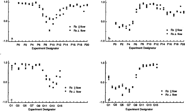
Intermediate solutions X and Y and their standard deviations. a. X values on the P line; b. Y values on the P line; c. X values on the Q.line; d. Y values on the Q.line.

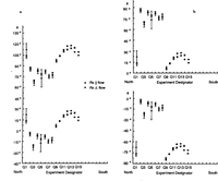
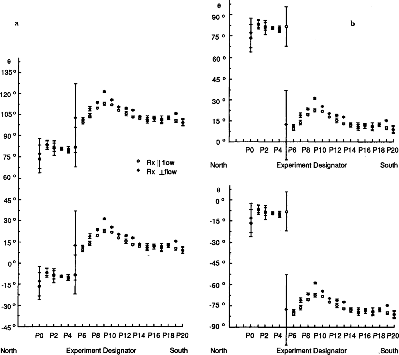
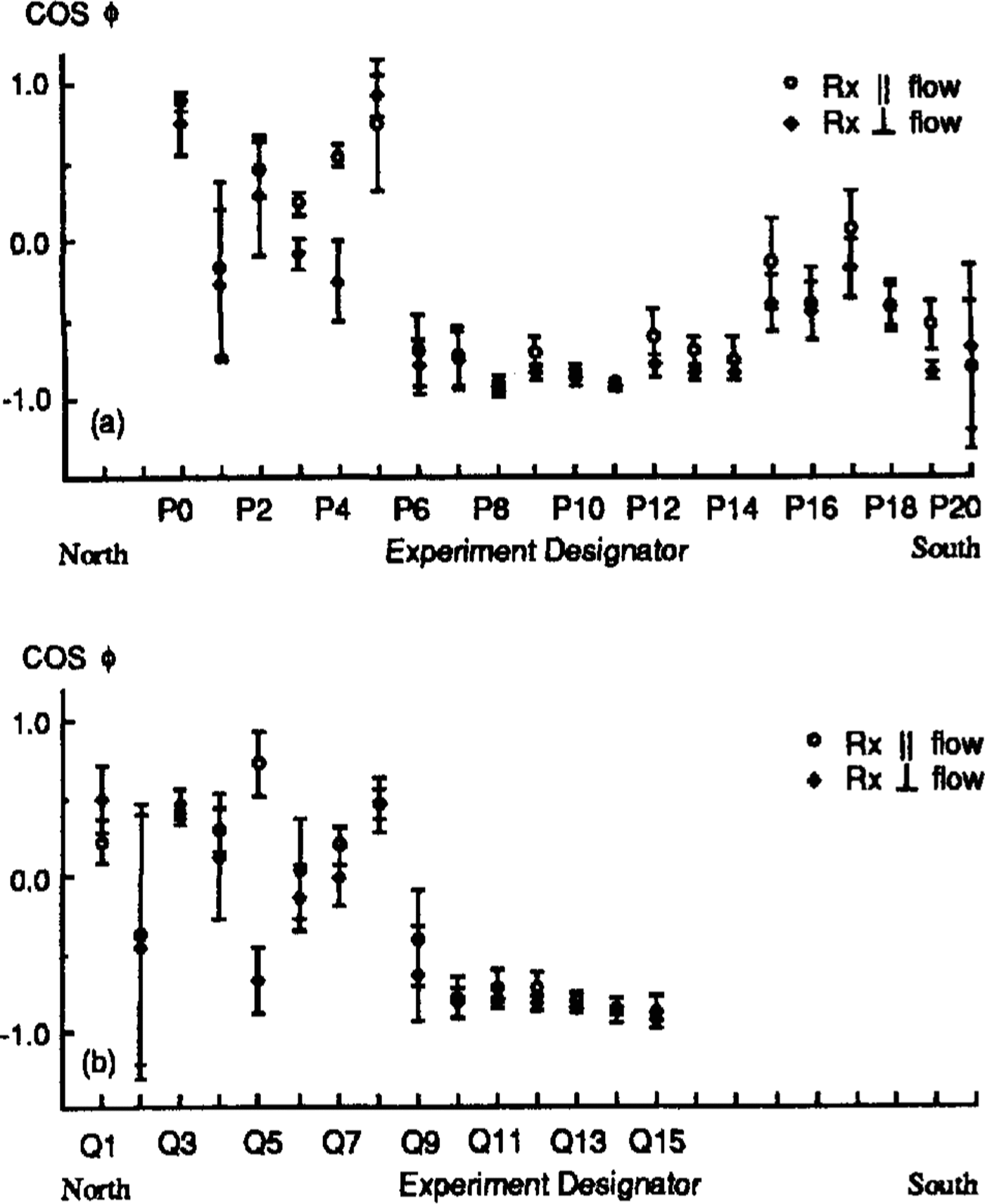
Plots ofθ, the angle in the horizontal between flow and the axis of symmetry, on the P line. Values for the two orientations of the receiving antenna are shown separately. Error bars denote standard deviations. The experiments arespaced 100m apart (see Fig. 1). The left hand and right hand sets of figures each show alternative models; those in (a) arefor the smaller discontinuity at P5; those in (b) are for the larger discontinuity at P5.
Theoretical Model
Uniaxial model
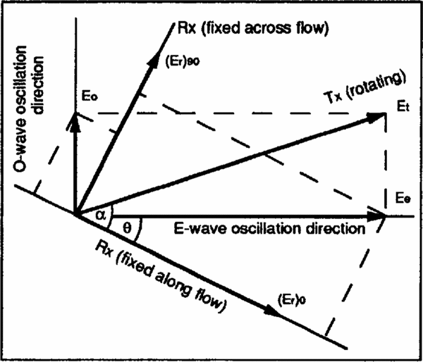
We assume that ice behaves as a uniaxial birefringent medium and consider a radio wave propagating at normal incidence from the ice surface with electric-field amplitude Et . Upon passage through the ice, the wave separates into extraordinary and ordinary waves, which,after reflection at depth h, can be expressed by their electric fields (Figure 2 shows the geometry)

Sketch of a polarization experiment. The(horizontal) snow surface lies in the plane of the diagram and the wave propagates vertically, Rx and Tx denote receiving and transmitting antennas, respectively. The two Rx directions are alternative, not simultaneous, orientations.
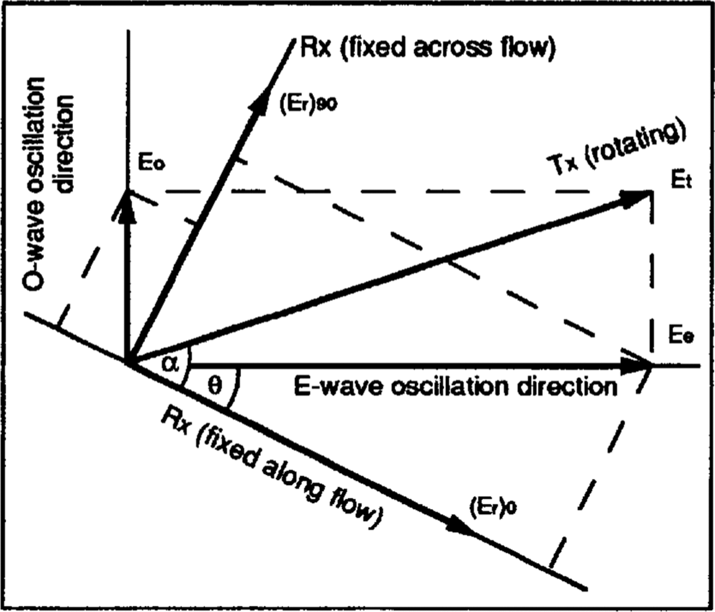
Where ω is the angular frequency, α is the angle between the transmitting antenna and the flow direction,θ is the angle in the horizontal plane between the c-axis orientation and flow,Ve v0 is the extraordinary-wave speed,Ke and Ko are the overall attenuation coefficients of the extraordinary and ordinary waves, respectively, due to absorption,reflection loss and geometrical attenuation, and t is the two-way travel time.
The relative powers received along and across flow,(E r)0and(E r)90,respectively,are then(Reference DoakeDoake, 1981)

and

where
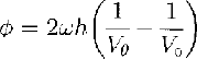
is the phase difference between extraordinary and ordinary waves, and r = Ke/Ko . The unknowns of interest are θandcosϕ;they can be found by least squares from the 24 sets of and(E r)0(or (E r)90) that have been measured in the field. For an isotropic reflector r= 1, and, from Equations (1) and(2)


Where X = cos22θsin22θ cos ϕ and Y = cos2θ sin2θ (1 - cosϕ), whence

and

From Equations (4) and(5), (K o E t)2can be found using the conservation of power
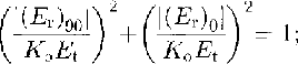
Xand Y can be found by least squares from Equations (4) and(5), then tan 2θ and cos ϕ follow directly from Equations (6) and(7) . Neither θ norϕ is a single-valued function of X and Y For any solution, θ1 , of Equations (6), θ1+π/2 is also a solution. That means that a rotation of the c-axial pattern through 90° in the horizontal plane would not affect the results. Similarly,for any solution 1 ofEquations (7),ϕ1+2nπand(2n - 1)π-ϕ1 are also solutions for any integer n that simply reflects the in determinacy of the total phase shift between the ordinary and extraordinary waves.Note, however, that tan2θ and cos ϕ can be found whatever the wave speeds (so long as they are different).
In the vertical cross-section containing the c axis,called the principal plane, we can diagram the velocity functions (wave speeds as functions of the angle between the c axis and the vertical) (Fig.3). The ordinary wave,with polarization normal to the principal plane, propagates with a speed that is independent of direction, i.e.its velocity function is circular. The velocity function forthe extraordinary wave, which oscillates in the principal plane, is an ellipse.
Sketch of the wave fronts of the ordinary and extraordinary rays in the vertical cross-section containing the c axis (Principal plane). The angles (β and ξare defined in this figure, θin Figure 2. Other quantities are explained in the text.
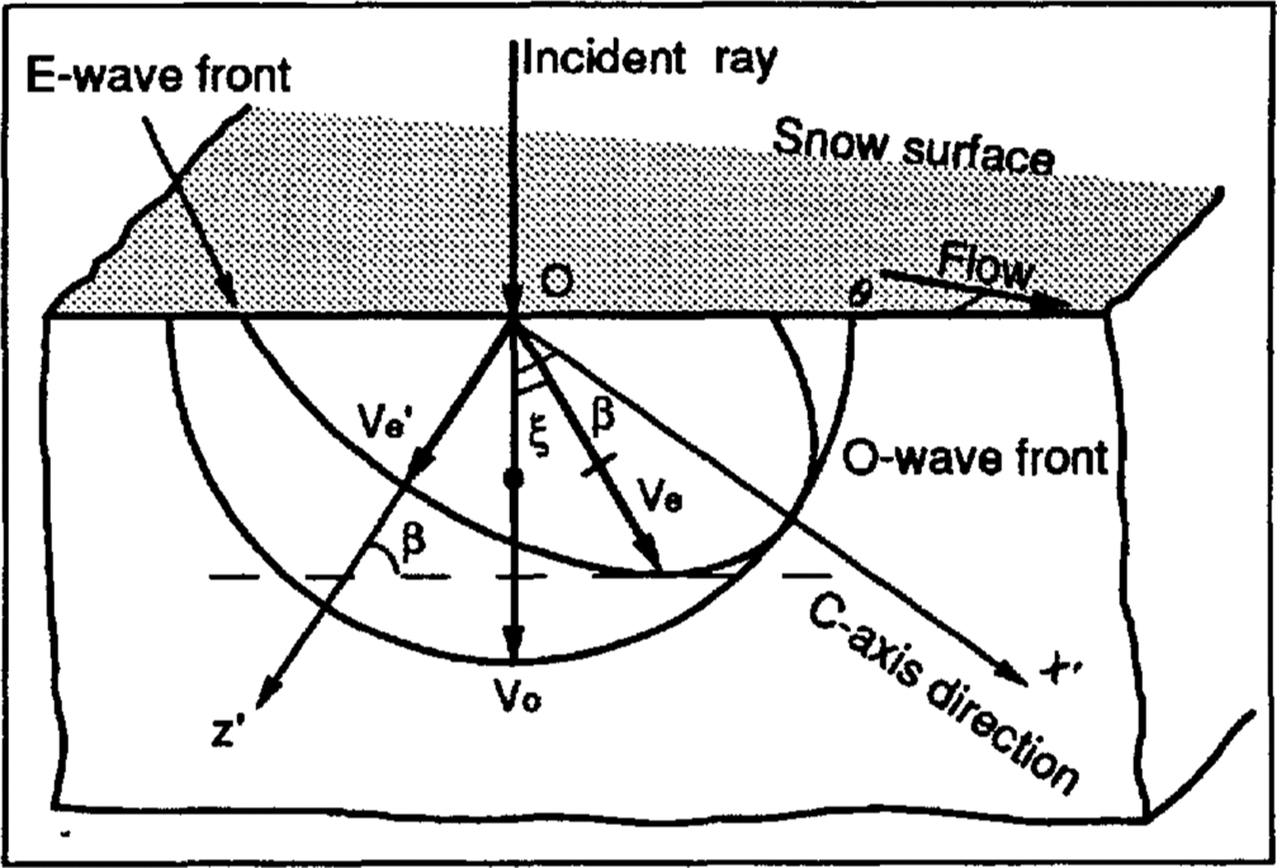
According to Huygen's principle, the extraordinary wave that has a horizontal wave front actually propagatesat a slight angle, ξ to the vertical (unless the c axis is horizontal or vertical). From the geometry in Figure 3,the angle between ordinary and extraordinary rays can be shown to be
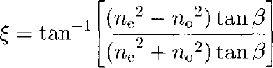
where no= C/Vo and ne = C/Ve ' are the refractive indexes of the ordinary and extraordinary waves, respectively, Ve ' is the minimum of the extraordinary- wave speed for propagation perpendicular to the c axis), C is the speed of light and β is the angle between the vertical and the c axis. The permittivity difference between extraordinary and ordinary waves in ice is less than 2% (Reference Hippel, Knoll, Westphal, Maidique, Iglesias and MykolajewyczVon Hippel and others, 1969; Reference Woodruff and DoakeWoodruff Doake, 1979; Reference Fujita, Mac and MatsuokaFujita and others(1993)), so ξ<0.63°For our purposes, the ordinary and extraordinary waves, therefore, can be considered as propagating in the same direction
The phase difference between the reflected ordinary and extraordinary waves is, from Equation (3),

where f is the frequency. Since Ve ' ≈ Vo the two-way travel time of both waves is approximately t = 2h/Vo , and by Taylor expansion
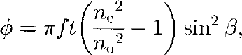
so
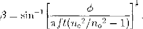
Note that there is more than one solution for the c-axis tilt β, because our technique yields only cos ϕ, not ϕ.
c axes distributed uniformly in a cone
If the c axes are distributed evenly in a cone, the axis ofthe cone becomes the effective c axis, and the extraordinary- wave speed is between Vo , and Ve ' . However,each of the equations for the uniaxial model is still true if one substitutes an effective refractive index for ne . That effective refractive index can be calculated for any assumed cone angle.
c axes distributed randomly in the principal plane
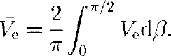
Under some circumstances, the c axes rather than clustering around a single direction tend to be distributed randomly in the principal plane. In this case, the average extraordinary-wave speed,Ve ,is, closely enough (the range of Ve , is so small that averaging slownesses would give a negligibly different result):
Since Vo- Ve '≪ Vo we can approximate the ellipticalvelocity function for the extraordinary wave by

integration then yields

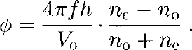
The phase difference between the two waves IS, from Equation (3),
Results
In our field measurements no clear and consistent internal reflections were seen, so only bottom echoes were analyzed. The bottom echoes were about l μs long. We assume a uniform, single layer of ice and an isotropic reflection coefficient.
Figure 4 shows the values of X and Y calculated. from Equation(4) and(5). There are two sets of each for each site, corresponding to the two orientations of the receiving antenna. The error bars depict the standard deviations of the values obtained from the 24 orientations of the transmitting antenna. Note that the standard deviations are all small and that pairs of values are mostly in good agreement.
The corresponding values of θ and cos ϕ are shown in Figures 5-7. We plot cosϕ (Fig. 7) rather than ϕ to avoid multiple values, which we shall consider below. we wishto depict the different possible values of θ, however, so they are shown in Figures 5 and6.
Plots θ, the angle in the horizontal plane between flow and the axis of symmetry, on the Q line. Values.for the two orientations of the receiving antenna are shown separately. Error bars denote standard deviations. The experiments arespaced 100 m apart (see Fig. 1). The left hand and righthand sets figures each show alternative models; those in (a) are for the smaller discontinuity around Q9, those in (b) are for the larger discontinuity around Q9.
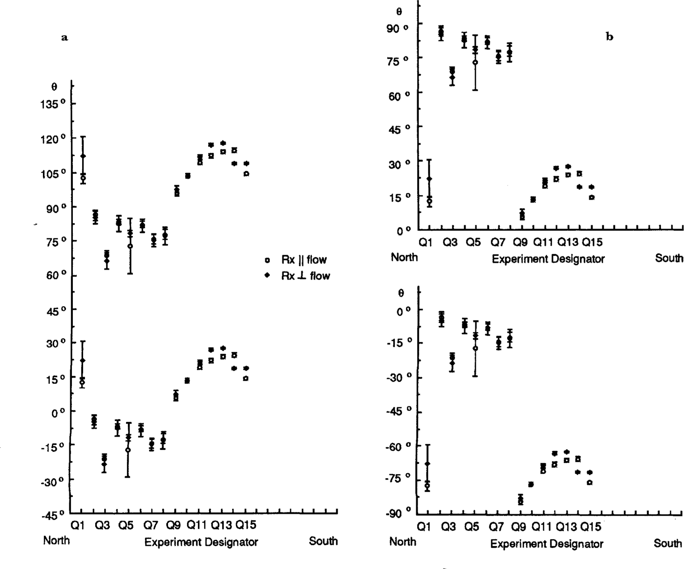
Cosines of the phase differences between ordinary-wave and extraordinary-wave reflections. Values for the two orientations of the receiving antenna are shown .separately. Error bars denote standard deviations. The experiments are spaced 100m apart (seeFig .1). a. P line; b Q line.
Setting the matter of multiple values a side for the moment, we note first that the individual values of θ andcos ϕ are not well determined, despite the small errors inX and Y. That is because θ and cos ϕ become independentof X and Y for particular values (cos ϕ= 1; θ = 0°, 90°);as those values are approached, θ and cos ϕ become increasingly sensitive to small changes in X and Y.
To see this, we consider the standard deviations ofθ and cos ϕ:

and

where m x and m y are the standard deviations of X and Y and EX EY , FX : and FY are the coefficients for error propagation:

and

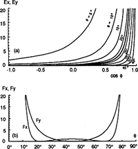
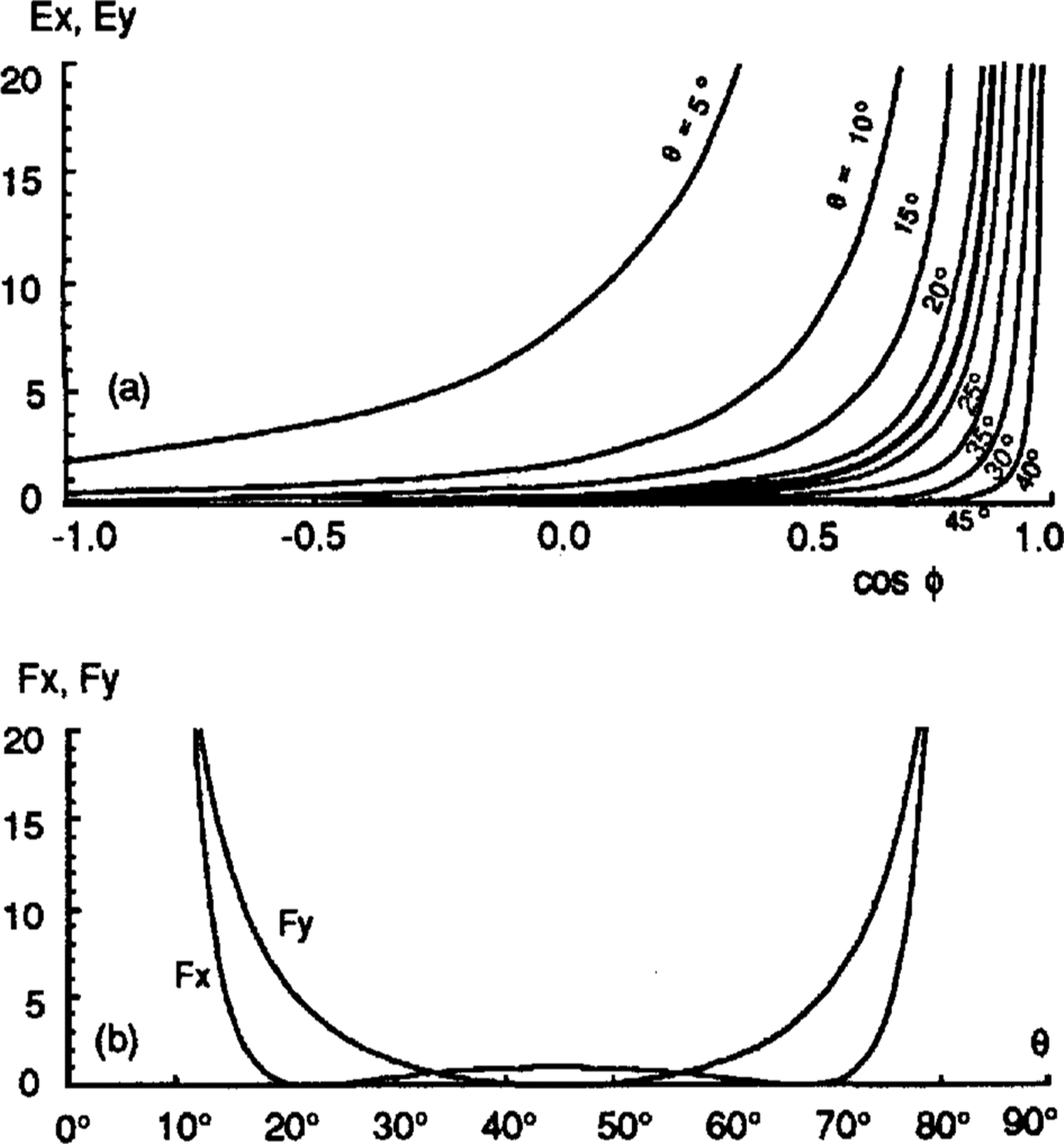
E X, E Y, F X and F Y are plotted in Figure 8 as functions of θand cos ϕ (note that EY is independent of θ and that FX and FY both independent of ϕ.
From Figure 8, we can see why both θ and cos ϕ are more poorly determined in the northern parts of the profiles in Figure 1-7 (P0-P5, Q1-Q8) than in the southern parts -θ is scattered because cos ϕ is near 1 andcosis scattered because θ is near 90°.
The coefficients of error propagation for me, the standard deviation of θ values. Light lines show EX;heavy line shows EY. b. The coefficients of errorpropagation for mcosϕ, the standard deviation cos ∅values
Despite these factors, it is clear that there are abrupt changes in θ between P4 and P6 (Fig. 5) and between Q8 and Q9 (Fig. 6); marked changes in cosϕ also appear in thesame places (Fig. 7). These step changes stem from discontinuities in Y (Fig. 4). The amount of change in θ is not certain, however, because of its double valued ness. Thesmaller possible change in θ is about 30°, with values centered around either 0° or 90° (Figs 5a and6a), but a larger step of about 60° cannot be ruled out (Figs 5b and 6b).
To us, the large and abrupt changes argue against anisotropic reflection as the principal cause of depolarization.Not only is there no known model [or an anisotropic reflection coefficient that would mimic such phase shifts, it is hard to see how an actively deforming bed, the anisotropic characteristics of which (if any)would have to be tied to its movement along the flow direction, could show such a rapid lateral change where there is no discontinuity in flow. Anisotropic absorption could conceivably cause the observed effect but, since it has never been reported in ice, where as anisotropy in the permittivity of an ice crystal is a known phenomenon, we will proceed on the assumption that the observed depolarization arises from the latter.
We first apply the uniaxial model. To calculate the dip of the effective c axis, β (Equation (8)), we adopt the permittivity values of Reference Fujita, Mac and MatsuokaFujita and others(1993)): = 3.189 ± 0.006 and
 = 3.152 ± 0.003; then
 and
 There are seven options for β, ranging from 10° to 80°, because only cos ϕ is known; ϕ could theoretically have a value as large as 7.5πfor horizontal caxes, corresponding to β = 90°
. In reality, of course, the c axes are never perfectly aligned. A conical distribution ofc axes would yield an effective anisotropy less than the single-crystal value by an amount that would depend onthe details of the distribution. The effect of that would bet o reduce the maximum possible phase difference,probably by a substantial amount, and thus to eliminatethe smallest values ofθ(nearest-to-vertical orientations)from the allowable set. Another factor that would tend to reduce the allowable set further is that the whole ice sheetis probably not characterized by the same anisotropy;certainly, it cannot be expected to extend right to the surface (Reference BlankenshipBlankenship, 1989). Reducing the fraction of the ice sheet to which the single-crystal model appliesincreases the required effect from that fraction.
If a conical model applies, therefore, the axis of symmetry is not near vertical. It is likely for theoretical reasons that the axis is along one of the principal stresses(Reference AlleyAlley, 1992) and the absence of strong shear stress at thebed (Reference Kamb and EngelhardtKamb and Engelhardt, 1991) means that the principal stress axes arc probably nearly vertical and horizontal. It follows, then, that the axis of symmetry of the ice fabric is probably nearly horizontal.
If we take as an alternative model, c axes distributed randomly in the vertical plane normal to flow, as found from seismic work near UpB Camp (Reference BlankenshipBlankenship, 1989),the phase difference between the two waves over the whole ice thickness, according to Equation (9), is 3.97π.This would also be reduced by a spreading of the c-axial directions out of the principal plane and by the applicability of the model to less than the entire ice column. Nevertheless, there is still ample phase difference available in the alternative model to accommodate any observed value of cos ∅ This model also implies a horizontal axis of symmetry.
Whatever the ambiguity in the specific c-axis model,the results show strikingly different characteristics of theice on opposite sides of a boundary that runs parallel to flow (dotted line in Figure 1). This contrast supports the concept of two distinct blocks of ice with different fabrics,hence different stress/strain histories.
We can use the seismic measurements (Reference BlankenshipBlankenship,1989) to help choose between models. Projecting these is mic site directly upflow would put it 23 km to the south of profiles P and Q It is likely, then, that the c axes on the southern parts of the profiles also lie in a transverse vertical plane, as they do at the seismic site. This would mean that θ≈ 90° , which would in turn argue against the validity of the lower model in Figures 5aand6a and the upper model in Figures 5band6b
Another clue comes from strain measurements. Shear strains in the horizontal plane should be sensitive to the orientation of the c-axes in the horizontal plane, since the shear stress should change in some smooth way across the ice stream. Thus, it seems likely that a shift in c-axis orientation from nearly normal to flow to nearly along flow across the boundary between the northern and southern zones in the profiles would produce anomalous shear strains. However, the recent survey by Reference Hulbe and WhillansHulbe and Whillans (1994) does not show any abnormal shear strains in this location, so we conclude that the models of Figures 5band6b are less likely than those ofFigures 5aand6a We are left, then, with the upper models in Figures 5aand6a as the ones we believe are closest to being correct.
Conclusions
Radar-polarization studies strongly indicate the existence,at a location on Ice Stream E, of an abrupt change in crystalline fabric across a distance of only 100 or 200 m perpendicular to flow. From several models that fit the data, we prefer the one that is consistent with local strain data and with fabrics estimated from seismic measurements 10 km downstream. In this model, theaxis of symmetry of the fabric is rotated by 30° across the boundary, from + 15° to 15° relative the directiontransverse to flow, as if the two parts of the profile lay onblocks of ice with different stress/strain histories. It iseven possible that profile Q spans a block - note thatthe orientation at the most northerly site, Q1, is“normal”, i.e. the same as for the southern (right-hand)section. The occurrence of exotic blocks withinice steams has been suggested by several authors inrelation to ice rafts (Reference Bindschadler, Stephenson, MacAyeal and ShabtaieBinds chadler and others, 1987),discontinuity in mass flux (Reference BlankenshipShabtaie and others, 1988)and irregular features within the ice stream (Reference WhillansWhillans,1987) .
Acknowledgements
The authors would like to thank T. S. Clarke and A. N.Novick tor their help with the field work. This paper wassupported by U.S. National Science Foundation grantDPP-90-18530. This is contribution No. 543 of the Geophysicaland Polar Research Center, University ofWisconsin-Madison.