Implications
Results of the present study show that the inductive causation algorithm, a technique for estimating how variables are causally related, provided clues of phenotypic causal networks among reproductive traits including calf size. By fitting the structural equation model to the structures, useful information such as the magnitude of the causal effects between traits could be obtained. Applying these techniques to reproductive and calf-size traits can provide estimates of the calf body size as well as the associated increase in risks of calving difficulty (dystocia) due to an extended gestation period.
Introduction
Reproduction-related traits have been of increasing interest to Japanese beef cattle industry, as there is an urgent need to boost the cow population in Japan. Calving difficulty (CD), namely, dystocia is a cause of mortality in cows and calves; it increases the postpartum interval and decreases the conception rate. It leads to not only increased labor and veterinary costs, but also loss of production and impaired reproductive performance of cows.
Revealing the associations between CD and potentially related traits, such as gestation length (GL) and birth weight (BWT), is crucial for improving the reproductive performance of cows in a breeding system. A number of studies have reported correlations among the traits related to calf production (Hansen et al., Reference Hansen, Lund, Pedersen and Christensen2004; Ibi et al., Reference Ibi, Kahi and Hirooka2008; Mujibi and Crews, Reference Mujibi and Crews2009). In addition, recursive causal relationships between some of the reproductive traits have been inferred in a few reports (Lopez de Maturana et al., Reference Lopez de Maturana, Wu, Gianola, Weigel and Rosa2009; Mokhtari et al., Reference Mokhtari, Moradi Shahrbabak, Nejati Javaremi and Rosa2016), usually by fitting a structural equation model that estimates the magnitude of causal effects between traits (Wright, Reference Wright1921; Haavelmo, Reference Haavelmo1943). Ever since Gianola and Sorensen (Reference Gianola and Sorensen2004) proposed adaptations of structural equation model in the context of quantitative genetics and mixed effect models, a number of studies have applied the structural equation model in a breeding context, mainly for reproductive (Lopez de Maturana et al., Reference Lopez de Maturana, Wu, Gianola, Weigel and Rosa2009; Mokhtari et al., Reference Mokhtari, Moradi Shahrbabak, Nejati Javaremi and Rosa2016) or health traits.
However, these studies assumed that the causal structures were known a priori. Valente et al. (Reference Valente, Rosa, Gianola, Wu and Weigel2010) adapted the inductive causation (IC) algorithm (Verma and Pearl, Reference Verma and Pearl1990; Pearl, Reference Pearl2000), which allows searching for how the variables are causally related, to a mixed models context. The authors also showed that applying this method to the posterior distribution of the residual variance and covariance matrix of a standard multiple-trait model recovered the expected network in simulated data. The causal structure inferred using the IC algorithm could then be applied to define the structural equation model.
To the best of our knowledge, only a few studies fitted the structural equation model to a causal structure inferred using the IC algorithm, for example, those involving European quail (Valente et al., Reference Valente, Rosa, Silva, Teixeira and Torres2011), bovine milk fatty acids (Bouwman et al., Reference Bouwman, Valente, Janss, Bovenhuis and Rosa2014) and meat quality traits in Japanese Black cattle (Inoue et al., Reference Inoue, Valente, Shoji, Honda, Oyama and Rosa2016). Therefore, the objective of this study was to search for phenotypic causal structures and to infer the relationships among GL, CD and birth body measurements of calves in Japanese Black cattle. In addition, we compared the causal effects from fitting the structural equation model with the causal structures based on the results from the IC algorithm and those based on biological prior knowledge.
Material and methods
Animal Care and Use Committee approval was not needed for this study because it involved the use of preexisting data from the database of the National Livestock Breeding Center (NLBC), Japan.
Animals and data
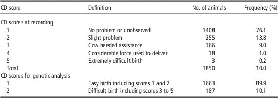
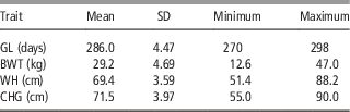
The GL of Japanese Black heifers and their CD for the primiparity (first calving), as well as the BWT, withers height (WH) and chest girth (CHG) of their full blood calves were obtained from the four breeding stations of the NLBC. Calving difficulty was scored on a 1 to 5 scale by the technicians of the NLBC, where 1=no problem or unobserved, 2=slight problem, 3=cow needed assistance, 4=considerable force used to deliver calf and 5=extremely difficult birth. The body measurements of the calves were measured within 3 days of their birth. The data that satisfies the following conditions were adopted: the calving age of the heifers ranged from 21 to 37 months, the GL ranged from 270 to 300 days, calves were born with artificial insemination and single births. Finally, 1850 records of these traits were used in the present study. The distribution of CD and the descriptive statistics for GL, BWT, WH and CHG are shown in Tables 1 and 2, respectively.
Distribution of calving difficulty (CD)

Descriptive statistics for gestation length (GL), birth weight (BWT), withers height (WH) and chest girth (CHG) used in this study

The multiple-trait model analysis
For the purpose of genetic analysis, CD scores were divided into two categories: 1=easy birth (included scores of 1 and 2) and 2=difficult birth (included scores of 3 to 5). Therefore, the CD was assumed to be binary data, which should follow a liability scale. The observations for the diseases were denoted as follows:
 $$y_{{{\rm CD}}} \, {\equals}\, \left\{ {\matrix{ {0 \,{\rm\quad if}\,U_{{{\rm CD}}} \leq T_{{{\rm CD}}} } \cr {1 \,{\rm \quad if}\,U_{{{\rm CD}}} \,\gt\,T_{{{\rm CD}}} } \cr } } \right.$$
where U CD and T CD denote a liability and a threshold for CD, respectively. To analyze the correlations among CD, GL and the other body measurements, a three-trait linear-threshold sire-maternal grand sire (MGS) model was fitted to the triplets including the underlying liability for CD, the linear observation of GL and BWT, WH or CHG. The three-trait model was also fitted to BWT, WH and CHG to clarify the associations between the calf body measurements. The model, which was used for estimating the (co)variance components, can be written in matrix notation as follows:
 $${\bf y}\,\left( {\bf U} \right){\bf \, {\equals}\, X}{\mib \bbeta } {\bf {\plus}Wh{\plus}Z}_{{\bf 1}} {\bf s{\plus}Z}_{{\bf 2}} {\bf mgs{\plus}e}$$
with the joint distribution of vectors h, u=[s mgs]', and e as:
 $$\left[ {\matrix{ {\bf h} \cr {\bf u} \cr {\bf e} \cr } } \right]{\bf \,\sim\,N}\left\{ {\left[ {\matrix{ {\bf 0} \cr {\bf 0} \cr {\bf 0} \cr } } \right]{\bf ,}\left[ {\matrix{ {{\bf H}_{{\bf 0}} {\bf ⊗I}} & {\bf 0} & {\bf 0} \cr {\bf 0} & {{\bf G}_{{\bf 0}} {\bf ⊗ A}} & {\bf 0} \cr {\bf 0} & {\bf 0} & {{\bf R}_{{\bf 0}} {\bf ⊗ I}} \cr } } \right]} \right\}$$
where y is a vector of observed traits (GL, BWT, WH and CHG), U the vector of unobserved liabilities of CD, β the vector of fixed effects, which includes the sex of calves (two levels: male and female) and month of calving (12 levels), h the vector of contemporary group effects, which includes herd-year at calving (42 levels), s and mgs the vectors of random sire and MGS effects, e the vector of random residual effects and X, W, Z 1 and Z 2 are known incidence matrices. H 0 is the diagonal variance matrix for contemporary group effect, G 0 the sire-MGS (co)variance matrix, A the additive genetic relationship matrix, R 0 the residual (co)variance matrix and I the identity matrix with suitable dimensions. To identify the parameters, the threshold and the residual variances for CD were arbitrarily set to 0 and 1, respectively.
The program THRGIBBS1F90 (Tsuruta and Misztal, Reference Tsuruta and Misztal2006) was used for obtaining posterior distributions of genetic and residual (co)variances. The (co)variance components were determined based on a generated Gibbs sampling chain of 100 000 samples after 100 000 samples as burn-in, based on a visual inspection of trace plots and posterior distributions. The results of Geweke’s diagnostic and effective sample size from the program POSTGIBBSF90 (Misztal et al., Reference Misztal, Tsuruta, Strabel, Auvray, Druet and Lee2002) were also used to assess convergence.
Sire variance,
 $$(\sigma _{{\rm s}}^{2} )$$
MGS variance
 $$(\sigma ^{2} _{{{\rm mgs}}} )$$
and sire-MGS covariance
 $\left( {\sigma _{{{\rm s,mgs}}} } \right)$
were converted to direct
 $$(\sigma _{{\rm D}}^{2}) $$
, maternal
 $$(\sigma _{{\rm M}}^{2} )$$
genetic variances and their covariance
 $$(\sigma _{{{\rm D,M}}} )$$
as follows (Willham, Reference Willham1972):
 $$\left[ {\matrix{ {\sigma _{{\rm D}}^{2} } \cr {\sigma _{{{\rm D,M}}} } \cr {\sigma _{{\rm M}}^{2} } \cr } } \right]\, {\equals}\, \left[ {\matrix{ 4 & 0 & 0 \cr {{\minus}2} & 4 & 0 \cr 1 & {{\minus}4} & 4 \cr } } \right]\left[ {\matrix{ {\sigma _{{\rm s}}^{2} } \cr {\sigma _{{{\rm s,mgs}}} } \cr {\sigma _{{{\rm mgs}}}^{2} } \cr } } \right]$$
Phenotypic variance
 $$(\sigma _{{\rm p}}^{2} )$$
and the heritabilities of direct
 $$(h_{{\rm D}}^{2} )$$
and maternal
 $$(h_{{\rm M}}^{2} )$$
genetic effects were calculated as:
 $$\sigma _{{\rm p}}^{2} \, {\equals}\, \sigma _{{{\rm hy}}}^{2} {\plus}\sigma _{{\rm s}}^{2} {\plus}\sigma _{{{\rm s,mgs}}} {\plus}\sigma _{{{\rm mgs}}}^{2} {\plus}\sigma _{{\rm e}}^{2} $$
 $$h_{{\rm D}}^{2} \, {\equals}\, {{\sigma _{{\rm D}}^{2} } \over {\sigma _{{\rm p}}^{2} }}, \ h_{{\rm M}}^{2} \, {\equals}\, {{\sigma _{{\rm M}}^{2} } \over {\sigma _{{\rm p}}^{2} }}$$
where
 $$\sigma _{{{\rm hy}}}^{2} $$
is the variance of contemporary group.
The inductive causation algorithm
The IC algorithm was applied to the residual (co)variances obtained from the multiple-trait model analysis. This algorithm could be potentially applied on the genetic (co)variance matrix as well. However, there may be some controversy about that, especially in regards to causal inference. A causal interpretation for the inferred structure would be indicating that the breeding value of an individual for a specific trait would be affecting its breeding value for another trait. This would be conceptually completely against what is nowadays accepted in terms of sources of relationships between breeding values for different traits, that is pleiotropism and linkage disequilibrium between genes affecting different traits. In view of this, we used the residual variance components to infer a causal structure among phenotypes as proposed by Valente et al. (Reference Valente, Rosa, Gianola, Wu and Weigel2010). The residual variance components were considered as information from the joint distribution of the phenotypic traits, conditional on genetic effects (Valente et al., Reference Valente, Rosa, Gianola, Wu and Weigel2010). However, the multiple-trait sire-MGS model was fitted in the multiple-trait model analysis and therefore, maternal genetic effect could not be removed completely from the residual variance components. Thus, applying the IC algorithm to the variances from the sire-MGS model in this study should be considered as a preliminary trial for detecting causal relationships between the traits.
The algorithm makes a series of statistical decisions based on partial correlations between traits and consists of three steps (Pearl, Reference Pearl2000). The steps have been described in detail by Inoue et al. (Reference Inoue, Valente, Shoji, Honda, Oyama and Rosa2016), and hence, are briefly described here. In the first step, two traits are connected with an undirected link (e.g. y1−y2) under the conditions of statistical decisions based on partial correlations (Step 1). In the second step, undirected links in a triplet obtained in Step 1 (e.g. y1−y2−y3) change into directed ones toward the common adjacent trait (i.e. y1→y2←y3), forming a so-called ‘unshielded collider,’ using the statistical decisions (Step 2). Finally, with the graph obtained in Step 2, as many undirected links as possible are oriented without creating a new unshielded collider or cycle (Step 3).
Statistical decisions regarding whether to declare partial correlations as null or not were based on highest posterior density (HPD) intervals. If the interval contained the value zero, the correlation was declared as null. Outputs might differ according to the probability content used for the decision. We applied different HPD intervals (80%, 85%, 90% and 95%) to evaluate the structure sensitivity. The analysis was carried out using the program ICPS (Valente and Rosa, Reference Valente and Rosa2013) written in R (R Development Core Team, 2009).
The structural equation model analysis
The structural equation model was fitted to the causal network inferred by the IC algorithm application. The structural equation model can be described as:
 $${\bf y}\left( {\bf U} \right){\bf \, {\equals}\, }\left( {{\bf \bLambda ⊗ I}} \right){\bf y{\plus}X}{\mib{\bbeta }} ^{{\bf {\asterisk}}} {\bf {\plus}Wh}^{{\bf {\asterisk}}} {\bf {\plus}Z}_{{\bf 1}} {\bf s}^{{\bf {\asterisk}}} {\bf {\plus}Z}_{{\bf 2}} {\bf mgs}^{{\bf {\asterisk}}} {\bf {\plus} e}^{{\bf {\asterisk}}} $$
with the joint distribution of vectors h *, u * =[s * mgs *], and e * as:
 $$\left[ {\matrix{ {{\bf h}^{{\bf {\asterisk}}} } \cr {{\bf u}^{{\bf {\asterisk}}} } \cr {{\bf e}^{{\bf {\asterisk}}} } \cr } } \right]{\bf \,\sim\,N}\left\{ {\left[ {\matrix{ {\bf 0} \cr {\bf 0} \cr {\bf 0} \cr } } \right]{\bf ,}\left[ {\matrix{ {{\bf H}_{{\bf 0}}^{{\bf {\asterisk}}} {\bf ⊗ I}} & {\bf 0} & {\bf 0} \cr {\bf 0} & {{\bf G}_{{\bf 0}}^{{\bf {\asterisk}}} {\bf ⊗ A}} & {\bf 0} \cr {\bf 0} & {\bf 0} & {{\bf \Psi }_{{\bf 0}} {\bf ⊗ I}} \cr } } \right]} \right\}$$
where y, U, β
*, h
*, s
*, mgs
*, e
*, X, W, Z
1
, Z
2
,
 ${\bf{H}} _{{\bf{0}} }^{{\bf{{\asterisk}}} } $
, A and I have similar meanings for the multiple-trait model as described above, but these vectors represent systematic and random effects that affect each trait directly, that is, effects that are not mediated by other phenotypic traits (Gianola and Sorensen, Reference Gianola and Sorensen2004; Rosa et al., Reference Rosa, Valente, De Los Campos, Wu, Gianola and Silva2011; Valente et al., Reference Valente, Rosa, de los Campos, Gianola and Silva2013). In addition, Λ is a t×t (where t is the number of traits) matrix with zeroes on the diagonal and with structural coefficients (linear effects between pairs of traits) or zeroes on the off-diagonals,
 $${\rm \bf G}_{\bf 0}^{{\bf \asterisk}} $$
is an additive genetic (co)variance matrix (i.e. it describes variances and covariances of direct genetic effects) of the structural equation model and
 $$\bf \Psi _{0} $$
is a diagonal matrix with residual variances of the structural equation model. The residual covariances between the traits in the structural equation model were assumed to be zero. This parametric restriction confers identifiability to the structural coefficients in the likelihood function.
The program used for the standard multiple-trait model (THRGIBBS1F90, Tsuruta and Misztal, Reference Tsuruta and Misztal2006) was also used for obtaining posterior distributions of the structural equation model parameters. Causal parents (e.g. y1 is the causal parent of y2 in y1→y2) of a given trait were included as covariates in the equations assigned to that trait, and a diagonal residual covariance matrix was imposed. Conditions for generating Gibbs sampling chain and the convergence criteria were the same as the multiple-trait model analysis. Therefore, the posterior probabilities of the structural equation model unknowns were characterized based on the remaining 100 000 samples.
Posterior analysis of structural coefficients
As described above, CD was assumed to be under a liability scale. If a causal structure that was detected by the IC algorithm included a structure such as GL on CD (λ CD,GL) or BWT on CD (λ CD,BWT), the rates of change for the structural coefficients would be expressed in liability scale. Here, λ i,j denotes a structural coefficient from the jth trait to the ith trait. Therefore, the coefficients were transformed to the observable scale (OS) using the method by Lopez de Maturana et al. (Reference Lopez de Maturana, Wu, Gianola, Weigel and Rosa2009). The method fitted for λ CD,BWT is described below as an example and this can also fit for other structural coefficients on CD.
If λ CD,BWT is positive, an increase in BWT by 1 kg will increase liability to CD by λ CD,BWT units per kg. This indicates that the probability of CD increases and the threshold T CD ‘moves to the left.’ If λ CD,BWT is negative, the liability to CD decreases, the probability of CD also decreases and the threshold T CD ‘moves to the right.’ Therefore, the difference (D) between the probability of having CD before and after a change of 1 kg in BWT can be calculated as:
 $${\rm D}\, {\equals}\, \hat{\lambda }_{{{\rm CD},{\rm BWT}}} {\rm \varphi }\left( {{{\hat{T }__{{{\rm CD}}} {\minus}\hat{\mu }_{{{\rm CD}}} } \over {\hat{\sigma }_{{{\rm e}_{{{\rm CD}}} }} }}} \right)$$
where φ is the probability density function, and
 $$ \hat{\mu }_{{{\rm CD}}} $$
and
 $$\hat{\sigma }_{{{\rm e}_{{{\rm CD}}} }} $$
the mean and residual standard deviation of the liability to CD, respectively. The value on the underlying scale corresponding to the mean on the OS is (89.9%, Table 1) is 1.2759. As mentioned, the residual variance is equal to 1.
Results and discussion
Phenotype measurements
Distribution of calving ease is shown in Table 1. The percentage of difficult birth (scored 4 and 5) was approximately 10%. Carnier et al. (Reference Carnier, Albera, Dal Zotto, Groen, Bona and Bittante2000) reported that the percentage of scores >3 in the five categories of CD was 28.4% at primiparity in Piedmontese cattle and this was higher than the level of CD in our study. However, the mean CD score in the present study was 1.37 (data not shown), which is higher than that in Limousin (1.20, Matilainen et al., Reference Matilainen, Mrode, Stranden, Thompson and Mantysaari2009) and in the same Japanese Black breed (1.069, Uchida et al., Reference Uchida, Kobayashi, Inoue, Suzuki and Oikawa2002), although the latter was the average of three score categories.
Means of GL, BWT, WH and CHG after editing the data were 286.0±4.72 (days), 29.2±4.80 (kg), 69.4±3.59 (cm) and 71.5±3.97 (cm), respectively (Table 2). In the relatively recent reports of GL in Japanese Black cattle in Japan, means±SD of GL were 287.5±4.8 days (Uchida et al., Reference Uchida, Kobayashi, Inoue, Suzuki and Oikawa2002) and 286.51±5.78 (Ibi et al., Reference Ibi, Kahi and Hirooka2008). Their data were collected from across the nation (Uchida et al., Reference Uchida, Kobayashi, Inoue, Suzuki and Oikawa2002) and from 15 prefectures (Ibi et al., Reference Ibi, Kahi and Hirooka2008) in Japan. The mean and SD of GL in the present study were similar to those in the same breed but also to another beef cattle breed, Chalolais (Mujibi and Crews, Reference Mujibi and Crews2009). Ibi et al. (Reference Ibi, Kahi and Hirooka2008) also reported means (±SD) of 27.5 (±4.3) kg for BWT, which was similar to our result. Japanese Black cattle, which is one of the Wagyu breeds, is known to be smaller than the European breeds. The means of BWT in Japanese Black cattle (Ibi et al., Reference Ibi, Kahi and Hirooka2008 and in our study) were lower than those in Chalolais (46.54 kg, Mujibi and Crews, Reference Mujibi and Crews2009) and Limousin (37.29 kg, Matilainen et al., Reference Matilainen, Mrode, Stranden, Thompson and Mantysaari2009). Although BWT in Japanese Black was lower than that in European breeds, CD was more serious in Japanese Black, as described above.
The multiple-trait model analysis
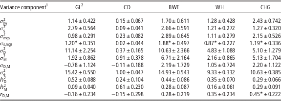
Posterior means and posterior standard deviations (PSD) of the variance components within each trait from the multiple-trait model analysis are shown in Table 3. The variance components for GL and CD were averaged from three analyses, while those for BWT, WH and CHG were from each analysis including GL and CD. The heritability of direct genetic effect in GL (0.52) was higher than that of the maternal one (0.09). This could explain that GL is more affected by sires’ genetic effect on their calves, such as size of calves, than dams’ effect, such as uterine environment. Similarly, the direct heritability for BWT (0.44) and WH (0.35) was higher than the maternal one for BWT (0.28) and WH (0.16). In contrast, the direct heritability for CD (0.24) was lower than the maternal one (0.61). Pelvic size and shape of dam (heifer) could have more influence on CD than the size of calf. The same heritability estimates of direct (0.29) and maternal (0.29) genetic effects were found in CHG, and the genetic correlation between them was significantly (P<0.05) positive (0.45±0.22). This might indicate that CHG is also affected by maternal body and pelvic size.
Posterior means±posterior standard deviations of the variance components within the traits for the multiple-trait model

GL=gestation length; CD=calving difficulty; BWT=birth weight; WH=withers height; CHG=chest girth.
1
 $$\sigma _{{{\rm hy}}}^{2} $$
=contemporary group variance;
 $$\sigma _{{\rm s}}^{2} $$
=sire genetic variance;
 $$\sigma _{{{\rm mgs}}}^{2} $$
=maternal grand sire (MGS) genetic variance;
 $$\sigma _{{{\rm s,mgs}}} $$
=covariance between sire and MGS genetic effects;
 $$\sigma _{{\rm D}}^{2} $$
=direct genetic variance;
 $$\sigma _{{\rm M}}^{2} $$
=maternal genetic variance;
 $$\sigma _{{{\rm D,M}}} $$
=covariance between direct and maternal genetic effects;
 $$\sigma _{{\rm e}}^{2} $$
=residual variance;
 $$h_{{\rm D}}^{2} $$
=direct heritability;
 $$h_{{\rm M}}^{2} $$
=maternal heritability;
 $$r_{{{\rm D,M}}} $$
=genetic correlation between direct and maternal effect.
2 Variance components for GL and CD were averaged from three triplet analyses, which triplets included CD, GL and BWT, WH or CHG; and those for BWT, WH and CHG were from each triplet analysis that included GL and CD.
*95% highest posterior density region does not include 0.
There are many studies that estimate the genetic parameter for CD, GL and BWT; however, to our knowledge, there are no published reports on genetic parameters for CD, WH and CHG at birth in Japanese Black cattle. In addition, CD has been analyzed with two approaches: considered as a trait of the dam or a trait of the calf, as two types of traits: continues trait or categorical (threshold) trait, and using two models: animal model or sire-MGS model. Reported direct and maternal heritabilities from the same condition analysis as this study (considered as a categorical calf trait and with sire-MGS model) ranged from 0.09 to 0.17 and from 0.05 to 0.12, respectively, in Holstein (Steinbock et al., Reference Steinbock, Nasholm, Berglund, Johansson and Philipsson2003; Wiggans et al., Reference Wiggans, Misztal and Van Tassell2003; Hansen et al., Reference Hansen, Lund, Pedersen and Christensen2004; Lopez de Maturana et al., Reference Lopez de Maturana, Wu, Gianola, Weigel and Rosa2009). On the other hand, some studies using beef cattle breed reported moderate direct heritabilities in Italian Piemontese (0.236 to 0.259, Kizilkaya et al., Reference Kizilkaya, Banks, Carnier, Albera, Bittante and Tempelman2002), Angus (0.28), Charolais (0.33) and Simmental (0.21, Trus and Wilton, Reference Trus and Wilton1988), although there were a few differences on the analysis such as fitted models. The estimate of the direct one in the present study (0.24±0.10) was within the range of their estimates. However, the maternal one (0.61±0.23) was higher than those in the previous studies, even though Trus and Wilton (Reference Trus and Wilton1988) reported some moderate maternal ones (around 0.25). This could be due to smaller data size in our study, because the PSD of the maternal heritability was large (0.23).
Genetic parameters for GL have also been estimated with two approaches: considered as a dam trait or as a calf trait. Ibi et al. (Reference Ibi, Kahi and Hirooka2008) estimated the heritability of direct (0.53) and maternal (0.14) genetic effect for GL, which was considered as a calf trait in Japanese Black cattle. The estimates were similar to the results of our study. Mujibi and Crews (Reference Mujibi and Crews2009) reported slightly higher heritabilities of the direct (0.62) and maternal (0.10) effect for GL. These two authors also reported the heritabilities of the direct and maternal effect for BWT, which were 0.31 and 0.06, respectively, as per Ibi et al. (Reference Ibi, Kahi and Hirooka2008), and 0.46 and 0.14, respectively, according to Mujibi and Crews (Reference Mujibi and Crews2009). The estimates in the present study were similar to those reported by these authors. On the other hand, slightly lower estimates for the direct and maternal heritabilities of GL (0.39 to 0.43 and 0.07 to 0.08, respectively) were reported in Holstein (Hansen et al., Reference Hansen, Lund, Pedersen and Christensen2004; Lopez de Maturana et al., Reference Lopez de Maturana, Wu, Gianola, Weigel and Rosa2009).
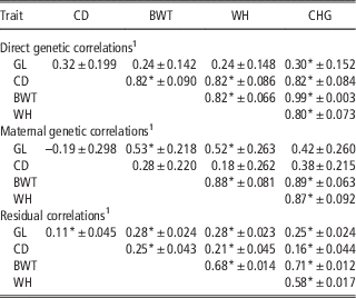
The direct genetic, maternal genetic and residual correlations and their PSD, obtained from the multiple-trait model, are presented in Table 4. The correlations between GL and CD were averaged from three analyses. Between GL and CD, weak positive and negative correlations were found in the direct (0.32) and maternal (−0.19) genetic ones, whereas the correlations were not significantly different from zero. Residual correlation between them was also weak (0.11), but significantly different from zero (P<0.05). The direct genetic correlation between GL and CD in our study was within the range of estimates (0.13 to 0.38), as reported by Hansen et al. (Reference Hansen, Lund, Pedersen and Christensen2004) and Lopez de Maturana et al. (Reference Lopez de Maturana, Wu, Gianola, Weigel and Rosa2009), although the estimate in the present study was not significantly different from zero. In contrast, the maternal one in our study was negative and differed from the positive estimates in the two previous studies (0.12 to 0.23). The 95% HPD region of the estimate in our study included zero and the PSD of the estimate was large (0.298). However, there have been no other reports on genetic correlation between GL and CD in the Japanese Black breed, and thus, further research with more data is required in this regard.
Posterior means of direct genetic, maternal genetic and residual correlations±their posterior standard deviations obtained from the multiple-trait model

GL=gestation length; CD=calving difficulty; BWT=birth weight; WH=withers height; CHG=chest girth.
1 Correlations between GL and CD were averaged from three triplet analyses, which triplets included CD, GL and BWT, WH or CHG; those of GL and CD with BWT, WH and CHG were from each triplet analysis that included GL and CD; and those among birth body measurements were from there trait analysis included BWT, WH and CHG.
*95% highest posterior density region does not include 0.
The direct genetic correlations of GL with body measurements were positive (0.24 to 0.30) but not significantly different from zero, except for that of GL with CHG (0.30, P<0.05). In contrast, significantly moderate maternal genetic correlations were found between GL and BWT (0.53, P<0.05) or WH (0.52, P<0.05). Similar genetic correlations between direct GL and BWT (0.23) and between maternal GL and BWT (0.53) were reported in Japanese Black cattle (Ibi et al., Reference Ibi, Kahi and Hirooka2008). In addition, Mujibi and Crews (Reference Mujibi and Crews2009) reported larger maternal genetic correlations (0.72) than the direct one (0.43) between the traits. Significantly positive and strong direct genetic correlations were found between CD and all body measurements (0.82, P<0.05), whereas the maternal ones between them were all weak (0.18 to 0.38) and not significant. Mujibi and Crews (Reference Mujibi and Crews2009) also estimated stronger direct genetic correlation between percent unassisted calving (which has an opposite sign to CD) and BWT than the maternal one. Hansen et al. (Reference Hansen, Lund, Pedersen and Christensen2004) reported genetic correlations of GL and CD with the size of calf, which was categorized into four classes: small, just below medium, just above medium and large. Their results were similar to those from our study and showed that stronger maternal genetic correlations (0.53) than the direct one (0.41) was found between GL and the calf size, whereas an opposite association was found between CD and the calf size (0.45 and 0.93 for the maternal and direct ones, respectively). The residual correlations of GL and CD with body measurements were all low (0.16 to 0.28) but significantly positive (P<0.05).
The direct genetic, maternal genetic and residual correlations among BWT, WH and CHG were quite strong and ranged from 0.80 to 0.99, 0.87 to 0.89 and 0.58 to 0.71, respectively. In particular, direct genetic correlation between BWT and CHG was the strongest and almost 1.0. Baco et al. (Reference Baco, Harada and Fukuhara1998) reported a stronger genetic correlation between BWT and CHG (0.86) than those of WH with BWT (0.63) and CHG (0.59) in Japanese Black heifers, whose average age was 20.5 months. This implies that genetic correlation between BWT and CHG is strong, regardless of the age of animals.
The inductive causation algorithm
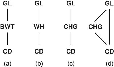
Graphs constructed using different HPD interval content for the decisions of the IC algorithm are depicted in Figure 1. For two triplet sets of traits including GL, CD and BWT, and GL, CD and WT, the IC algorithm with all HPD intervals resulted in one graph each (Figure 1a and b), which had links between GL and BWT (WH) and between BWT (WH) and CD. On the other hand, applying 95% and 90% HPD intervals for another triplet including CHG detected the same structure as the two triplets including BWT or WH (Figure 1c), but using 85% and 80% HPD intervals recovered an extra link between GL and CD (Figure 1d). However, the directions of the links were not resolved in any of the graphs.
Links between traits detected by the inductive causation algorithm with 95% to 80% (a and b), 95% and 90% (c) and 85% and 80% (d) of highest posterior density intervals. GL=gestation length; CD=calving difficulty; BWT=birth weight; WH=withers height; CHG=chest girth.

The structural equation model analysis based on the results from the IC algorithm
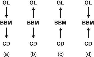
To fit the structural equation model for a causal structure, we assigned directions between the links detected by the IC algorithm based on graph theory. Possible causal structures based on the links between traits were depicted in Figure 2a (GL→BBM→CD), 2b (GL←BBM→CD) and 2c (GL←BBM←CD), as the three models are statistically equivalent (Valente et al., Reference Valente, Rosa, Gianola, Wu and Weigel2010). Here, birth body measurements (BBM) represents BWT, WH or CHG. The causal structure depicted in Figure 2d (GL→BBM←CD) cannot be assumed, because it has an unshielded collider that should already be detected by Step 2 in the IC algorithm. The causal network shown in Figures 2a and b were chosen for fitting the structural equation model, because CD would never affect BWT, WH or CHG biologically.
Possible causal structures based on the links between traits detected by the inductive causation algorithm (a to c), except for (d). GL=gestation length; CD=calving difficulty; BBM=birth body measurements including birth weight, withers height or chest girth.

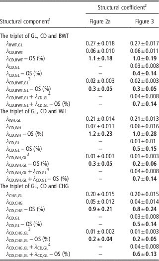
Posterior means of structural coefficients obtained from the structural equation model fitted to the causal structure GL→BBM→CD (Figure 2a) are shown in Table 5. The inferred structural coefficients were all significantly different from zero (P<0.05). In the triplet of GL, CD and BWT, the structural coefficients of GL on BWT (λ BWT,GL) and of BWT on CD (λ CD,BTW) were 0.27 and 0.06, respectively. On the other hand, the coefficients of BWT on CD (λ CD,BTW) from the structural equation model with the structure of GL←BWT→CD (Figure 2b) was 0.06 (Supplementary Table S1) and the same as the corresponding λ CD,BTW (0.06) from the structural equation model with the structure of GL→BWT→CD (Figure 2a). Similarly, the coefficients of BWT on GL (λ GL,BWT) of Figure 2b (0.28, Supplementary Table S1) and λ BWT,GL of Figure 2a (0.27) were the almost same. Likewise, in the triplets including WH or CHG, the coefficients inferred from the structure in Figure 2a and b were similar.
Posterior means±posterior standard deviations of the structural coefficients resulting from the structural equation model

GL=gestation length; CD=calving difficulty; BWT=birth weight; WH=withers height; CHG=chest girth; OS=observable scale.
1 λ=structural coefficient, λ i,j denotes a structural coefficient from the jth trait to the ith trait.
2 Structural coefficients resulting from the structural equation models with the structures of Figures 2a (based on the results from the inductive causation algorithm) and 3 (based on biological prior knowledge). 95% highest posterior density region of all structural coefficients does not include 0. Structural coefficients on the observable scale were represented in bold font.
3 Indirect structure effect of GL through the mediating effect of BWT (WH, CHG) on CD, which is calculated as the product of the structural coefficients λ BWT (WH, CHG),GL×λ CD,BWT (WH, CHG).
4 Overall effect of GL on CD, which is the sum of the direct and indirect structure effects.
It is well known that the fetus triggers the onset of parturition by initiating a series of complex endocrine and biochemical events. During the final stage of gestation, fetal mass approaches the inherent space limitations of the uterus. As a result, the fetus becomes stressed, which causes the fetal anterior pituitary to release adrenal corticotrophin. It stimulates the fetal adrenal cortex to produce corticoids. The elevation of fetal corticoids initiates a series of events for changes in the endocrine condition of the dam (Senger, Reference Senger2005). According to this biological mechanism, larger body size, including a part of heavier BWT of a calf against its dam’s size should cause shorter GL (negative relationship) and not a longer one (positive relationship). Hence, the positive causal coefficients for BWT, WH or CHG on GL (Figure 2b, Supplementary Table S1) inferred in this study were not appropriate biologically. Therefore, only the result from the structural equation model fitted to the causal structure GL→BBM→CD (Figure 2a) are shown hereafter, and posterior means and PSD of the variance components within each trait from the model are shown in Supplemental Table S2.
The structural coefficients of λ BWT,GL and λ CD,BWT from the structural equation model in Figure 2a were 0.27 and 0.06, respectively, and OS for λ CD,BWT was 1.1% (Table 5). This means that an extra day of GL results in a gain of 270 g in BWT and 1 kg of BWT increases the risk of dystocia by 1.1%. Indirect structure effect of GL through the mediating effect of BWT on CD (λ CD,BWT,GL) was smaller (0.02% and 0.3% on OS) than the direct effects of GL on BWT (λ BWT,GL) and BWT on CD (λ CD,BWT). The indirect effect was calculated as the product of the structural coefficients λ BWT,GL×λ CD,BWT (Shipley, Reference Shipley2016). Lopez de Maturana et al. (Reference Lopez de Maturana, Wu, Gianola, Weigel and Rosa2009) estimated 0.06% to 0.47% of direct recursive effect of GL on CD (λ CD,GL) on the OS, using a subgroup of GL in Holstein cows. This means that an extra day of GL increases the risk of dystocia by 0.06% to 0.47%. The structure effect of GL on CD on OS (λ CD,BWT,GL−OS=0.3%) was within the range of their estimates, although the structural effect in our study was indirect effect through the mediating effect of BWT.
In the triplet including WH, an extra day of GL results in a growth of 2.1 mm in WH and 1 cm of WH increases the risk of dystocia by 1.2%. Similarly, CHG grows by 2.0 mm/day of GL and raises the CD by 0.9%, by increasing the CHG by 1 cm. Although these estimates had similar magnitudes to those from the analysis including BWT, as described above (Table 5), the effects of GL on WH and CHG per unit seemed to be weaker than on BWT. On the other hand, the effect of WH and CHG ‘per unit’ on CD could be larger than that of BWT, because coefficient of variations (CVs) for WH and CHG were smaller than that for BWT (Table 2). Conversely, however, this means that WH and CHG would hardly have a big influence on CD at the same time, owing to their smaller CV. Indirect structure effects of GL through the mediating effects of WH and CHG on CD (λ CD,WH,GL and λ CD,CHG,GL) in original and observed scale were almost the same as those of λ CD,BWT,GL.
The structural equation model analysis based on biological prior knowledge
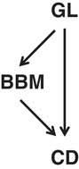
We have shown the results of causal association among the traits resulting from the IC algorithm. However, by taking into account biological prior knowledge, an extra causal relationship between GL and CD could be considered. In addition, applying the IC algorithm with 85% and 80% HPD intervals for the triplet including CHG detected an extra link between GL and CD (Figure 1d). Therefore, we also fitted the structural equation model to alternative structures (Figure 3) which have a directed link from GL to CD, or GL→CD (λ CD,GL), based on biological prior knowledge about the relationship between the traits, on the structure shown in Figure 2a. Posterior means of the structural coefficients resulting from the structural equation model fitted to the causal structure (Figure 3) is also shown in Table 5. In the triplet including BWT, λ BWT,GL, λ CD,BTW and its OS were 0.27%, 0.06% and 1.0%, respectively. Moreover, they were found to be almost identical to the corresponding structural coefficients from the structural equation model with the structure of Figure 2a. In addition, indirect structure effect of GL through the mediating effect of BWT on CD (λ CD,BWT,GL) and its OS were the same in both the structural equation models (0.02% and 0.3%, respectively). The added direct recursive causal effect of GL on CD (λ CD,GL) and its OS were 0.03% and 0.4%, respectively. The overall effect of GL on CD (λ CD,BWT,GL+λ CD,GL), which is the sum of the direct and indirect structure effects and λ CD,GL+λ BWT,GL×λ CD,BWT (Shipley, Reference Shipley2016), and its OS were 0.04% and 0.7%, respectively. The direct causal effect of the extra link (λ CD,GL), which was not detected by the IC algorithm, was similar to the indirect causal effect of GL through the mediating effect of BWT on CD (λ CD,BWT,GL), and was significant (P<0.05). The magnitude of the estimate for such a link should generally be close to zero or non-important. This could be due to the application of the IC algorithm to the variances from the sire-MGS model in this study, and maternal genetic effect might not have been removed completely from the residual variance components as Valente et al. (Reference Valente, Rosa, Gianola, Wu and Weigel2010) pointed out.

Bellows et al. (Reference Bellows, Short, Anderson, Knapp and Pahnish1971) studied the factors that affect CD and BWT in Angus and Hereford heifers by standard partial regression. They found a highly significant positive effect of BWT on CD (0.50 and 0.65 for Angus and Hereford, respectively), no effect of GL on CD (0.04 and −0.05) and a significant positive effect of GL on BWT (0.30 and 0.20). The results of the causal relationships among the traits from the structural equation model in this study were consistent with their results except for the effect of GL on CD, although their results were not conditional on genetic effects, or were just from phenotypic associations.
In the triplets including WH or CHG, the structural coefficients and their OSs from the structural equation models with the structure of Figure 3 were almost the same with the corresponding structural coefficients from the structural equation models with the structure of Figure 2a. The direct causal effect of GL on CD (λ CD,GL), the overall effect of GL on CD and their OSs were almost the same with those in the triplet including BWT. The added direct causal effect of GL on CD (λ CD,GL) in the triplet including CHG was not different from that in the triplets including BWT or WH, although applying 85% and 80% HPD intervals in the IC algorithm recovered an extra link between GL and CD, only in the triplet including CHG.
Conclusions
The IC algorithm could not detect any directed edges in the present study, and thus we had to refer biological knowledge to direct the detected edges between the traits. Nonetheless, the causal inference still helps us to detect the causal networks between the traits. For example, the IC algorithm inferred the structure GL – BWT – CD in our result. However, if we assume the causal structures for the three traits just based on biological knowledge, the structures could also be GL→CD←BWT, BWT→GL→CD and so on. Number of traits of interest in the present study was only three. In practical scenarios, increasing the number of traits of interest increases the number of combinations of the traits and would be too complicated to decide the causal structure among them just based on prior knowledge. The IC algorithm searches for minimal causal structures and provides clues of causal networks among traits. Applying the structural equation model revealed phenotypic causal associations between GL, CD and calf size (BWT, WH or CHG). The analyses for the three triplets resulted in almost the same estimates for the structural coefficient. However, the impacts of the causal effects would be different because the unit of each trait was different. The structural equation model was also fitted to the causal structure, which had an extra link based on biological prior knowledge. The causal effect of the extra link (λ CD,GL) was similar magnitude to the indirect causal effect (λ CD,BBM,GL) recovered by the IC algorithm and was significant (P<0.05), although the other causal effects of links corresponding to both structures were almost the same. This suggest that maternal genetic effects might not be removed completely from the residual variance components in the sire-MGS model, and the application of the IC algorithm to the variance components from the model could lead to detecting an incorrect structure. Nonetheless, fitting the structural equation model to the causal structure provided useful information such as the magnitude of the causal effects between GL, CD and calf size.
Acknowledgments
This work was supported by a grant from the Ministry of Agriculture, Forestry and Fisheries of Japan (Development of Breeding Technology for Animal Life Production).
Supplementary materials
To view supplementary material for this article, please visit https://doi.org/10.1017/S1751731117000957