1. Introduction
Climate change will potentially transform the physical and human geography of the planet, but the nature of this process is still uncertain. Changes in temperature levels and rainfall variability depend on how the global climate system adjusts to increasing greenhouse gas (GHG) concentrations, with variable impacts across regions and economic sectors (Stern, Reference Stern2008). Due to its direct dependence on temperature and rainfall, the agricultural sector is one of the sectors most vulnerable to climate change (Deschênes and Greenstone Reference Deschênes and Greenstone2007).
Although there is no consensus on the exact impact of climate change on agriculture, it is usually accepted that developing countries, such as Brazil, will be more negatively affected. The primary explanation for this is that developing countries are located predominantly at low latitudes. In these areas, temperatures are already hot, occasionally above the optimum levels for agriculture. In low latitudes, the rural poor tend to live in the hotter and drier regions of each country. Global warming is likely to damage these regions more severely than each country's more temperate zones. Moreover, according to Cline (Reference Cline2007) and Stern (Reference Stern2007), a reduction in agricultural potential would lead to higher losses for developing economies than for developed economies because the agricultural sector accounts for a significant portion of income in developing nations.
According to Seo and Mendelsohn (Reference Seo and Mendelsohn2008a), to adequately quantify the impacts of climate change on agriculture, one must take into account adaptation strategies. The analysis cannot simply estimate how current conditions will be affected. The forecasts must also capture crop switching; that is, they should recognize that producers will change their production decisions to maximize profit according to each climate scenario. Studies that assume that producers will continue performing the same activities without changing their production technologies surely overestimate losses.
Planning for climate adaptation necessarily requires comparisons of different alternatives, accounting for the possibilities and limitations of each technology as well as for the uncertainties associated with climate change (Pidgeon and Fischhoff, Reference Pidgeon and Fischhoff2011). According to Magrin et al. (Reference Magrin, Garcia, Choque, Gimenez, Moreno, Nagy, Carlos, Villamizar, Parry, Canziani, Palutikof, Van Der Linden and Hanson2007) and Seo (Reference Seo2011), irrigation is a major adaptation measure used by farmers in Latin America and elsewhere to counteract the negative impact of climate change. Irrigation increases crop productivity and minimizes the impact of water stress on agricultural production.
Irrigation could be a powerful adaptive strategy in Brazil due to the availability of water and suitable soils. The country holds approximately 12 per cent of the fresh water reserves of the planet. Furthermore, according to the Agricultural Census (IBGE, 2006), Brazil has approximately 30 million hectares of soil suitable for the sustainable developmentFootnote 1 of irrigated agriculture, with only 4.4 million ha currently being cultivated with irrigation systems and technologies.
In this context, this study seeks to conduct an analysis of climate change effects on Brazilian agriculture by considering irrigation as an adaptive strategy. The objective is to investigate how key climatic variables influence irrigation adoption and how farm decisions to adapt to climate alterations affect land valuesFootnote 2 in different regions of Brazil. According to Di Falco et al. (Reference Di Falco, Veronesi and Yesuf2011), this type of analysis is particularly important because most of the discussion about agriculture and climate change fails to consider the role of adaptation.
The main studies that have analyzed climate change impacts on Brazilian agriculture (Siqueira et al. Reference Siqueira, Farias and Sans1994; Sanghi et al. Reference Sanghi, Alves, Evenson and Mendelsohn1997; Nobre et al., Reference Nobre, Assad and Oyama2005; Ávila et al., Reference Ávila, Irias and Lima2006; Embrapa Reference Embrapa2008) unanimously state that climate change will negatively impact the country. They also agree that the various regions will be affected differently, which is directly related to the substantial variation in climatic conditions throughout the nation. However, with the exception of the analysis of change in land use by Evenson and Alves (Reference Evenson and Alves1998), none of these studies considered adaptation, which may lessen the adverse impacts of climate change.
The role of irrigation as an adaptation strategy in agriculture has been analyzed in other studies. Some of the previous studies estimate separate response functions for rainfed and irrigated agriculture (Schlenker et al. Reference Schlenker, Hanemann and Fisher2005; Kurukulasuriya and Mendelsohn Reference Kurukulasuriya and Mendelsohn2008; Seo and Mendelsohn, Reference Seo and Mendelsohn2008b). These studies assume that irrigation is an exogenous variable. Nevertheless, irrigation is sensitive to climate and will change as climate changes (Kurukulasuriya et al. Reference Kurukulasuriya, Kala and Mendelsohn2011; Seo Reference Seo2011). We take this fact into account using a treatment effect model. Therefore, by explicitly including irrigation as an endogenous variable, we can better understand the impacts of climate change on the domestic agricultural sector and contribute more effectively to future public policies aimed at creating strategies to combat the effects of global warming on agriculture.
It is important to emphasize that our paper shares common characteristics with Seo (Reference Seo2011). The author considers the irrigation decision as an adaptation strategy and analyzes climate change impacts on the South American agricultural sector (data covered Argentina, Chile, Colombia, Ecuador, Venezuela and Brazil). In his paper, the author showed that both irrigated and rainfed agriculture will be negatively affected, but the latter will be more severely affected. Seo's study represented a very important contribution to the understanding of climate change impacts in South America. However, the author did not show how each country may be affected and the potential regional differences within countries.
Therefore, a particular analysis for the Brazilian case is important because Brazil displays distinct characteristics relative to its Latin American neighbors and other countries. Due to the country's size, geographic position and climate, agricultural production in Brazil is diversified and heterogeneous: agriculture practiced in the South is very different from that practiced in the North. Furthermore, Brazil has a well-defined policy on climate change and has been allocating specific resources for adaptation activities in agriculture. All of these factors make Brazil's capacity for adaptation to climate change different from that of its neighbors, which requires more focused analysis.
In addition, Brazil has an important role regarding future food and fiber supply. According to Tollefson (Reference Tollefson2010), Brazilian agricultural production will grow much faster than in other countries. During the last decade, Brazil's beef exports increased more than 300 per cent and Brazil became the second major soybean exporter. However, this outstanding performance could be jeopardized by climate change. Thus, we believe that this paper presents an important contribution to the literature on climate change impact by examining the potential role of irrigation in decreasing Brazilian agriculture vulnerability to climate change.
The paper proceeds as follows. The next section describes the methodological framework. In the third section, a detailed description of the data sources and variables is provided. Next, the empirical results are presented and discussed. In the last section, a summary, several conclusions and a discussion about policy are provided.
2. Methodological framework
In this paper, a hypothesis will be tested that the practice of irrigation tends to increase agricultural land values and that irrigation has the potential to mitigate the negative effects of global climate change on the Brazilian agricultural sector. To verify this statement, the analytical model assumes that the adoption of irrigation or the continued use of dryland production practices is made by producers to maximize their profits. The decision to produce under irrigation is an alternative to dryland production and is assumed to be discrete: either the irrigation system is installed or it is not installed.
In Brazil, most investments in irrigation projects are conducted by the private sector. Although the government performs an important role in this process by providing loans and funding to farmers, public projects represent only 4–6 per cent of the irrigated area of the country and are geographically concentrated in northeastern Brazil (a semi-arid region) (Ministério da Integração Nacional, 2008). In public irrigation areas, the government provides each agricultural establishment with the infrastructure needed for water supply. However, the farmer is responsible for assembling the irrigation conveyance and application system that he will use as well as for the selection of the crops that he will produce. After the beginning of production, farmers must manage the irrigation area and pay tariffs. These tariffs should be sufficient to maintain the common infrastructure and also to repay the public investment. Ultimately, even though the public sector builds the initial infrastructure, all investment costs are eventually paid by the beneficiary farmers (Thomé and Castro et al. Reference Thomé e Castro, Neves and Nakatani2013). Therefore, in this study, irrigation is characterized as a private adaptive measure of farmers and not deliberately promoted by the government.
The profit-maximizing producer i will install the infrastructure for irrigation if the profits under irrigation are greater than under dryland production. This decision is part of a process of maximizing benefits that ensures that only optimal choices are observed. Therefore, the choice is not an exogenous variable but an endogenous decision influenced by the environment in which the producer is situated, which includes soil types, temperature, rainfall, producer's technology and management practice regime, economic conditions, etc. The irrigation adoption decision is voluntary and based on individual self-selection.
According to Di Falco et al. (Reference Di Falco, Veronesi and Yesuf2011), it is possible that irrigators may differ from dryland farmers in various respects and that farmers may have decided to adopt irrigation based on expected benefits that differ across populations. Unobservable characteristics of producers and their farms may affect both irrigation decisions and their profitability. To account for the endogeneity of irrigation adoption, a simultaneous equations model with endogenous switching (originally developed by Maddala and Nelson, Reference Maddala and Nelson1975 and Maddala Reference Maddala1983) was employed.
Following Di Falco et al. (Reference Di Falco, Veronesi and Yesuf2011), consider a population of farmers, each of whom voluntarily chooses whether to adopt irrigation technologies. Let the latent variable A i * represent the expected benefits of irrigated production with respect to dryland production. The selection equation for irrigation adoption is as follows:
 $$A_i^{\ast} = E_i \alpha + \varepsilon_i$$
where the observed farmer decision is A i = 1 if he adopts irrigation (A i * > 0), A i = 0 otherwise, and E is a vector of exogenous variables that determine the decision, such as soil and climatic characteristics, and the socioeconomic features of producers.
To evaluate the impact of the self-selection process on Brazilian land values, an endogenous switching regression model was adopted. The model accounts for the fact that the expected land values may depend on irrigation adoption. Producers face two regimes, (1) irrigation adoption and (2) dryland production, which are defined as follows:
 $$\Pi_{1i} = Z_{1i} \beta_1 +\mu_{1i} \quad {\rm if} \quad A_i = 1$$
 $$\Pi_{2i} = Z_{2i} \beta_2 + \mu_{2i} \quad {\rm if} \quad A_i = 0$$
where ∏1i and ∏2i refer to land values in regimes (1) and (2), i.e., irrigated production and dryland, respectively, where Z i is a vector of exogenous variables that influence land values and therefore includes climatic conditions, and where μ1i and μ2i are the terms of random errors.
By assumption, the error terms are assumed to have a trivariate normal distribution with a zero mean and the covariance matrix Σ, i.e., (μ1, μ2, ε1)~N(0, Σ):
 $$\Sigma = \left[\matrix{\sigma_{\varepsilon^2} & \cdot & \cdot \cr \sigma_{1\varepsilon} &\sigma_1^2 &\cdot \cr \sigma_{2\varepsilon} & \cdot &\sigma_2^2} \right]\comma \;$$
where σε 2 is the variance of the error term in the selection equation (1), σ1 2 and σ2 2 are the variances of the error terms in the profit functions (2a) and (2b), σ1ε and σ2ε represent the covariance of ε i , μ1i and μ2i , and the covariance between μ1i and μ2i is not defined, as Π1i and Π2i are never observed simultaneously (Maddala, Reference Maddala1983; Di Falco et al. Reference Di Falco, Veronesi and Yesuf2011).
The error term of the selection equation (1) is correlated with the error term of the profit functions (2a) and (2b). Because of this correlation, the expected values of μ1i and μ2i that are conditional on the sample selection are different from zero:
 $$\eqalign{E \left(\mu_{1i} \left\vert A_i =1 \right. \right)&=\sigma_{1\varepsilon} {\phi \left(E_i \alpha \right)\over \Phi \left(E_i\alpha \right)} = \sigma_{1\varepsilon} \lambda_{1i}\cr E \left(\mu_{2i} \left\vert A_i =0 \right. \right)& = -\sigma_{2\varepsilon} {\phi \left(E_i\alpha \right)\over 1 - \Phi\left(E_i \alpha \right)} = \sigma_{2\varepsilon} \lambda_{2i}}$$
where Φ(.) is the standard normal cumulative density function, ϕ(.) is the standard normal probability density function, and
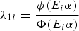 $\lambda_{1i} = {\phi \lpar E_{i} \alpha\rpar \over \Phi \lpar E_{i} \alpha\rpar }$
and
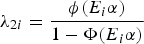 $\lambda_{2i} = {\phi\lpar E_{i}\alpha\rpar \over 1 - \Phi \lpar E_{i} \alpha\rpar }$
.
If the estimated covariances
 $\hat{\sigma}_{1\varepsilon}$
and
 $\hat{\sigma}_{2\varepsilon}$
are statistically significant, then irrigation adoption and land values are correlated. Thus, there is evidence of endogenous switching, and the null hypothesis of absence of sample selectivity is rejected.
Given the assumption with respect to the distribution of the disturbance terms, the efficient method for estimating endogenous switching regression models is the full information maximum likelihood (FIML) (Lee and Trost, Reference Lee and Trost1978; Di Falco et al., Reference Di Falco, Veronesi and Yesuf2011). The logarithmic likelihood function for the system of (1–3) is
 $$\eqalign{\ln L_i &=\sum_{i = 1}^N A_i \left[\ln \phi \left({\mu_{1i} \over \sigma_1} \right)- \ln \sigma_1 + \ln \Phi \left(\theta_{1i} \right)\right]\cr &\quad + \left(1 - A_i \right)\left[\ln \phi\left({\mu_{2i} \over \sigma_2} \right)- \ln \sigma_2 + \ln \left(1 - \Phi \left(\theta_{2i} \right)\right)\right]}$$
where
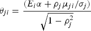 $\theta_{ji} = {\lpar E_i \alpha +\rho_j \mu_{ji}/\sigma_j\rpar \over \sqrt{1 - \rho_j^2}}$
, j = 1, 2 and ρ
j
is the correlation coefficient between the error terms ε
i
(selection equation) and μ
ji
(regimes equations).
After estimating the model's parameters, the endogenous switching regression model can be used (a) to compare the expected land values of the irrigators (b) with respect to the dryland farmers and (c) to analyze the expected land values in the counterfactual hypothetical cases that the irrigator did not adapt and (d) that the dryland farmer did adapt (Di Falco et al. Reference Di Falco, Veronesi and Yesuf2011). These four cases are defined as follows:
 $$E\left(\Pi_{1i} \left\vert A_i = 1 \right. \right)=Z_{1i} \beta_1 + \sigma_{1\varepsilon} \lambda_{1i}$$
 $$E\left(\Pi_{2i} \left\vert A_i = 0 \right. \right)= Z_{2i} \beta_2 +\sigma_{2\varepsilon} \lambda_{2i}$$
 $$E\left(\Pi_{2i}\left\vert A_i = 1 \right. \right)= Z_{1i} \beta_2 + \sigma_{2\varepsilon} \lambda_{1i}$$
 $$E\left(\Pi_{1i}\left\vert A_i = 0 \right. \right)= Z_{2i} \beta_1 + \sigma_{1\varepsilon} \lambda_{2i}.$$
According to Di Falco et al. (Reference Di Falco, Veronesi and Yesuf2011), cases (a) and (b) represent the actual expectations observed in the sample. Cases (c) and (d) represent the counterfactual expected outcomes.
Based on the estimated land values for the three systems, it is possible to calculate their changes resulting from climate change. We follow Seo (Reference Seo2011) to measure the effect of climate change, from C 1 to C 2, in land values Δ∏ i :
 $$\Delta \prod\nolimits_i = \Pi_1 \lpar C_2\rpar - \Pi_1 \lpar C_1\rpar.$$
We used values of temperature and precipitation for three time periods (2020, 2050 and 2080) under two different climate scenarios (A1B and A2) presented in the International Panel on Climate Change Fourth Assessment Report. The option for the A1B and A2 scenarios was based on Le Quéré et al. (Reference Le Quéré, Raupach, Canadell and Marland2009), who show that the current GHG emissions are closer to scenarios A1/A2 than to scenarios B, which in turn are considered unrealistic in the present. Following Oliveira et al. (Reference Oliveira, Costa, Soares-Filho and Coe2013), to avoid individual model biases, we used the average of 10 Atmospheric-Oceanic General Circulation Models (AOGCMs).Footnote 3 According to these authors, the average of the climate variables from different climate models is likely to be more representative than the estimates of any individual model.
3. Variables and data
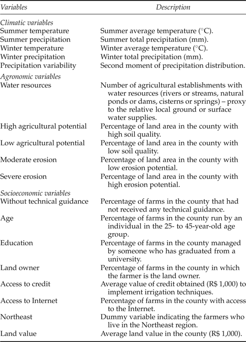
To compose the Z vector, three categories of variables were used: socioeconomic, agronomic and climatic (table 1). The unit of observation was the Minimum Comparable Area (MCA), which refers to the aggregated area of the smallest number of counties needed to ensure the comparisons of a same geographical area from different time periods. Because MCAs represent county-level observations, we will simplify the exposition by referring to them as ‘counties’.Footnote 4
Variables description

Socioeconomic variables, including features related to education, age, income and access to water resources,Footnote 5 as well as variables related to land use, such as the use of either irrigation or rainfed technologies, were obtained from the 2006 Agricultural Census, published by the Instituto Brasileiro de Geografia e Estatística (IBGE). The agronomic data included the variables of soil (i.e., agricultural potential) and erosion potential, which were provided by the Núcleo de Estudos e Modelos Espaciais Sistêmicos (NEMESIS). These variables were created by overlaying geo-referenced county boundaries over geo-referenced land-attribute data.Footnote 6
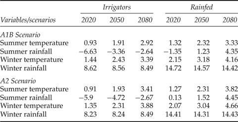
Information about observed temperatures and precipitation rates were extracted from the CL 2.0 10' dataset produced by the Climate Research Unit (CRU)/University of East Anglia. The observed climate variables were temperature (°C) and precipitation (mm/month) for the period 1961–1990. We used two seasonal means: December through February (summer) and June through August (winter) using monthly values. According to Féres et al. (Reference Féres, Reis and Speranza2008), ‘this seasonal specification decreases the information loss associated with the conventional use of one month from each season and simultaneously maintains a measure of the trends in intra-annual variation’. To construct the variables, the NEMESIS converted all climate data into arcGIS shapefiles using their XY coordinates, and these grid-points were joined with the MCA boundaries layer with the average temperature and precipitation values being calculated for each MCA (Féres et al., Reference Féres, Reis and Speranza2008). Unlike the analyses that have already been conducted on these data, which have included only the first moments of climatic variables distribution, climate variability was considered in our study by including the second moments of precipitation distribution. Finally, data on projected climate change was provided by the NEMESIS and cover two representative scenarios that span the range of predictions for Brazil (Appendix, table A1).
It is important to note that the decision to consider only summer and winter temperatures and rainfalls instead of those of all four seasons was based on studies by Seo and Mendelsohn (Reference Seo and Mendelsohn2008a) and Seo (Reference Seo2010, Reference Seo2011). According to the authors, such a specification is more appropriate for studies of South America because this region does not have four well-defined seasons, unlike the USA.Footnote 7
The dummy variable indicating the adoption of irrigation (A i ) was built from the data on irrigated area in Brazilian counties. According to the 2006 Agricultural Census (IBGE, 2006), the irrigated area in Brazil accounts for 7.4 per cent of total Brazilian cropland. Therefore, we consider A i = 0 whether the county had less than 7.4 per cent of total cropland irrigated and A i = 1 otherwise. The dependent variable of the endogenous switching regression model was land value. This variable, which was provided by the 2006 Agricultural Census (IBGE, 2006), is measured in terms of monetary units (R$ 1,000). Land values represent farmers' best estimations of the value of their cropland without any improvements, such as buildings.
Following Schlenker et al. (Reference Schlenker, Hanemann and Fisher2005), we omit all urban counties because the strong influence of urbanization on farmland values in these counties could cause bias. We excluded 436 counties (the original sample consisted of 3,660 municipalities) based on the study ‘Urban-Regional Division’ conducted by the IBGE. This study is a contribution of the IBGE to the analysis of the Brazilian territorial dynamics, offering a regional view of Brazil based on the connectivity of urban flows. The identification and delimitation of the Areas of Urban Connectivity were strongly intertwined with an understanding of social/spatial transformations taking place in the country.
4. Results and discussion
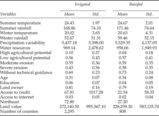
We start by examining the descriptive statistics of the variables presented by the two types of agricultural production systems – irrigated and rainfed – shown in table 2. Mean temperature did not show significant differences. Differences between rainfed and irrigated production can be observed only in precipitation variables. Irrigated production was exposed to high precipitation variability and a lower mean volume of rainfall, and this difference was more significant during winter. This difference, although not very high for Brazil as a whole, becomes considerably greater when we consider different regions because the country has large climate variability (which explains the high standard deviation). In the Northeast, for example, where the greatest effects of climate change are expected (Marengo et al., Reference Marengo, Nobre, Chou, Tomasella, Sampaio, Alves, Obregón, Soares, Betts and Kay2011), the average rainfall for irrigators during summer is 85.7 mm, while for rainfed farmers, it is 102 mm. Therefore, where precipitation is abundant, farmers tend to practice rainfed agriculture, but as the conditions become drier, there is a gradual shift to irrigated systems. Similar results were found by Seo (Reference Seo2011), who examined irrigation in Latin America.
Descriptive statistics on agricultural production in Brazil

Notes: In this table, the values indicate the percentages for irrigated and rainfed counties. Land values and Access to Credit are represented in R$ 1,000. Northeast is a dummy variable indicating the farmers who live in the Northeast region.
It is import to emphasize, from an agronomic point of view, that drought or soil water deficit can be chronic in climatic regions with low water availability during the period of plant growth (Tyree, Reference Tyree, Pugnaire and Valladares2007; Nobel, Reference Nobel2009; Harb et al., Reference Harb, Krishnan, Ambavaram and Pereira2010). For example, for rainfed farmers who plant soybeans, there are high risks of losses if there is a drought event during the critical stages of plant development, such as pod development and seed fill. A single irrigation during pod elongation increases the number of seeds per plant, while irrigation at seed enlargement stage increases seed weight, resulting in increased yield (Sweeney and Granade, Reference Sweeney and Granade2002). Thus, even if precipitation is a few millimeters less, representing a difference of 11 per cent for the variable Winter Rainfall (table 2), it justifies irrigation.
Minor differences can also be observed in the agronomic and socioeconomic variables. Rainfed producers had less access to water (groundwater or surface water supplies, including rivers or streams, natural ponds or dams, cisterns or springs) and were located in counties with low soil quality. The share of farms without technical guidance (publicly funded or not) was lowest among irrigators who also had greater access to the Internet and credit. In general, it is expected that rainfed producers with these advantages are more likely to adopt irrigation.
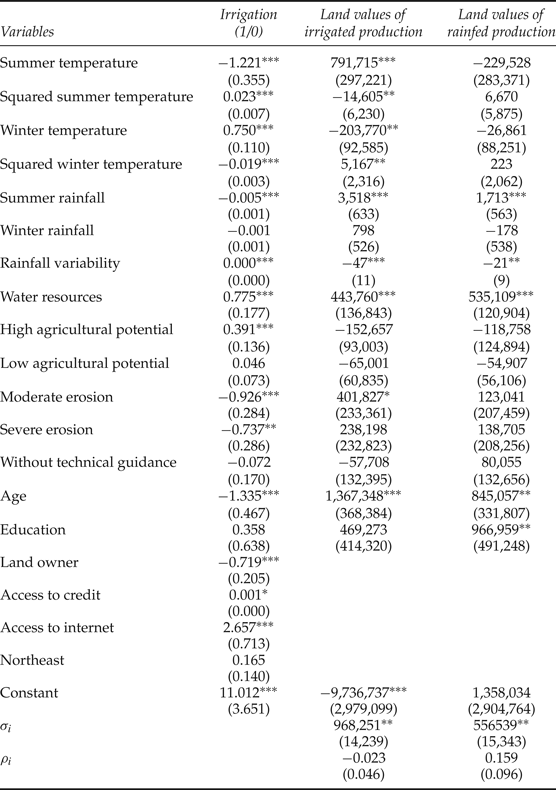
Following the proposed methodology, the first part of the analysis consists of employing an endogenous switching regression model with FIML (table 3). The first column presents the estimated coefficients of the selection equation of whether to irrigate or not irrigate, and the second and third columns show the land values for each type of agricultural production system.
Parameters for estimates of irrigation adoption and land values

Notes: Standard errors in parentheses. ***, ** and * indicate significance at the 1%, 5% and 10% levels, respectively.
It is important to note that it is necessary to include a set of instruments that help identify the model (Lokshin and Sajaia, Reference Lokshin and Sajaia2004). We used four variables as selection instruments in the land value equations. These variables are the percentage of farmers who are landowners in the county (‘Land Owner’), the average value of credit obtained to implement irrigation techniques (‘Access to Credit’), the percentage of farmers with Internet access (‘Access to Internet’), and a dummy variable indicating the farmers who live in the Northeast region (‘Northeast’).Footnote 8
To verify the admissibility of these instruments, we perform a test for overidentification (Hansen's J test) based on the two-stage least squares (TSLS) estimator. According to Di Paolo and Raymond (Reference Di Paolo and Raymond2012) and Cameron and Trivedi (Reference Cameron and Trivedi2010), the endogenous switching model and the TSLS estimator are similar methods for addressing an endogenous dummy variable (irrigation, in our case). Thus, we used TSLS to understand whether the chosen instruments are valid. The value of the Hansen's J test was 5.5246 (p-value of 0.0631), which suggests that the instruments are likely to be valid at the 1 per cent or 5 per cent significance levels.Footnote 9
The results of the selection equation indicate that agronomic, socioeconomic and climatic conditions influence irrigation adoption in Brazil. Access to information (represented by the InternetFootnote 10 variable) and water resources are important drivers of irrigation adoption. The availability of land in good condition for agricultural production is also relevant. It is important to highlight that the negative sign for the variable ‘land owners’ was not expected. The prior expectation, as established in the literature, was that the higher the number of owners in a county, the greater the likelihood of irrigation. However, following the reasoning of Moffatt (Reference Moffatt2005), just because a land owner is likely to be a potential irrigator does not mean he will therefore irrigate. There may be a proportion of the population of farmers who would, out of principle, never irrigate under any circumstances. In addition, for most Brazilian farmers, investment requirements and costs of administration, operation and maintenance of the irrigation system are very high. In other words, the opportunity cost of spending on the irrigation system is high, which could explain the non-adoption of the system even for those who are land owners. This fact may explain the small number of irrigators in the country (6.4 per cent of farmers). According to the Agricultural Census (IBGE, 2006), the share of land owners who are irrigators is 7.76 per cent, while the share of non-owners (partners, tenants, occupiers, etc.) who use irrigation is 7.91 per cent. From a mean comparison t-test, it can be observed that these means are not significantly different.
Except for winter rainfall, all climate coefficients are significantly different from zero. This result indicates that, similar to the reports of (Mendelsohn and Seo, Reference Mendelsohn and Seo2007), Kurukulasuriya et al. (Reference Kurukulasuriya, Kala and Mendelsohn2011), Seo (Reference Seo2011) and Cunha et al. (Reference Cunha, Coelho, Féres and Braga2014), irrigation adoption is sensitive to both temperature and precipitation, which validates its utility as an adaptive strategy.
An analysis of the linear and quadratic terms of the summer temperature variable indicated a U-shaped behavior. Therefore, if temperatures rise, the irrigation probability decreases to a minimum level before increasing. This pattern can be attributed to certain characteristics of the summer climate. In Brazil, temperature increases are followed by increasing rainfall during summer. In addition, the amount of water input in an agriculture system depends on its species, cropland, soil type, sowing date and stage of plant development. During the seed maturation and germination stages, as well as during the initial seedling growth, conditions of excess soil water can be harmful to plants because it can lead to soil humidity increases and cause the accumulation of fungus and other pathogens (Negri et al., Reference Negri, Gollehon and Aillery2005).
Taking this risk into consideration, it is well known that irrigation is a widespread strategy adopted for meeting the water requirements of crops and that high temperatures can have different effects depending on the soil humidity. Hence, if the soil water content available to plant growth is kept constant, a decrease in the irrigation requirements can be observed even when the temperature increases. However, if the environment becomes warmer and exceeds the optimum growth temperature, plant development is likely to be impaired. Thus, an increase in irrigation seems to be an alternative measure for mitigating the adverse effects of high temperatures.
For winter temperatures, the data indicate an opposite pattern. Increased temperature increases the probability of irrigation up to a maximum value before decreasing. This result is similar to Mendelsohn and Seo (Reference Mendelsohn and Seo2007) and Seo (Reference Seo2011). Whereas irrigation decisions are made before the plant growing season and are based on the weather conditions expected for the period, it is reasonable that a higher predisposition to irrigation occurs when higher temperatures are expected. However, as stated by Mendelsohn and Seo (Reference Mendelsohn and Seo2007), for certain temperature thresholds, the expected irrigation profitability becomes less significant, as plants have heat tolerance limits. Thus, irrigation efficiency decreases and the gains may not compensate for its costs.
The results present the expected behavior for the rainfall variables. As rainfall increases, the probability of irrigation decreases. Irrigation is used as a response to water scarcity and thus is central to yield gains. However, as highlighted by Mendelsohn and Seo (Reference Mendelsohn and Seo2007), the marginal contribution of irrigation to the profitability of producers decreases as rainfall increases. This response is reasonable because producers do not need to make intensive use of irrigation technologies in areas where the rainfall rates are high. In the case of rainfall variance, the positive values may indicate risk-averse producers who tend to become irrigators with the increased risk associated with the occurrence of droughts.
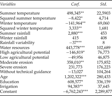
After these considerations about the determinants of irrigation adoption, we can verify the implications of adaptation in land values. However, it is first necessary to test the existence of sample selection. The estimated coefficients of ρ i are statistically equal to zero (table 3), which means that the hypothesis of the existence of sample selection bias can be rejected. In other words, while irrigation can intuitively be considered an endogenous variable (Kurukulasuriya et al., Reference Kurukulasuriya, Kala and Mendelsohn2011) and a test for sample selection is therefore desirable, this study fails to find evidence of sample selection. In this case, the OLS estimates may thus be unbiased and consistent. Accordingly, following the approach presented by Di Falco et al. (Reference Di Falco, Veronesi and Yesuf2011), we performed estimates with the simplest approach – OLS – including a dummy variable equaling 1 to indicate the use of irrigation in a county and 0 to indicate its absence. The result (Appendix, table A2) shows that there is a difference between irrigated and rainfed farms (the coefficient of the dummy variable ‘Irrigation’ is positive and statistically significant).
The hypothesis for the existence of sample selection bias was also rejected by Di Falco et al. (Reference Di Falco, Veronesi and Yesuf2011). However, as also stated by these authors, the differences in the coefficients of the land values equation between counties with irrigation and those with rainfed agriculture demonstrate the presence of heterogeneity in the sample. In other words, the land values equations (table 3, last two columns) are significantly different. Regarding the climate variables, the land value of rainfed production is affected only by rainfall (Summer Rainfall and Rainfall Variability). For the irrigated production, all climate variables were significantly different from zero. It should be emphasized that the values of the variables Summer Temperature and Squared Summer Temperature indicate an inverted U-shaped behavior. This result shows that even with adaptation, there will be damages resulting from increased temperatures at specific levels.
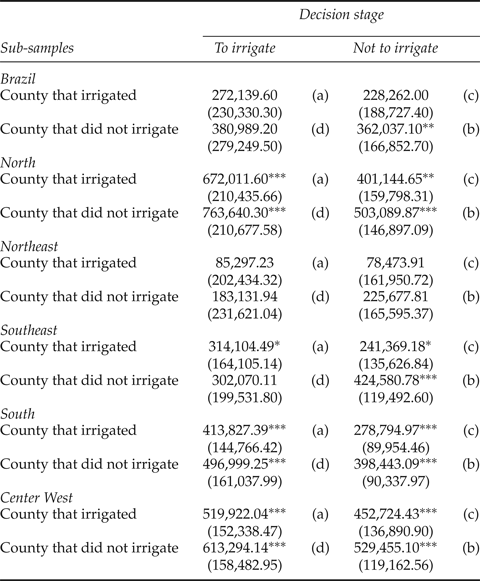
Because Brazil is a country of continental dimensions, regional differences are likely to occur in terms of climate and agro-ecological zones, agricultural production and economic development. Because of these variations, we present the expected land values under actual and counterfactual conditions aggregated for Brazil and its different geographic regions (table 4).Footnote 11
Average expected land values for regions in Brazil (R$)

Notes: Standard errors in parentheses. ***, ** and * indicate significance at the 1%, 5% and 10% levels, respectively.
Cells (a) and (b) represent the expected land value observed in the sample. It can be observed that in the Northeast, Southeast, Center West, and the aggregate result for Brazil, the land value of irrigated production tends to be lower than under rainfed production. This result is the opposite only in the North and South. We can provide two plausible explanations for this result. On the one hand, it can be stated that, while irrigation may lead to net gains and an increase in land values relative to the no-irrigation case, the gains from irrigation may not be large enough to ensure that land values in irrigated counties are higher than in dryland counties. On the other hand, this may involve the relatively lower productivity of land requiring irrigation. In many cases, irrigation has been used on lower quality soils that would not provide a dependable return under rainfed production conditions.
However, according to Di Falco et al. (Reference Di Falco, Veronesi and Yesuf2011), a simple comparison of the observed land value of irrigators and rainfed farmers (table 4) could be misleading and could lead to the conclusion that irrigation is not an effective adaptation measure in Brazil. These values should be associated with their respective counterfactual cases.
Therefore, the observed land value of irrigators (a) should be compared with estimated land value if the same farmers did not irrigate their cropland (c). In this case, considering the counties that currently irrigate, we found that if they changed to rainfed production, the land values would decrease considerably (in Brazil the net effect would be approximately −16 per cent). The reduction is higher in the North (−40 per cent). In the South and Southeast, which are regions with the largest portions of commercial agriculture in the country, reductions would be −32 and −23 per cent, respectively (table 4).
In contrast, the observed land value of rainfed farmers (b) should be compared with estimated land value if the same farmers irrigated their cropland (d). The results showed that, if there was irrigation in the counties where only rainfed agriculture is used, land values would increase. Again, the North and South regions have more significant values, with increases of 52 and 24 per cent, respectively (table 4).
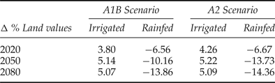
After the discussion about the current scenario, we consider the impacts of projected climate change for two representative scenarios that span the range of predictions for Brazil. We used the same previously estimated parameters to evaluate the possible benefits of irrigation as an adaptive measure as well as losses related to the decision of not adapting. The results are presented in table 5.
Impacts of climate scenarios on land values in Brazil (percentage changes in relation to the current scenario)

Note: Differences between two classes of farmers are statistically significant at less than 1% (based in standard errors calculated by bootstrap).
Following Mendelsohn et al. (Reference Mendelsohn, Nordhaus and Shaw1994) and Seo (Reference Seo2011), simulations were performed changing the climatic conditions and keeping socioeconomic and agronomic conditions unchanged. According to Seo (Reference Seo2011), it should be noted that many things other than climate will change in the future, such as technological factors, economic development, agricultural policy and international trade regimes. However, Seo (Reference Seo2011) explains that the aim of this type of simulation is to separate the effects of climate from other changes in economic conditions.
In future simulations, results show that returns associated with irrigated production are always higher than rainfed production. In the counties where agriculture is practiced using irrigation systems, the average value of land tends to increase; in the counties where agricultural production is exclusively dryland, reduction in the average value of land is substantial. It is believed that the lower magnitude of the estimated losses in our study compared with other studies of Latin America is due to different conditions regarding Brazilian agricultural infrastructure. Compared to other countries, Brazil has the most diverse and modern agriculture and therefore is more likely to take adaptive actions. From these results and analysis of studies about the impact of climate change on developing countries (Mendelsohn and Seo, Reference Mendelsohn and Seo2007; Seo and Mendelsohn Reference Seo and Mendelsohn2008a; Kurukulasuriya et al., Reference Kurukulasuriya, Kala and Mendelsohn2011; Seo, Reference Seo2011; Cunha et al., Reference Cunha, Coelho, Féres and Braga2013), it was found that irrigation can be an effective tool to counteract the harmful effects of climate change.
According to the International Panel on Climate Change (IPCC, 2007), the degree to which a locality is susceptible to the adverse effects of climate change is a function of the characteristics and magnitude of both climate variability and the locality's adaptive capacity. A high adaptive capacity reduces the potential for loss at any level of exposure to climate change. Therefore, it is expected that the Southeast and South regions and part of the Center West region will suffer fewer negative impacts because a higher probability of using irrigation was estimated for these regions. Particularly in the South, the increase in temperature could improve agricultural production in colder locations. Conversely, those regions with a lower probability of using irrigation systems will be the most affected. The Northeast region, besides suffering large increases in temperature, must also cope with reduced water availability. The expectation is that the poorest regions, characterized by family farms that are poorly capitalized, are the most vulnerable to changes in climate change. To change this situation it is important to invest in human capital (ensure greater access to information and formal education) as well as to ensure greater access to capital for investment in irrigation.
5. Conclusions
Our results confirmed prior expectations that irrigation is influenced by key climatic variables and thus should be modeled as an adaptive measure. In a general sense, the analysis of factors associated with the adoption of irrigation in Brazil showed that to be an irrigator, the farmer must have: sufficient income to afford the investment cost; technical knowledge of technology's potential, limitations, operation and functioning; and administrative abilities to manage a more capitalized farm operation. In addition to these factors, the farm must have good water availability and soil conditions appropriate for irrigated production.
It is possible to conclude that irrigators' land values tend to be more stable, demonstrating the effectiveness of irrigation as an adaptive measure. Given the predictions of climate change, irrigation has the potential to contribute to the improvement of the country's agricultural performance, making producers less vulnerable to climate. In a general sense, the results of this study reinforce the need for public policies that seek to find strategies to combat the effects of global warming in the agricultural sector. Moreover, given the evidence of the importance of irrigation as an adaptive measure, the creation of specific credit policies for the implementation of this practice should be encouraged, especially for less capitalized producers. This approach would help to address regional inequalities in credit access across the country.
The discussion about sustainability of irrigation technologies is not addressed in the study methodology and is beyond the scope of this paper. Nevertheless, it is important to mention that to maximize the potential benefits of irrigation as an adaption response, it will be necessary to make this practice more environmentally ‘clean’. Practices must be applied to ensure proper irrigation management, thus avoiding the waste of water and other problems caused by the improper use of irrigation technology. It is essential to inform producers about the proper selection of irrigation methods, which should be guided by the nature and location of production, and local field and soil characteristics.
It is also necessary to emphasize that a large-scale conversion to irrigated production across areas of the country will have significant resource impacts even under the highest levels of on-farm irrigation management. The potential impacts include producer-level effects (e.g., higher pumping costs, variability in surface water supplies as supplies become more limiting, potential increases in field salinity), off-site economic impacts of increasing water scarcity, and environmental effects (e.g., land subsidence, dewatered streams, water-quality impairment from drainage, habitat impairment). Large-scale irrigation development will require much more than on-farm technology transfer. Institutional structures would likely need to be developed to establish legal water rights (and recourse for potentially impacted parties), construct the necessary storage/conveyance infrastructure, administer the allocation of available water supplies, and provide ongoing technical assistance at the farm-level.
Several limitations of this study must be highlighted. First, it was not possible to empirically estimate the availability of future water in the model. The amount of water available for diverse consumptive uses is not fully quantified and will most likely change, which has implications for future irrigation development. Changing climate patterns may contribute to shifts in the quantity and timing of precipitation and evapotranspiration with implications for surface-water supplies and shallow groundwater reserves. Moreover, this study does not capture the full range of adjustments that could be performed. In particular, when assuming fixed portions of land, it was not possible to analyze how the patterns of land use for agricultural and non-agricultural purposes will change. Because this is a partial equilibrium analysis, the study also does not investigate the implications of these results in terms of the effects on other sectors of the economy. We suggest that future studies account for these issues and for the sustainability of irrigation technologies.
Appendix
Brazilian geographic sampled regions.

AOGCM scenarios by 2020, 2050 and 2080 (changes in relation to the current period)

Parameters for estimates of land values