





Impact statement
During coastal storms, waves and storm tides push water inland, increasing the risk to homes, roads, dunes and beaches. Knowing how high the water will reach is therefore essential for preparing for storms and planning for future sea-level rise. However, this is hard to predict, especially because there are many existing methods that can work well for some conditions but not so good elsewhere. This study improves that picture by using evidence left behind after storms, such as lines of marine debris, to estimate how far the water reached along beaches in New South Wales, Australia. These observations were then used to test different ways of predicting storm water levels. The study shows that some simple prediction methods work better than others. In particular, models based on detailed airborne laser measurements of beach slope were more accurate than those using newer satellite-based estimates. It also found that a formula developed specifically for beaches in southeast Australia performed well even during very large storms. The wider importance of this research is that it gives coastal planners and emergency managers better guidance on how to estimate storm flooding at sandy beaches. It also shows that storm impacts can be studied using practical field evidence collected after an event, even when direct measurements during the storm are difficult. As sea levels rise and coastal populations grow, better estimates of how far storm water can reach will help communities make smarter decisions about development, protection and climate adaptation.
Highlights
-
• Large regional dataset of surveyed marine debris lines following storms in south-eastern Australia shows regional and intra-beach variability in extreme total water levels (TWLs).
-
• Extreme TWL is modelled using tidal gauges, local nearshore wave data, several empirical runup formulae and beach slope specifications from LiDAR and satellites.
-
• Large variability in model accuracy occurs across different runup formulae and beach slope specifications.
-
• Beach slope uncertainty is leveraged to account for modelling errors from deterministic slopes
-
• Errors from present-day TWL modelling can exceed the magnitudes and uncertainties of projected sea level rise.
Introduction
Coastal storms can inflict widespread damage on infrastructure and the environment, posing significant threats to coastal communities and economies. Among the primary storm hazards is coastal inundation caused by elevated water levels, which can lead to flooding in low-lying areas, damage to adjacent beach infrastructure and, in extreme cases, loss of life. With increasing anthropogenic pressures on coastal areas (Neumann et al., Reference Neumann, Vafeidis, Zimmermann and Nicholls2015; Jones and O’Neill, Reference Jones and O’Neill2016), sea level rise (SLR) (Kulp and Strauss, Reference Kulp and Strauss2019; Hague et al., Reference Hague, McGregor, Murphy, Reef and Jones2020; Khojasteh et al., Reference Khojasteh, Haghani, Nicholls, Moftakhari, Sadat-Noori, Mach, Fagherazzi, Vafeidis, Barbier, Shamsipour and Glamore2023) and uncertainties regarding future trends in extreme storm events (Mentaschi et al., Reference Mentaschi, Vousdoukas, Dosio, Voukouvalas and Feyen2017; Reguero et al., Reference Reguero, Losada and Méndez2019; Meucci et al., Reference Meucci, Young, Hemer, Kirezci and Ranasinghe2020; Morim et al., Reference Morim, Vitousek, Hemer, Reguero, Erikson, Casas-Prat, Wang, Semedo, Mori, Shimura, Mentaschi and Timmermans2021; Casas-Prat et al., Reference Casas-Prat, Hemer, Dodet, Morim, Wang, Mori, Young, Erikson, Kamranzad, Kumar, Menéndez and Feng2024), the risk from elevated water levels is likely to exacerbate (Vitousek et al., Reference Vitousek, Barnard, Fletcher, Frazer, Erikson and Storlazzi2017; Taherkhani et al., Reference Taherkhani, Vitousek, Barnard, Frazer, Anderson and Fletcher2020), threatening local infrastructure along developed coastlines globally (Vousdoukas et al., Reference Vousdoukas, Mentaschi, Voukouvalas, Verlaan, Jevrejeva, Jackson and Feyen2018; Barnard et al., Reference Barnard, Erikson, Foxgrover, Hart, Limber, O’Neill, van Ormondt, Vitousek, Wood, Hayden and Jones2019a; Almar et al., Reference Almar, Ranasinghe, Bergsma, Diaz, Melet, Papa, Vousdoukas, Athanasiou, Dada, Almeida and Kestenare2021; Casas-Prat et al., Reference Casas-Prat, Hemer, Dodet, Morim, Wang, Mori, Young, Erikson, Kamranzad, Kumar, Menéndez and Feng2024). Enhancing our knowledge and predictive capabilities of coastal inundation is therefore crucial to inform future studies supporting coastal management, disaster risk reduction and adaptation strategies (Toimil et al., Reference Toimil, Losada, Álvarez-Cuesta and Le Cozannet2023, Reference Toimil, Losada, Nicholls, Dalrymple and Stive2020).
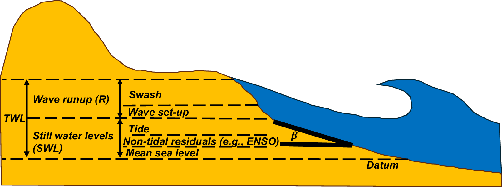
Quantifying extreme coastal water levels during storms is the baseline for coastal inundation hazard assessments. Coastal practitioners and planners rely on extreme water level predictions to identify low-lying areas vulnerable to flooding (Almar et al., Reference Almar, Ranasinghe, Bergsma, Diaz, Melet, Papa, Vousdoukas, Athanasiou, Dada, Almeida and Kestenare2021; Benito et al., Reference Benito, Aerts, Eilander, Ward and Muis2024; Chtioui et al., Reference Chtioui, Hakkou, Aangri, El Hassani, El Mostafa and Benmohammadi2024), plan future coastal developments (Mather et al., Reference Mather, Stretch and Garland2011), and estimate berm and dune erosion (Beuzen et al., Reference Beuzen, Goldstein and Splinter2019; Oliver et al., Reference Oliver, Kinsela, Doyle and McLean2024; Palmsten and Holman, Reference Palmsten and Holman2012), among other applications. Along global wave-dominated sandy coastlines characterised by narrow continental shelves (Nyberg and Howell, Reference Nyberg and Howell2016), coastal water levels are primarily influenced by wave runup and to a lesser extent by astronomical tides and non-tidal residuals (Leaman et al., Reference Leaman, Harley, Splinter, Thran, Kinsela and Turner2021). The most widely used proxy that aggregates these processes is the total water level (TWL) variable. TWL is defined as the sum of (dynamic) still water levels (SWL) comprising tides and non-tidal residuals, and wave runup (R), resulting in TWL = SWL + R (e.g., Almar et al., Reference Almar, Ranasinghe, Bergsma, Diaz, Melet, Papa, Vousdoukas, Athanasiou, Dada, Almeida and Kestenare2021; Conlin et al., Reference Conlin, Cohn and Adams2023; Zornoza-Aguado et al., Reference Zornoza-Aguado, Pérez-Díaz, Cagigal, Castanedo and Méndez2024), as illustrated in Figure 1.
A conceptual schematic highlighting the contributing factors to TWLs, including runup (swash and set-up) and still water levels (MSL, tides and non-tidal residuals), at sandy coastlines under present conditions.

Figure 1. Long description
The diagram shows a yellow sandy beach profile on the left and blue ocean water on the right. A horizontal dashed line at the bottom is labeled Datum. Moving vertically upward from the Datum, the water level is divided into two primary stacked segments.
1. The lower segment is Still water levels S W L, which is composed of three layers from bottom to top: Mean sea level, Non-tidal residuals e.g., ENSO, and Tide.
2. The upper segment is Wave runup R, which consists of two layers: Wave set-up and Swash at the top.
The combined height of S W L and R is labeled as T W L on the far left. On the right, where the water meets the shore, a black angle is labeled with the Greek letter beta, representing the beach slope. A large blue wave is shown breaking toward the shore, with the water extending up the slope of the dune to the highest point of the Swash layer.
SWL include variations from mean sea level (MSL), astronomical tides (e.g., the spring-neap cycle) and non-tidal residuals (e.g., storm surge, interannual climatic effects) (Viola et al., Reference Viola, Verdon-Kidd, Hanslow, Maddox and Power2021), typically monitored at water level stations. Alternatively, coastal practitioners use global tide models (e.g., Carrère et al., Reference Carrere, Lyard, Cancet and Guillot2015; Lyard et al., Reference Lyard, Allain, Cancet, Carrère and Picot2021) and surge models (Muis et al., Reference Muis, Aerts, Antolínez, Dullaart, Duong, Erikson, Haarsma, Apecechea, Mengel, Le Bars, O’Neill, Ranasinghe, Roberts, Verlaan, Ward and Yan2023) to estimate SWL at ungauged locations. Wave runup (R) levels – the vertical excursion of waves at the shoreline – include a time-averaged component (wave set-up) and an oscillating component of the water line (swash), commonly measured with video techniques (Holman and Stanley, Reference Holman and Stanley2007) or laser scanning (Phillips et al., Reference Phillips, Blenkinsopp, Splinter, Harley and Turner2019; Kim et al., Reference Kim, Brodie, Cohn, Giddings and Merrifield2023).
Measuring wave runup during storms is a challenging task due to the adverse weather conditions accompanying these extreme events. Video monitoring systems struggle to detect swash motions effectively under high wind and rainy conditions (Holman and Haller, Reference Holman and Haller2013; Almeida et al., Reference Almeida, Masselink, Russell and Davidson2015; Kim et al., Reference Kim, Brodie, Cohn, Giddings and Merrifield2023). In contrast, laser scanning instruments (Blenkinsopp et al., Reference Blenkinsopp, Mole, Turner and Peirson2010; Phillips et al., Reference Phillips, Blenkinsopp, Splinter, Harley and Turner2019) overcome weather/climate-related issues as they continuously measure instantaneous water levels (Almeida et al., Reference Almeida, Masselink, Russell and Davidson2015; Beuzen et al., Reference Beuzen, Goldstein and Splinter2019; Kim et al., Reference Kim, Brodie, Cohn, Giddings and Merrifield2023). However, this technology measures wave transformation only at individual cross-shore transects (Martins et al., Reference Martins, Blenkinsopp, Power, Bruder, Puleo and Bergsma2017), limiting its applicability to study extreme TWL at large scales. An alternative approach to measure extreme TWL at larger spatial scales involves surveying the position (along the beach) of the maximum elevation reached by the swash lens after a storm. Similar to other areas of coastal research (e.g., tsunami science, see for instance, Fritz et al., Reference Fritz, Petroff, Catalán, Cienfuegos, Winckler, Kalligeris, Weiss, Barrientos, Meneses, Valderas-Bermejo, Ebeling, Papadopoulos, Contreras, Almar, Dominguez and Synolakis2011), the maximum swash limit can be identified from landward marine debris deposits and/or wet/dry transitions that correspond to peak TWL during storms (Cariolet and Suanez, Reference Cariolet and Suanez2013; Suanez et al., Reference Suanez, Cancouët, Floc’h, Blaise, Ardhuin, Filipot, Cariolet and Delacourt2015). The widespread availability of real-time kinematic GPS technology (Harley et al., Reference Harley, Turner, Short and Ranasinghe2011a) enhances this method’s application for measuring extreme TWL across large scales (hundreds of km), valuable for coastal risk assessments and benchmarking of existing TWL modelling approaches (e.g., Atkinson et al., Reference Atkinson, Power, Moura, Hammond, Callaghan and Baldock2017; Gomes da Silva et al., Reference Gomes da Silva, Coco, Garnier and Klein2020).
The widespread availability of runup datasets across the Americas, Australasia and Europe has led to the development of many empirical formulae for predicting wave runup statistics (e.g., Ruggiero et al., Reference Ruggiero, Komar, Mcdougal, Marra and Beach2001; Stockdon et al., Reference Stockdon, Holman, Howd and Sallenger2006; Atkinson et al., Reference Atkinson, Power, Moura, Hammond, Callaghan and Baldock2017; Gomes da Silva et al., Reference Gomes da Silva, Coco, Garnier and Klein2020). Most of these formulae estimate R2% (i.e., the elevation exceeded by 2% of waves) based on offshore wave properties (Ho and Lo, offshore significant wave height and wave length, respectively) and a single value representative of the beach face slope (β) (Figure 1). Originally derived for planar beaches in the laboratory (Hunt, Reference Hunt1959), the ‘Hunt’ scaling relationship (R
$ \propto \tan \left(\beta \right)\sqrt{H_o{L}_o} $
 ) is typically fitted to local data characterising site-specific runup dynamics (Vousdoukas et al., Reference Vousdoukas, Wziatek and Almeida2012; Gomes da Silva et al., Reference Gomes da Silva, Coco, Garnier and Klein2020; Portch et al., Reference Portch, Cuttler, Buckley, Hansen and Lowe2023). Compared to more complex process-based models of coastal inundation (e.g., Xbeach, Roelvink et al., Reference Roelvink, Reniers, van Dongeren, van Thiel de Vries, McCall and Lescinski2009), empirical models are widely used by coastal practitioners as they can be readily applied from local to large regional scales and extrapolated to different wave and beach slope characteristics (Leaman et al., Reference Leaman, Harley, Splinter, Thran, Kinsela and Turner2021; Shope et al., Reference Shope, Erikson, Barnard, Storlazzi, Serafin, Doran, Stockdon, Reguero, Mendez, Castanedo, Cid, Cagigal and Ruggiero2022; Stockdon et al., Reference Stockdon, Long, Palmsten, Van der Westhuysen, Doran and Snell2023). Stockdon et al. (Reference Stockdon, Holman, Howd and Sallenger2006) presented a generalised R2% model derived from observations of 10 field experiments across a wide range of beach characteristics (β ranging from 0.01 to 0.11) and low to moderate wave energy (Ho ranging from 0.7 m to 2.5 m). This ‘one-model-fits-all’ formula has arguably become a standard in coastal inundation risk analysis (e.g., Vitousek et al., Reference Vitousek, Barnard, Fletcher, Frazer, Erikson and Storlazzi2017; Almar et al., Reference Almar, Ranasinghe, Bergsma, Diaz, Melet, Papa, Vousdoukas, Athanasiou, Dada, Almeida and Kestenare2021; Stockdon et al., Reference Stockdon, Long, Palmsten, Van der Westhuysen, Doran and Snell2023). In comparing their 2006 formula with a more complex process-based numerical model (Xbeach), Stockdon et al. (Reference Stockdon, Thompson, Plant and Long2014) concluded adjustments were needed for this formula to perform well under storm conditions (Ho ~ 3 m), as observed during the SandyDuck field experiment (Stockdon et al., Reference Stockdon, Holman and Survey2011). Atkinson et al. (Reference Atkinson, Power, Moura, Hammond, Callaghan and Baldock2017) tested 9 existing runup models against a blind dataset from 11 beaches in south-eastern (SE) Australia. They found that no single formula performed consistently across all 11 beaches and proposed a ‘model-of-models’ approach that fitted a Hunt-type expression to the predictions from all nine earlier models. This model-of-models was the most accurate at predicting R2% jointly with previous site-specific formulae by Vousdoukas et al. (Reference Vousdoukas, Wziatek and Almeida2012) and Holman (Reference Holman1986), although it was not tested under storm conditions (Atkinson et al., Reference Atkinson, Power, Moura, Hammond, Callaghan and Baldock2017). Recent studies have compiled larger datasets that include storm events to train machine learning models for predicting R2% (e.g., genetic programming, Gaussian models, XGBoost, Beuzen et al. Reference Beuzen, Goldstein and Splinter2019; Power et al., Reference Power, Gharabaghi, Bonakdari, Robertson, Atkinson and Baldock2019, Kim and Lee, Reference Kim and Lee2024). While these approaches perform well within their training data, their accuracy outside the training/learning range may lead to large model errors (Beuzen and Splinter, Reference Beuzen, Splinter, Jackson and Short2020; Kim and Lee, Reference Kim and Lee2024).
Despite the development of numerous site-specific and generalised runup formulae over the past decades, coastal practitioners face the daunting task of selecting the most suitable model from over 30+ options (Supplementary Appendix A in Gomes da Silva et al., Reference Gomes da Silva, Coco, Garnier and Klein2020). Moreover, adequate specification of the beach slope magnitude (β) is key in the accuracy of coastal inundation risk studies (Aucan et al., Reference Aucan, Hoeke, Storlazzi, Stopa, Wandres and Lowe2019; O’Grady et al., Reference O’Grady, McInnes, Hemer, Hoeke, Stephenson and Colberg2019) and its misspecification has been recently reported as the greatest contributor to runup modelling errors (Kim and Lee, Reference Kim and Lee2024). Nonetheless, a universal definition of β is still absent in the literature. Kim et al. (Reference Kim, Brodie, Cohn, Giddings and Merrifield2023) used laser scanning technology to test different beach slope proxies for estimating storm runup at the Duck Field Research Facility (Ho ~ 4 m). They found that pre-storm beach slope measurements can provide accurate runup estimates when compared to more complex models that consider morphological changes during storms. Unfortunately, pre-storm morphological data are often unavailable elsewhere (Simmons et al., Reference Simmons, Splinter, Harley and Turner2019; Matheen et al., Reference Matheen, Harley, Turner, Splinter, Simmons and Thran2021), forcing practitioners to rely on β values from any available (often isolated) surveys at their study sites. As illustrated in Figure 2, selecting appropriate beach slope magnitudes is essential, particularly for highly dynamic coastlines where the natural temporal variability in beach face morphology can lead to significant differences in runup estimates, often varying by several metres.
This example shows the challenges of estimating runup at dynamic beaches during storms. (a) Long-term (1976–2021) cross-shore transects at Narrabeen Beach (SE Australia) reveal large variability in beach slopes at this dynamic, intermediate beach (see inset – beach slopes were calculated between the MSL and 2 m, a proxy for the berm elevation). (b) Large variability in runup estimations during storms (Ho – 3 to 8 m, Tp = 12 s) resulting from highly variable beach slopes. Runup magnitudes were estimated using the widely adopted model of Stockdon et al. (Reference Stockdon, Holman, Howd and Sallenger2006).

Figure 2. Long description
Panel a, titled Narrabeen S E Australia Historical surveys, features a line graph with Chainage in meters on the x-axis from 0 to 150 and Elevation in meters on the y-axis from minus 2 to 10. A dashed horizontal line marks M S L at 0 meters. A thick black line represents a steep profile, while a dense cluster of thin grey lines shows the dynamic beachface between chainage 25 and 100, varying between elevation 4 and minus 1. An inset histogram shows counts on the y-axis and Beach slope beta on a logarithmic x-axis from 0.01 to 0.2. The distribution peaks around 0.1, with vertical dashed lines marking the 1 percent and 99 percent bounds.
Panel b, titled Influence of beach slope in runup estimations, plots Offshore wave height in meters from 3 to 8 on the x-axis against Runup in meters from 1.0 to 4.5 on the y-axis. A central thick black line labeled median shows a linear increase in runup from approximately 2.1 to 3.4 meters as wave height increases. This line is centered within a wide grey shaded area labeled 1-99 percent predictions from range of beach slopes. The shaded area expands as wave height increases, ranging from approximately 1.2 to 2.8 meters at an offshore wave height of 3, and from 1.9 to 4.5 meters at an offshore wave height of 8. A text box notes large variability in runup estimations for dynamic beachfaces.
The advent of remote sensing technology is revolutionising the availability of beach morphological data across extensive spatial and temporal scales (Splinter et al., Reference Splinter, Harley and Turner2018; Vitousek et al., Reference Vitousek, Buscombe, Vos, Barnard, Ritchie and Warrick2023). Episodic Airborne LiDAR flights provide topographic data at different epochs, enabling the estimation of historical beach slopes and their variability over hundreds of kilometres of coastline (Saye et al., Reference Saye, van der Wal, Pye and Blott2005; Stockdon et al., Reference Stockdon, Doran and Sallenger2009; Harley, Reference Harley, Ciavola and Coco2017). In addition, recent advances in satellite remote sensing technology now offer estimates of long-term intertidal beach slopes from local to continental scales (Vos et al., Reference Vos, Harley, Turner and Splinter2023, Reference Vos, Harley, Splinter, Walker and Turner2020, Reference Vos, Splinter, Harley, Simmons and Turner2019). These modern monitoring techniques call for a timely evaluation of these data sources to enhance modelling of extreme TWL. Such improvements are crucial for developing robust methodologies to support coastal practitioners in managing coastal flooding risks, particularly in the context of accelerating SLR.
This study utilises a novel and extensive regional dataset of extreme TWL observations collected during four storms events in New South Wales (NSW), SE Australia. These observations are sourced from regional surveys of marine debris lines representing extreme TWL. Using this detailed dataset, this work primarily addresses the question: How do observed still water levels, different runup formulae and new beach slope datasets perform in predicting TWL during storms?
After assessing the challenges associated with model and data selection, this study then explores the potential to leverage the spatio-temporal variability in beach slopes to predict a wider range of plausible TWL observations. The challenges in forward-forecasting extreme TWL under rising sea levels are also discussed.
Following a description of the TWL dataset, modelling approach and input data in Sections “Data and methods,” “Results” presents the regional scale observations and modelling results, which are discussed in the context of future coastal risk assessments in Section “Discussion.” Concluding remarks are then presented in Section “Conclusions.”
Data and methods
Study area and extreme TWL dataset
Study area: NSW – SE Australia
The study area encompasses ~330 km of coastline in NSW, SE Australia, bounded by Merewether Beach in Newcastle in the north and Shoalhaven Heads in the south (Figure 3a). The region is wave dominated (Short, Reference Short2007; Leaman et al., Reference Leaman, Harley, Splinter, Thran, Kinsela and Turner2021), characterised by energetic swells, microtides and limited surge influence due to the region’s steep and narrow continental shelf (McInnes and Hubbert, Reference McInnes and Hubbert2001). The offshore wave climate is of moderate to high energy (average Ho = 1.6 m and Tp = 9.8 s) and dominated by long-period swell waves from the SSE direction generated in the southern Tasman Sea (Short and Trenaman, Reference Short and Trenaman1992). These modal conditions are interrupted approximately 5% of the time by storm waves that exceed a significant wave height threshold of 3 m (Harley et al., Reference Harley, Turner, Short and Ranasinghe2010; Harley, Reference Harley, Ciavola and Coco2017; Lobeto et al., Reference Lobeto, Semedo, Lemos, Dastgheib, Menendez, Ranasinghe and Bidlot2024), with peaks reaching over 8 m during extreme events (Lord and Kulmar, Reference Lord and Kulmar2000). These storm waves originate from various synoptic patterns, including east coast lows that develop adjacent to the coastline (Dowdy et al., Reference Dowdy, Pepler, Di Luca, Cavicchia, Mills, Evans, Louis, McInnes and Walsh2019), mid-latitude cyclones from the south and occasionally, tropical cyclones from the northeast (Short and Trenaman, Reference Short and Trenaman1992). The region experiences a micro-tidal, semi-diurnal tide with a mean spring tide range of 1.3 m (Beuzen et al., Reference Beuzen, Goldstein and Splinter2019). Non-tidal contributions to SWL vary within ±0.4 m, influenced by surges, coastal trapped waves and multi-year climatic fluctuations (Viola et al., Reference Viola, Verdon-Kidd and Power2024, Reference Viola, Verdon-Kidd, Hanslow, Maddox and Power2021).
(a) Map of study area in SE Australia, showing the geographical distribution of marine debris surveys conducted after four storm events in October 2014, April 2015, June 2016 and July 2020. Marine debris surveys covered 37 beaches at non-truncated locations, avoiding marine debris deposits at the toe of dune scarps and seawalls. (b) Example of marine debris line and RTK-GNSS monitoring. (c) Time series of offshore wave climate and SWL forcing during all four storm events. Top to bottom panels display offshore wave properties (significant wave height, peak wave period and peak direction) and still water levels obtained from offshore wave buoys (yellow asterisks in panel a) and tide gauges (white triangles in panel a), respectively. Time series are presented for buoys and gauges located in Sydney (solid lines) and Port Kembla (dashed lines).

Figure 3. Long description
Panel a is a geographical map of the Southeast Australian coast between Newcastle and Shoalhaven. Colored dots along the coastline indicate debris surveys: purple for July 2020, green for June 2016, red for April 2015, and black for October 2014. Yellow stars mark wave buoys and white triangles mark tide gauges near Sydney and Port Kembla. A dashed yellow line indicates the 70 meter depth contour.
Panel b is a photograph showing a dense line of dark marine debris on a sandy beach. An inset photo shows a researcher using an R T K G N S S pole for monitoring.
Panel c is a grid of 16 line graphs organized by four storm events (columns) and four metrics (rows). The x-axis for all graphs is Days from storm H sub s peak, ranging from minus 1 to 3.
* Row 1: Significant wave height H sub s in meters. Peaks reach approximately 6 meters in October 2014, 8 meters in April 2015, and 6 meters in June 2016 and July 2020.
* Row 2: Peak wave period T sub p in seconds, showing fluctuations between 6 and 14 seconds.
* Row 3: Peak direction D sub p in degrees, showing shifts in wave orientation during the storms.
* Row 4: Tide gauge water level in meters A H D, showing oscillating tidal patterns between minus 0.8 and 1.2 meters.
Solid lines represent Sydney data and dotted lines represent Port Kembla data. Vertical shaded bars indicate the timing of debris line surveys.
Embayed beaches are prevalent in this region with an average length of 1.3 km and E-ESE orientation (Short, Reference Short2007; Fellowes et al., Reference Fellowes, Vila-concejo and Gallop2019) (Figure 3a). The presence of headlands at the beaches’ southern ends and prevalent SSE swells result in increasing wave energy gradients from south to north along these embayments (Harley et al., Reference Harley, Turner, Short and Ranasinghe2011b; Fellowes et al., Reference Fellowes, Vila-concejo, Gallop, Harley and Short2022; Ibaceta et al., Reference Ibaceta, Harley, Turner and Splinter2023; Ibaceta and Harley, Reference Ibaceta and Harley2024). Intermediate beach morphologies are common in this region (Wright and Short, Reference Wright and Short1984; Wright et al., Reference Wright, Short and Green1985) and typically vary from low-energy and steep sections at southern ends (low-tide terrace) to longshore bar trough, single-bar rhythmic bar-beach and transverse bar-rip states at more exposed central and northern beach sections (Doyle et al., Reference Doyle, Hesp and Woodroffe2024). The regional average intertidal beach slope is approximately 0.06 and typically varies along individual beaches due to changes in wave energy, beach state and grain size (Vos et al., Reference Vos, Deng, Harley, Turner and Splinter2022). Intermittently Closed and Open Lake or Lagoons are also prevalent in the region (Khojasteh et al., Reference Khojasteh, Rao, McSweeney, Ibaceta, Nicholls, French, Glamore, Largier, Adams, Hughes, Barry, Power, du, Tucker, Cienfuegos, Catalan and Hanslow2025).
Observations of extreme TWL
Observations of extreme TWL comprise four major meteorological events (referred to for clarity as ‘storms’) in October 2014, April 2015 (e.g., Harley et al., Reference Harley, Turner, Splinter, Phillips and Simmons2016), June 2016 (e.g., Harley, Reference Harley, Ciavola and Coco2017; Mortlock et al., Reference Mortlock, Goodwin, McAneney and Roche2017) and July 2020. Hourly offshore wave data were recorded by directional wave buoys located off Sydney and Port Kembla in approximately ~80 m water depth (Figure 3a, yellow asterisks). During these storms, the offshore significant wave height peaked between Ho = 6.0 m and Ho = 8.1 m (Figure 3c, upper panels), corresponding to annual recurrence intervals of 1–20 years (Mortlock et al., Reference Mortlock, Goodwin, McAneney and Roche2017). Hourly SWLs were measured by nearby tide gauges (Figure 3a, triangles).
Extreme TWL measurements were collected from 40 sandy embayed beaches, with 7–28 beaches surveyed per storm (solid circles in Figure 3a). Similar to Cariolet and Suanez (Reference Cariolet and Suanez2013) and Suanez et al. (Reference Suanez, Cancouët, Floc’h, Blaise, Ardhuin, Filipot, Cariolet and Delacourt2015), the methodology consisted of tracking the most landward limit between wet and dry sand, which can be easily identified by marine debris deposits immediately after the storm (Figure 3b). Measurements were conducted every ~3 m alongshore the day following the peak in Ho (Figure 3c, shaded blocks) using RTK-GPS and referenced to the local datum (GDA94 projection and vertical Australian Height Datum [AHD]). On this wave-dominated coastline, these measurements correspond to the maximum TWL during the storm (TWL = (SWL + Rmax)max), modelled from maximum hourly values of SWL and maximum run up Rmax for given wave conditions during the storm. This assumes that the debris lines were deposited not at the maximum SWL or at the maximum runup (Rmax) individually, but at the maximum combined elevation of both during the storm.
To ensure the validity of existing runup formulae, measurements were taken at non-truncated locations, avoiding marine debris deposits at the toe of dune scarps and seawalls. Over 7,000 raw TWL measurements were recorded, typically extending across hundreds of metres of beach.
Transect dataset and marine debris observations pre-processing
A pre-processing step was applied to raw marine debris observations prior to further analyses and comparison with TWL predictions. The SE Australian sandy coastline was first discretised into shore-normal transects. Planview sandy shorelines, representative of the mean high-water line, were obtained from the Smartline dataset (Hazelwood, Reference Hazelwood2009). These shorelines were used to generate a series of major shore-normal transects spaced 100 m apart alongshore, aligning with the spatial resolution of a nearshore wave transformation tool used to predict nearshore wave conditions. Raw marine debris observations located within 50 m of each major transect were averaged (i.e., 100 m alongshore-average). This window aimed to minimise the localised effects from rip currents, bore merging and three-dimensional features such as beach cusps and rip horns (e.g., Harley et al., Reference Harley, Turner, Short and Ranasinghe2011b; Harley et al., Reference Harley, Turner and Short2015). Considering four storms, a total of 471 TWL observations corresponding to 345 major transects were used for comparison with predictions. These observations were subsequently used to analyse the intra-beach and regional variability in TWLs across the four storms. The final step in pre-processing marine debris observations for model-data comparison involved scaling the TWL observations associated with R max to the equivalent elevation exceeded by 2% of the waves (i.e., R 2%), which is the statistic that most runup formulae predict. Supplementary Appendix A shows a relationship between R max and R 2% that is applied to the TWL observations prior to model-data comparison.
TWL modelling
Modelling approach and runup formulae
TWLs are modelled using TWL = SWL + R. Observations of SWL were sourced from nearby tide gauges (Figure 3c, lower panels). At this wave-dominated region, the focus is on evaluating different empirical runup formulae and specifications of beach slope to improve TWL modelling. To achieve this, seven runup models were selected based on their relevance and usage in previous coastal inundation studies in SE Australia. These included two formulae that are commonly used in coastal hazards studies in SE Australia (Shand et al., Reference Shand, Shand, Mccomb and Johnson2011), including a laboratory-based model by Hedges and Mase (Reference Hedges and Mase2004) and an older formula developed from a wide spectrum of beaches in NSW (Nielsen and Hanslow, Reference Nielsen and Hanslow1991). In addition, the model-of-models by Atkinson et al. (Reference Atkinson, Power, Moura, Hammond, Callaghan and Baldock2017), developed for SE Australian beaches during small to moderate wave conditions was considered, as well as two additional models (Holman, Reference Holman1986; Vousdoukas et al., Reference Vousdoukas, Wziatek and Almeida2012) that performed equally well against the Atkinson et al. (Reference Atkinson, Power, Moura, Hammond, Callaghan and Baldock2017) dataset. The final two models included the widely used generalised formula of Stockdon et al. (Reference Stockdon, Holman, Howd and Sallenger2006) and a recent machine learning model that comprised storm-data within their development (Power et al., Reference Power, Gharabaghi, Bonakdari, Robertson, Atkinson and Baldock2019). The mathematical expressions of these formulae are presented in Table 1.
Summary of empirical models for predicting R2% used in this study

Table 1. Long description
The table contains three columns: Authors, Empirical formula, and Description.
* Holman 1986: R sub 2 percent = 0.83 tan beta square root of H sub o L sub o + 0.2 H sub o. Description: Site-specific field formula from Duck research facility, NC, USA.
* Nielsen and Hanslow 1991: R sub 2 percent = 1.98 L sub R. Where L sub R = 0.85 tan beta square root of H sub o L sub o if tan beta is greater than or equal to 0.1; and L sub R = 0.085 square root of H sub o L sub o if tan beta is less than 0.1. Description: Regional specific field formula from SE Australia.
* Hedges and Mase 2004: R sub 2 percent = 1.49 tan beta square root of H sub o L sub o + 0.34 H sub o. Description: Laboratory formula.
* Stockdon et al. 2006: R sub 2 percent = 0.043 square root of H sub o L sub o if tan beta / square root of H sub o / L sub o is less than 0.3. Otherwise, R sub 2 percent = 1.1 open parenthesis square root of numerator H sub o L sub o open parenthesis 0.563 beta squared + 0.004 close parenthesis all over 2 + 0.35 beta square root of H sub o L sub o close parenthesis if tan beta / square root of H sub o / L sub o is greater than or equal to 0.3. Description: Generalised formula from 10 field studies.
* Vousdoukas et al. 2012: R sub 2 percent = 0.53 beta square root of H sub o L sub o + 0.58 tan beta H sub o + 0.45. Description: Site specific field formula from Algarve, Portugal.
* Atkinson et al. 2017: R sub 2 percent = 0.92 tan beta square root of H sub o L sub o + 0.16 H sub o. Description: Regional specific model applied to SE Australian field data.
* Power et al. 2019: Refers to Equation 9 in the original source. Description: Generalised machine learning formula forced by H sub o, L sub o, and d sub 50 median sand grain size.
Runup formulae are forced with offshore wave data inputs (Ho and Lo). Available wave data from offshore wave buoys (Figure 3c, upper panels) were first transformed to the 10 m contour to account for wave transformation across the continental shelf and intra-beach gradients in wave energy due to protruding headlands (Fellowes et al., Reference Fellowes, Vila-concejo, Gallop, Harley and Short2022). A model (Baird, 2017) based on the WAVEWATCHIII v4.18 model (Tolman, Reference Tolman2014) was used to simulate wave conditions at 10 m depth contour every 100 m along the coastline, commensurate with the locations of 100 m spaced major shore-normal transects (Section “Transect dataset and marine debris observations pre-processing”). This tool utilises pre-developed transformation matrices (look-up tables) covering the full range of wave periods, directions and wave heights (19×19×19 joint combinations) pertinent to SE Australia. Depending on the location of the desired wave modelling output, the tool is forced with either the Sydney or Port Kembla wave buoy data (Figure 3a). Previous evaluations of this tool showed a strong agreement (Pearson correlation coefficient, ρ ~ 0.9) with nearshore wave buoys at two beaches considered in the present study (Baird, 2017; Kinsela et al., Reference Kinsela, Morris, Ingleton, Doyle, Sutherland, Doszpot, Miller, Holtznagel, Harley and Hanslow2024). Following the recommendations by Stockdon et al. (Reference Stockdon, Holman, Howd and Sallenger2006) and Gomes da Silva et al. (Reference Gomes da Silva, Coco, Garnier and Klein2020), offshore storm data were transformed to 10 m depths and subsequently reverse-shoaled to offshore conditions (Ho, Lo) to comply with the input requirements of the selected runup formulae.
Beach slopes (β) from LiDAR and satellites
Adequate beach slope specification is critical for modelling coastal inundation hazard (e.g., Figure 2). This study leverages emerging remote-sensing technologies to derive historical beach slope magnitudes and their variability. A total of three beach slope proxies from LiDAR and satellite data were used for this purpose.
LiDAR data
Topographic data in the form of digital elevation models from multiple episodic regional scale LiDAR surveys commissioned by the NSW Government were used to estimate historical beach slope magnitudes and variability. On average, each beach was surveyed eight times (standard deviation ~3) over a 17-year period (2007–2023). Previous comparisons of LiDAR-derived topography and in situ RTK-GPS surveys in this region indicated vertical and horizontal accuracies better than 0.3 and 0.8 m, respectively (Middleton et al., Reference Middleton, Cooke, Kearney, Mumford, Mole, Nippard, Rizos, Splinter and Turner2013; Doyle and Woodroffe, Reference Doyle and Woodroffe2018). LiDAR typically covers the entire dune-beach system down to MSL (~0 m AHD). The reader is referred to Beuzen et al. (Reference Beuzen, Goldstein and Splinter2019), Doyle and Woodroffe (Reference Doyle and Woodroffe2018), Harley (Reference Harley, Ciavola and Coco2017), Linklater et al. (Reference Linklater, Morris and Hanslow2023) and Middleton et al. (Reference Middleton, Cooke, Kearney, Mumford, Mole, Nippard, Rizos, Splinter and Turner2013) for more details.
Following the discretisation of the coastline into 100 m major transects (Section “Transect dataset and marine debris observations pre-processing”), historical (i.e., long-term average) beach slopes at these locations were calculated from β distributions sampled over different LiDAR flights and 100 m alongshore windows. Similar to Doran et al. (Reference Doran, Long and Overbeck2015), an additional higher resolution 10 m spaced minor transect dataset was used to sample β over 100 m windows (i.e., 11 transects spaced every 10 m), capturing alongshore variability in β associated with beach cusps and rip horns (Harley et al., Reference Harley, Turner, Short and Ranasinghe2011b; Harley et al., Reference Harley, Turner and Short2015; Ibaceta et al., Reference Ibaceta, Harley, Turner and Splinter2023).
Individual β samples were estimated using a linear regression between fixed upper and lower elevations. Based on previous literature that specified elevations from morphological and water level proxies (e.g., dune crest, berm height, tidal planes, Doran et al., Reference Doran, Long and Overbeck2015; Stockdon et al., Reference Stockdon, Long, Palmsten, Van der Westhuysen, Doran and Snell2023; Vos et al., Reference Vos, Harley, Splinter, Walker and Turner2020), this study explores two approaches: (1) beach slopes calculated between MSL (~0 m AHD) and the MHWS (mean high water springs, 0.7 m AHD this site, Beuzen et al., Reference Beuzen, Goldstein and Splinter2019) and (2) beach slopes calculated between MSL and the berm height (e.g., Harley et al., Reference Harley, Turner and Short2015). These two proxies represent (1) the slope of the partial inter-tidal zone (hereafter MSL-MHWS) and (2) the beach steepness considering the largely subaerial beach face morphology at these intermediate beaches that would be in the swash zone at high tides (hereafter MSL-berm). The 2 m AHD contour was selected as a pragmatic estimate of the beach berm height across this region as recommended by Kinsela et al. (Reference Kinsela, Morris, Linklater and Hanslow2017).
Satellite-derived slopes
Given the limited availability of continuous high-resolution LiDAR data elsewhere, a novel satellite-derived β dataset was also tested for estimating extreme TWL. The publicly available Australian beach slope dataset presented in Vos et al. (Reference Vos, Deng, Harley, Turner and Splinter2022) was employed for this purpose. In this dataset, beach slopes were estimated using the CoastSat Toolbox (Vos et al., Reference Vos, Splinter, Harley, Simmons and Turner2019). CoastSat retrieves time series of cross-shore shoreline evolution from 30+ years (1987 onwards) of publicly available satellite imagery (Landsat 5, 7, 8 and Sentinel-2). By analysing these time series at individual shore-normal transects, the long-term partial inter-tidal beach slope (i.e., the slope between MSL and MHWS) is estimated using a frequency-domain analysis (Vos et al., Reference Vos, Harley, Splinter, Walker and Turner2020), such that an optimised β minimises high-frequency tidal variations in the satellite-derived signal. This method demonstrated strong accuracy (coefficient of determination, ρ2 ~ 0.9) between satellite-derived slopes (hereafter CoastSat) and in situ long-term averages across eight different beaches in Australia, Europe, USA and Mexico (Vos et al., Reference Vos, Harley, Splinter, Walker and Turner2020). However, slightly more scatter was observed at intermediate beach states characterised by larger temporal variability in beach slopes, compared to better performance at gently sloping profiles. The dataset provides β magnitudes every 100 m along the coastline, consistent with the resolution of the major transect dataset (Section “Transect dataset and marine debris observations pre-processing”).
Performance of TWL modelling
Hourly time series of TWL = SWL + R were modelled using observed SWL data, local nearshore wave data, seven runup formulae and three β specifications (two from LiDAR and one from CoastSat). Maximum hourly values of TWL during the storm were evaluated against 471 post-processed TWL debris lines observations collected from 40 beaches during four storms. Model accuracy was assessed using several metrics, including the coefficient of determination (ρ2), root mean square error (RMSE) and model bias (BIAS).
Results
Observations of extreme TWLs
Figure 4 illustrates the regional variability in observed extreme TWL during four storms in SE Australia, referencing data to the local Australian vertical datum (m AHD). These results summarise 100 m averaged marine debris observations, commensurate with the resolution of major transect dataset. From top to bottom, panels a–d show results across four storms (October 2014–July 2020). From left to right, TWL data (in bars) denote averages by beach, ordered from north to south (Beach #1 to #40, horizontal axes). Maxima and minima TWL along individual beaches are shown in coloured and white dots, respectively. The error bars reflect intra-beach variability, calculated as the standard deviation of TWL observations.
Regional observations of total water levels from marine debris lines recorded during four storms (panels a–d) across 37 individual beaches (ordered from north to south, horizontal axes). Horizontal dashed lines indicate the regional average marine debris elevation by storm. Bars show the intra-beach average and standard deviation (black lines). Coloured and white dots indicate the maximum and minimum measurements by beach, respectively. No bars indicate no measurement at that beach.

Figure 4. Long description
A multi-panel bar chart with four stacked horizontal panels labeled a through d. The y-axis for all panels is Observed marine debris line elevation in meters A H D, ranging from 0 to 6. The x-axis represents Beach number from 1 to 40, ordered North to South.
* Panel a (October 2014, black bars): Data is concentrated between beaches 15 and 37. Elevations mostly hover around the regional storm average of approximately 3.5 meters.
* Panel b (April 2015, red bars): Data points are scattered across the North (beaches 2 to 4), Central (beaches 9 to 18), and South (beaches 24 to 31). The regional average is higher, near 5 meters.
* Panel c (June 2016, green bars): This panel has the highest data density, with measurements for almost all beaches from 4 to 35. Most bars are near the 5-meter regional average, with a peak near beach 4 exceeding 6 meters.
* Panel d (July 2020, magenta bars): Data is sparse, appearing at beaches 2, 3, 10, 16 to 18, 20 to 22, and 25 to 31. The regional average is approximately 4 meters.
Each bar includes a black vertical error bar representing standard deviation. A white dot at the bottom of the error bar indicates the minimum measurement, and a colored dot at the top indicates the maximum measurement. Horizontal dashed lines in the background of each panel represent the regional average for that specific storm event.
Across the four storms, the June 2016 event exhibited the highest average regional TWL at 5.2 m AHD, closely followed by the April 2015 storm with an average of 5.1 m. The July 2020 event recorded a lower average TWL of 4.7 m AHD, while the October 2014 event had the lowest average of 3.7 m AHD. TWL varied along individual beaches (error bars, standard deviation) by up to 1.1 m (minimum of 0.1 m). The distinction between maximum and minimum TWL at each beach (coloured and white dots) highlights localised effects and alongshore variability, with the maximum observations exceeding the minimum by an average of 0.7 m, ranging from 0.1 to 3.2 m across the dataset. These results suggest that the observed local and regional scale variability in extreme TWLs may arise from differing magnitudes of local wave characteristics and beach morphology, which are critical factors to consider in modelling approaches.
Modelling extreme TWLs
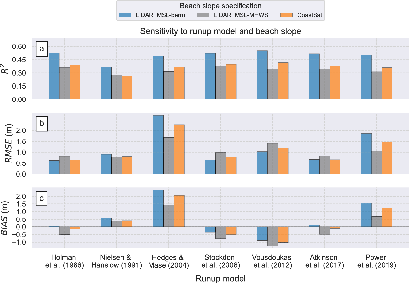
Figure 5 summarises the performance of various empirical approaches in predicting TWL, using combinations of measured SWL, local nearshore wave data, seven runup models and three beach slope specifications. Model skill was calculated for the entire dataset (471 observations) after scaling TWL to the elevation exceeded by 2% of the waves (Supplementary Appendix A, hereafter referred to as TWL for simplicity). From top to bottom, panels (a)–(c) in Figure 5 depict the coefficient of determination ρ2 (−), RMSE (in m) and BIAS (in m), respectively. The horizontal axis indicates different runup models, ordered chronologically from left to right, with coloured bars denoting different beach slope specifications. Blue and grey bars correspond to LiDAR-derived beach slopes calculated between the lower MSL and the upper berm (2 m AHD, MSL-berm, average slopes 0.08 and std. 0.02) and MHWS (0.7 m AHD, MSL-MHWS, average slopes 0.06 and std. 0.02), respectively. Orange bars show results for the CoastSat beach slopes (MSL-MHWS, average slopes 0.07 and std. 0.01).
Summary statistics of total water level modelling (TWL = SWL + R, 472 observations) for three different beach slope specifications (indicated by different colours) and seven runup formulae (displayed on horizontal axes) across all four storms. Top to bottom panels show the coefficient of determination (ρ2), root mean square error (RMSE) and BIAS. Different runup formulae are ordered chronologically from left to right.

Figure 5. Long description
A multi-panel bar chart titled Sensitivity to runup model and beach slope. A legend at the top identifies three beach slope specifications: LiDAR M S L-berm (blue), LiDAR M S L-M H W S (grey), and CoastSat (orange).
All panels share a horizontal axis labeled Runup model with seven categories ordered chronologically: Holman et al. 1986, Nielsen and Hanslow 1991, Hedges and Mase 2004, Stockdon et al. 2006, Vousdoukas et al. 2012, Atkinson et al. 2017, and Power et al. 2019.
Panel a: Vertical axis is R super 2 ranging from 0.00 to 0.60. Blue bars consistently show the highest correlation, peaking near 0.55 for Vousdoukas et al. 2012. Grey and orange bars are lower, generally between 0.25 and 0.40.
Panel b: Vertical axis is R M S E in meters ranging from 0.0 to 2.0. Hedges and Mase 2004 and Power et al. 2019 show the highest error, with blue bars exceeding 1.5 meters. Other models maintain R M S E below 1.0 meter.
Panel c: Vertical axis is B I A S in meters ranging from -1.0 to 2.0. A horizontal zero line indicates neutral bias. Hedges and Mase 2004 and Power et al. 2019 show strong positive bias (overestimation), while Stockdon et al. 2006 and Vousdoukas et al. 2012 show negative bias (underestimation) across all slope types.
Figure 5a reveals that using beach slopes between the MSL and the berm (MSL-berm, blue bars) explained up to 57% of the TWL variability (ρ2 = 0.57, Vousdoukas et al., Reference Vousdoukas, Wziatek and Almeida2012 model), and on average, 51% of variability across all models. Model skill decreases for β calculated in the partial intertidal zone (MSL-MHWS) and CoastSat (ρ2 = 0.36 and 0.38 across all models, respectively). The differences in model performance using different beach slope specifications were less remarkable in terms of RMSE (Figure 5b) and BIAS (Figure 5c), although variability across different runup formulae was notable (horizontal axes). RMSE values were generally lower than 1 m, with the models by Holman (Reference Holman1986), Stockdon et al. (Reference Stockdon, Holman, Howd and Sallenger2006) and Atkinson et al. (Reference Atkinson, Power, Moura, Hammond, Callaghan and Baldock2017) achieving the lowest errors (~0.6 m). Conversely, the formulae by Hedges and Mase (Reference Hedges and Mase2004) and Power et al. (Reference Power, Gharabaghi, Bonakdari, Robertson, Atkinson and Baldock2019) exhibited lower performance (RMSE >1.1 m and up to 2.7 m). As for the BIAS metric (Figure 5c, BIAS = predicted – observed), Hedges and Mase (Reference Hedges and Mase2004) and Power et al. (Reference Power, Gharabaghi, Bonakdari, Robertson, Atkinson and Baldock2019) models showed considerable overestimation, up to 2.5 and 1.6 m, respectively. Modelling TWL using other formulae resulted in both over-and-underestimations of less than ~1 m. Notably, the models by Atkinson et al. (Reference Atkinson, Power, Moura, Hammond, Callaghan and Baldock2017) and Holman (Reference Holman1986) demonstrated the lowest BIAS (|BIAS| < 0.4 m) across all beach slope specifications.
To explore the results in further detail, representative scatter plots of modelled and observed TWL are presented in Figure 6 for a mix of laboratory, site specific, generalised and machine learning runup formulae. Left to right panels indicate different β specifications (from left to right, LiDAR MSL-berm, LiDAR MSL-MHWS and CoastSat). Top to bottom panels indicate different runup formulae, including a laboratory-based model (Hedges and Mase, Reference Hedges and Mase2004), the widely used and generalised model by Stockdon et al. (Reference Stockdon, Holman, Howd and Sallenger2006), the SE Australian model-of-models by Atkinson et al. (Reference Atkinson, Power, Moura, Hammond, Callaghan and Baldock2017) and a recent machine learning model by Power et al. (Reference Power, Gharabaghi, Bonakdari, Robertson, Atkinson and Baldock2019). Additional scatter plots for the remaining three models used in the present study can be found in Supplementary Appendix B. Black dashed lines indicate a 1:1 line (perfect fit), while continuous coloured lines indicate the modelled linear fit to assist with the interpretation of results.
Example scatter plots of total water level modelling (TWL = SWL + R, 471 observations) for three different beach slope specifications (represented by different colours from left to right) and four runup formulae (displayed from top to bottom panels). Each dot indicates an individual observation and its corresponding modelled value. The black dashed lines present a perfect fit (1:1). Coloured solid lines are linear fits obtained from the modelled data and are included to facilitate the interpretation of the model’s skill and performance.

Figure 6. Long description
A grid of twelve scatter plots arranged in four rows and three columns.
Axes and Legend:
* The horizontal x-axis represents Observed extreme total water levels in meters A H D, ranging from 1 to 6.
* The vertical y-axis represents Modelled extreme total water levels in meters A H D, ranging from 1 to 11.
* A top legend identifies three data series: blue dots for L i D A R M S L-berm slopes, grey dots for L i D A R M S L-M H W S slopes, and orange dots for CoastSat slopes.
* A black dashed line in every plot represents a 1 to 1 perfect fit.
* Solid colored lines represent the linear fit for each dataset.
Row-by-Row Breakdown:
* Row 1 (Hedges and Mase 2004): Panels a, b, and c. Data points are clustered above the 1 to 1 line, showing a significant overestimation of water levels. The linear fit lines have steep positive slopes.
* Row 2 (Stockdon et al. 2006): Panels d, e, and f. Data points are clustered below the 1 to 1 line, indicating an underestimation. The linear fit lines have a shallower slope compared to the first row.
* Row 3 (Atkinson et al. 2017): Panels g, h, and i. Data points are more closely aligned with the 1 to 1 dashed line, showing improved model accuracy, though some underestimation persists at higher values.
* Row 4 (Power et al. 2019): Panels j, k, and l. Similar to the first row, these plots show an overestimation, with data points and solid linear fit lines positioned above the dashed 1 to 1 line.
The scatter plots show varying degrees of model performance, with individual errors ranging from ~1 m and up to 2–3 m. The Hedges and Mase (Reference Hedges and Mase2004) and Power et al. (Reference Power, Gharabaghi, Bonakdari, Robertson, Atkinson and Baldock2019) (Figure 6a–c, j–l) tend to overpredict TWL across all beach slope specifications, as indicated by their linear fits lying above the 1:1 line. In contrast, the models by Stockdon et al. (Reference Stockdon, Holman, Howd and Sallenger2006) (Figure 6d–f) and Atkinson et al. (Reference Atkinson, Power, Moura, Hammond, Callaghan and Baldock2017) (Figure 6g–i) provide predictions closer to the 1:1 line. This is particularly true for the combination of MSL-berm slopes (blue dots) and the Atkinson et al. (Reference Atkinson, Power, Moura, Hammond, Callaghan and Baldock2017) formula (Figure 6g, ρ2 = 0.55, RMSE = 0.6 m, BIAS = 0.1 m) that resulted in superior predictions over the entire range of TWL values including extremes (e.g., TWL > 4 m AHD). In contrast, predictions using the Stockdon et al. (Reference Stockdon, Holman, Howd and Sallenger2006) formula were less evenly distributed around the 1:1 line and underpredicted TWL extremes (Figure 6d). Underprediction of extreme TWL is also apparent for β specifications in the partial intertidal zone (MSL-MHWS) and CoastSat (Figure 6e,f,h,i), suggesting that considering as much of the entire beach face as practical (MSL-berm) is critical for predicting extreme TWL during storms.
Discussion
Modelling extreme TWLs
Application of runup formulae to TWL modelling
Coastal practitioners often face the challenge of selecting from numerous existing (30+) and emerging runup formulae for coastal inundation risk assessments. Comparing 471 TWL observations with models using gauged SWL and seven runup formulae resulted in varying degrees of model performance (Figure 5). The most accurate models were the SE Australia-specific Atkinson et al. (Reference Atkinson, Power, Moura, Hammond, Callaghan and Baldock2017) and Holman (Reference Holman1986), achieving the lowest RMSE (~0.6 m and minimal average errors (|BIAS| < 0.4 m) across all beach slope specifications. Although the Holman (Reference Holman1986) formula was calibrated with data from the Duck Research Facility (USA), Atkinson et al. (Reference Atkinson, Power, Moura, Hammond, Callaghan and Baldock2017) attributed their comparable performance to an identical mathematical structure and similar magnitudes in their model’s free-parameters (see Table 1). It is plausible that the strong performance of the Holman (Reference Holman1986) model reflects similarities between the intermediate beach states typical of SE Australia and those observed at Duck.
Notably, this study demonstrated that the most accurate model, Atkinson et al. (Reference Atkinson, Power, Moura, Hammond, Callaghan and Baldock2017), which was developed during small to moderate conditions (Ho ~ 1.5 m in their study), can be extrapolated to extreme conditions (Ho ~ 6 to 8.1 m in this study) without loss of performance. This result is relevant since accurate TWL predictions during extreme storms are likely the most important to coastal practitioners in identifying low-lying areas subjected to coastal flooding (Almar et al., Reference Almar, Ranasinghe, Bergsma, Diaz, Melet, Papa, Vousdoukas, Athanasiou, Dada, Almeida and Kestenare2021). The feasibility of transferring other formulae to predict extreme conditions elsewhere requires further validation.
Modelling TWL using other runup models formulated elsewhere (e.g., Holman, Reference Holman1986; Stockdon et al., Reference Stockdon, Holman, Howd and Sallenger2006; Vousdoukas et al., Reference Vousdoukas, Wziatek and Almeida2012) resulted in RMSE errors of ~1 m (Figure 5b), except for the laboratory-based models (Hedges and Mase, Reference Hedges and Mase2004) and machine learning applications (Power et al., Reference Power, Gharabaghi, Bonakdari, Robertson, Atkinson and Baldock2019), which exhibited higher errors (RMSE = 1.1–2.7 m) and overestimated TWL by up to 2.5 m (Figure 5c). These results are consistent with previous research indicating that laboratory-derived formulae tend to underperform when applied to field-data (Atkinson et al., Reference Atkinson, Power, Moura, Hammond, Callaghan and Baldock2017) and ‘generalised’ machine learning approaches can produce significant errors when used outside their learning/training range (Goldstein et al., Reference Goldstein, Coco and Plant2019; Beuzen and Splinter, Reference Beuzen, Splinter, Jackson and Short2020; Gomes da Silva et al., Reference Gomes da Silva, Coco, Garnier and Klein2020; Kim and Lee, Reference Kim and Lee2024). The widely adopted formula by Stockdon et al. (Reference Stockdon, Holman, Howd and Sallenger2006) consistently underestimated TWL (BIAS approximately −0.5 m across all beach slope specifications), particularly at the most relevant higher levels (e.g., TWL > 4 m, Figure 6d–f). Consistent with previous studies (Vousdoukas et al., Reference Vousdoukas, Wziatek and Almeida2012; Stockdon et al., Reference Stockdon, Thompson, Plant and Long2014; Atkinson et al., Reference Atkinson, Power, Moura, Hammond, Callaghan and Baldock2017), systematic errors in generalised ‘one-model-fits-all’ parameterisations, such as Stockdon et al. (Reference Stockdon, Holman, Howd and Sallenger2006), can lead to inaccuracies when applied to other sites. Novel approaches that tailor machine-learning model architectures to varying hydrodynamic and beach-state conditions (e.g., Itzkin et al., Reference Itzkin, Palmsten, Buckley, Birchler and Torres-Garcia2025) provide a more suitable solution than generalised, one-model-fits-all frameworks.
Importantly, this study demonstrated that for the wave-dominated SE Australian coastline, models previously calibrated for similar morphodynamic characteristics (Atkinson et al., Reference Atkinson, Power, Moura, Hammond, Callaghan and Baldock2017) performed better (including during extreme storms) than generalised, emergent machine learning and laboratory-based approaches. These results imply that coastal practitioners are recommended to increasingly utilise site-specific formulae in their coastal risk assessments. Depending on project/management objectives, first-pass assessments of coastal inundation risk employing appropriate TWL modelling approaches can be complemented by more advanced process-based modelling methodologies (e.g., Barnard et al., Reference Barnard, Erikson, Foxgrover, Hart, Limber, O’Neill, van Ormondt, Vitousek, Wood, Hayden and Jones2019b; Zornoza-Aguado et al., Reference Zornoza-Aguado, Pérez-Díaz, Cagigal, Castanedo and Méndez2024). The success of these methodologies will only be achieved if data collection efforts during storms (Kim et al., Reference Kim, Brodie, Cohn, Giddings and Merrifield2023) continue to support runup benchmarking studies (e.g., Atkinson et al., Reference Atkinson, Power, Moura, Hammond, Callaghan and Baldock2017; Gomes da Silva et al., Reference Gomes da Silva, Coco, Garnier and Klein2020).
Sensitivity of beach slope specifications to TWL modelling
Defining appropriate beach slope specifications (β) is crucial for coastal inundation risk assessments (e.g., Figure 2, Aucan et al., Reference Aucan, Hoeke, Storlazzi, Stopa, Wandres and Lowe2019; Kim et al., Reference Kim, Brodie, Cohn, Giddings and Merrifield2023; Kim and Lee, Reference Kim and Lee2024). To assist coastal practitioners in SE Australia with a fit-for-purpose quantification of this key parameter, our study tested three time-invariant historical beach slope specifications from emerging remote sensing technologies. TWL predictions using long-term LiDAR slopes calculated between the MSL and berm height (ρ 2 = 0.51 across all models) outperformed those using slopes calculated in the partial intertidal zone (LiDAR, MSL-MHWS) and satellite-derived CoastSat slopes, which also represent the MSL-MHWS, by approximately 15% (ρ2 = 0.36 and 0.38, respectively, Figure 5a).
LiDAR-derived slopes are better (or at least similarly well) suited for coastal inundation risk assessments than satellite-derived approaches for storm conditions in this coastline. Comparable skill between LiDAR MSL-MHWS and CoastSat slopes is not surprising, as the latter are also a proxy of the partial intertidal zone (MSL-MHWS) (Vos et al., Reference Vos, Deng, Harley, Turner and Splinter2022, Reference Vos, Harley, Splinter, Walker and Turner2020). Both MSL-MHWS specifications showed underestimation of TWL extremes (Figure 6h,i), highlighting the importance of using as much of the beach face as practical (MSL-berm) for predicting extreme TWL during storms in intermediate-state beaches common in SE Australia (Wright and Short, Reference Wright and Short1984). These results highlight the importance of using a broader portion of the beach face (here, the MSL–berm zone) to estimate TWL under storm conditions, rather than relying on narrower segments (e.g., only part of the intertidal zone) that may be more suitable for calmer conditions.
To our knowledge, this study is the first published attempt to implement and evaluate satellite-derived slopes into large-scale TWL modelling. Although these slopes resulted in lower (or similar) skill than higher resolution LiDAR slopes, they remain a valuable resource for data-poor regions lacking continuous coastal monitoring programs using more costly techniques (Splinter et al., Reference Splinter, Harley and Turner2018; Vitousek et al., Reference Vitousek, Buscombe, Vos, Barnard, Ritchie and Warrick2023). The emergence of enhanced higher-resolution satellite-derived techniques (e.g., CubeSats, Doherty et al., Reference Doherty, Harley, Vos and Splinter2022) will potentially result in improved quantifications of satellite-derived coastal morphological variables from local to global scales (e.g., Pronk et al., Reference Pronk, Hooijer, Eilander, Haag, de Jong, Vousdoukas, Vernimmen, Ledoux and Eleveld2024) and pave the way for enhanced local to global coastal inundation risk assessments in view of accelerating SLR.
Challenges and opportunities for coastal inundation risk studies
Leveraging beach slope uncertainty for TWL modelling
Despite decades of research on runup modelling, there remains no perfect predictive runup model for coastal inundation risk studies. As demonstrated in this study, even the best performing formulae and beach slope specifications can lead to scatter and large individual errors of several metres (e.g., Figure 5b). Instead of solely aiming to reduce these errors in deterministic models (e.g., Kim and Lee, Reference Kim and Lee2024), emerging and growing research on probabilistic predictions offers a more comprehensive approach to coastal hazard modelling by predicting a range of possible outcomes (Kinsela et al., Reference Kinsela, Morris, Linklater and Hanslow2017; Limber et al., Reference Limber, Barnard, Vitousek and Erikson2018; Beuzen et al., Reference Beuzen, Goldstein and Splinter2019; Vitousek et al., Reference Vitousek, Cagigal, Montaño, Rueda, Mendez, Coco and Barnard2021). Essentially, probabilistic outputs provide likelihoods of TWL which are generally required for risk assessments by coastal management and planning frameworks.
To enhance TWL forecasting performance, we explored a straightforward probabilistic, data-driven approach that leverages the uncertainty inherent in available beach slope data, disregarding other sources of uncertainty that cannot be quantified for this study (e.g., nearshore wave transformation). Considering that average beach slopes were calculated from several LiDAR flights centred at 100 m spaced major transects (e.g., Doran et al., Reference Doran, Long and Overbeck2015, Section “Transect dataset and marine debris observations pre-processing”), the β range can be used to estimate a wider range of TWL outcomes (e.g., Figure 2). Doran et al. (Reference Doran, Long and Overbeck2015) defined the concept of mean residual error, MRE (i.e., the standard deviation of β at each transect) and used it to estimate lower and upper beach slope ranges (95% C.I., Mean ± 1.96MRE, here shown in Figure 7a for MSL-berm slopes). By repeating the TWL modelling process with these upper (green) and lower (red) β bounds, a range of TWL predictions were obtained that account for beach slope variability (Figure 7b). This straightforward analysis, previously applied in Stockdon et al. (Reference Stockdon, Long, Palmsten, Van der Westhuysen, Doran and Snell2023), considers the variability in beach slope, as the only single source of uncertainty and shows that the range of TWL predictions (between green and red linear regressions) encompass the majority of the model errors in deterministic models from average beach slopes (blue dots) for this coastline. This assessment demonstrates the potential to leverage the uncertainty of this key input variable (β) as a source of uncertainty for TWL modelling, giving practitioners a simple means to quantify uncertainty without incorporating less-understood errors from sources such as formulas, wave transformation or wave-parameter estimates.
Influence of varying beach slope ranges on predicting the highly variable observed total water levels. (a) Lower, mean and upper range distributions of beach slopes derived from spatio-temporal LiDAR data. While the above analyses considered the regional distribution of averaged beach slopes across each transect (central boxplot in panel a), an updated analysis considering beach slope uncertainty accounts for the majority of observed range in total water levels (panel b).

Figure 7. Long description
Panel a is a boxplot titled Beach slope distributions L i D A R M S L-berm. The y-axis is Beach slope beta ranging from 0.00 to 0.20. The x-axis has three categories. First, Lower range Mean minus 1.96 M R E shown as a red box with a median near 0.02. Second, Mean shown as a blue box with a median near 0.08. Third, Upper range Mean plus 1.96 M R E shown as a green box with a median near 0.13.
Panel b is a scatter plot titled Atkinson et al. 2017. The x-axis is Observed T W L in meters A H D ranging from 2 to 6. The y-axis is Modelled T W L in meters A H D ranging from 1 to 8. Blue data points are scattered around a central dashed black 1 to 1 line. A thick blue line represents the linear fit. A large grey shaded region, bounded by a green line at the top and a red line at the bottom, represents predictions from the range of beach slopes shown in panel a. The grey region encompasses the vast majority of the observed data points.
By implementing probabilistic TWL modelling approaches, coastal practitioners will be able to provide more comprehensive assessments of coastal flooding considering a complete range of potential modelling outcomes now and into the future.
Implications for future coastal inundation hazard and risk assessments
TWL forecasts are crucial to identify areas of coastline that may experience coastal flooding in coming decades. Under the well-established assumption of minor (5%–10%) projected changes in global waves (Morim et al., Reference Morim, Hemer, Wang, Cartwright, Trenham, Semedo, Young, Bricheno, Camus, Casas-Prat, Erikson, Mentaschi, Mori, Shimura, Timmermans, Aarnes, Breivik, Behrens, Dobrynin, Menendez, Staneva, Wehner, Wolf, Kamranzad, Webb, Stopa and Andutta2019; Casas-Prat et al., Reference Casas-Prat, Hemer, Dodet, Morim, Wang, Mori, Young, Erikson, Kamranzad, Kumar, Menéndez and Feng2024), future open-coast inundation assessments typically incorporate magnitudes of SLR directly into TWL models (Vitousek et al., Reference Vitousek, Barnard, Fletcher, Frazer, Erikson and Storlazzi2017; Almar et al., Reference Almar, Ranasinghe, Bergsma, Diaz, Melet, Papa, Vousdoukas, Athanasiou, Dada, Almeida and Kestenare2021). SLR projections vary based on different time horizons, climate change and emission scenarios, currently known as Shared Socioeconomic Pathways (SSPs).
Given the observed errors in current TWL predictions (e.g., Figure 5a), it is worthwhile to compare these with the uncertainties in future SLR projections (e.g., Wahl et al., Reference Wahl, Haigh, Nicholls, Arns, Dangendorf, Hinkel and Slangen2017; Agulles and Jordà, Reference Agulles and Jordà2024). Figure 8 shows the TWL modelling errors (RMSE) from different runup formulae with the median and likely range (17%–83%) projected SLR for 2050 and 2100 in Sydney (SE Australia), using the latest data from the Intergovernmental Panel on Climate Change Sixth Assessment Report (IPCC, 2023; Kopp et al., Reference Kopp, Garner, Hermans, Jha, Kumar, Reedy, Slangen, Turilli, Edwards, Gregory, Koubbe, Levermann, Merzky, Nowicki, Palmer and Smith2023). This analysis reveals that the uncertainties in present-day TWL modelling can exceed both the magnitudes and uncertainties of projected SLR across the broad spectrum of plausible scenarios (i.e., SSP126 to SSP585 scenarios, horizontal lines and shaded areas in Figure 8). This result highlights the need for improved TWL modelling and the incorporation of uncertainty across all constituents of the modelling framework (e.g., Figure 7). As the distributions of future sea level uncertainty up to 2150 and across different pathways become more accessible through publicly available resources (e.g., the NASA sea level projection tool, e.g., Garner et al., Reference Garner, Hermans, Kopp, Slangen, Edwards, Levermann, Nowicki, Palmer, Smith, Fox-Kemper, Hewitt, Xiao, Aðalgeirsdóttir, Drijfhout, Golledge, Hemer, Krinner, Mix, Notz, Nurhati, Ruiz, Sallée, Yu, Hua, Palmer and Pearson2022, https://sealevel.nasa.gov/ipcc-ar6-sea-level-projection-tool), there is a significant opportunity to enhance the assessments of future open-coast inundation risks. With global coastal policies increasingly mandating the incorporation of climate change in future coastal planning (Thom, Reference Thom2022), coastal practitioners will need to incorporate uncertainty across the entire modelling framework, including rising sea levels, potential changes in waves (Morim et al., Reference Morim, Wahl, Vitousek, Santamaria-Aguilar, Young and Hemer2023) and storm surges (Muis et al., Reference Muis, Aerts, Antolínez, Dullaart, Duong, Erikson, Haarsma, Apecechea, Mengel, Le Bars, O’Neill, Ranasinghe, Roberts, Verlaan, Ward and Yan2023). Until we gain more holistic knowledge on these future drivers of coastal change, related planning decisions should be made with caution.
Implications for future coastal inundation risk studies. Comparison of the TWL modelling skill (RMSE) for different formulae and projected sea level rise magnitudes in SE Australia by 2050 and 2100 under SSP126 and SSP585 scenarios.

Figure 8. Long description
The X-axis is labeled Runup formula and lists seven specific models: Holman 1986, Nielsen & Hanslow 1991, Hedges & Mase 2004, Stockdon et al. 2006, Vousdoukas et al. 2012, Atkinson et al. 2017, and Power et al. 2019. The Y-axis is labeled R M S E (bars) and S L R projection (lines) in meters, ranging from 0.0 to 2.5.
Four horizontal lines represent S L R projections:
* S S P 1 2 6-2050: Dashed blue line at approximately 0.15 meters.
* S S P 5 8 5-2050: Dashed black line at approximately 0.2 meters.
* S S P 1 2 6-2100: Solid blue line at approximately 0.35 meters.
* S S P 5 8 5-2100: Solid black line at approximately 0.75 meters.
Shaded regions indicate the likely range for these projections, with a light blue band for 2050 scenarios and a light gray band for 2100 scenarios.
Vertical blue bars represent the R M S E for each formula:
* Holman: ~0.6 meters.
* Nielsen & Hanslow: ~0.9 meters.
* Hedges & Mase: ~2.7 meters (the highest error).
* Stockdon et al.: ~0.65 meters.
* Vousdoukas et al.: ~1.0 meter.
* Atkinson et al.: ~0.65 meters.
* Power et al.: ~1.85 meters.
Text in the upper right quadrant states: Errors from present day T W L modelling can exceed magnitudes of projected sea level rise.
Conclusions
Coastal practitioners increasingly require accurate predictions of extreme TWL in order to implement appropriate disaster risk measures and effectively prepare for coastal flooding events. This study has presented a novel, comprehensive and large-scale dataset of extreme TWL observations collected during four storms in SE Australia. Following the description of this dataset, this study performed a comprehensive analysis on the performance of different runup formulae and beach slope specifications in predicting observed TWL.
Analysis of 471 TWL observations from these storms revealed considerable intra-beach and regional variability in TWL. By comparing these observations with TWL models derived from gauged SWL, local nearshore wave transformation tools, seven runup formulae and three beach slope specifications from remote-sensing techniques, varying runup modelling performances were observed. TWL predictions using historical beach slopes from LiDAR data outperformed (~15% increase in model skill) the models using emerging satellite-derived slopes, although the latter are still deemed a reasonable/valuable source for data-poor regions. Results indicated varying model performances across different runup formulae and identified the best performance for a model previously developed in SE Australia under moderate wave conditions (Atkinson et al., Reference Atkinson, Power, Moura, Hammond, Callaghan and Baldock2017, ρ2 = 0.55, RMSE = 0.6 m, BIAS = 0.4 m). This highlights the effectiveness of using site-specific tailored models over more generic, widely adopted ‘one-model-fits-all’ approaches and emergent machine learning formulae. Furthermore, this study demonstrated that existing models typically calibrated during small to moderate wave conditions can be reliably extrapolated to extreme storm events, provided they are applied to sites of similar morphodynamic characteristics.
Our analyses showed that uncertainty in beach slope measurements could account for a large portion of the observed model errors, highlighting the potential to leverage the inherent uncertainty of this variable as a single major source of uncertainty in present-time TWL modelling. Overall, this work presented the value of emerging TWL datasets collected during storms and provided a robust framework to assist coastal practitioners in enhancing forward forecasting applications. By leveraging both site-specific models and uncertainty in key model input variables, coastal risk assessments can be improved, leading to better preparedness and response strategies in the face of increasingly extreme coastal events.
Open peer review
To view the open peer review materials for this article, please visit http://doi.org/10.1017/cft.2026.10043.
Supplementary material
The supplementary material for this article can be found at http://doi.org/10.1017/cft.2026.10043.
Data availability statement
Transect data are available at https://datasets.seed.nsw.gov.au/dataset/nsw-open-coast-inundation-from-wave-overtopping-2025.
Acknowledgements
Offshore wave data were collected by the Manly Hydraulics Laboratory on behalf of the NSW Department of Climate Change, Energy, the Environment and Water (DCCEEW). We thank Baird Australia for providing the nearshore wave transformation matrices. Tom Doyle, Kym Bilham and Tracey MacDonald (DCCEEW) are acknowledged for their feedback on the first iteration of this manuscript. We also thank the sea level projection authors for developing and making the sea-level rise projections available, multiple funding agencies for supporting the development of the projections and the NASA Sea Level Change Team for developing and hosting the IPCC AR6 Sea Level Projection Tool.
Author contribution
Conceptualisation: R.I., D.H.; Data curation: B.M., D.H.; Funding acquisition: D.H.; Formal analyses: R.I., M.H.; Project administration: R.I., D.H., D.K.; Methodology: R.I., B.M., D.H.; Software: R.I.; Validation: R.I.; Visualisation: R.I.; Writing – original draft: R.I., M.H., D.K., D.H.; Writing – review and editing: R.I., M.H., D.K., D.H.
Funding statement
Funding for this work was provided by the NSW Climate Change Fund and the NSW DRRF Fund which is jointly funded by the Australian and New South Wales (NSW) governments. Raimundo Ibaceta was funded by the NSW Climate Change Adaptation Strategy.




 Open access


Comments
Dear Editors:
On behalf of my co-authors and myself, I am pleased to submit the following manuscript titled “Challenges and opportunities in predicting coastal total water levels from empirical runup models: Insights from major storms in Southeast Australia
” for consideration for publication in Cambridge Prisms.
Coastal storms pose significant threats to infrastructure, ecosystems, and communities, causing widespread flooding and damage. Quantifying extreme coastal water levels during storms is essential for coastal inundation risk assessments, and effective planning and management practices. Total water levels (TWL) - the combination of wave runup, tides, and surges – and in the future, sea level rise, remain the most critical variable driving open-coast flooding during such extreme events. However, despite decades of research, a fundamental challenge for coastal practitioners is selecting from numerous (30+) existing and increasingly emerging runup models, often constrained by unavailable site-specific beach slope data.
This study addresses these challenges by presenting a novel, regional-scale dataset of extreme TWL observations, derived from marine debris deposits surveyed immediately after four major storms in New South Wales, Southeast Australia. Using this dataset, we assess the accuracy of traditional coastal flooding models by integrating gauged still water levels, local nearshore wave data, various runup formulae, and beach steepness estimates obtained from emerging remote sensing technologies. Our findings reveal significant variability in model performance, with better results when using LiDAR-derived beach slopes compared to emerging satellite-derived slopes. Notably, a formula developed specifically for Southeast Australia outperformed more widely used one-model-fits-all approaches. We also demonstrate that considering the local variability in beach slope through probabilistic outputs can account for the majority of errors obtained from deterministic approaches, with important implications for global flood predictions in the context of uncertain sea level rise.
Our study provides a valuable framework to assist coastal practitioners with forecasting applications in view of climate change, highlighting the need to address TWL uncertainties in order to fully assess potential flooding impacts. We expect wide interest across different disciplines, from coastal engineers/managers to climate change experts.
I look forward to hearing from you. Please contact me at your convenience should you require any additional information. Thank you in advance for your time and consideration.
Best regards,
Raimundo Ibaceta