







1. Introduction
Internal solitary waves (ISWs) are large amplitude nonlinear waves, with a vertical structure that displaces isopycnals either purely downwards (waves of depression) or purely upwards (waves of elevation). They are common features of stratified lakes, estuaries and the coastal ocean (Helfrich & Melville Reference Helfrich and Melville2006; Lamb Reference Lamb2014; Boegman & Stastna Reference Boegman and Stastna2019). These waves transport energy away from their generation sites over long distances. As they approach the coast, they interact with the bottom boundary layer (BBL), which is the region of the water column where the ISWs are affected by the presence of the seafloor (Trowbridge & Lentz Reference Trowbridge and Lentz2018). The BBL extracts energy and momentum from the waves, often in the form of turbulent eddies, which provide a mechanism for energy dissipation and the transport of mass, heat and momentum vertically in the water column. These fluxes have implications for basin-scale energy budgets, circulation and water quality.
Although the BBL is characteristically forced by external flows (e.g. tides and surface waves), strongly nonlinear ISWs have the potential to impose unsteady and non-negligible horizontal pressure gradients that lead to rapid acceleration/deceleration of the flow (Zulberti, Jones & Ivey Reference Zulberti, Jones and Ivey2020). The ISW induces a horizontal current, which is maximum beneath the wave trough (figure 1a). This streamwise velocity distribution imposes both favourable and adverse pressure gradients on the BBL under the front and rear shoulders of the ISW, respectively. If the adverse pressure gradient is sufficiently large, the boundary layer can separate (figure 1b–d). Upstream of the separation point, the flow will reverse near the bed, forming a shear layer with an inflectional velocity profile (figure 1b,c).
(a) Vorticity field and velocity vectors of a typical rightward-propagating ISW. The black thick line indicates the pycnocline location. Triangles on the  $x$-axis of panel (a) mark the location of the near-bed velocity profiles shown in panels (b–h) at
 $x_w/L_w -0.75$,
 $-0.5$,
 $-0.25$, 0, 0.25, 0.5 and 0.75, respectively.

This profile supports the amplification of small perturbations and is susceptible to an absolute instability (Huerre & Monkewitz Reference Huerre and Monkewitz1990). If the local absolute instability has a sufficient streamwise length scale, global instability can occur (Huerre & Monkewitz Reference Huerre and Monkewitz1990). The instability is said to be global, rather than local, due to the non-parallel streamwise dependence of the base flow. The signature of this global mechanism is the continuous excitation of self-sustained instabilities that grow and trigger vortex shedding that trails the ISW (e.g. Diamessis & Redekopp Reference Diamessis and Redekopp2006; Sakai, Diamessis & Jacobs Reference Sakai, Diamessis and Jacobs2020). This contrasts with a so-called convective instability that would fall behind the ISW. In the field (Bogucki & Redekopp Reference Bogucki and Redekopp1999; Johnson, Weidemann & Pegau Reference Johnson, Weidemann and Pegau2001; Bogucki, Redekopp & Barth Reference Bogucki, Redekopp and Barth2005) and in the laboratory (Aghsaee & Boegman Reference Aghsaee and Boegman2015; Ghassemi, Zahedi & Boegman Reference Ghassemi, Zahedi and Boegman2022), localized sediment resuspension has been observed under the rear shoulder of the ISW. The resuspension has often been attributed to a global instability of the separated region.
The production of unstable vortices by global instability of the separated BBL, beneath ISWs, was first suggested by Bogucki & Redekopp (Reference Bogucki and Redekopp1999) and then supported by laboratory (Carr, Davies & Shivaram Reference Carr, Davies and Shivaram2008; Zahedi, Aghsaee & Boegman Reference Zahedi, Aghsaee and Boegman2021) and numerical (e.g. Diamessis & Redekopp Reference Diamessis and Redekopp2006; Aghsaee et al. Reference Aghsaee, Boegman, Diamessis and Lamb2012; Sakai et al. Reference Sakai, Diamessis and Jacobs2020) experiments. This is the commonly discussed instability mechanism resulting from the interaction of ISWs and the BBL (Bogucki & Redekopp Reference Bogucki and Redekopp1999; Bogucki et al. Reference Bogucki, Redekopp and Barth2005; Carr et al. Reference Carr, Davies and Shivaram2008; Boegman & Stastna Reference Boegman and Stastna2019; Zahedi et al. Reference Zahedi, Aghsaee and Boegman2021; Zulberti et al. Reference Zulberti, Jones and Ivey2020). However, as stated by Boegman & Stastna (Reference Boegman and Stastna2019), the possibility of global instability is somewhat surprising given that the stratified shear instabilities, described in linear theory (i.e. by the Taylor–Goldstein equation), have propagation speeds that are much lower than the long wave speed. The long wave speed, in turn, provides a strict lower bound on the ISW propagation speed. In fact, Zulberti et al. (Reference Zulberti, Jones and Ivey2020) did not observe a global instability in their measurements of ISWs on the Australian continental shelf.
Verschaeve & Pedersen (Reference Verschaeve and Pedersen2014) challenged the global instability paradigm by solving the parabolized stability equations for the linear instability of the spatially varying flow under an ISW. They concluded that the BBL under an ISW behaves as a noise amplifier, suggesting that the primary linear instability is convective. They showed steeper amplification of instabilities with increasing  $Re$ and suggested that background seed noise, in both laboratory and numerical domains, is critical to trigger flow instability. These different interpretations of flow instability indicate that the nature of the BBL instability beneath an ISW, in response to changes in Reynolds number, requires further investigation.
Laboratory experiments of lock–release-generated ISWs (Carr & Davies Reference Carr and Davies2006; Carr et al. Reference Carr, Davies and Shivaram2008; Zahedi et al. Reference Zahedi, Aghsaee and Boegman2021) agree on a threshold for vortex shedding,  $Re_{ISW}\approx 200$,
 $P_{ISW}\approx 0.05\unicode{x2013}0.07$, defined in 2.2. This observed threshold is much lower than the threshold computed from two-dimensional (2-D) spectral direct numerical simulations (DNS) initialized with an ISW waveform (Diamessis & Redekopp Reference Diamessis and Redekopp2006; Aghsaee et al. Reference Aghsaee, Boegman, Diamessis and Lamb2012) (see figure 5(b) in Zahedi et al. (Reference Zahedi, Aghsaee and Boegman2021)). However, other 2-D numerical models can reproduce relevant features of the BBL beneath lock–release-generated ISWs in the laboratory. For example, numerical simulations by Thiem et al. (Reference Thiem, Carr, Berntsen and Davies2011) reproduced the laminar reverse velocity jet and BBL thickness of an ISW of depression initialized by lock–release in the laboratory by Carr & Davies (Reference Carr and Davies2006). More recently, 2-D finite-volume DNS by Ellevold & Grue (Reference Ellevold and Grue2023) showed good agreement in predicting the instability threshold, in comparison with the Carr et al. (Reference Carr, Davies and Shivaram2008) lock–release experiments. Ellevold & Grue (Reference Ellevold and Grue2023) showed that pycnocline depth is an additional parameter relevant to parameterizing BBL stability. This raises the question as to why the ISW waveform-initialized spectral 2-D DNS do not reproduce the BBL instability threshold determined for lock–release-generated ISWs in the laboratory and confirmed with finite-volume 2-D DNS. The reasons for the lack of agreement remain unclear but may be related to differences in the background seed noise across settings (e.g. from differences in the initial conditions, bottom and sidewall friction and/or the truncation error of the numerical schemes). This argument is theoretically supported by the potential that the BBL instability is convective in nature, based on the recent evidence of noise-amplifier behaviour (Verschaeve & Pedersen Reference Verschaeve and Pedersen2014) as discussed above.
The field observations by Zulberti et al. (Reference Zulberti, Jones and Ivey2020) on the Australian continental shelf, and by Quaresma et al. (Reference Quaresma, Vitorino, Oliveira and da Silva2007) on the Portuguese shelf, reported maximum near-bed sediment concentrations, associated with maximum turbulence intensity, immediately beneath the troughs of ISWs of depression (where the flow was expected to relaminarize). This contrasts with measurements on the California inner continental shelf, where local near-bed sediment concentrations were observed to peak at the trailing edge of ISWs of depression propagating shoreward (e.g. Johnson et al. Reference Johnson, Weidemann and Pegau2001; Becherer et al. Reference Becherer, Moum, Colosi, Lerczak and McSweeney2020). This also contrasts with laboratory experiments (Aghsaee & Boegman Reference Aghsaee and Boegman2015; Zahedi et al. Reference Zahedi, Aghsaee and Boegman2021) and laboratory-scale numerical simulations (Diamessis & Redekopp Reference Diamessis and Redekopp2006; Aghsaee et al. Reference Aghsaee, Boegman, Diamessis and Lamb2012; Sakai et al. Reference Sakai, Diamessis and Jacobs2020), showing the vortex shedding and sediment resuspension to occur in the separated BBL beneath the rear shoulder of the ISW (Boegman & Stastna Reference Boegman and Stastna2019). It remains a challenge to reconcile the field observations, relative to each other and to the laboratory-scale investigations.
Overall, these discrepancies open questions regarding the nature of the BBL instability and the relevance of comparing results obtained from numerical, experimental and field-based studies. Therefore, the objectives of the present study are to investigate the convective versus absolute/global nature of the BBL instability in response to changes in Reynolds number and the sensitivity of the instability to antecedent seed noise in front of the ISW. We simulated periodic trains of ISWs, which allowed us to include the effects of remnant seed perturbations, from the wakes of preceding waves, on the ISW-induced BBL instability of subsequent waves. Through this approach, we determined the sensitivity of the BBL to external perturbations, which is a characteristic feature of convectively unstable flows. This contrasts with past numerical (e.g. Diamessis & Redekopp Reference Diamessis and Redekopp2006; Aghsaee et al. Reference Aghsaee, Boegman, Diamessis and Lamb2012; Ellevold & Grue Reference Ellevold and Grue2023) and laboratory (e.g. Carr et al. Reference Carr, Davies and Shivaram2008; Aghsaee & Boegman Reference Aghsaee and Boegman2015; Zahedi et al. Reference Zahedi, Aghsaee and Boegman2021) studies that always considered laminar conditions preceding the passage of a lone ISW. We focused on the initial development of the instability, for which 2-D DNS is suitable (e.g. Diamessis & Redekopp Reference Diamessis and Redekopp2006; Aghsaee et al. Reference Aghsaee, Boegman, Diamessis and Lamb2012; Ellevold & Grue Reference Ellevold and Grue2023) and invoked classical hydrodynamic stability theory (Drazin & Reid Reference Drazin and Reid1981).
2. Theoretical background
2.1. Linear convective, absolute and global instability
To provide the necessary theoretical framework to classify flow stability depending on its qualitative features, we briefly review the relevant theory on convective, absolute and global instability. Further detail can be found in Huerre & Monkewitz (Reference Huerre and Monkewitz1990), Schmid & Henningson (Reference Schmid and Henningson2001) and Chomaz (Reference Chomaz2005).
The classical model for a steady parallel shear flow (independent of the streamwise direction) to transition from laminar to turbulent begins with an infinitesimal localized perturbation evolving over time and space. If the flow is unstable, the amplitude of the perturbation will grow. A complete description depends on the competition between the rate of advection of energy associated with the instability (relative to the background flow) versus the local rate of growth (amplification) of the instability. If advection dominates, the growing instability is swept away from the location where it was introduced; it is a convective instability. If the growing instability spreads locally, both upstream and downstream from the source – it is an absolute instability.
In many 2-D flows, like the BBL beneath ISWs, the background velocity field is non-uniform in the streamwise direction. In this case, the stability analysis requires consideration of the streamwise coordinate as an eigendirection, and the 2-D instability of the entire flow field is termed a global instability. Global modes have a coherent structure over a finite 2-D region of the flow, such as the entire spatial extent of a separation bubble (Hammond & Redekopp Reference Hammond and Redekopp1998; Theofilis Reference Theofilis2011). In many cases, however, when the base flow varies slowly over a typical instability wavelength (i.e. weakly non-parallel flow), the notions described above for local convective and absolute instability of parallel flows, can still be applied locally at each streamwise position of the weakly non-parallel flow. In this way, it has been established that a necessary condition for the existence of a global mode, in a weakly non-parallel flow, is the presence of a sufficiently large pocket of local absolute instability (Huerre & Monkewitz Reference Huerre and Monkewitz1990). This connection is key as it allows us to investigate the nature of weakly non-parallel flows through local stability analysis at different streamwise locations in the domain (e.g. Rist & Maucher Reference Rist and Maucher2002; Marxen et al. Reference Marxen, Lang, Rist and Wagner2003; Diwan & Ramesh Reference Diwan and Ramesh2012). Within the parameter space of the present study, we will consider the BBL beneath ISWs as a weakly non-parallel flow, suitable for local stability analysis, as we argue in 5.1.
In a convectively unstable flow, the stability is highly sensitive to the amplitude and spectral content of external perturbations that are advected through the flow – these are noise amplifiers. In this case, whether an instability grows to an observable level and triggers vortex shedding and/or transition to turbulence will depend on the initial amplitude of the perturbation, which in turn depends on the initial noise level. As environmental noise is often different across different experimental, numerical and field settings, the definition of a general threshold for instability is challenging (e.g. Verschaeve & Pedersen Reference Verschaeve and Pedersen2014). Rather, the absolute/global dynamics are intrinsic, spontaneous and independent of the external noise (e.g. Huerre & Monkewitz Reference Huerre and Monkewitz1990). Global modes act as self-excited wavemaker oscillators, where instabilities are spontaneously and continuously generated, hence the evolution of vortices does not rely on the spatial amplification of external perturbations, but rather on the growth of initial disturbances in time (Huerre & Monkewitz Reference Huerre and Monkewitz1990). It is, therefore, expected that global stability threshold parameterizations be equally valid in laboratory and numerical domains.
2.2. Vortex shedding thresholds under ISWs
By reanalysing the laboratory data from Carr et al. (Reference Carr, Davies and Shivaram2008), Aghsaee et al. (Reference Aghsaee, Boegman, Diamessis and Lamb2012) argued that the BBL instability under an ISW of depression was determined by the non-dimensional pressure gradient ( $P_{ISW}$) and the momentum thickness Reynolds number (
 $Re_{ISW}$) at the separation point under the wave (figure 2). The subsequent laboratory experiments by Aghsaee & Boegman (Reference Aghsaee and Boegman2015), as analysed by Zahedi et al. (Reference Zahedi, Aghsaee and Boegman2021), supported these findings. The relevant parameters are defined as
 \begin{gather} P_{ISW}= \left ( U_2+c \right ) \frac{U_2}{L_w{g}'}, \end{gather}
 \begin{gather}Re_{ISW}= U_2 \sqrt{\frac{L_w}{\nu\left ( U_2+c \right )}} . \end{gather}
Here,  $U_2$ is the absolute value of the maximum horizontal velocity at the wave trough,
 ${g}'=g\Delta \rho /\rho _0$ is the reduced gravity,
 $\nu$ is the kinematic viscosity and
 $L_w$ is the horizontal wavelength scale (Michallet & Ivey Reference Michallet and Ivey1999),
 \begin{equation} L_w=\frac{1}{a}\int_{-\infty}^{\infty}\eta_p(x)\,{{\rm d}\kern0.06em x}, \end{equation}
where  $\eta _p(x)$ is the vertical displacement of the pycnocline. At the field scale, typical values of
 $Re_{ISW}\gtrapprox 1200\unicode{x2013}3500$ have been reported (Aghsaee et al. Reference Aghsaee, Boegman, Diamessis and Lamb2012). In the
 $Re_{ISW}$ versus
 $P_{ISW}$ space, the lock–release laboratory experiments (Carr et al. Reference Carr, Davies and Shivaram2008; Zahedi et al. Reference Zahedi, Aghsaee and Boegman2021) agree on the threshold (
 $Re_{ISW}\approx 200$,
 $P_{ISW}\approx 0.05\unicode{x2013}0.07$), which is much lower than that predicted by waveform-initialized 2-D spectral DNS (figure 2a). More recently, Ellevold & Grue (Reference Ellevold and Grue2023) conducted 2-D lock–release DNS to reproduce the laboratory experiments by Carr et al. (Reference Carr, Davies and Shivaram2008). They found that, in addition to
 $a/H$ and
 $Re_w=c_0H/\nu$, the pycnocline depth (
 $d$) is also a relevant parameter for BBL stability. They defined a critical threshold of the form
 $a/H=a_0(Re_w/Re_{w_{0}})^{-m_1}$ (figure 2b), where parameters
 $a_0$ and
 $m_1$ depend on the relative depth of the pycnocline (
 $d/H$). Here,
 $H$ is the total water depth and
 $c_0$ is the linear wave phase speed. Each threshold curve was determined from their numerical simulations to fit a selected pair of stable and unstable experiments of Carr et al. (Reference Carr, Davies and Shivaram2008) as highlighted in figure 2(b). In figure 2(b) we also include the instability threshold proposed by Diamessis & Redekopp (Reference Diamessis and Redekopp2006) based on numerical simulations of Korteweg-de Vries (KdV) solitary waves.
Stability diagrams in (a)  $Re_{ISW}$ versus
 $P_{ISW}$ space and (b)
 $a/H$ versus
 $Re_w$ space, showing our simulated cases (stars), the laboratory observations by Zahedi et al. (Reference Zahedi, Aghsaee and Boegman2021) (Z21) (circles) and Carr et al. (Reference Carr, Davies and Shivaram2008) (C08) (triangles), and the unstable ISW numerically simulated by Sakai et al. (Reference Sakai, Diamessis and Jacobs2020) (S20) (blue square). Black solid lines are stability curves from 2-D DNS by (a) Aghsaee et al. (Reference Aghsaee, Boegman, Diamessis and Lamb2012) (A12) and (b) Diamessis & Redekopp (Reference Diamessis and Redekopp2006) (D06) for a KdV wave. Blue and red lines are stability curves from 2-D DNS by Ellevold & Grue (Reference Ellevold and Grue2023) (E23) for two different pycnocline depths (
 $d/H$). Blue and red markers are the associated laboratory experiments in Carr et al. (Reference Carr, Davies and Shivaram2008) selected by Ellevold & Grue (Reference Ellevold and Grue2023) to fit each stability curve. The C08, Z21 and E23 ISWs were generated by lock release, whereas the D06, A12, S20 and present study ISWs were generated by solution of the KdV (D06) or DJL equations.

3. Methods
3.1. Problem definition
We performed spectral DNS of periodic ISWs of depression propagating over a flat bottom. We evaluated the effects of Reynolds number ( $Re_{ISW}$) on the type of BBL instability: stable, convective or absolute/global. For each
 $Re_{ISW}$, we modified the length of the periodic domain (
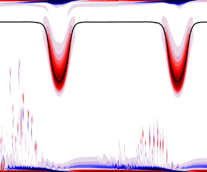
 $L_{\tau }$) to generate different decay time scales of the vortex wakes between two consecutive ISWs. A schematic of the problem is shown in figure 3, which illustrates the characteristic vortex shedding dynamics for the three different
 $Re_{ISW}$ regimes investigated. Depending on
 $Re_{ISW}$, subsequent periodic ISWs will encounter different characteristic trailing wakes from preceding ISWs: a stable laminar BBL at lower
 $Re_{ISW}$ (figure 3a), an unstable wave packet with decaying vortices at intermediate
 $Re_{ISW}$ (figure 3b) or an energetic vortex wake at higher
 $Re_{ISW}$ (figure 3c). The intensity of the wake preceding each subsequent ISW will differ, depending on the domain periodicity (i.e. more energetic for shorter
 $L_{\tau }$).
Schematic of the research problem. Vorticity field of rightward propagating periodic ISWs at different  $Re_{ISW}$. The black line represents the centre of the pycnocline. Vertical dashed lines indicate the lateral limits of the periodic domain of length
 $L_{\tau }$.

The periodic ISWs propagated along a quasi-two-layer density stratification defined via a hyperbolic tangent profile, widely used in numerical studies,
 \begin{equation} \bar{\rho}(z)=\rho_0+\Delta\rho \tanh\left( \frac{z-z_{pyc}}{h_{pyc}}\right ), \end{equation}
where  $\rho _0=1000\ {\rm kg}\ {\rm m}^{-3}$ is a reference density and
 $\Delta \rho$ is the density jump across a pycnocline of half-thickness
 $h_{pyc}=2H/35$ centred at depth
 $z_{pyc}=4H/35$ and
 $\Delta \rho /\rho _0=120/1000$, with
 $z$ positive upwards.
The ISWs were initialized using a solution of the Dubreil–Jacotin–Long (DJL) equation,
 \begin{gather} \nabla^2\eta+\frac{N^2(z-\eta)}{c^2}\eta =0, \end{gather}
 \begin{gather}\eta=0\quad \hbox{at}\ z=0,-H, \end{gather}
 \begin{gather}\eta=0\quad \hbox{as}\ x\rightarrow \pm\infty , \end{gather}
where  $\eta (x,z)$ is the vertical isopycnal displacement in the frame of reference of the wave,
 $c$ is the ISW phase speed and
 $N$ is the Brunt–Väisälä frequency defined as
 \begin{equation} N^2(z)=\frac{1}{\rho_0}\frac{{\rm d}\bar{\rho}(z)}{{\rm d}z}. \end{equation}
The DJL equation was solved numerically using the algorithm of Turkington, Eydeland & Wang (Reference Turkington, Eydeland and Wang1991) implemented by Dunphy, Subich & Stastna (Reference Dunphy, Subich and Stastna2011). We chose a wave amplitude  $a=0.37H$ with
 $L_w=2.5H$. The modelled periodic wave was a large amplitude ISW, similar to that of Sakai et al. (Reference Sakai, Diamessis and Jacobs2020), and was selected to sustain its waveform over long propagation distances.
3.2. Parameter space
We explored four  $Re_{ISW}$ regimes (figure 2a): (A) laminar
 $Re_{ISW}=90$; (B) marginally unstable, typical of laboratory-scale experiments
 $Re_{ISW}=300$; and highly unstable (C)
 $Re_{ISW}=900$, and (D)
 $Re_{ISW}=1800$, comparable to geophysical conditions. Our simulation cases were chosen based on the parameterization by Aghsaee et al. (Reference Aghsaee, Boegman, Diamessis and Lamb2012), because our simulated stability threshold was consistent with theirs, which was also from 2-D spectral DNS (not shown). These Reynolds numbers were selected in order to cover a wide range.
To provide context,  $Re_{ISW}=300$ is characteristic of an ISW with
 $a\approx 0.17$ m and
 $L_w\approx 1$ m propagating along a quasi-two-layered stratification with
 $\Delta \rho = 120\ {\rm kg}\ {\rm m}^{-3}$, and
 $z_{pyc}=0.057$ m in a laboratory flume with total depth
 $H=0.5$ m. These conditions are of similar scale to the laboratory experiments by Carr et al. (Reference Carr, Davies and Shivaram2008) and Zahedi et al. (Reference Zahedi, Aghsaee and Boegman2021). In comparison,
 $Re_{ISW}=900$ and
 $Re_{ISW}=1800$ are characteristic of ISWs with
 $a\approx 8$ and 12 m and
 $L_w\approx 60$ and 74 m, respectively, propagating along a quasi-two-layered stratification with
 $\Delta \rho =1\ {\rm kg}\ {\rm m}^{-3}$, and
 $z_{pyc}=5$ m in a lake or coastal ocean with total depth
 $H=40$ m. These conditions are similar to observations on the inner continental shelf of California (e.g. Johnson et al. Reference Johnson, Weidemann and Pegau2001; Becherer et al. Reference Becherer, Moum, Colosi, Lerczak and McSweeney2020), Cayuga Lake (Dorostkar, Boegman & Pollard Reference Dorostkar, Boegman and Pollard2017), the St. Lawrence River estuary (Bourgault et al. Reference Bourgault, Morsilli, Richards, Neumeier and Kelley2014) and the Knight Inlet fjord (Farmer & Armi Reference Farmer and Armi1999). On the outer continental shelf, the wave characteristics may be an order of magnitude larger.
We modified the viscosity to set each target  $Re_{ISW}$ (via (2.2)) – all waves propagated on the same stratification and thus had the same DJL wave properties, with constant
 $P_{ISW}=0.116$,
 $a/H=0.37$ and
 $d/H=0.11$.
For  $Re_{ISW}$ A, B and C, we simulated periodic domain lengths
 $L_\tau$, which varied between
 $L_\tau =3L_{w}$ and
 $L_\tau =12L_{w}$. The shortest ISW spacing was the limiting case and was just large enough, with respect to the ISW wavelength, to prevent any spurious interactions between the leading and trailing edges of each wave (ISW wavelength
 $\lambda _{ISW}\sim 2L_w$). The largest spacing was four times the shortest case, large enough to demonstrate the effect of varying vortex wake intensities, but limited by the required numerical resolution. For the largest
 $Re_{ISW}$ case (D), we only simulated a single wave with period
 $\tau$ to be a reference for the large
 $Re$ limit. Table 1 summarizes the simulation parameters.
Simulation parameters for each case. The domain length  $L_\tau$ was a multiple of the wavelength scale
 $L_w$. The period of each ISW train was
 $\tau = L_\tau /c$. Simulation time (
 $tc/L_{\tau }=t/\tau$) is reported as the number of periodic ISW passages through the domain. In all cases,
 $P_{ISW}=0.116$,
 $a/H=0.37$ and
 $d/H=0.11$. The total wall-clock time was
 ${\approx }30$ days, running on 64 cores of the high-performance computing clusters of Compute Ontario.

This parametric study focused on the effects of changing: (i) the laboratory to geophysical scale Reynolds number and (ii) the magnitude of antecedent seed noise, on the nature of the BBL instability. We did not seek to parameterize the stability threshold, which varies depending on methodology (figure 2). Hence, the conclusions drawn here are valid regardless of the applicable instability threshold parameterization.
3.3. Numerical simulations
We numerically solved the 2-D incompressible Navier–Stokes equations under the Boussinesq approximation,
 \begin{gather} \frac{\partial{u}}{\partial{t}} + u\frac{\partial{u}}{\partial{x}} + w\frac{\partial{u}}{\partial{z}}={-}\frac{1}{\rho_0}\frac{\partial{p}}{\partial{x}}+\nu \nabla^2 u, \end{gather}
 \begin{gather}\frac{\partial{w}}{\partial{t}} + u\frac{\partial{w}}{\partial{x}} + w\frac{\partial{w}}{\partial{z}}={-}\frac{1}{\rho_0}\frac{\partial{p}}{\partial{z}}+\nu \nabla^2 w-\frac{\rho g}{\rho_0}, \end{gather}
 \begin{gather}\frac{\partial{\rho}}{\partial{t}} + u\frac{\partial{\rho}}{\partial{x}} + w\frac{\partial{\rho}}{\partial{z}}=\kappa \nabla^2\rho, \end{gather}
 \begin{gather}\frac{\partial{u}}{\partial{x}} + \frac{\partial{w}}{\partial{z}} = 0 , \end{gather}
where  $(x,z)$ are the horizontal and vertical coordinate directions,
 $(u,w)$ are the associated velocity vectors,
 $t$ is time,
 $p$ is pressure,
 $\rho$ is the fluid density and
 $\kappa$ is the molecular diffusivity. For all cases, the simulated
 $Pr=\nu /\kappa =1$, however, we investigated various ratios between
 $\nu$ and
 $\kappa$ (1 to 10), and the results (not shown) were insensitive to changes in
 $\kappa$, since the BBL was largely neutrally stratified.
The 2-D DNS were conducted with the pseudospectral code SPINS (Subich, Lamb & Stastna Reference Subich, Lamb and Stastna2013). Recent studies have shown the ability of SPINS to solve nonlinear internal wave problems at laboratory scales to investigate wave–boundary interaction (Deepwell et al. Reference Deepwell, Clarry, Subich and Stastna2021; Hartharn-Evans et al. Reference Hartharn-Evans, Carr, Stastna and Davies2022) and boundary layer instability (Harnanan, Stastna & Soontiens Reference Harnanan, Stastna and Soontiens2017).
The computational domain was rectangular with depth  $H$ and length
 $L_\tau$, the latter varied between cases to simulate different ISW periods with different decay time scales of the vortex wake between two consecutive ISWs. To simulate the periodic passage of ISWs, the horizontal domain was periodic. The initial condition was given by the DJL solution with the ISW located in the middle of the domain (see 3.1). No-slip and no-flux boundary conditions were imposed on the top and bottom boundaries. A Chebyshev grid was employed in the vertical direction with grid points clustered near the top and bottom walls. A uniform grid was used in the horizontal direction. Grid resolutions ranged from
 $512 \times 256$ to
 $8192 \times 2048$ (table 1). Grid-halving simulations verified grid independence at these resolutions. Time-dependent simulations were completed on the high-performance computing clusters of Compute Ontario. While we had originally planned three-dimensional (3-D) simulations, it was computationally prohibitive to resolve the Kolmogorov scales, in 3-D simulations, for our set-ups using the available computational resources. However, 2-D simulations were sufficient to describe the essential dynamics of the primary instability and determine its convective versus absolute nature, invoking classical hydrodynamic stability theory (Drazin & Reid Reference Drazin and Reid1981; Verschaeve & Pedersen Reference Verschaeve and Pedersen2014).
3.4. Description of the BBL instability
To describe the evolution of the instability, we separated base ( $U$) and perturbation (
 $\hat {u}$) flow fields through low-pass and high-pass filtering of the instantaneous velocity field in wavenumber space. The cutoff wavenumber was determined from a wavelet analysis (Torrence & Compo Reference Torrence and Compo1998), which was also used to characterize the instability. We computed the evolution of wavelet spectra in the
 $k$–
 $x$ space of the vertically integrated near-bed horizontal velocity, which allowed us to track the position and wavenumber energy distribution of an unstable wave as it moved and grew with time. Here, we refer to the localized perturbation velocities, induced by the ISW-generated BBL instability, as an instability-generated wave packet. By computing the wavelet spectra in
 $k$–
 $x$ space, we tracked wave energy packets to determine if the nature of the instability was convective or absolute.
To understand the mechanisms for instability growth and their interaction with subsequent periodic ISWs, we computed the Reynolds–Orr energy budget (Schmid & Henningson Reference Schmid and Henningson2001),
 \begin{gather} \frac{{\rm D}E_v}{{\rm D}t}={-}\hat{\mathcal{P}} - \hat{\varepsilon}, \end{gather}
 \begin{gather}\hat{\mathcal{P}} = \int_{V} \hat{u}_i \hat{u}_j\frac{\partial U_i}{\partial x_j} {\rm d}V, \end{gather}
 \begin{gather}\hat{\varepsilon} = \frac{1}{Re}\int_{V}\left ( \frac{\partial \hat{u}_i}{\partial x_j} \right )^2 \,{\rm d}V, \end{gather}
which describes the rate of change of the instability kinetic energy ( $E_v=\frac {1}{2}\int _V\hat {u}_i\hat {u}_i \,{\rm d}V$) due to its interaction with the base flow
 $U_i(x,z)$ (
 $-\hat {\mathcal {P}}$) and its viscous dissipation (
 $-\hat {\varepsilon }$) over the volume
 $V$. In two dimensions,
 \begin{equation} \hat{\mathcal{P}}=\int_{V} \left( \underbrace{\hat{u} \hat{u}\frac{\partial U}{\partial x} }_{\mathcal{P}_{uu}} + \underbrace{\hat{w} \hat{w}\frac{\partial W}{\partial z}}_{\mathcal{P}_{ww}} + \underbrace{\hat{u} \hat{w}\frac{\partial U}{\partial z} }_{\mathcal{P}_{uw}} + \underbrace{\hat{w} \hat{u}\frac{\partial W}{\partial x} }_{\mathcal{P}_{wu}} \right){\rm d}V. \end{equation}
As we are interested in the near-bed region, we computed this integral over a subregion of the domain. We integrated horizontally over  $L_{\tau }$ and vertically between
 $z=0$ and
 $z=h$, where
 $h$ was large enough to encompass the instability-generated wave packet, such that
 $E_v$ fluxes through the boundaries of
 $V$ were minimized. The separation of length scales between the ISW (
 $L_w$) and the instability-generated wave packet was large enough (
 $10^2\unicode{x2013}10^3$) that the visualized unstable oscillations (
 $\hat {u}$) and the budget (3.10) were not sensitive to the choice of filtering scales within
 $\approx$10 %–20 % above and below the cutoff value.
4. Results
4.1. Vorticity field over the parameter space
The kinetic energy produced from the BBL depends upon both  $Re_{ISW}$ and
 $L_{\tau }$. This is illustrated with the vorticity field (figure 4, supplementary movies 1–10 available at https://doi.org/10.1017/jfm.2024.506). In all cases, the pycnocline was stable and ISWs propagated rightward while remaining roughly unchanged over several wave periods
 $\tau$, except for a gradual reduction in wave amplitude due to friction. Behind each wave, the BBL separated due to the adverse pressure gradient under the wave. This formed two contiguous parallel vortex sheets of opposite sign (at the bottom of figure 4a i). Under the front shoulder of each propagating ISW, the flow accelerated leftwards leading to a compression of the boundary layer.
(a,c,e) Snapshots and (b,d,f) near-bottom time-depth contours of the vorticity field for (a,b)  $Re_{ISW}=90$, (c,d)
 $Re_{ISW}=300$ and (e,f)
 $Re_{ISW}=900$. Snapshots are in the wave reference frame, with
 $x_w=0$ corresponding to the ISW trough. The time of the snapshots in panels (a,c,e) is indicated by a vertical dashed line in panels (b,d,f), respectively. Subpanels (i)–(iv) correspond to increasing
 $L_{\tau }$ for each
 $Re_{ISW}$. In all panels, the continuous black line indicates the position of the pycnocline, whose scale reads on the left-hand axis of panel (a). The axes label of panels (b,d,f) reads on the right-hand axis of panel (f). Corresponding movies of the vorticity field for simulations associated with panels (a i,b i), (a iv,b iv), (c i,d i), (c ii,d ii), (c iii,d iii), (c iv,d iv), (e i,f i), (e ii,f ii), (e iii,f iii) and (e iv,f iv) are provided in supplementary movies 1–10, respectively.

Within the parameter space evaluated here, there was a strong sensitivity of the boundary layer stability to  $Re_{ISW}$, with the flow regime changing from stable to convectively unstable between
 $Re_{ISW}=90$ (figure 4a,b) and
 $Re_{ISW}=300$ (figure 4c,d). Further, the mild and intermittent vortex shedding at
 $Re_{ISW}=300$ changed to energetic and continuous shedding at
 $Re_{ISW}=900$ (figure 4e,f). Higher
 $Re_{ISW}$ further increased the vortex shedding rate. The vortex wake intensity in front of the ISW did not appear to have a direct effect on the type of BBL instability, but it did influence the location of vortex shedding beneath the wave. This was particularly noticeable at
 $Re_{ISW}=900$, as discussed in § 4.3. Here, we consider the three
 $Re_{ISW}$ cases in turn.
The BBL for  $Re_{ISW}=90$ was stable, with no signs of vortex shedding or unstable wave growth, regardless of
 $L_{\tau }$ (figure 4a,b) (see supplementary movies 1 and 2). These cases had the largest effect of viscosity and exhibited the thickest boundary layer. As a result, they had the most rapid frictional decrease in ISW amplitude.
In each of the  $Re_{ISW}=300$ cases, the BBL eventually became unstable, which resulted in vortex shedding (figure 4c,d) (see supplementary movies 3–6). As the region of instability lagged behind the ISWs, they periodically interacted with the instability, resulting in bursts of energy with the same periodicity as the ISWs. The vortices shed from the BBL eventually encountered the pycnocline and distorted the ISW; the simulations were stopped at that time. Due to the periodic forcing, the vorticity of the shed vortices increased with ISW frequency, as can be seen by comparing the vorticity across figure 4(c i–c iv). The vorticity decreased as
 $L_{\tau }$ increased.
For the  $Re_{ISW}=900$ cases (figure 4e,f) vortex shedding tracked with the separated BBL under the ISWs (see supplementary movies 7–10). As a result, the near-bed region manifested continuous vortex shedding, independent of
 $L_{\tau }$. Vortex shedding was more vigorous and reached the pycnocline earlier than for the
 $Re_{ISW}=300$ cases with the same
 $L_{\tau }$. The growth rate of the instability was visually much larger than at
 $Re_{ISW}=300$, so the vortex shedding stage occurred much earlier regardless of
 $L_{\tau }$.
4.2. Evolution of the BBL instability
Motivated by the differences in vorticity production, we focused on the evolution of the BBL instability leading to vortex shedding. The objective was to determine if the instability was convective or absolute/global. For each  $Re_{ISW}$, we describe (i) the unforced evolution of the instability after the first ISW (
 $0< t/\tau <1$), and (ii) the interaction of that instability with the following periodic ISW (
 $t/\tau \geqslant 1$). The instability excited by the first ISW was preceded by laminar conditions and was the same for all cases at a given
 $Re_{ISW}$ for
 $t/\tau <1$. This evolution was qualitatively comparable to that in previous studies that considered the passage of a lone ISW of depression (Diamessis & Redekopp Reference Diamessis and Redekopp2006; Aghsaee et al. Reference Aghsaee, Boegman, Diamessis and Lamb2012; Ellevold & Grue Reference Ellevold and Grue2023). Conversely, the interaction of a trailing ISW with the wake generated by a leading wave has not been addressed before in the literature. We first describe the mechanics of the instability focusing on the largest
 $L_{\tau }$ case, so we can track the instability over a long time before it interacts with the next ISW in the train. We did not consider the
 $Re_{ISW}=90$ cases, as they did not exhibit boundary layer instability.
4.2.1. Convective instability –  $Re_{ISW}=300$

In our  $Re_{ISW}=300$ simulations (case B4, see table 1), two distinct regions of velocity perturbation
 $\hat {u}$ (instability-generated wave packets) were initially generated from the separated BBL under the rear shoulder of the first ISW. While these packets first moved slowly with the ISW, they were comparatively stationary and fell behind the ISW with a relative group speed of
 $c_g/c\approx 0.04/0.30$ – persisting at
 $x/L_{\tau }\approx 0.6$. Figure 5 shows the associated (figure 5a i–iii) base
 $U$ and (figure 5b i–iii) perturbation
 $\hat {u}$ velocity fields. That the instability-generated wave packets lag behind the generating ISW suggests that the instability is convective, rather than the generally accepted global type.
Selected snapshots of near-bed (a) base ( $U/ | U_2 |$) and (b) instability (
 $\hat {u}/ | U_2 |$) horizontal velocity field for case B4 (table 1),
 $Re_{ISW}=300$. The time of the snapshot is indicated in each panel. Note that the grey shadow in the subpanels of panel (a) indicates the observation area of the corresponding subpanels of panel (b). The vertical dashed line in (a,b) indicates the location of the maximum wavelet power. (c) Hovmöller plot of wavelet energy at the most energetic wavenumber component of the instability. The dotted line indicates the path of the ISW trough. The corresponding movie of the instantaneous vorticity field for this simulation is provided in supplementary movie 6.

The wavelet analysis shows that the position of the instability-generated wave packet was nearly stationary (see figure 5c). The wavelength of the most energetic mode was  ${\approx }20\Delta x$; therefore, the horizontal resolution was sufficient to resolve the instability. In the vertical direction, grid clustering near the wall was also sufficient to resolve the vertical structure. The separated BBL never reattached to the bed (figure 5a i–iii); instead a reverse-flow shear layer decayed in the wake of the ISW.
The Reynolds–Orr budget shows that the instability energy  $E_v$ increased by more than two orders of magnitude during the initial stage
 $0.2< t/\tau <0.8$ (figure 6a), with a maximum growth rate at
 $t/\tau \approx 0.25$. We scaled
 $E_v$ by
 $E_{v_0}$, which is a constant that corresponds to the minimum
 $E_v$. Most of the energy growth resulted from the shearing term
 $\hat {\mathcal {P}}_{uw}=\hat {u}\hat {w}\partial U/\partial z$ (figure 6b). As the unstable wave packet fell behind the ISW, the base flow changed from being strongly sheared, in the region of separation, to a laminar ISW wake with gradually diminishing background shear (note the change in base velocity in figure 5a i–iii). As a consequence,
 $-\hat {\mathcal {P}}-\hat {\varepsilon }$ was reduced and the growth rate decreased (figure 6b).
Near-bed volume-integrated (a) normalized instability kinetic energy ( $E_v/E_{v_0}$), and the relative rates of production (
 $-\hat {\mathcal {P}}$) and dissipation (
 $\hat {\varepsilon }$) for case (b) B4 (
 $Re_{ISW}=300$) and (c) C4 (
 $Re_{ISW}=900$) (see table 1). Here
 $E_{v_0}$ is constant and corresponds to the minimum
 $E_v$ of the
 $Re_{ISW}=300$ case.

The main finding from the  $Re_{ISW}=300$ case, was that the instability-generated wave packet lagged behind the ISW. In the ISW reference frame, this wave packet was advected upstream from where it was generated. This behaviour is characteristic of a convective instability (Huerre & Monkewitz Reference Huerre and Monkewitz1990).
Once the second periodic ISW reached the nearly stationary instability-generated wave packet that fell behind the first ISW, different interactions occurred under the front and rear shoulders of the second ISW. Under the front shoulder, of the rightward-propagating ISW, the instability-generated wave packet experienced a leftward acceleration through the favourable pressure gradient, which forced it to stretch horizontally and squeeze vertically (figure 5b iv). The vertical squeezing pushed the instability closer to the bottom boundary, increasing viscous dissipation (see  $\hat {\varepsilon }$ at
 $t/\tau \approx 1.05$ in figure 6b). Instability production
 $\hat {\mathcal {P}}$ was negative (figure 6b), dominated by horizontal straining
 $-\hat {\mathcal {P}}_{uu}=-\hat {u}\hat {u}\partial U/\partial x<0$. This reduced the energy of the wave packet as it worked against the longitudinal straining induced by the base flow, acting in addition to viscous dissipation
 $-\hat {\varepsilon }<0$. The energy reduction, of the instability-generated wave packet, is analogous to the relaminarization experienced by a turbulent boundary layer under a favourable pressure gradient (Narasimha & Sreenivasan Reference Narasimha and Sreenivasan1979).
Under the rear shoulder of the ISW, the instability-generated wave packet decelerated through the adverse pressure gradient and was advected upwards (figure 5b v). As the wave packet moved away from the wall, the rate of dissipation decreased and remained in near balance with production, which was now positive (figure 6b). Once the entire wave packet was within the adverse pressure gradient, it seeded a new region of instability (see the near-bed region at  $0.5< x/L_{\tau }<0.6$ and
 $z/H\approx 0.02$ in figure 5b vii). The shear production (
 $-\hat {u}\hat {w}\partial U/\partial z>0$) grew exponentially, again becoming predominant in the budget as before the interaction. The new instabilities were superposed onto the initial instability-generated wave packet (figure 5b viii), while their energy continued to grow (figure 6b). The amplification of the instability energy, from the preceding ISW, upon passage of the subsequent ISW (figure 5c) illustrates noise-amplifier behaviour characteristic of convective instability.
4.2.2. Convective/apparent global instability – $Re_{ISW}=900$

For  $Re_{ISW}=900$ (case C4, see table 1), vortex shedding occurred much earlier than for
 $Re_{ISW}=300$. A close inspection of the early development of the flow shows two stages. First, as was the case for
 $Re_{ISW}=300$, two growing instability-generated wave packets emerged from the separation region, propagating at a much lower speed
 $c_g/c\approx 0.06/0.29$, and falling behind the ISW at
 $x/L_{\tau }\approx 0.53$ from
 $0.1< t/\tau <0.2$ (figure 7ai–iii and figure 7b i–iii). However, at
 $t/\tau \approx 0.21$, a new region of instability formed at
 $x/L_{\tau }\approx 0.65$ which then tracked with the progressing ISW (figure 7a iv,v and figure 7b iv,v).
Same as in figure 5 for case C4 (table 1),  $Re_{ISW}=900$. In panel (e) the orange line indicates the location of the maximum wavelet power. Note that subpanels (a i–iii) and (b i–iii) show the same fixed region, whereas subpanels (a iv,v) and (b iv,v) show a region following the ISW. The corresponding movie of the instantaneous vorticity field for this simulation is provided in supplementary movie 10.

The initial instability had a broader wavenumber band, compared with the  $Re_{ISW}=300$ case, as can be identified in the different scales of periodic fluctuations (figure 7b i–iii). After
 $t/\tau \approx 0.2$, a second instability emerged and tracked with the ISW (figure 7b iv,v). The background flow changed and the location of the maximum flow reversal shifted closer to the ISW trough (compare figure 7a i–iii versus figure 7a iv,v). As for the
 $Re_{ISW}=300$ case, there was no BBL reattachment after separation, hence no laminar separation bubble formed. The wavelength of the most energetic mode was
 ${\sim }8\Delta x$, sufficient to resolve the instability.
The kinetic energy of the initial instability grew more than three orders of magnitude from  $0.1< t/\tau <0.2$ (figure 6a), with a growth rate
 $\sim$5 times larger than for
 $Re_{ISW}=300$. The instability growth energy mostly came from the shearing term
 $\hat {\mathcal {P}}_{uw}$ in the boundary layer of the wake behind the ISW (figure 6c). Therefore, as for the
 $Re_{ISW}=300$ case, the growth rate of the initial instability decreased as the background shear (figure 7a i–iii) reduced whilst the initial instability fell behind. Between
 $0.2< t/\tau <0.25$ there was an increase in the growth rate coinciding with the emergence of the new region of instability tracking with the ISW. Around
 $t/\tau \approx 0.3$, the wave packet energy saturated, and continuous vortex shedding ensued, trailing the propagating ISW. There were no significant changes in the relative rates of production versus dissipation in the instability, when the ISW first encountered the vortex wake at
 $t/\tau \approx 1$. This indicates that the budget was nearly insensitive to seed perturbations at this
 $Re_{ISW}$ (figure 6c).
The main finding from the analysis of the  $Re_{ISW}=900$ case, was that two instabilities appeared: an initial instability in the BBL that was convectively unstable, and a second instability that continuously emanated from the separated BBL and tracked with the ISW. The second instability appears phenomenologically similar to a global instability. We comment further on these descriptions in § 5.
4.3. Free stream perturbations and large Reynolds number effects
At  $Re_{ISW}=900$, the propagation of a second periodic ISW over the decaying vortex wake, remnant from the first ISW, enabled us to investigate the influence of seed noise on BBL instability. We compared snapshots, in the moving frame of reference of the ISW, showing the near-bed velocity, vorticity and bed-stress fields beneath the wave, at times both with and without the presence of the antecedent vortex wake, for the
 $Re_{ISW}=900$ scenarios: case C4 (
 $\tau _4$, largest wave period) at time
 $t/\tau =0.75$ without a wake (figure 8a) and time
 $t/\tau =1.75$ with a wake (figure 8b), and case C1 (
 $\tau _1$, shortest wave period) with a wake (
 $t/\tau =1.75$, figure 8c). The shorter wave period case (C1) had a more energetic wake due to the shorter decay time of the vortex wake between two consecutive ISWs (cf. figure 8b,c). Here, we describe the bottom stress in terms of the instantaneous bed shear stress coefficient
 $C_f=2\tau _b/\rho _0c^2$, with
 $\tau _b$ being the bottom shear stress.
(a–d) Snapshots of the near-bed instantaneous vorticity field (contours) and base flow streamlines for case C4 ( $Re_{ISW}=900$,
 $\tau _4$, largest train period) at (a)
 $t/\tau _4=0.75$ and (b)
 $t/\tau _4=1.75$, (c) case C1 (
 $Re_{ISW}=900$,
 $\tau _1$, shortest train period) at
 $t/\tau _1=1.75$ and (d) case D1 (
 $Re_{ISW}=1800, \tau _2$) at
 $t/\tau _2=0.75$. (e) Instantaneous bed shear stress coefficient
 $C_f=2\tau _b/\rho _0c^2$ along the streamwise axis associated with panels (a–d). In all cases, the streamwise distance is scaled with the ISW length scale
 $L_w$ (2.3) and abscissa
 $x_w/L_w=0$ corresponds to the ISW trough.

At  $Re_{ISW}=900$, the background flow was a separated BBL with no reattachment upstream, and so a closed laminar separation bubble was not observed. Instead, the background flow had a reverse-flow vortex under the rear shoulder of the ISW, around the region where vortex shedding began. For increasing levels of upstream perturbations, the reverse-flow vortex and the vortex shedding location shifted closer to the ISW trough, which was more noticeable in the
 $C_f$ field (figure 8e). Also, the reverse-flow vortex became smaller with its centre closer to the bed with increasing wake energy (cf. figure 8a–c).
We also compared the scenarios above with case D1 of  $Re_{ISW}=1800$ at time
 $t/\tau =0.75$ without a wake (figure 8d). For
 $Re_{ISW}=1800$, the separated BBL reattached to the bed, forming a laminar separation bubble at
 $x/L_w\approx -0.45$. The increase in Reynolds number produced a thinner boundary layer with the instability and vortex shedding moving closer to the ISW trough than in any of the
 $Re_{ISW}=900$ cases above. A similar sensitivity of the vortex shedding location to the Reynolds number was found by Ellevold & Grue (Reference Ellevold and Grue2023, figure 5).
In summary, the reverse-flow vortex became smaller and the vortex shedding was closer to the ISW trough for higher  $Re_{ISW}$ and increasing levels of seed energy. These simulations illustrate the effect of varying the seed noise ahead of the ISW on the amplification of the linear instability under the wave phase in the frame of reference of the ISW. In this region of the flow, the instability transitions from a laminar BBL, under the wave trough, to vortex shedding under the rear shoulder, and so we expect the flow to be fundamentally 2-D and the phenomenology predicted by our 2-D simulations to extend to 3-D. This is supported by the 3-D simulations by Sakai et al. (Reference Sakai, Diamessis and Jacobs2020), which predict that the BBL flow and vortex formation is essentially 2-D within a distance
 ${\approx }2L_w$ downstream of the wave trough. Our results also agree with experimental (e.g. Simoni et al. Reference Simoni, Lengani, Ubaldi, Zunino and Dellacasagrande2017) and 3-D numerical (e.g. Balzer & Fasel Reference Balzer and Fasel2016) studies that widely report earlier vortex shedding and diminishing laminar separation bubbles in response to increasing free stream perturbations at high Reynolds number (Yang Reference Yang2019).
While we believe the essential character of the instability is described by our 2-D simulations, we are neglecting the fundamentally 3-D processes associated with turbulent flows and dissipation. Therefore, our simulations are not expected to reproduce the transition to turbulence accurately. In 3-D cases, once the instability reaches a finite amplitude, it will trigger spanwise fluctuations, modifying the kinetic energy budget. We expect there to be stronger dissipation in 3-D cases (e.g. Fringer & Street Reference Fringer and Street2003; Aghsaee, Boegman & Lamb Reference Aghsaee, Boegman and Lamb2010), which would cause the seed noise to dampen/dissipate more rapidly. In the case of convective instability, this would alter the rate of periodic reinforcement of the instability upon the passage of each successive ISW, modifying the timing of the transition to vortex shedding, when compared with the 2-D case. We conjecture that 3-D effects will dampen the strength of the vortex shedding, but not the rate of amplification of the primary instability, which is a process driven by the base 2-D velocity field. However, the conclusions summarized above will hold in 3-D cases as it is a consequence of the nature of the primary instability, convective or global, which is fundamentally driven by the 2-D flow.
On the other hand, the 2-D approximation precludes, for example, the observation of Klebanoff modes (Klebanoff Reference Klebanoff1971) characterized by streamwise-elongated streaks inside the BBL that result from free stream turbulence impinging on the BBL. These modes have the potential to fundamentally alter the boundary-layer flow. However, they are commonly associated with an earlier transition to turbulence and reduction of the length of the separation region (Lardeau, Leschziner & Zaki Reference Lardeau, Leschziner and Zaki2012; Balzer & Fasel Reference Balzer and Fasel2016), in agreement with our 2-D simulations.
We also conducted preliminary 3-D simulations (not shown), of the same 2-D cases described herein. These runs had sufficient resolution to resolve the initial instabilities but under-resolved the latter stages of the turbulence (we did not resolve Kolmogorov scales  $\eta$, all 3-D simulations had a grid resolution
 ${\gtrsim }20\eta$). The under-resolved 3-D simulations confirmed the conclusions drawn from the 2-D simulations regarding the nature of the instability and the sensitivity of the vortex shedding location to the seed noise. Completely resolving the 3-D turbulent flow was computationally unfeasible given our available resources and is left for future work.
5. Discussion
5.1. Nature of the instability: convective or global/absolute
We have shown the nature of the ISW-induced BBL instability to be dependent on the Reynolds number. Our numerical simulations clearly predicted that the BBL was laminar at  $Re_{ISW}=90$ and convectively unstable at
 $Re_{ISW}=300$. At the larger
 $Re_{ISW}=900$, the BBL was initially convectively unstable (
 $t/\tau \lessapprox 0.2$) (figure 7ai–iii and figure 7bi–iii), and then (
 $t/\tau \gtrapprox 0.2$) a second instability arose that continuously tracked with the ISW (figure 7aiv,v and figure 7biv,v), appearing phenomenologically similar to a global instability.
From these simulations, it remains unclear if the continuous perturbations at  $Re_{ISW}=900$, are indeed absolute/global instability, that follow the ISW or are convective instabilities that are continually generated behind the progressive wave. To gain insight into the convective versus absolute nature, we theoretically analysed the local stability properties of the separated BBL under the ISW. The vertical velocity of the background flow is only a small fraction of the streamwise velocity component, and non-parallel effects can be expected to be weak. As pointed out by Diwan & Ramesh (Reference Diwan and Ramesh2012), most laminar separated flows are fairly shallow, with a small aspect ratio (i.e. height-to-length ratio,
 $h_b/L_b$) of the separated region. For this reason, local parallel stability theory works well for laminar separation bubbles (e.g. Marxen et al. Reference Marxen, Lang, Rist and Wagner2003). In our simulations, the aspect ratios of streamlines in the separation region (
 $h_b/L_b\approx 0.02\unicode{x2013}0.04$) are within typical values reported in the literature (see figure 3(a) in Diwan & Ramesh (Reference Diwan and Ramesh2012)), and the wavelet analysis showed a large bandwidth of length scales between the ISW (
 $L_w$) and the instability (
 $10^2\unicode{x2013}10^3$), allowing us to consider a weak variation of the background flow relative to the primary instability. Therefore, we can invoke the arguments of Diwan & Ramesh (Reference Diwan and Ramesh2012) and consider a locally parallel BBL, suitable for local linear stability analysis.
To determine if an arbitrary localized disturbance, in the reference frame of the ISW, would propagate away from the generation site (convective) or if growth would occur where it was introduced (absolute), we computed the impulse-response function  $G(x_{\ell },t)$ for selected profiles at different locations (
 $x_{\ell }$) along the streamwise axis. We followed Alam & Sandham (Reference Alam and Sandham2000), who defined
 $G(x_{\ell },t)$ as the linear superposition of the discrete spectrum of
 $J$ unstable modes,
 \begin{equation} G(x_{\ell},t)=\sum_{j=1}^{J}\exp({{\rm i}( \alpha_j x_{\ell} - \omega_j t)}). \end{equation}
Here, the complex frequency  $\omega _j$ for each real
 $\alpha _j$ was computed from the Orr–Sommerfeld equation at each streamwise profile,
 \begin{equation} \frac{i}{Re}\left ( \frac{\mathrm{d}^4 \hat{v}}{\mathrm{d} z^4 } - 2\alpha^2\frac{\mathrm{d}^2 \hat{v}}{\mathrm{d} z^2 } + \alpha^4 \hat{v} \right )- \left (\alpha U(z) -\omega\right )\left ( \frac{\mathrm{d}^2 \hat{v}}{\mathrm{d} z^2 } -\alpha^2 \hat{v} \right ) - \alpha \frac{\mathrm{d}^2 U(z)}{\mathrm{d} z^2 }\hat{v}=0, \end{equation}
with boundary conditions
 \begin{equation} \hat{v}(0)=\frac{{\rm d}\hat{v}}{{\rm d}z}(0)=0, \quad \hat{v}(z\rightarrow\infty)\rightarrow 0 , \quad \frac{{\rm d}\hat{v}}{{\rm d}z}(z\rightarrow\infty)\rightarrow 0 , \end{equation}
where  $U(z)$ is the base velocity profile. Equation (5.2) was solved using a Chebyshev collocation method (Orszag Reference Orszag1971). Further details of the Orr–Sommerfeld equation solution and its validation are presented in Appendix A. The analysis was conducted in the frame of reference of the ISW, allowing the boundary-layer flow to be regarded as steady (Verschaeve & Pedersen Reference Verschaeve and Pedersen2014). This allowed us to invoke classical hydrodynamic stability theory (Drazin & Reid Reference Drazin and Reid1981). Thus, from the perspective of the rightward-propagating ISWs, the DNS velocity field was shifted by
 $-c$ for the stability analysis. We selected the base flow field
 $U(z)$ at a time immediately before any sign of instability was first observed. The results did not change when we repeated the analysis for different simulation times before the onset of instability (not shown). The analysis was for
 $Re_{ISW}=300$ and
 $Re_{ISW}=900$ (cases B and C, see table 1).
The stability analysis predicted an impulse-response function with an unstable wave packet growing while moving upstream of the ISW in the moving reference frame (i.e. falling behind the ISW) (figure 9c, figure 10c). The rapid decay of the impulse at  $x_{\ell }/L_w=0$ (figures 9d, 10d), suggested that the flow was convectively unstable at both
 $Re_{ISW}$. Essentially, the group velocity of the linear instability is always lower than the ISW celerity. The linear stability analysis is in agreement with our
 $Re_{ISW}=300$ simulations and with the early stages of
 $Re_{ISW}=900$ simulations until
 $t/\tau \approx 0.2$, as both showed instability-generated wave packets growing nearly in place in the fixed frame of reference, whilst falling behind the ISW (figures 5, 7); also in agreement with the noise-amplifier description suggested by Verschaeve & Pedersen (Reference Verschaeve and Pedersen2014).
(a) Base flow ( $U/ | U_2 |$) and (b) selected profiles for the linear stability analysis. Base flow is shown in the wave reference frame, with
 $x_w=0$ corresponding to the ISW trough. (c) Amplitude of the impulse-response function
 $| G(x_{\ell },t) |$ at the selected locations
 $x_{\ell }$. The black and red dashed lines indicate, respectively, the path of a point moving with the ISW and a stationary point in the fixed bottom reference frame as seen in the ISW reference frame. (d) Real part of the impulse-response (
 $G_r$) function at
 $x_{\ell }/L_w=0$. Case C4,
 $Re_{ISW}=900$.

Same as figure 9 for case B4,  $Re_{ISW}=300$.

Therefore, it is not clear why, after  $t/\tau \approx 0.2$, a second instability tracked with the ISW in the numerical simulations at
 $Re_{ISW}=900$. This seeming discrepancy with the linear stability analysis raises the question: is it possible that at a large enough
 $Re_{ISW}$ (i.e. large enough amplification rate) the convective instability can continuously amplify the background noise up to a finite amplitude (triggering vortex shedding) within a distance
 ${\sim }O(L_w)$ from the ISW trough, thus seeming to track with the ISW? And, if that is the case, how can we differentiate such a mechanism from a self-sustained global mode whose main signature would also be a continuous emanation of instabilities amplifying into vortex shedding and trailing the ISW? While a definite answer to these questions in other contexts is beyond the scope of this work, our results indicate that the simulated instability behind the 2-D ISWs is convective and not global. This challenges the global instability paradigm expected for both laboratory observations (Carr et al. Reference Carr, Davies and Shivaram2008; Zahedi et al. Reference Zahedi, Aghsaee and Boegman2021) and field observations at higher
 $Re_{ISW}$ (Bogucki et al. Reference Bogucki, Redekopp and Barth2005; Boegman & Stastna Reference Boegman and Stastna2019; Zulberti et al. Reference Zulberti, Jones and Ivey2020).
A comparison of our unsteady simulations to the literature on steady laminar separation bubbles suggests that the advection of the separated BBL with the ISW favours convective instability. Local linear analyses of shear-layer profiles representative of steady laminar separation bubbles agree on the value of the relative reverse flow velocity  $u_{rev}/U_{\infty }\approx 12\,\%\unicode{x2013}25\,\%$ for the onset of absolute instability (Hammond & Redekopp Reference Hammond and Redekopp1998; Alam & Sandham Reference Alam and Sandham2000; Rodríguez, Gennaro & Juniper Reference Rodríguez, Gennaro and Juniper2013). We observe that for all our cases, even at
 $Re_{ISW}=90$ (not shown), the separated BBL exceeds this criterion (e.g. see velocity profile 5 in figure 10b, with
 $U_{\infty }=-0.53 | U_2 |$,
 $u_{rev}=0.15 | U_2 |$), despite no absolute instability being observed at
 $Re_{ISW}=90$ (laminar) and
 $Re_{ISW}=300$ (convectively unstable). Therefore, this
 $u_{rev}/U_{\infty }$ steady-state criterion is insufficient to determine if the instability is absolute. We hypothesize that, as the separated shear layer was moving with the ISW, the rate of advection of the base flow increased relative to the rate of instability growth, and so the instability was left behind before it could grow in place; at least during the primary linear stage. As
 $Re_{ISW}$ increased, the boundary layer became thinner (compare the vertical scales of figures 9a,b and 10a,b), increasing the shear and the total amplification of the potentially convective instability under the ISW. From this, we hypothesize that at a large enough
 $Re_{ISW}$, continuous instabilities can grow convectively up to a finite amplitude and trigger vortex shedding within the domain of the ISW without detaching from the ISW trough, mimicking a continuous self-sustained global mechanism.
The effects of an advected versus a steady separated BBL can be related to the presence of a background current. We suggest that an opposing background current can balance the advection of the instability, relative to the ISW, by delaying the ISW and causing it to propagate slower relative to the instability, thereby allowing for the instability to grow in place before being advected. Sakai, Diamessis & Jacobs (Reference Sakai, Diamessis and Jacobs2016) and Sakai et al. (Reference Sakai, Diamessis and Jacobs2020) identified the global mode oscillator from a high-resolution 3-D large-eddy simulation of an ISW of depression with very similar stability parameters to our  $Re_{ISW}=300$ cases (
 $Re_{ISW}\approx 310$,
 $P_{ISW}\approx 0.1$, see figure 2). Their simulations, comparing the stability with and without the background current, showed a convective (global) instability without (with) the current. Stastna & Lamb (Reference Stastna and Lamb2008) found similar effects of an opposing background current on an ISW of elevation. The presence of the background current, for the BBL stability problem, has also been shown by Becherer et al. (Reference Becherer, Moum, Colosi, Lerczak and McSweeney2020) to influence the location of the instability under the ISW, depending on the direction of the background current and the ISW polarity (elevation or depression).
Perhaps a more relevant effect is that the barotropic current adds an additional boundary layer (e.g. a laminar Blasius boundary layer in Sakai et al. (Reference Sakai, Diamessis and Jacobs2020)), which when superposed on that under the ISW could potentially favour a global mode excitation, in comparison with the BBL induced by the ISW alone. Sakai et al. (Reference Sakai, Diamessis and Jacobs2016) found that the background current forces the separated BBL to reattach and develop a laminar separation bubble under the ISW. Conversely, without a background current, the BBL remains separated in the wake of the ISW, as reported by Sakai et al. (Reference Sakai, Diamessis and Jacobs2016) and as we simulated in our  $Re_{ISW}=90$,
 $Re_{ISW}=300$ (figure 5) and
 $Re_{ISW}=900$ (figure 8) cases. Therefore, we consider that the propagation of an ISW against a background barotropic current poses a different boundary layer stability problem from that considered herein, which is expected to have different stability properties.
As our Orr–Sommerfeld stability analysis is linear, it can only describe the primary stage of the instability, and although our 2-D simulations can capture the nonlinear evolution of the instability, they do not reproduce secondary 3-D instabilities and the associated transition to turbulence. This precludes, for example, the possibility of secondary spanwise instability (e.g. Huerre Reference Huerre1988; Embacher & Fasel Reference Embacher and Fasel2014). It also precludes simulating the 3-D centrifugal instabilities expected near  $u_{rev}/U_{\infty }\approx 7$ % (Rodríguez et al. Reference Rodríguez, Gennaro and Juniper2013), depending on the geometry of the separated BBL. Because of the wide variety of instability routes possible to transition to 3-D turbulence from laminar separation bubbles (e.g. Rist & Maucher Reference Rist and Maucher2002; Theofilis Reference Theofilis2011; Embacher & Fasel Reference Embacher and Fasel2014) further work is necessary to understand these processes for the particular case of ISWs with a moving separated BBL. Regardless of the nature of a secondary instability, our results point to the relevance of the moving separated BBL in favouring convective primary instability within the parameter space evaluated herein.
5.2. Implications for sediment resuspension
The initial motivation for this work was to understand the nature of the instability as it relates to the potential for sediment resuspension and transport (Aghsaee & Boegman Reference Aghsaee and Boegman2015; Boegman & Stastna Reference Boegman and Stastna2019; Zulberti et al. Reference Zulberti, Jones and Ivey2020). Sediment resuspension, induced by the periodic amplification of the  $Re_{ISW}=300$ instability falling behind the ISW, would be expected to be very different from that triggered by the continuous vortex shedding trailing the ISW at
 $Re_{ISW}=900$.
As shown in figure 8, amplification of the instability and vortex shedding were accompanied by an increase in the instantaneous bed shear stress, with the potential to resuspend sediments. The presence of free stream perturbations and changes in  $Re_{ISW}$ can influence the location of vortex shedding beneath the ISW and so these are also expected to influence the location of maximum bed stress and sediment resuspension. Bringing these new variables into consideration might help to better interpret field observations, which variously show maximum sediment resuspension trailing the ISW (e.g. Johnson et al. Reference Johnson, Weidemann and Pegau2001; Bogucki et al. Reference Bogucki, Redekopp and Barth2005; Becherer et al. Reference Becherer, Moum, Colosi, Lerczak and McSweeney2020) and also directly beneath the wave trough (e.g. Quaresma et al. Reference Quaresma, Vitorino, Oliveira and da Silva2007; Zulberti et al. Reference Zulberti, Jones and Ivey2020).
The most recent field measurements by Zulberti et al. (Reference Zulberti, Jones and Ivey2020) were more detailed near the bed, and so are considered first. They described their observations in terms of a pumping mechanism resulting from alternating compression and expansion of the BBL forced by trains of ISWs. The waves resuspended sediment during the compression phase under the front shoulder of the ISW and then pumped it upwards into the water column during the expansion phase under the rear shoulder. The maximum near-bed sediment concentrations were observed under the ISW trough. They did not identify flow separation, nor global instability mechanisms and their observations occurred at a comparatively large  $Re_{ISW}\approx 15000$. The ISWs propagated through a highly turbulent boundary layer, energetic enough to sustain an inertial sublayer (Zulberti et al. Reference Zulberti, Jones, Rayson and Ivey2022). A key feature of their observations was that no separation bubble, and thus, no shear instability, were observed. We believe it is likely that the combined effects of large
 $Re$ and free stream turbulence (highly turbulent BBL) were sufficient to suppress the separation bubble (e.g. Balzer & Fasel Reference Balzer and Fasel2016; Simoni et al. Reference Simoni, Lengani, Ubaldi, Zunino and Dellacasagrande2017; Yang Reference Yang2019). In support of this, an example of both effects can be seen in figure 8, where the reverse-flow vortex at
 $Re_{ISW}=900$ is diminished as vortex shedding moves closer to the ISW trough, due to increasing levels of wake perturbations (figure 8c) and by increasing
 $Re_{ISW}$ (figure 8d).
On the other hand, field observations reporting sediment resuspension trailing an ISW of depression (Johnson et al. Reference Johnson, Weidemann and Pegau2001; Bogucki et al. Reference Bogucki, Redekopp and Barth2005; Becherer et al. Reference Becherer, Moum, Colosi, Lerczak and McSweeney2020) tend to have more modest  $Re_{ISW}\sim O(2500\unicode{x2013}3000)$ than in Zulberti et al. (Reference Zulberti, Jones and Ivey2020). Also, these sites can be assumed to have much thinner and less energetic turbulent boundary layers, as significant sediment was not observed to be in suspension prior to the passage of the ISW. Therefore, it is also reasonable to assume lower levels of external free stream turbulence, which along with lower
 $Re_{ISW}$ might favour instability breaking into vortex shedding farther upstream of the ISW trough. In comparison with laboratory settings, these cases have much larger
 $Re_{ISW}$, such that continuously trailing vortex shedding might be more likely to be observed, as long as it is not significantly influenced by other environmental factors (e.g. a barotropic current). Unfortunately, none of these studies include detailed measurements of the near-bed turbulence field, so we cannot make any further speculations.
5.3. Relaminarization
We have shown the energy of the instability to become reduced under the front shoulder of the ISW as work is done against the longitudinal stretching of the base flow for  $Re_{ISW}=300$ (figure 5). However, this behaviour is different from what was observed in the field by Zulberti et al. (Reference Zulberti, Jones and Ivey2020), where turbulent kinetic energy and shear production increased over two orders of magnitude under the front shoulder, reaching a maximum under the wave trough (their figure 3). It is widely recognized that turbulent boundary layers can experience relaminarization when subjected to a sufficiently strong acceleration driven by a favourable pressure gradient (Narasimha & Sreenivasan Reference Narasimha and Sreenivasan1979). A common parameter to characterize the occurrence of relaminarization is
 $K=(\nu /U^2_{\infty })({\rm d}U_{\infty }/{{\rm d}\kern0.06em x})$. In a self-similar accelerating boundary layer, relaminarization can be expected if the acceleration parameter
 $K\geqslant 3\times 10^{-6}$ (Narasimha & Sreenivasan Reference Narasimha and Sreenivasan1979). In terms of readily available field parameters for the ISWs reported by Zulberti et al. (Reference Zulberti, Jones and Ivey2020), we find
 $K\sim \nu /(U_{2}L_w)\approx 3\times 10^{-9}$. This is three orders of magnitude lower than the critical value, explaining the lack of relaminarization in their observations. Conversely, the ISWs simulated here at
 $Re_{ISW}=300$ have an associated
 $K\approx 1\times 10^{-5}$, which is large enough to expect relaminarization, in agreement with our simulations. This suggests relaminarization under the front shoulder is an additional feature that might be different between field and laboratory-scale ISWs.
5.4. Critical threshold for vortex shedding
It was not our objective to parameterize the instability threshold beneath ISWs of depression. However, to place our simulations in the context of the existing literature, we are able to further comment on why our DJL-initialized spectral 2-D DNS (and that in Aghsaee et al. (Reference Aghsaee, Boegman, Diamessis and Lamb2012)) does not reproduce the stability threshold established from lock–release-generated ISWs (Carr & Davies Reference Carr and Davies2006; Carr et al. Reference Carr, Davies and Shivaram2008; Zahedi et al. Reference Zahedi, Aghsaee and Boegman2021; Ellevold & Grue Reference Ellevold and Grue2023). The effect of seed perturbations on convective instability at  $Re_{ISW}\approx 300$, typical of laboratory-scale studies, might contribute to these differences. The variation in initial conditions (lock–release versus DJL initialization), the approximation error of numerical solvers (low-order finite-volume in Ellevold & Grue (Reference Ellevold and Grue2023) and high-order spectral in Aghsaee et al. (Reference Aghsaee, Boegman, Diamessis and Lamb2012) and the present study) and boundary roughness in the laboratory, will cause different background seed noise levels across settings, and these differences could be expected to influence the timing for instability growth to finite observable levels due to the noise-amplifier nature of the flow.
For example, differences in the background noise level across settings may result from differences in the initial condition. The lock–release generation mechanism will create significantly more seed noise as multiple waves form from the steepening fluid released behind the gate (Michallet & Ivey Reference Michallet and Ivey1999; Thiem et al. Reference Thiem, Carr, Berntsen and Davies2011). Whereas in Aghsaee et al. (Reference Aghsaee, Boegman, Diamessis and Lamb2012), and in the present study, we initialize the simulations with an inviscid nonlinear ISW solution, which has lower noise, given that these simulations all use pseudospectral codes. This poses the question of whether the initialization approach influences BBL stability, considering the convective nature of the instability at these Reynolds numbers, and the associated inherent amplification of the seed noise introduced by the lock–release. An example of this situation can be identified in the numerical simulation by Thiem et al. (Reference Thiem, Carr, Berntsen and Davies2011) of a lock–release-generated ISW. They show near-bed vortex shedding close to the lock gate, but a stable BBL downstream of the generation site (their figure 3), which matches the stable BBL measured by Carr & Davies (Reference Carr and Davies2006) far from the gate, which supports vortex shedding induced by lock release perturbations introduced to the BBL.
The discussion above neglects other possible processes relevant to boundary layer stability, like wall roughness (Carr, Stastna & Davies Reference Carr, Stastna and Davies2010; Harnanan et al. Reference Harnanan, Stastna and Soontiens2017) and 3-D effects (Sakai et al. Reference Sakai, Diamessis and Jacobs2020), which might naturally be present in the laboratory, but are not accounted for in our simulations. For example, wall roughness might provide a mechanism for introducing seed perturbations in the BBL susceptible to being convectively amplified beneath the ISW. Future research will consider bottom roughness and 3-D effects on BBL instability under ISWs.
6. Conclusions
This research investigated the effects of Reynolds number on the nature of the BBL instability beneath ISWs and the sensitivity of the instability to free stream perturbations in front of the ISW, spanning laboratory to geophysical scales.
Our numerical simulations predicted laminar and convectively unstable regimes at laboratory-scale  $Re_{ISW}=90$ and 300, respectively. For higher
 $Re_{ISW}=900$, representative of geophysical conditions, the BBL was initially convectively unstable, and then instabilities continuously emanated from the separated BBL tracking with the ISW, which appeared phenomenologically similar to a global instability. The initial convective instability is in agreement with local linear stability theory at both
 $Re_{ISW}=300$ and 900, which predicts that the instability group speed is always lower than the ISW phase speed. Our results indicate that the simulated instability behind the 2-D ISWs is convective and not global. We hypothesized that continuous convective amplification was mimicking a global mechanism at
 $Re_{ISW}=900$. Further research is necessary on the nature of the instability at higher
 $Re_{ISW}$.
Our simulation approach, using periodic ISWs, allowed us to investigate the sensitivity of the BBL instability under the wave to varying levels of antecedent seed noise ahead of the ISW. Our simulations showed that increasing levels of free stream perturbation noise and larger  $Re_{ISW}$ shifted the location of vortex shedding (and enhanced bed shear stress) closer to the ISW trough, with potential consequences for the location of the maximum sediment resuspension under the ISW.
From our simulations, we determined that (i) Reynolds number effects, (ii) free stream perturbations, (iii) relaminarization and (iv) background barotropic currents, should be further considered in numerical, experimental, and field observations, as they were shown to influence BBL stability beneath ISWs.
Supplementary movies
Supplementary movies are available at https://doi.org/10.1017/jfm.2024.506.
Acknowledgements
The authors thank M. Stastna and P. Diamessis for discussions and three anonymous reviewers for their valuable comments. This research made use of the high-performance computing clusters of Compute Ontario (computeontario.ca) and the Digital Research Alliance of Canada (alliancecan.ca).
Funding
The research was funded by NSERC Discovery Grants to L.B. and by Queen's University.
Declaration of interests
The authors report no conflict of interest.
Appendix A. Orr–Sommerfeld solver
The Orr–Sommerfeld equation (5.2) represents a generalized eigenvalue problem in matrix form
 \begin{equation} \boldsymbol{\mathsf{A}}\boldsymbol{\hat{v}}=\omega \boldsymbol{\mathsf{B}}\boldsymbol{\hat{v}} \end{equation}
with  $\boldsymbol {\hat {v}}$ as the eigenvector and the complex frequency
 $\omega$ as the eigenvalue. Equation (A1) was solved using a Chebyshev collocation method on 250 nodes, following Orszag (Reference Orszag1971). Derivatives were computed using Chebyshev differentiation matrices following Weideman & Reddy (Reference Weideman and Reddy2000). The code solves the temporal eigenvalue problem, returning all the sets of modes associated with a given real wavenumber
 $\alpha$, from which we selected
 $\omega$ for the most unstable eigenmode (largest
 ${\rm Im}({\omega })$). The DNS-simulated near-bed velocity profile
 $U(z)$ and the grid used for the stability analysis were extended farther away from the wall, so the velocity profile smoothly increased to free stream conditions.
We validated the code by comparing the most unstable eigenvalue for the Blasius boundary layer with that reported by Gaster (Reference Gaster1978). We found agreement with their results over the range  $Re_{\delta ^*}$ 500–3000 to the sixth digit for the real and imaginary parts.
We also validated our implementation by solving the impulse-response function for the reverse-flow profiles analysed by Alam & Sandham (Reference Alam and Sandham1997, Reference Alam and Sandham2000),
 \begin{equation} \frac{u}{U_{\infty}}=\tanh(z) - 2A\frac{\tanh(z/B)}{\cosh^2(z/B)}, \end{equation}
where constants  $A$ and
 $B$ control the amount of reverse flow and the distance of the inflection point from the wall, respectively. We compared our results with those given in figures 21–24 in Alam & Sandham (Reference Alam and Sandham2000) and figures 4–6 in Alam & Sandham (Reference Alam and Sandham1997), with good agreement in all cases.


 Open access

