Periodic formalism of a crystalline lattice with a Brillouin zone

The main theoretical steps and equations are already described in [Reference Thevenot, Menudier, Tantot and Delhote17]. Here, only a summary of the main principles is given. The proposed method introduces a systematic process for engineering dielectric materials with tailored effective permittivity through additive manufacturing. The approach relies on designing periodic unit cells that combine two media, typically air and a dielectric material such as alumina or zirconia, or a polymer. By ensuring that the cell dimension (a) remains subwavelength, the composite material can be described using homogenization principles. The effective permittivity is thus governed by the geometry of the unit and its spatial periodicity (a/λ). In order to enable accurate prediction and control, the decision has been made to work with well-defined cells based on crystalline Bravais lattices (body-centered cubic [BCC], face-centered cubic [FCC], …). There are multiple reasons for this. First, it enables the construction of a geometry that can be described by only spheres and cylinders, which can be easily built in a simulation software or using a 3D printing process. Second, it enables the material’s electromagnetic response to be studied analytically using only the geometric parameters of the periodic lattice. Unlike full-wave simulations, this method uses a Fourier series to efficiently solve Maxwell’s equations in periodic structures, while also defining the limits of validity for homogenization. Since the electromagnetic problem is periodic in the material, it is also periodic in the conjugate space, which is the reciprocal lattice (or k-wave vector space). It is therefore sufficient to search for solutions in the elementary volume, called the first Brillouin zone, in the reciprocal space (the wave vector remains contained in the first Brillouin zone of the reciprocal lattice) [Reference Brillouin15].

Properties of BCC and FCC lattices

To illustrate the approach, the homogeneity of two classical Bravais lattices is studied by solving the equations in [Reference Thevenot, Menudier, Tantot and Delhote17] using a MATLAB program: the BCC lattice and the FCC lattice. Each lattice is defined by its edge size (a/λ) and is considered periodic when assembling a network of these elementary lattices.

In this example, the lattices are studied in association with a zirconia ceramic material, whose relative dielectric permittivity is estimated at 9.7. It is assumed that the zirconia material can be produced using an assembly of spheres (radius Rs) and cylinders (radius Rc) via a stereolithography process. The choice of these shapes also helps to easily define a vacuum-to-bulk material filling ratio. Figure 1 shows the typical BCC lattice (Figure 1(a)), its decomposition into spheres and cylinders (Figure 1(b)), and how a periodic cell is built by duplicating the elementary geometry to create the lattice (Figure 1(c)). To solve the problem, the first Brillouin zone of the BCC lattice is defined in reciprocal k-wave space (Figure 1(d)). Note that the path of the wave vector (shown in red in Figure 1(d)) is used to calculate the band diagram, which shows the envelope of the eigenmodes propagated by the material. A similar principle is used for the FCC lattice, as depicted in Figure 2.

Figure 1.

Description of the construction of the BCC lattice to create a periodic material (a–c) and definition of the first Brillouin zone to study the propagation in the reciprocal space (d).

Figure 1 Long description

The diagram consists of four panels labeled a to d. Panel a illustrates the BCC Bravais lattice, showing spheres at each corner and a central sphere, connected by lines forming a cubic structure. Panel b depicts the elementary geometry used to create each node, with spheres and cylindrical barrels arranged radially around a central sphere. Panel c shows the construction of the BCC material through duplication of elementary cells, highlighting the center of the BCC lattice in red. Panel d presents the first Brillouin zone in reciprocal space, with the zone highlighted in red and surrounded by labeled points. The axes in panels b, c and d are labeled x, y and z, with visible numeric scales indicating the three-dimensional orientation. The red elements in each panel emphasize key geometric features or zones, such as the central node in panel c and the selected Brillouin zone in panel d. The diagram combines lattice schematics and 3D renderings to illustrate the construction and analysis of the BCC lattice and its reciprocal space properties.

Figure 2.

Description of the construction of the FCC lattice to create a periodic material (a–c) and definition of the first Brillouin zone to study the propagation in the reciprocal space (d).

Figure 2 Long description

The diagram consists of four panels labeled a to d. Panel a shows an FCC Bravais lattice with spheres connected by bars forming a cubic structure with diagonal connections. Panel b illustrates the elementary node geometry using a central sphere and cylindrical struts radiating outward, labeled as sphere and barrels. Panel c depicts the construction of the FCC material by duplicating the elementary cell, with corners highlighted in dark blue. Panel d presents the first Brillouin zone in reciprocal space, featuring a polyhedron boundary and a red path with arrows inside, labeled as P subscript x, P subscript y and P subscript z. Axis tick labels are not legible. The diagram illustrates the process of constructing a periodic material using the FCC lattice and studying its properties in reciprocal space.

The band diagram is shown in Figure 3 for both lattices. It allows us to check the limit of the homogenization domain because the structure has to be monomodal. By studying how the two types of polarization (Transverse Electric (TE) mode / Transverse Magnetic (TM) mode) spread inside the lattice in all possible {θ, φ} directions, it is possible to show that the FCC lattice offers a better homogenization than BCC while a/λ is increased (i.e. when it is closer to the limit frequency of homogenization). The results are presented in Figure 4. For a BCC lattice, the expected variation of the effective permittivity (labeled η ²) is contained between 3.05 and 3.07 for a/λ = 0.1, whereas it varies between 3.29 and 3.7 (11% dispersion compared to the medial value) for a/λ = 0.3, which is close to the limit frequency of homogenization. For the FCC lattice, the expected variation of the effective permittivity is contained between 3.57 and 3.59 for a/λ = 0.1, whereas it varies only between 3.83 and 4.1 for a/λ = 0.37 (a 6.8% dispersion compared to the medial value), which is very close to the limit frequency of homogenization. Therefore, fluctuations in the effective permittivity depending on the direction of propagation are smaller with the FCC lattice than with the BCC lattice. This observation is consistent with the shape of the first Brillouin zone, which, with its 14 faces, tends toward a spherical shape. This cell geometry also allows for the use of larger unit cells, as the homogenization limit frequency also appears to be higher than for the BCC lattice, which is an interesting argument for additive manufacturing, in order to avoid very small details.

Figure 3.

Evolution of the band diagram to show the possible modes appearing inside the studied material and their associated frequency (through a/λ). Study limited to the symmetries of the Brillouin zone. BCC lattice (left) and FCC lattice (right).

Figure 3 Long description

The band diagrams illustrate the evolution of modes in BCC and FCC lattices. The left graph represents the BCC lattice, with the x-axis labeled symmetry point index, showing values 1, 19, 8, 25, 13, 23, 1. The y-axis is labeled a over lambda, indicating normalized frequency, ranging from 0 to 0.8. Multiple band curves are visible, with crossings near symmetry points 19 and 23, forming clusters between 0.55 and 0.7. The right graph represents the FCC lattice, with the x-axis labeled symmetry point index, showing values 1, 12, 38, 14, 1. The y-axis is labeled a over lambda, ranging from 0 to 0.9. Band curves are clustered between 0.7 and 0.8, with fewer crossings than the BCC lattice. The diagrams compare the symmetry paths of Brillouin zones, highlighting band crossings and frequency ranges. The BCC lattice shows more crossings, while the FCC lattice has a higher frequency range. Key features include band clusters and crossings, indicating differences in mode evolution between the lattices.

Figure 4.

Effective permittivity (labeled η ²) for the first two propagating modes (i.e. polarization) inside the material defined by its lattice periodicity (a/λ) and the direction of propagation defined by the {θ, φ} angles. BCC lattice (top) and FCC lattice (bottom).

Figure 4 Long description

Four 3D surface plots illustrate effective permittivity variations for BCC and FCC lattices at different values of a over lambda. The top section shows two plots for BCC lattice: 1. The first plot is labeled a over lambda equals 0.1 (BCC). The x-axis is labeled theta and the y-axis is labeled phi. The z-axis represents effective permittivity, ranging from 3.05 to 3.07. The surface shows moderate fluctuations. 2. The second plot is labeled a over lambda equals 0.3 (BCC). The axes are the same as the first plot, with the z-axis ranging from 3.29 to 3.7. The surface displays more pronounced fluctuations. The bottom section shows two plots for FCC lattice: 1. The first plot is labeled a over lambda equals 0.1 (FCC). The axes are similar to the BCC plots, with the z-axis ranging from 3.57 to 3.59. The surface shows slight fluctuations. 2. The second plot is labeled a over lambda equals 0.37 (FCC). The axes are consistent with previous plots, with the z-axis ranging from 3.83 to 4.1. The surface displays moderate fluctuations. Each plot includes a color gradient scale indicating the variation in effective permittivity values, with colors transitioning from blue to red as values increase.

Synthesis of the material

Based on the previous part, we can summarize the steps to synthesize a material to obtain a targeted effective permittivity. The different steps are described below:

• • A choice on the lattice is made for evaluation: BCC or FCC for their supposed isotropy compared to other lattices. Most of the time, FCC is better for homogenization as shown before, even if the geometry is more complex.

• • Based on the theoretical background, the band diagram is calculated thanks to the definition of the Brillouin zone. It is evaluated as a function of a/λ, where a is the period of the unit cell lattice. Notice that a is typically small compared to λ, to remain monomodal on the band diagram, and to keep a good isotropy.

• • Once a/λ is chosen by the user, the evaluation of homogeneity is checked for {θ, φ} directions.

• • If the observed isotropy is considered satisfactory, the synthesis is launched to give the geometry dimensions of the unit cell (cylinders and sphere diameters to satisfy the vacuum-to-bulk material filling ratio).

Validations with polymers

To validate the proposed formalism, several test vehicles were manufactured at 4.3 GHz using VeroWhite material and a Stratasys PolyJet 3D printer (ε_r = 2.85 ± 0.18; tan δ = 2.10 × 10⁻² ± 0.19 × 10⁻², as well as PolyLactic Acid (PLA) using a 3D Systems ProJet MJP 3600 3D printer (ε_r = 2.90 ± 0.18; tan δ = 4.30 × 10⁻² ± 0.38 × 10⁻²). The materials were first characterized using a split-cylinder resonator (SCR) [Reference Libonati, Graziosi, Ballo, Mognato and Sala16]. This cavity resonator can characterize 2D substrates with a maximum thickness of 6 mm, provided they have lateral dimensions of at least 100 mm × 100 mm to cover the empty part of the resonator. This method of characterization allows the extraction of the complex permittivity between 4 and 5 GHz, typically using the first TE cavity modes, e.g. TE011, TE013, and TE105, which occur at 4.297, 4.712, and 5.449 GHz, respectively, when the cavity is empty. The values used are the mean values measured close to 4.3 GHz (the designed frequency for the different artificial materials in this section), which will be selected for validating the calculation method for the effective permittivity.

The first test vehicles are based on two FCC lattices synthesised to obtain an effective permittivity e_eff=1.6 (printed using a Stratasys machine), and a third one is based on BCC to obtain an effective permittivity e_eff=1.25 (fabricated using a 3D Systems printer). Fig. 5 shows the selected configurations and their associated geometrical parameters.

Figure 5.

Used lattices for polymer-based test vehicles.

Figure 5 Long description

Three lattice configurations labeled FCC and BCC, each with specific permittivity values and dimensions. The first configuration on the left is an FCC lattice with epsilon subscript r equals 2.85 and epsilon subscript background equals 1. It has an effective permittivity epsilon subscript eff equals 1.6 at f equals 4.3 GHz, with dimensions of cylinder diameter equals 1.16 mm, sphere diameter equals 3.22 mm and lattice parameter a equals 5.8 mm. The middle configuration is another FCC lattice with epsilon subscript r equals 1 and epsilon subscript background equals 2.85. It also has an effective permittivity epsilon subscript eff equals 1.6 at f equals 4.3 GHz, with cylinder diameter equals 1.6 mm, sphere diameter equals 3.2 mm and lattice parameter a equals 5.8 mm. The right configuration is a BCC lattice with epsilon subscript r equals 2.9 and epsilon subscript background equals 1. It has an effective permittivity epsilon subscript eff equals 1.25 at f equals 4.3 GHz, with cylinder diameter equals 1.12 mm, sphere diameter equals 2.94 mm and lattice parameter a equals 5.8 mm. Each lattice is depicted with its geometric structure and labeled dimensions.

To validate these predicted values, three plates were 3D printed. Measuring 5.8 mm in thickness and 104.4 mm in width, they are usable with the SCR method that was used to characterize the bulk polymer materials [Reference Ramal, Tantot, Passerieux, Delhote and Verdeyme18, Reference Janezic and Krupka19]. Figure 5 shows the 3D-printed substrates used in this section.

The first test vehicles are based on two FCC lattices synthesized to obtain an effective permittivity of 1.6 (printed using a Stratasys machine), and a third one is based on BCC to obtain an effective permittivity of 1.25 (fabricated using a 3D Systems printer). Figure 6 shows the selected configurations and their associated geometrical parameters. Notice that the background material relative permittivity can be either air or the polymer bulk value, depending on whether you are considering the “positive” or “negative” footprint of the lattice. It is a degree of freedom to satisfy both manufacturing constraints and the targeted effective permittivity. Figure 7 shows the measurement setup.

Figure 6.

Test vehicles manufactured with the Stratasys Polyjet (FCC lattices, theoretical ε _eff = 1.6) and 3D Systems ProJet MJP 3600 (BCC lattices, ε _eff = 1.25) printers.

Figure 7.

SCR used for the characterization of all the samples in this section [Reference Ramal, Tantot, Passerieux, Delhote and Verdeyme18].

The substrates using FCC lattices were characterized first. The first substrate, which used air as the background material of the unit cell, showed a measured effective permittivity of 1,600 ± 0.015 and a loss tangent of 1.37 × 10⁻² ± 0.04 × 10⁻² at 4.64 GHz. As the cell is composed of 38.5% polymer and 61.5% air (normalized to a unit cell of 5.8 mm × 5.8 mm × 5.8 mm), the measured loss tangent was naturally lower than the bulk value (2 × 10⁻²). The second substrate, which used the FCC lattice with polymer as the background material, was measured at 4.64 GHz, showing a permittivity of 1,620 ± 0.017 and a loss tangent of 1,510 × 10⁻² ± 0.044 × 10⁻². In this case, the unit cell contains 37.4% polymer and 62.6% air. In both cases, the extracted permittivity is very close to the predicted value, and the measured effective loss tangent is smaller than that of a plain substrate with the same polymer.

Regarding the 3D-printed substrate using the BCC lattice, the 3D Systems printer was used this time. Since the general structure is more fragile than FCC lattice-based substrates, a 1 mm thick border was placed around the entire substrate to provide extra mechanical reinforcement. This additional material does not affect the characterization method, as the border is located far from the inner dimensions of the cavity.

Characterization was performed at 4.68 GHz. An effective permittivity of 1.29 ± 0.01 and a loss tangent of 1.000 × 10⁻² ± 0.029 × 10⁻² were measured. Once again, the effective value is close to the prediction (1.25), and the effective loss tangent is significantly reduced compared to that of the bulk polymer (4.2 × 10⁻²), thanks to the unit cell composed of only 17.1% air and 82.9% polymer.

These test vehicles were considered successful, validating the method. Given the minimum number of holes and cylinders that can be fabricated with such 3D printers, it is reasonable to expect substrates with a permittivity typically ranging from 1.2 to 2.8 to be produced on demand. The expected loss tangent would be between 1 and 4 × 10⁻², depending on the polymer used. To generate a greater range of possible effective permittivity values and access much lower loss tangents, the next stage will involve exploring the use of two additional 3D-printable ceramics: alumina and zirconia.

Please note that the thickness of the samples being measured is close to the limit of the system used and may be approaching the limit of the technique. This may slightly affect the accuracy of the measurement, especially for the loss tangent.

Validations with ceramic materials

To explore the benefits of the properties of ceramic materials fully, a similar synthesis process was performed on BCC and FCC unit cells in alumina and zirconia. These materials can be 3D printed using a 3D Ceram C101 Easy Fab printer [20]. The materials were first characterized using the same SCR method. The alumina (Al₂O₃) used is a material with very low loss, showing a permittivity of 9.080 ± 0.046 and a loss tangent of 6.90 × 10⁻⁵ ± 0.19 × 10⁻⁵ at 5.1 GHz. Zirconia (ZrO₂) has a higher permittivity and loss tangent (32.50 ± 0.08 and 9.1 × 10⁻⁴ ± 0.2 × 10⁻⁴ at 5.3 GHz, respectively).

Due to the much higher permittivity of these materials compared to the polymers used in the previous section (ε_r = 2.85–2.9), the range of effective permittivity that can be achieved should be much higher. The proposed synthesis approach has enabled the creation of a substantial database of unit cells without the need for full-wave simulations, as illustrated in Figure 8.

Figure 8.

Range of effective permittivity available by structuring zirconia and alumina with BCC and FCC unit cells. Notice that the filling ratio of material and vacuum can be inverted (<0) during the synthesis process, depending on manufacturing constraints to clean the parts. The red squares highlight the experimental test provided in this article.

Figure 8 Long description

The matrix displays zirconia and alumina unit cells structured with body-centered cubic (BCC) and face-centered cubic (FCC) configurations. The top row labeled ′BCC greater than 0′ shows zirconia with effective permittivity ranging from 4.5 to 19 and a volume ratio of zirconia to cell between 0.2 and 0.7. Alumina in this row has an effective permittivity from 2 to 5.7 and a volume ratio of alumina to cell between 0.2 and 0.7. The second row labeled ′BCC less than 0′ shows zirconia with effective permittivity greater than 5.5 and less than 20, with a volume ratio of air to cell less than 0.8. Alumina in this row has effective permittivity between 2.2 and 5.9, with a volume ratio of air to cell less than 0.8. The third row labeled ′FCC greater than 0′ shows zirconia with effective permittivity between 5 and 20 and a volume ratio of zirconia to cell between 0.2 and 0.7. Alumina in this row has effective permittivity from 2 to 5.9 and a volume ratio of alumina to cell between 0.2 and 0.7. The bottom row labeled ′FCC less than 0′ shows zirconia with effective permittivity greater than 5.5 and less than 20, with a volume ratio of air to cell less than 0.75. Alumina in this row has effective permittivity between 2.2 and 6, with a volume ratio of air to cell less than 0.75. Red squares highlight specific experimental tests within the matrix.

Since the 3D Ceram printer requires a minimum hole size of 1 mm in diameter for proper cleaning of the non-polymerized ceramic paste, and a minimum cylinder size of 1 mm for proper mechanical strength during the various manufacturing steps (printing, cleaning, debinding, and sintering), the expected effective permittivity ranges with zirconia could be between 4.5 and 20, and between 2 and 6 with alumina.

For validation purposes, two 3D-printed substrates were produced with target values of 5.5 and 4.3 GHz, respectively, for their effective permittivity. One was made out of zirconia using an FCC lattice, and the other out of alumina with a BCC lattice.

In the zirconia case, the unit cell is composed of 75% air and 25% ceramic, with a = 5.8 mm, and the air cylinders and spheres having diameters of 1.837 and 3.675 mm, respectively. A 1 mm-thick border of plain ceramic was placed around the support to prevent damage to the fine ceramic details. The final zirconia part measures 108.4 mm by 108.4 mm by 5.8 mm.

The alumina part has a unit cell consisting of 67.5% ceramic and 32.5% air. The lattice periodicity remains at 5.8 mm. All ceramic cylinders and spheres have diameters of 2.56 and 4.433 mm, respectively. Considering the plain ceramic border around the substrate, the outer size of the 3D-printed alumina part is the same as that of the zirconia case. Both pieces can be seen in Figure 9 once they have been printed and sintered into dense ceramic parts.

Figure 9.

Zirconia and alumina 3D printed parts once sintered. CAD views are provided to show inside the substrates.

Figure 9 Long description

Two 3D printed parts, zirconia and alumina, with detailed specifications. The zirconia part is labeled with dimensions: phi subscript cylinder equals 1.837 mm, phi subscript sphere equals 3.675 mm, lattice periodicity equals 5.8 mm and composition of 75 percent air and 25 percent ZrO subscript 2. It weighs 140 g. The alumina part is labeled with dimensions: phi subscript cylinder equals 2.56 mm, phi subscript sphere equals 4.433 mm, lattice periodicity equals 5.8 mm and composition of 32.5 percent air and 67.5 percent Al subscript 2 O subscript 3. It weighs 181 g. Both parts are shown with CAD views illustrating the internal structure. A ruler and a coin are included for scale comparison.

Please note the following important point when considering a stereolithography process with ceramic. The material requires sintering after fabrication. This typically involves shrinkage of the structure depending on the mechanical constraints of the object. To guarantee our design, we used the following strategy: first, a test vehicle representative of the lattice used (e.g. BCC or FCC) was manufactured to evaluate the shrinkage applied to the mechanical parts. Then, a correction factor is applied to the design dimensions to anticipate this effect. This approach is very efficient, even if the cost has to be considered. The repeatability of the process proposed by 3D Ceram is important thanks to this two-step process. However, bear in mind that a statistical analysis can be useful for a total repeatability study, particularly in an industrial context. However, this research does not cover such an analysis.

Figure 10 shows the measurements made on the different parts for an estimation of the accuracy based on the manufactured parts.

Figure 10.

Comparison between CAD model and fabricated samples of zirconia (left) and alumina (right). Values sampled at some locations of the printed part.

These substrates are then characterized using the previously shown resonant cavity. For the zirconia part, the effective permittivity measured at 4.5 GHz is 5.26 ± 0.30, with a loss tangent of 6.80 × 10⁻⁴ ± 0.53 × 10⁻⁴, whereas the theoretical effective permittivity obtained analytically is 5.5. Considering the measurement errors and manufacturing accuracy, this result is very satisfactory. As with the polymers, the loss tangent is significantly lower than that of the bulk material (9.1 × 10⁻⁴) since the unit cell contains a significant percentage of air (25%) compared to a plain ceramic cell.

Regarding the alumina 3D substrate, the effective permittivity measured at 4.51 GHz is 4.87 ± 0.22, with a loss tangent of 7.1 × 10⁻⁵ ± 5.3 × 10⁻⁴. The measured effective permittivity is thus lower than the expected theoretical value of 5.5. Further investigations (Figure 10) revealed that the air cylinders and spheres were globally larger than expected (the average measured value was around +56 µm compared to the designed parameters). The air/ceramic ratio within a unit cell favors air more, leading to a final effective permittivity that is lower than the designed value. Another fabrication process that takes this manufacturing shift into account could solve the problem. Notice also that in this kind of study, the final effective permittivity can be affected by the initial bulk material permittivity. In case of impurities or porosities, this one can be smaller than expected. It depends on the provider, and a characterization of each batch is highly recommended if possible.

For a measured permittivity close to 5 in both cases, it is worth noting that the zirconia part (140 g) is 22.7% lighter than the alumina part (180 g). However, if the designer is more looking at the configuration that provides the lowest possible loss tangent, the effective value of the alumina version is about 10 times better than the zirconia part, even if the latter shows a remarkable value of 6.8 × 10⁻⁴ at 4.5 GHz.

These values are very satisfactory and pave the way for the design of DRAs where a large range of permittivity can be accessible, the zirconia having the benefit of a broader possible range of values between typically 4.5–20, where the lower loss alumina range should remain around 2 and 6.

Design of a DRA in C-band

The objective of this design is to create a compact DRA operating at 4 GHz. The effective permittivity to be achieved has been set to ε _eff = 15, based on the previously used zirconia (ε_r = 32.50 ± 0.08 and tan δ = 9.1 × 10⁻⁴ ± 0.2 × 10⁻⁴ at 5.3 GHz). As a design with a BCC lattice has already been presented in [Reference Thevenot, Menudier, Tantot and Delhote17], this design uses an FCC lattice.

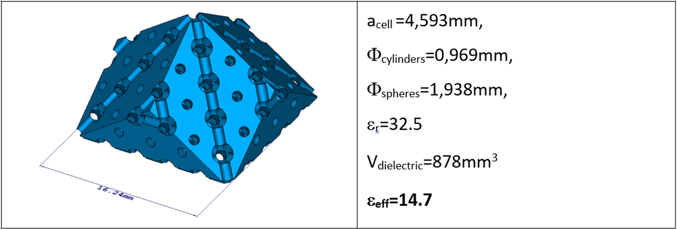
The first step is to determine the filling ratio of the unit cell in order to achieve an effective permittivity of 15. Several sizes of the unit cell a/λ are compatible with the material synthesis, but it is necessary to choose a small enough value to guarantee the homogenization, without creating parts that are too small and incompatible with the 3DCeram stereolithography process [20]. Homogenized effective permittivity is achieved through pairs of values {a/λ; V _obj/V _cell} where a/λ represents the edge of the cubic lattice containing the FCC structures and the ratio V _obj/V _cell defines the volume of the inclusions (i.e. the sections of the cylinders and spheres) relative to the volume of the periodic cell. These values are chosen through the synthesis process, after plotting the possible combinations in Figures 11 and 12. From these results, the ratio V _obj/V _cell chosen is 42%, corresponding to 42% of air inclusions in the material. To minimize the dispersion of the effective index as much as possible, a/λ is set to 0.061, which is high enough to be compatible with the resolution of the stereolithography process. It corresponds to a = 4.59 mm at the chosen frequency.

Figure 11.

Evolution of the effective permittivity with the filling ratio and periodicity. An abacus is used to define the filling ratio.

Figure 11 Long description

Mean effective permittivity The x-axis is labeled, Vobj slash Vcell, with tick labels 0.2, 0.4, 0.6 and 0.8. The y-axis is labeled, a slash lambda, with tick labels 0.05, 0.1, 0.15, 0.2 and 0.25. The z-axis is labeled, Mean effective permittivity, with tick labels 0, 10, 20 and 30. A single surface is shown. The surface is highest near Vobj slash Vcell about 0.2 and a slash lambda about 0.05, at about 30 on the z-axis. The surface decreases as Vobj slash Vcell increases toward 0.8 and as a slash lambda increases toward 0.25, reaching values near 0 to 5 at the far corner. A vertical color scale at the right has tick labels 5, 10, 15, 20 and 25. A dashed line is drawn on the left side of the plot, with a horizontal segment near z about 15 and a vertical segment dropping toward the base near Vobj slash Vcell about 0.4.

Figure 12.

Dispersion of the effective permittivity depending on the filling ratio and periodicity. Abacus used to evaluate the homogenization quality.

Figure 12 Long description

Effective permittivity dispersion. The x-axis is labeled, Vobj slash Vcell, ranging from 0 to 1 with tick labels at 0, 0.2, 0.4, 0.6, 0.8 and 1. The y-axis is labeled, a slash lambda, with tick labels at 0.05, 0.15 and 0.25. The z-axis is labeled, Effective permittivity dispersion, ranging from 0 to 1.5 with tick labels at 0, 0.5, 1 and 1.5. A 3D surface spans the full x and y ranges. The surface is near 0 at low Vobj slash Vcell and rises as Vobj slash Vcell increases, forming a band of repeated peaks along the a slash lambda direction. The highest peaks appear around Vobj slash Vcell near 1 and a slash lambda between about 0.1 and 0.2, reaching close to the top of the z-axis scale near 1.5. A dashed line is drawn on the base plane parallel to the Vobj slash Vcell direction at a slash lambda equals 0.061, with adjacent text, a slash lambda equals 0.061. A vertical color scale at the right runs from 0 at the bottom to 1 at the top, with intermediate tick labels 0.1, 0.2, 0.3, 0.4, 0.5, 0.6, 0.7, 0.8 and 0.9.

In most cases and for most studied lattices, homogeneity is altered for a lattice periodicity (a/λ) greater than 0.1. This is an important consideration in antenna design if the research focuses on the homogeneity of effective permittivity. Note that this parameter must also be chosen in consideration of the practical resolution of the additive manufacturing process, as it can affect the maximum frequency of the design.

The shape of the DRA is based on the concept of using the symmetry planes of the crystalline lattice to create physical objects. One simple way to create an object is to use the shape of the Brillouin zone of the direct crystalline lattice. This zone is defined by the intersection of the lattice’s symmetry planes. Therefore, using the symmetry planes of crystals to shape DRAs allows us to quantify the achievable volumes in relation to the size of the unit cell. In our case, the elementary volume is a rhombic dodecahedron, based on the crystalline lattice theory. It is illustrated in Figure 13. The effective permittivity for these volumes depends on the size of the inclusions (i.e. the sections of the cylinders that comprise the dodecapoles for the FCC lattice) relative to the size of the elementary cells. Once this shape is known, the only remaining step is the evaluation of the diameters of the spheres and cylinders to synthesize the material, as shown in Figure 14.

Figure 13.

Definition of the elementary volume to build the DRA based on the Brillouin lattice of the direct space network. It corresponds to a rhombic dodecahedron for FCC. (a) Physical object based on spheres and cylinders to build the shape with possible scaling (b) and (c).

Figure 14.

Synthesis of the cylinders and sphere diameters of the FCC unit cell.

Figure 14 Long description

Two stacked line graphs share the same horizontal axis label, V obj slash V cell. Top graph: The left vertical axis label is, Effective Index n superscript 2. The right vertical axis label is, n superscript 2 max minus n superscript 2 min. The horizontal axis runs from 0.1 to 0.8. The left vertical axis runs from 0 to 40. The right vertical axis runs from 0 to 0.2. A legend lists three series: MIN n superscript 2 in parentheses theta comma phi in blue, MAX n superscript 2 in parentheses theta comma phi in red and MAX n superscript 2 in parentheses theta comma phi minus MIN n superscript 2 in parentheses theta comma phi in green. The blue and red series decrease from about 28 at V obj slash V cell equals 0.1 to about 4 at V obj slash V cell equals 0.8, with the red series slightly above the blue series throughout. The green series rises from about 0.08 at 0.1 to a peak near 0.2 around 0.25, then decreases to about 0.03 near 0.6, then increases slightly to about 0.05 near 0.75 and ends near 0.04 at 0.8. A vertical dotted guide line is drawn at about V obj slash V cell equals 0.41, with a small callout box near the intersection region. Bottom graph: The vertical axis label is, Diameters in parentheses millimeter. The vertical axis runs from 0.5 to 3.5. Two line series are shown: a red series for sphere diameter and a blue series for cylinder diameter, indicated by nearby text labels. Both series increase with V obj slash V cell. At the vertical dotted guide line near V obj slash V cell equals 0.41, two callouts label the values, Sphere equals 1.938 millimeter and Cylinder equals 0.969 millimeter. The red series is about 0.9 at 0.1 and about 3.1 at 0.8. The blue series is about 0.45 at 0.1 and about 1.55 at 0.8.

The final dimensions of the DRA in the FCC lattice are given in Figure 15. A study of the dispersion of the effective permittivity depending on {θ, φ} directions shows a limited variation contained between 14.63 and 14.7.

Figure 15.

View of the DRA and dimensions to create the physical object.

To validate the structuration process, a CST simulation was performed using a structured DRA in zirconia, compared to a bulk material with ε _eff = 14.7. Both are excited by a microstrip line through a coupling slot on a Rogers RO3003 substrate (ε_r = 3; tan δ = 0.001). The reflection coefficients obtained are in strong agreement, as well as the radiation pattern and gain (Figure 16). Notice that the DRA is based on half part of the structure shown in Figure 13 due to the ground plane.

Figure 16.

Comparison in simulations of the DRA made with FCC and structured lattice in zirconia, and the one made with an equivalent raw material and ε _eff = 14.7. Radiation patterns and reflection coefficient.

Figure 16 Long description

A composite figure with three parts arranged as two 3D plots on the top row and one line graph on the bottom row. A) A 3D farfield surface plot above a rectangular ground plane and a small block shaped structure. A vertical color scale at the right is labeled, db, with tick labels 6.5, 5.51, 4.57, 3.63, 2.44, 1.63, 0.814, 0, minus 4.19, minus 8.37, minus 12.6, minus 16.7, minus 20.9, minus 25.1, minus 29.3, minus 33.5. A small text box lists: Type, Farfield; Approximation, enabled (kR greater than 1); Monitor, farfield (f equals 4.05) [1]; Component, Abs; Output, Realized Gain; Frequency, 4.05; Rad. effic., minus 0.02322 db; Tot. effic., minus 0.02469 db; rzd. Gain, 6.510 db. B) A second 3D farfield surface plot above a rectangular ground plane with a small block shaped structure and a small connector like object near the left side. A vertical color scale at the right is labeled, db, with tick labels 6.58, 5.76, 4.93, 4.11, 3.29, 2.47, 1.64, 0.822, 0, minus 4.18, minus 8.36, minus 12.5, minus 16.7, minus 20.9, minus 25.1, minus 29.2, minus 33.4. A small text box lists: Type, Farfield; Approximation, enabled (kR greater than 1); Monitor, farfield (f equals 4.05) [1]; Component, Abs; Output, Realized Gain; Frequency, 4.05; Rad. effic., minus 0.008005 db; Tot. effic., minus 0.04483 db; rzd. Gain, 6.578 db. C) A line graph with two curves and a grid. The x-axis label is, freq (GHz), with tick labels 3, 3.2, 3.4, 3.6, 3.8, 4, 4.2, 4.4, 4.6, 4.8, 5. The y-axis label is, S11 (dB), with tick labels 0, minus 5, minus 10, minus 15, minus 20, minus 25, minus 30. Two labeled series appear inside the plot: red text, S11 DRA FCC (simulation) and blue text, S11 DRA bulk 14.7 (simulation). Both curves are near 0 decibel at 3 and at 5 and both form a narrow minimum near 4.1. The red curve reaches about minus 20 decibel at its minimum. The blue curve reaches about minus 30 decibel at its minimum.

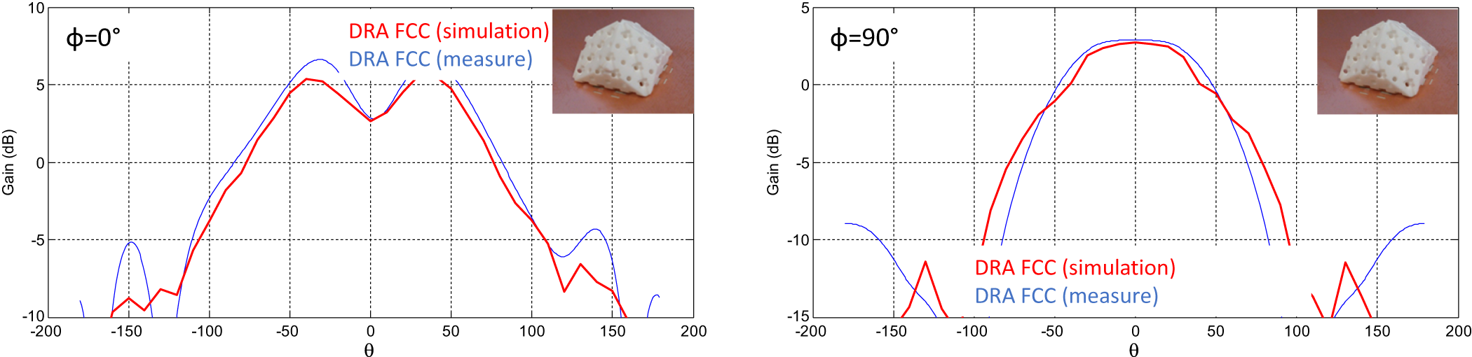
At last, the radiation patterns are measured and compared to the simulation in Figure 17. The agreement is satisfactory. A maximum gain deviation of 2 dB is observed in the ϕ = 0° cut-plane for some directions, with a gain higher in measurement. However, the gain for θ = 0° is very close.

Figure 17.

Radiation pattern comparison for ϕ = 0° and ϕ = 90° in simulation and measurement for the realized DRA based on the FCC lattice.

Figure 17 Long description

Phi equals 0 degrees. The x-axis label is theta, with tick labels from minus 200 to 200. The y-axis label is Gain in decibel, with tick labels at minus 10, minus 5, 0, 5 and 10. Two curves are shown with legend text, DRA FCC (simulation) and DRA FCC (measure). The curves rise from near minus 10 decibel at negative theta values to a broad high region around the center. The simulation curve reaches about 5 decibel near theta around minus 50, dips to about 3 decibel near theta around 0, then rises again to about 5 decibel near theta around plus 50. Both curves fall toward negative values beyond about plus 100 and below about minus 100. A small inset photo at the top right shows a rectangular block with multiple circular holes. Phi equals 90 degrees. The x-axis label is theta, with tick labels from minus 200 to 200. The y-axis label is Gain in decibel, with tick labels at minus 15, minus 10, minus 5, 0 and 5. Two curves are shown with legend text, DRA FCC (simulation) and DRA FCC (measure). Both curves form a rounded peak near theta equals 0 at about 3 to 4 decibel, then decrease toward negative gain values as theta moves toward about minus 100 and plus 100. Additional low segments appear near the far left and far right of the plot area around theta near minus 150 and plus 150, at gains below about minus 10 decibel. A small inset photo at the top right shows a rectangular block with multiple circular holes.

These results validate the proposed approach to creating an “on-demand” material with a specified effective permittivity.

Discussion on the design of mixed index within the same material

One possible extension of this work would be to use 3D printing to create a complex, structured material combining areas with different effective permittivities. This could be used in future projects involving multiband antennas or frequency bandwidth enhancement. To this end, the previous approach was first employed to ascertain whether homogenous building blocks with ε _eff = 10 or ε _eff = 20 could be fabricated using a zirconia raw material.

Two homogeneous bricks, each composed of 5 × 3 unit cells, have thus been fabricated. The first uses an FCC lattice with a periodicity of 11.74 mm. With air cylinders and spheres measuring 2.901 and 5.802 mm in diameter, respectively, this 3D zirconia substrate should exhibit an isotropic effective permittivity of 10 at 1.57 GHz. The entire object measures 58.7 mm × 35.22 mm × 11.74 mm. In this case, the volume ratio of the unit cell air/ceramic is 53.5%/46.5%. To measure the permittivity of the object, the ceramic part is covered with aluminum foil to create a parallelepiped cavity filled with an effective medium of 10. The following procedure is then used to confirm the complex permittivity. First, two windows are cut into the aluminum foil at the two small ends of the object. Two magnetic loops are connected to ports 1 and 2 of a VNA (Vector Network Analyzer) and placed close to the openings. The distance between them and their orientation are optimized to minimize coupling, in order to measure the resonant cavity created by the S21 peaks, which have a level around −40 dB. In this configuration, the first three resonant modes (TE101, TE102, and TE103) can be identified, and their parameters (central frequency and loaded and unloaded Q factor) extracted. We then run a MATLAB code that uses analytic equations for the resonant frequency and unloaded quality factor of a parallelepiped cavity resonator. This code solves these equations numerically, determining the effective complex permittivity of the dielectric medium inside the parallelepiped cavity that matches the measured data for the first three cavity modes. The code considers different sources of inaccuracy, such as dispersion on the outer dimensions of the ceramic brick, error in the VNA’s measurement of the modulus, phase, and frequency, and measurement error in the aluminum foil conductivity, and propagates these in the equations. Using this procedure, the accuracy of the extracted permittivity is close to 0.5%, and the loss tangent is close to 5%.

The conductivity of the aluminum foils was determined using the same procedure as explained in [Reference Feuray, Delage, Abdelghani, Sence, Tantot, Bila, Frigui, Baillargeat, Verdeyme, Delhote and Staelens24] and was found to be 6.15 ± 0.40 MS/m.

The measured complex permittivity for the first use case, which is expected to be 10, is shown in Figure 18, along with the 3D-printed part made out of zirconia.

Figure 18.

(a) 3D-printed zirconia parts for a targeted design ε _eff = 10 and (b) ε _eff = 20. (c) Measured permittivity and loss tangent of the 3D-printed zirconia parts.

Figure 18 Long description

A rectangular block with a repeating raised pattern. A ruler is placed along one edge. The image B showing a rectangular block with a repeating raised pattern. A ruler is placed along one edge. A line graph showing permittivity versus frequency with measured and predicted series. The horizontal axis label is, Frequency, with unit, gigahertz. The horizontal axis range is 1 to 4. The vertical axis label is, Permittivity. The vertical axis range is 1 to 22. The legend lists, Permittivity eps eff equals 10, Predicted value eps eff equals 10, Permittivity eps eff equals 20, Predicted value eps eff equals 20. The plotted values shown next to data points are 9.79, 9.86, 10.16, 19.573 and 20.53. The values 9.79, 9.86 and 10.16 increase across frequency. The values 19.573 and 20.53 increase across frequency. A line graph showing loss tangent versus frequency. The horizontal axis label is, Frequency, with unit, gigahertz. The horizontal axis range is 1 to 4. The vertical axis label is, Loss tangent. The vertical axis range is 0.001 to 0.01. The legend lists, Loss tangent eps eff equals 10, Loss tangent eps eff equals 20. The plotted values shown next to data points are 0.0027, 0.00485, 0.00685, 0.00405 and 0.00270. The values 0.0027, 0.00485 and 0.00685 increase across frequency. The values 0.00405 and 0.00270 decrease across frequency.

The measured effective permittivities at 1.585, 2.118, and 2.753 GHz are 9.79, 9.86, and 10.16, respectively, with an error margin of ±0.5%. When the typical geometrical parameters were checked using a digital microscope, it was found that the average diameter of the air spheres was 140 µm smaller than the theoretical value. The air cylinders are also 110 µm smaller than the designed value. Therefore, the volume of air in a unit cell is slightly smaller than expected, which may explain the lower permittivity of 9.79 at 1.585 GHz, where a value of 10 was expected at 1.57 GHz.

A second version of this 3D part was designed and fabricated. In this case, the objective was an effective permittivity of 20 at 2.1 GHz while still using zirconia and an FCC lattice. Here, a periodicity of 8.3 mm was chosen, with air cylinders and spheres with respective diameters of 1.252 and 2.505 mm. The entire object measures 41.50 mm × 24.90 mm × 8.30 mm. In this case, the unit cell air/ceramic volume ratio is 24/76%. Figure 18(b) shows the fabricated part, and Figure 18(c) shows the measured complex permittivity extracted using the same procedure described previously.

In this case, the TE103 peak was highly asymmetrical, so the measurement of its frequency and Q factor was deemed unsatisfactory. Only the first two modes, at 2.794 and 3.445 GHz, were used. The respective effective permittivities at these two frequencies are 19.573 and 20.53 (±0.5%), compared to the designed value of 20 at 2.1 GHz.

We checked the manufactured dimensions again and found that the air cylinder diameters are 47 µm smaller than predicted. The air spheres also have an average diameter that is 125 µm smaller than expected. This leads to a unit cell in which the percentage of air is slightly smaller than desired.

In terms of loss tangent, one can expect a loss tangent better than 7 × 10⁻⁴ for applications at a few GHz with such 3D zirconia substrates, since the bulk material has a loss tangent of 9.1 × 10⁻⁴ at 5.3 GHz. However, this directly depends on the air/ceramic ratio in the unit cell, as demonstrated in previous sections.

Based on these satisfactory results, an attempt was made to combine the two materials with an FCC lattice structure in order to generate a material with multiple effective permittivity regions. The idea was to create two areas with respective effective permittivities of 10 and 20, separated by a transition area whose effective permittivity would satisfy two conditions. The first condition is that the effective permittivity varies smoothly between the two areas. The second condition is based on mechanical and fabrication constraints. The two opposite sides of the transition area must be connected precisely to the FCC lattice cylinders and spheres in the two regions. It is important to ensure the clean fabrication of the parts after the stereolithography process. Based on these conditions, the effective permittivity of the transition area was set to 14.57. The object was only studied in simulation, with the modal behavior between the homogeneous area block and the structured area with FCC lattices being compared using a full-wave simulation in CST Studio Suite. The dimensions and areas are shown in Figure 19.

Figure 19.

Complex material made of three homogeneous areas (top) and equivalent structured material with FCC lattice based on zirconia to reach the three effective permittivities in the same process (bottom).

Figure 19 Long description

Two parts are shown. The top part labeled ′homog′ depicts a rectangular block divided into three sections, each with different permittivity values. The left section is labeled epsilon equals 10, the middle section is labeled epsilon equals 14.57 and the right section is labeled epsilon equals 20. The dimensions of the block are shown as 72.7 millimeters in height, 72.7 millimeters in width and 72.7 millimeters in depth. The bottom part labeled ′3D′ illustrates a structured material with an FCC lattice. The left section is labeled epsilon equals 10, with sphere diameter equals 5.188 millimeters and cylinder diameter equals 2.994 millimeters. The right section is labeled epsilon equals 20, with sphere diameter equals 3.132 millimeters and cylinder diameter equals 1.666 millimeters. The overall permittivity of the structured material is labeled epsilon equals 32.5. Both parts include a coordinate system in the bottom right corner, indicating orientation.

To validate this approach, an eigenmode study was conducted on the homogeneous areas of the bulk cavity, and the results were compared with those of an eigenmode study on 3D structured material with FCC lattices. The results are shown in Figure 20. The four modes in the homogeneous material with three areas are TE110 (1.533 GHz), TE120 (2.029 GHz), TE130 (2.626 GHz), and TE210 (2.758 GHz).

Figure 20.

View of the H-field inside the homogeneous material with three different areas, compared to the structured FCC material. Comparison for TE110, TE120, TE130, and TE210 modes.

Figure 20 Long description

A comparison of H-field patterns for TE modes in homogeneous material and structured FCC material. Each mode is represented by two heatmaps and a lattice geometry panel. The modes are TE110, TE120, TE130 and TE210, with frequencies of 1.533 gigahertz, 2.029 gigahertz, 2.626 gigahertz and 2.758 gigahertz, respectively. For each mode, the first heatmap shows the field distribution in homogeneous material, while the second heatmap shows the field distribution in FCC material. The heatmaps encode the magnitude of the magnetic field, with a color scale indicating intensity. The lattice panels illustrate the geometric structure of the FCC material. In TE110 mode, the field distribution shows banded structures with concentration near the edges. TE120 mode displays looped patterns with symmetry lines. TE130 mode has central nodes and antinodes, while TE210 mode shows strong field concentration near boundaries. The paired cases generally agree in field patterns, with minor variations in symmetry and intensity across modes. Axes labels and units are not explicitly provided in the image.

Excellent agreement is observed with the FCC structured material because the frequencies of these modes are, respectively, TE110 (1.543 GHz), TE120 (2.032 GHz), TE130 (2.614 GHz), and TE210 (2.752 GHz). Furthermore, the structure of the modes can be seen in Figure 20. The variations are close, even though the FCC lattice slightly disturbs the field lines. It is important to note that the field variation is smooth in the transition area, with all the nulls located in the same position as in the homogeneous material. Based on this validation, this approach could be useful for building complex DRAs like those presented in [Reference Lamotte, Mazingue, Bhatker, Romier, Capet, Delhote, Menudier, Tantot, Thevenot and Elis25, Reference Lamotte, Mazingue, Bhatker, Romier, Capet, Delhote, Menudier, Tantot, Thevenot and Elis26].