1. Introduction
In particle-laden turbulence, the spatial distribution of inertial particles exhibits pronounced non-uniformity, a phenomenon commonly observed in nature and in industrial applications, where clustering or preferential concentration of particles occurs (Monchaux et al. Reference Monchaux, Bourgoin and Cartellier2010, Reference Monchaux, Bourgoin and Cartellier2012). Since the pioneering work of Maxey (Reference Maxey1987), the study of the cluster of inertial particles in flow fields has been well understood through numerical simulations, experiments and theoretical analyses. Early studies (Maxey Reference Maxey1987; Squires & Eaton Reference Squires and Eaton1990; Fessler et al. Reference Fessler, Kulick and Eaton1994) focused on obtaining particle concentration fields and particle behaviour through direct numerical simulation (DNS), then clustering behaviour of particles was also investigated in the experiments (Fessler et al. Reference Fessler, Kulick and Eaton1994; Aliseda et al. Reference Aliseda, Cartellier, Hainaux and Lasheras2002; Wood et al. Reference Wood, Hwang and Eaton2005). As demonstrated in these seminal studies, small inertial particles are found to be predominantly concentrated in regions characterised by high strain and low vorticity (Squires & Eaton Reference Squires and Eaton1990; Wang & Maxey Reference Wang and Maxey1993). Subsequent numerical simulations and experimental studies have further elucidated the mechanism of inertial particle clusters (Chun et al. Reference Chun, Koch, Rani, Ahluwalia and Collins2005; Bec et al. Reference Bec, Biferale, Boffetta, Celani, Cencini, Lanotte, Musacchio and Toschi2006; Goto & Vassilicos Reference Goto and Vassilicos2008; Balachandar & Eaton Reference Balachandar and Eaton2010; Monchaux et al. Reference Monchaux, Bourgoin and Cartellier2012), such as the sweep-sticks mechanism (Chen et al. Reference Chen, Goto and Vassilicos2006; Goto & Vassilicos Reference Goto and Vassilicos2006, Reference Goto and Vassilicos2008), which have been shown to have a significant impact on the behaviour of inertial particles, and the mechanism of inertial particle clusters on dissipative and inertial scales (Bragg et al. Reference Bragg, Ireland and Collins2015). This cluster behaviour has been shown to alter the spatial concentration and collision rate of the particles (Sundaram & Collins Reference Sundaram and Collins1997; Wang et al. Reference Wang, Wexler and Zhou2000), as well as their settling velocity (Wang & Maxey Reference Wang and Maxey1993; Aliseda et al. Reference Aliseda, Cartellier, Hainaux and Lasheras2002).
Several well-established mathematical statistical methods have been used to characterise the preferential concentration of particle distributions (Monchaux et al. Reference Monchaux, Bourgoin and Cartellier2012), such as the box-counting method (Fessler et al. Reference Fessler, Kulick and Eaton1994; Aliseda et al. Reference Aliseda, Cartellier, Hainaux and Lasheras2002), the radial distribution function (RDF) (Wood et al. Reference Wood, Hwang and Eaton2005) and the angular radial distribution function (ADF) (Fong et al. Reference Fong, Amili and Coletti2019). Although these methods have been successfully applied in previous studies, their limitations are, to some extent, unable to give local information about the particles in the cluster region (Monchaux et al. Reference Monchaux, Bourgoin and Cartellier2012; Fong et al. Reference Fong, Amili and Coletti2019; Petersen et al. Reference Petersen, Baker and Coletti2019). The Voronoï division, which can identify the local information of clustered particles and is used by most researchers, has been favoured since Monchaux et al. (Reference Monchaux, Bourgoin and Cartellier2010) introduced this method into particle clustering analysis due to its good stability and visualisation. Based on the advantages of this approach, scholars have provided valuable insights into particle-related phenomena in a wide range of flow configurations from homogeneous isotropic turbulence (Monchaux et al. Reference Monchaux, Bourgoin and Cartellier2010; Tagawa et al. Reference Tagawa, Mercado, Prakash, Calzavarini, Sun and Lohse2012; Dejoan & Monchaux Reference Dejoan and Monchaux2013; Baker et al. Reference Baker, Frankel, Mani and Coletti2017) to wall turbulence (Sumbekova et al. Reference Sumbekova, Cartellier, Aliseda and Bourgoin2017; Petersen et al. Reference Petersen, Baker and Coletti2019; Zhu et al. Reference Zhu, Pan, Wang, Liang, Ji and Wang2021; Cui et al. Reference Cui, Ruhman and Jacobi2022; Wang et al. Reference Wang, Chen and Zheng2024). In these studies, preferential clustering of particles is considered to be the response of particles to turbulence, i.e. particles are clusters in a highly inhomogeneous manner in a specific region of the flow. For example, in both simulations (Monchaux et al. Reference Monchaux, Bourgoin and Cartellier2010; Baker et al. Reference Baker, Frankel, Mani and Coletti2017) and experiments (Petersen et al. Reference Petersen, Baker and Coletti2019; Zhu et al. Reference Zhu, Pan, Wang, Liang, Ji and Wang2021; Cui et al. Reference Cui, Ruhman and Jacobi2022), heavy particles have been found to avoid regions of high vorticity and stay within regions dominated by high strain. In wall-bounded flows, clustered particles are evident in the form of particles drifting towards the wall and accumulating as low-velocity streaks (Soldati & Marchioli Reference Soldati and Marchioli2009; Berk & Coletti Reference Berk and Coletti2023), flow sweeping and ejection events in these flows play a crucial role in influencing particle clustering. In addition to this, the clustering of particles also changes the dynamics and kinematics of particles, i.e. the settling velocity of particles in the clustered region is faster than their particle velocity (Fong et al. Reference Fong, Amili and Coletti2019) and the clustering of particles leads to a significant increase in the rate of local inter-particle collisions (Ernst et al. Reference Ernst, Sommerfeld and Laín2019). In our previous study, we have revealed that the particle–wall interactions significantly affect the preferential concentration of particles near the wall (Wang et al. Reference Wang, Chen and Zheng2024). In the present study, the authors investigated the phenomenon of particle clusters in particle-laden flow, delineating them based on Voronoï delimitation in the presence of wall processes such as particle impact to the wall and rebounding.
It is important to note that the morphological and kinematic analysis of clusters can be performed based on the identification of particle clusters using the Voronoï diagram method, filtered by additional self-similarity conditions and thus obtaining clusters. As stated in the definition of particle clusters by Monchaux et al. (Reference Monchaux, Bourgoin and Cartellier2012): ‘groups of particles that remain close to one another on time scales long compared with some turbulence time scale’. This suggests that particle clusters can be identified by the distribution of the physical spatial concentration of particles in the short-term (Monchaux et al.. Reference Monchaux, Bourgoin and Cartellier2012; Baker et al. Reference Baker, Frankel, Mani and Coletti2017; Liu et al. Reference Liu, Shen, Zamansky and Coletti2020). While analysing the properties associated with particle clusters in homogeneous isotropic turbulence, Baker et al. (Reference Baker, Frankel, Mani and Coletti2017), using the Voronoï diagram method, gave a clear topological definition of particle clusters in multiphase flows. They pointed out that to avoid spurious edge effects, while defining as clusters the set of particles in which the cells with the area (volume) below a threshold belong to the same connectivity group, it should be appended that the area (volume) of the neighbouring Voronoï cells of the clustered particles should also be less than the threshold at which clustering occurs. Therefore, a clear distinction between clustered particles and a clustered cluster is essential for the accurate identification and analysis of particle clusters. However, the current studies of particle clusters have mainly focused on isotropic homogeneous flow (Baker et al. Reference Baker, Frankel, Mani and Coletti2017; Liu et al. Reference Liu, Shen, Zamansky and Coletti2020) and vertical channels (Fong et al. Reference Fong, Amili and Coletti2019). The distribution behaviour and related properties of particle clusters in the case of particle–wall interaction have received rare attention from researchers, thereby impeding our comprehension of the behaviour of clusters in wall turbulence. Therefore, in this study, we further investigate the effect of different wall actions on the particle clusters formed by inertial particles in wall turbulence based on our previous work (Wang et al. Reference Wang, Chen and Zheng2024). Unlike the previous study (Wang et al. Reference Wang, Chen and Zheng2024), in this paper, we focus on the study of clusters with three or more interconnected clustering particles.
Particle motion in the near-wall region is an extremely complex process, mainly due to the anisotropy of the velocity field at the wall caused by the presence of rigid boundaries, which in turn complicates the flow field, a change that significantly affects the dynamics of small particles in particular (Brandt & Coretti Reference Brandt and Coletti2022). In addition, particle motions near the wall show diverse patterns, and in addition to settling processes, particle–wall interactions and their coupling effects further increase the complexity of particle motions (Marchioli & Soldati Reference Marchioli and Soldati2002; Fong et al. Reference Fong, Amili and Coletti2019; Wang et al. Reference Wang, Chen and Zheng2024). Particle motion in the near-wall region exhibits highly complex dynamics, which mainly stems from the flow field anisotropy induced by the rigid wall surface and its significant effect on small-scale particle dynamics (Brandt & Coretti Reference Brandt and Coletti2022). Existing studies have revealed the physical mechanism of this process from different perspectives: Tanière et al. (Reference Tanière, Oesterlé and Monnier1997) observed, for the first time, the phenomenon of dramatic fluctuations in the velocity of near-wall particles through wind tunnel experiments and attributed it to the bouncing motion of the particles; Righetti & Romano (Reference Righetti and Romano2004) studied glass beads in water with a volume fraction of 10
 $^{-3}$
and found that the particle–wall entrainment-deposition process triggered significant turbulence modulation effects, while boundary layer measurements by Gerashchenko et al. (2012) showed that particle acceleration fluctuations were enhanced with increasing inertia, a phenomenon that is quite different from the pattern found in anisotropic turbulence (Bec et al. Reference Bec, Biferale, Boffetta, Celani, Cencini, Lanotte, Musacchio and Toschi2006). The quantitative measurements of Baker & Coletti (Reference Baker and Coletti2021) further revealed that the particle acceleration fluctuations were not as strong as those found in isotropic turbulence. Quantitative measurements further revealed that particles in contact with the wall always maintain a higher velocity of motion than the local fluid in the near-wall region. Recently, Zheng et al. (Reference Zheng, Wang and Zhu2021) systematically investigated the regulation mechanism of particle–wall (P-W) interactions on a turbulent superscale structure (SVLSM) by designing different particle release schemes.
Numerous studies have shown that particles tend to cluster in regions of the flow with specific topological features and their spatial distribution is closely related to the local flow field structure. For example, both numerical simulations and experimental observations show that heavy particles actively avoid the vorticity-dominated high-rotation region and tend to cluster in the strain-rate-dominated shear region (Aliseda et al. Reference Aliseda, Cartellier, Hainaux and Lasheras2002; Marchioli & Soldati Reference Marchioli and Soldati2002; Bernardini Reference Bernardini2014; Petersen et al. Reference Petersen, Baker and Coletti2019; Zhu et al. Reference Zhu, Pan, Wang, Liang, Ji and Wang2021). Marchioli & Soldati (Reference Marchioli and Soldati2002) showed that particles in the vicinity of the wall exhibit preferential clustering during sweeping and ejection events, the so-called ‘turbophoresis’ phenomenon; these events are usually associated with hairpin vortices. This implies that the formation of particle clusters is also directly related to these coherent structures (Sardina et al. Reference Sardina, Schlatter, Brandt and Picano2012; Berk & Coletti 2020; Zhu et al. Reference Zhu, Pan, Wang, Liang, Ji and Wang2021). Is it possible that the distribution and formation of particle clusters in wall flow are also influenced by fluid behaviour? There is still a lack of systematic studies on the mechanisms by which particle–wall interactions affect particle clustering in wall flow. Therefore, an in-depth study of clusters in wall flow is needed.
In this paper, we use the Voronoï division technique to identify clusters based on the definitions of particle clusters by Baker et al. (Reference Baker, Frankel, Mani and Coletti2017) and Zhu et al. (Reference Zhu, Pan, Wang, Liang, Ji and Wang2021) for net settling and wall-released particle distributions, respectively, in a wind tunnel environment. Using this definition, we identify the local information of the clusters and characterise their concentration, velocity and morphological structure under different operating conditions. The paper is structured as follows: a brief description of the experimental set-up and the methodology for identifying particle clusters is presented in § 2; § 3 presents results in terms of cluster topology and conditional flow statistics in addition to spatial distributions of cluster concentrations and velocities; and § 4 contains conclusions and discussion.
Experimental set-up and location of racks for measuring instruments. (a) Wind tunnel measurement set-up; (b) particle release modes under two operating conditions; (c) enlarged view of the FOV of the CCD camera.

2. Method
2.1. Experimental setting
All measurements were carried out along the
 $x{-}z$
plane shown in figure 1 using the same set-up procedure as Wang et al. (Reference Wang, Chen and Zheng2024), which is only briefly described here. The experiments were conducted in the Multifunctional Environmental Wind Tunnel at Lanzhou University. Two distinct particle-release configurations were employed: Case 1 (top-released), where particles were introduced from the top; and Case 2 (bottom-lifted), where particles were locally lifted from the wall surface. Compared with Case 2, the top-released particles in Case 1 acquired greater settling momentum and kinetic energy due to gravitational potential energy conversion. Consequently, particle–wall interactions were significantly more intense in Case 1 than in Case 2, where particles originated near the wall. By maintaining identical wind speeds and sand particle properties, this experimental set-up enabled controlled variation in particle–wall interaction strength, as shown in figure 1. In Case 1, sand particles were introduced through a feeder at the wind tunnel entrance, descending from the top before being transported downstream by wind shear. In Case 2, particles entrained by wall shear stress underwent continuous wall collisions and rebounds, developing into a fully established saltation flow regime. For the measure of particle–wall interaction particles, we use the number of upward particles/total number of particles given by Zheng et al. (Reference Zheng, Wang and Zhu2021) to portray the particle–wall strength
 $\zeta =n_{up}/n_{up}+n_{down}.$
Statistically, we found that near the wall (
 $z^{+}\lt 300$
), interaction is the same for both working conditions (
 $\zeta \approx 0.5$
). Compared with Case 1, the decreasing rate of
 $\eta$
with height is much lower in Case 2, implying that Case 2 maintains more active near-wall activity (Liu et al. Reference Liu, Feng and Zheng2022).
The cross-sectional dimension of the wind tunnel was
 $1.3\,\rm m \times 1.4\,\rm m$
and the length of the experimental section was 20 m. In this study, along-flow and vertical imaging is adopted, and the laser is a double-pulse, 500 mj pulse−1, emitting green light at a wavelength of 532 nm with an operating frequency of 4 Hz. The measurement position is 10 m downstream of the wind tunnel test section, and the origin of the metrology coordinates is set at the lower left corner of the acquisition field of view (FOV), which can provide
 $8.02\delta \times 1.34\delta$
field of view information, and this method can not only resolve the small-scale fluctuations and large-scale motions, but also ensure the convergence of the large-scale structure. For two-dimensional (2-D) particle image velocimetry (PIV) measurements, di-2-ethylhexyl sebacate (DEHS) droplets with a diameter of 0.3–3
 $\unicode{x03BC}$
m were used as tracer particles in the flow phase in this experiment. Four cameras (FlowSense EO 16MP) with a resolution of
 $4920\times 3280 \,\rm pixel$
were connected via a synchroniser and arranged along the flow direction, where the sampling frequency is 4 Hz and the magnification is 80
 $\unicode{x03BC}$
m
 $\,\rm pixel^{-1}$
. The cross-section of
 $32 \times 32\,\rm pixel$
size is selected as the query region for image processing, which has 75
 $\%$
correlation in the flow direction and vertical direction, and the velocity field node spacing is
 $\Delta x\times \Delta z =0.7 \times 0.7\,\rm mm$
. The TBL curves of this paper are shown in the figure 1. The average particle size of the particles is approximately
 ${d}_p=203$
 $\unicode{x03BC}$
m, and the root-mean-square (r.m.s.) of the particle size is 210.2
 $\unicode{x03BC}$
m. The laser and camera (charge-coupled device, CCD) settings are shown in figure 1. Using this approach not only resolves small-scale fluctuations but also the large-scale motions. In the experiments, we can simultaneously capture the dynamics of flow and particles (Zheng et al. Reference Zheng, Wang and Zhu2021). The approximate steps of the algorithm are as follows: (i) the recorded image is divided into a particle field, which is used to calculate the particle position and velocity, and a tracer particle field, which is used to calculate the flow field, based on the pixel size and brightness; (ii) quantifying the velocity field of the fluid in the tracer image using PIV; and (iii) quantifying the position and velocity of particles in particle images using particle tracking velocimetry (PTV). We used adaptive PIV in DynamicStudio software and selected a 32 pixel
 $\times$
32 pixel pixel area as the query window, with a correlation of 75
 $\%$
in the flow and droop directions (Liu et al. Reference Liu, Feng and Zheng2022; Wang et al. Reference Wang, Chen and Zheng2024). Statistics for each experimental case were calculated from 3200 pairs of images.
The main parameters of the continuous phases are presented in table 1. The properties of the fluids approximate those of air at standard temperature and pressure. In all the experiments, the statistical data were collected under the same clear flow conditions: the free flow rate was fixed at
 $U_\infty =9 \,\rm m\,s^{-1}$
which was to achieve better control under sandy flow conditions. This method is more controllable compared with the variation of flow conditions in the case of sand-containing flow, thus achieving a control variable that facilitates a more accurate comparison of the geometrical morphology and distributional characteristics of the clusters under the two different modes of releasing particles.
Fluid phase physical parameters.

The friction Reynolds number
 ${Re}_\tau =u_\tau \delta /\nu =3950$
is obtained by fitting the wind speed profile to the boundary layer thickness
 $\delta$
and the friction wind speed
 $u_\tau$
. The boundary layer shape factor H = 1.27. Specific information on the particles is shown in table 2. The sand particles used in this experiment are screened desert natural sand particles and the ratio of particle to fluid density is
 $\rho _p/\rho _{\!f}=2148$
. The average particle size of the particles is approximately
 $\langle {d}_p\rangle =203\,\rm \unicode{x03BC}m$
, and the r.m.s. of the particle size is 210.2
 $\,\rm \unicode{x03BC}m$
. The relaxation time of the particles can be expressed as
 $\tau _{\!p}=\rho _p{d}_p^{2}/18\nu \rho _{\!f} (1+0.15{Re}_p^{0.687})$
(Kumaran Reference Kumaran2003). Particle Reynolds number
 ${Re}_p={d}_p|\boldsymbol{u_{\!p}}-\boldsymbol{u_{\!f}}|/\nu$
, which based on the particles’ diameter and slip velocity relative to the fluid. Note that the maximum slip velocity is
 $\boldsymbol{u_r}=|\boldsymbol{u_{\!p}}-\boldsymbol{u_{\!f}}|$
(Kiger & Pan Reference Kiger and Pan2002), which was obtained from PIV and PTV measurements. The Stokes number of a particle is defined as the ratio of the characteristic time of the fluid, i.e.
 $St_{\!p}=\tau _{\!p}/\tau _{\!f}$
, and
 $\tau _{\!f}$
can be taken in two general ways, either on the Kolmogorov time scale
 $\tau _\eta \approx (\nu \delta /(0.1U_\infty )^{3})^{1/2}$
or on the time scale of the largest turbulent eddy
 $\tau _L\approx \delta /(0.1U_\infty )$
(Tanière et al. Reference Tanière, Oesterlé and Monnier1997). Here,
 $St_L$
and
 $St_l$
can be obtained by replacing
 $\tau _{\!f}$
with
 $\tau _L$
and
 $\tau _\eta$
, respectively; table 2 estimates the particle Stokes numbers
 $St_l=77.143$
and
 $St_L=0.780$
using
 $\tau _\eta$
and
 $\tau _L$
, respectively. This implies that the particle motion in this experiment is neither in a pure suspension state
 $(St_l)\lt \!\lt 1$
nor in a pure saltation state
 $St_L\gt\! \gt 1$
, but is simultaneously affected by both phases of motion together. In addition to this, the volume fraction of the particles under Case 1 and Case 2 conditions are
 $1.1\times 10^{-4},1.4\times 10^{-4}$
, respectively.
Properties of tested sand grains.

2.2. Voronoï diagramming to identify clusters
To analyse particle clusters formed by near-wall particles, first, we use the Voronoï delineation technique to identify particles where clustering occurs. Since its pioneering application to particle-laden flows by Monchaux et al. (Reference Monchaux, Bourgoin and Cartellier2010), the Voronoï method has gained widespread adoption in multiphase flow research owing to its algorithmic stability and objective quantification capabilities. The technique’s robustness has been demonstrated through extensive experimental validations (Sumbekova et al. Reference Sumbekova, Cartellier, Aliseda and Bourgoin2017; Fong et al. Reference Fong, Amili and Coletti2019; Petersen et al. Reference Petersen, Baker and Coletti2019; Cui et al. Reference Cui, Ruhman and Jacobi2022) and numerical investigations (Monchaux et al. Reference Monchaux, Bourgoin and Cartellier2012; Baker et al. Reference Baker, Frankel, Mani and Coletti2017), establishing it as a reliable approach for cluster characterisation in both laboratory and computational settings. Here is a brief review. The Voronoï diagram method divides each particle in the FOV into associated cells based on the spatial location of the particle (a cell-like topology), where each cell contains a closer set of particle points than the other cells. The inverse of the area A of each elementary cell is equal to the concentration of the localised particles,
 $c=1/A$
, so the study of the Voronoï area field is strictly equivalent to the study of the concentration field of the localised particles. In addition, the Voronoï area is naturally evaluated for each particle present in the field, and since there is no a priori choice of length scale, the obtained local concentration field pattern is obtained at an intrinsic spatial resolution (Monchaux et al. Reference Monchaux, Bourgoin and Cartellier2012). A Voronoï cell analysis of the two sets of experimental data revealed that the clustering determination threshold
 $\gamma$
was insensitive to changes in the normal height of the wall. The
 $\gamma$
values obtained in this experiment fall within the discrete range reported in previous studies (Monchaux et al. Reference Monchaux, Bourgoin and Cartellier2012; Wang et al. Reference Wang, Chen and Zheng2024). It is worth noting that the choice of the height of the statistical region significantly affects the results of the determination of the clustering threshold, which is an issue that requires special attention when applying the Voronoï analysis method. For this reason, in this study, the same statistical region corresponding to the height is used for clustering cell analysis in both working conditions, and this strategy effectively reduces the systematic error caused by the difference in statistical regions.
In addition, for each particle in the statistical FOV, in contrast to the box counting method and radial function, Voronoï division not only has no a priori length scale choice, but also makes it possible to make the corresponding spatial Voronoï tuple based on the physical spatial location of each particle delineation (Monchaux et al. Reference Monchaux, Bourgoin and Cartellier2012). The main reference for distinguishing clustering from sparsity is the statistical characteristics of random Poisson distributed particles (Squires & Eaton Reference Squires and Eaton1990; Aliseda et al. Reference Aliseda, Cartellier, Hainaux and Lasheras2002; Monchaux et al. Reference Monchaux, Bourgoin and Cartellier2010). The probability distribution function (p.d.f.) of the Voronoï divisions of the tuples of particles with clustering, which are normalised by their mean
 $\bar{A}$
(here and later, the pointed brackets denote the coefficient of integration average) area
 $\gamma =A/\bar{A}$
, is much wider than that of the random Poisson distribution, which follows a
 $\varGamma$
distribution for the area of the random Poisson distribution Voronoï tuples:
 ${\rm p.d.f.}(\gamma )=343/15\sqrt {7/2\pi }\gamma ^{5/2}{\rm exp}(-7/2\gamma )$
(Ferenc & Néda Reference Ferenc and Néda2007). It has been observed that the p.d.f. of the particle elementary cell area in a particle field where clustering occurs is much wider than the distribution in the case of a random Poisson distribution (Monchaux et al. Reference Monchaux, Bourgoin and Cartellier2010). By comparing the p.d.f. of the experimentally obtained Voronoï cell area with the
 $\varGamma$
distribution, the first intersection point obtained is set to be the dimensionless threshold of the clustering area
 $\gamma$
. This yields the clustering threshold of the Voronoï cell area,
 $A^{*}=\gamma \bar{A}$
, below where
 $A^{*}$
cell (i.e.
 $A\lt A^{*}$
) particles are considered clustering particles (Monchaux et al. Reference Monchaux, Bourgoin and Cartellier2010). In contrast,
 $\gamma$
is largely independent of particle sampling and, in addition to this, has quite excellent robustness (Monchaux et al. Reference Monchaux, Bourgoin and Cartellier2012). In wall turbulence, the particles are unevenly distributed along the wall normally, and it has been investigated to normalise the area obtained from the division using the mean values of the different flow layers, and to determine the clustering and evacuation thresholds by means of probability density functions. In this paper, we refer to the method of elementary statistics of particle composition in shear flow of Sumbekova et al. (Reference Sumbekova, Cartellier, Aliseda and Bourgoin2017) and Zhu et al. (Reference Zhu, Pan, Wang, Liang, Ji and Wang2021) for the treatment of data from this experiment. That is, they are normalised using the local mean area. Figure 2(a–c) shows the results of analysing the spatial distribution of particles by the Voronoï division method within the local observation FOV (for display purposes, we chose the FOV
 $2.0\delta \times 1.2\delta$
). As illustrated in figure 2(a), the Voronoï division is based on the particle positions, whereby cells that fall below the clustering threshold are identified as particles within the cluster region. Figure 2(b) presents a filtered view of the cluster region, based on the condition outlined previously. The blue cells in this figure indicate not only particles connected to form clusters but also isolated single particles.
(a) Demonstration of the 2-D Voronoï division of local
 $2\delta \times \delta$
for Case 1; (b) blue-stained cells are granular cells judged to be clustered using Voronoï delineation; (c) clusters of particles identified based on clustering, with orange-stained interconnected clustered particles; (d) comparison of the experimentally derived Voronoï cell map probability density function (p.d.f.) with the random Poisson distribution and
 $\varGamma$
distribution function, where the red line is the experimental value and the black is the random distribution (RPP). Where
 $\gamma =A_{\textit{cell}}/\langle A_{\textit{cell}}\rangle$
, the clustering threshold
 $\gamma _{A}$
can be determined based on the deviation of the two; (e) all p.d.f.s for
 $\log (A_{\textit{cell}})$
of Voronoï cells at different heights at values
 $\chi =(\log (A_{\textit{cell}})-\langle \log (A_{\textit{cell}})\rangle )/\sigma _{\textit{log} (A_{\textit{cell}})}$
centred on the mean and normalised by the standard deviation.

In this study, we employ the Voronoï analysis method to identify particle clusters, adopting the operational definitions established by Baker et al. (Reference Baker, Frankel, Mani and Coletti2017) for homogeneous isotropic turbulence and Zhu et al. (Reference Zhu, Pan, Wang, Liang, Ji and Wang2021) for net settling distributions in a wind tunnel. Baker et al. (Reference Baker, Frankel, Mani and Coletti2017) attribute cluster formation to turbulent velocity field effects, defining particle clusters as interconnected groups of clustering particles. They introduced a volume-scale threshold, considering clusters statistically significant when their volume exceeds
 $8\eta ^{3}$
(where
 $\eta$
represents the flow’s characteristic scale). Zhu et al. (Reference Zhu, Pan, Wang, Liang, Ji and Wang2021), building upon Petersen et al.’s (Reference Petersen, Baker and Coletti2019) statistical approach, defined clusters based on connectivity criteria – specifically requiring particle structures to be connected to at least three neighbouring clustering cells. In addition, three or more interconnected clustering particles (or Voronoï cells) were defined as clusters concerning the treatments of Petersen et al. (Reference Petersen, Baker and Coletti2019) and Zhu et al. (Reference Zhu, Pan, Wang, Liang, Ji and Wang2021). This resulted in clusters composed of neighbouring Voronoï units, as shown in figure 2(c). The orange Voronoï units indicate the structure of the particle clusters. It can be observed that the particle clusters away from the wall show a stripe pattern. The statistical analyses show that particle–wall interactions significantly reduce the size of clustering of particle clusters in the near-wall region in the wall turbulence. The number of particles within particle clusters formed under wall turbulence conditions is significantly reduced compared with homogeneous isotropic turbulence. Quantitative analyses showed that the largest particle clusters had a particle number order of only O(10). Figure 2(d) illustrates the process of determining the clustering threshold by dividing the p.d.f. of the cell area by the Voronoï units, which determines the clustering threshold
 $\gamma _{A}$
by the
 $\varGamma$
distribution, and translates into the threshold area
 $A^{*}$
. However, the condition of clustering (
 $A\lt A^{*}$
) is a necessary but not sufficient condition for particles to belong to a cluster (Baker et al. Reference Baker, Frankel, Mani and Coletti2017), so further differentiation is needed. Figure 2(e) then demonstrates the properties of the Voronoï cells at different heights in Case 1 that conform to a quasi-log-normal distribution after log-normalisation, where
 $\chi =(\log (A_{\textit{cell}}-\langle \log (A_{\textit{cell}}\rangle )/\sigma _{\textit{log} (A_{\textit{cell}})}$
, a behaviour that has been used to characterise the distribution of particles through the standard deviation of the cells of the element (Monchaux et al. Reference Monchaux, Bourgoin and Cartellier2010). The next and final step of identifying clusters is to consider whether the Voronoï cells composed of particles (
 $A\lt A^{*}$
) in these clustered regions are connected into sets defined as clusters. The understanding of preferential concentration in previous studies has shown that turbulence-driven particle clusters have topological features that reflect the dynamics of the underlying flow (Baker et al. Reference Baker, Frankel, Mani and Coletti2017; Zhu et al. Reference Zhu, Pan, Wang, Liang, Ji and Wang2021). In particular, flow structures have been shown to have varying degrees of self-similarity and to exhibit corresponding fractal features (Moisy & Jiménezl Reference Moisy and Jiménez2004; De Silva et al. Reference De Silva, Philip, Chauhan, Meneveau and Marusic2013), while at the same time, inertial particles in turbulent flows have been shown to follow self-similar distributions (Goto & Vassilicos Reference Goto and Vassilicos2006, Reference Goto and Vassilicos2008; Petersen et al. Reference Petersen, Baker and Coletti2019; Zhu et al. Reference Zhu, Pan, Wang, Liang, Ji and Wang2021; Cui et al. Reference Cui, Ruhman and Jacobi2022; Wang et al. Reference Wang, Chen and Zheng2024). In the process of identifying particle clusters, an additional condition is usually imposed: the clusters must be large enough to exhibit self-similarity. This condition is relatively reasonable for particles moving only under the influence of a flow field. This is because if clusters are identified only by interconnected clustered particle units, particles that happen to be nearby may be incorrectly identified as part of the cluster. In transient snapshots, this randomness is indistinguishable unless the historical trajectory of the particles can be traced. The movement of inertial particles near the wall surface increases the frequency of such random events. Therefore, the effect of particle motion near the wall can be somewhat eliminated by the ‘condition that the clusters are sufficiently large and self-similar (this self-similarity can be filtered by whether the corresponding fractal structure is satisfied)’ proposed by Baker et al. (Reference Baker, Frankel, Mani and Coletti2017). Thus, by imposing the condition that clusters must be sufficiently large and self-similar, the effect of particles moving near the wall can be eliminated to some extent, but this also leads to a lack of research on the nature of particle clusters under particle–wall interaction. This limitation may overlook the importance of cluster properties in particle–wall interactions. Considering the above-mentioned factors, in this paper, based on clustered particles, three or more interconnected clusters of clustered particles are defined as a cluster, and clusters composed of different numbers of particles are classified and discussed.
Scatter plot of local particle concentration in the
 $x{-}z$
plane via the overall dimensionless particle concentration
 $C_{a}$
:
 $C_{0}/C_{a}$
and clusters concentration
 $C_{C}/C_{a}$
in the
 $x{-}z$
plane after dimensionless quantisation of the overall particle concentration
 $C_{a}$
.

3. Results and discussion
In this section, we specify the notation of the relevant variables to facilitate the following discussion and analysis. In this paper, a specification of the notation of the relevant variables is given. The subscript
 $C$
(capital letter) denotes the physical quantity associated with the cluster. It is specified that
 $A_{C},C_{C},N_{C}$
denote the area of the Voronoï diagram cell of the cluster (the sum of the areas of the individual particles in the cluster), the concentration in the cluster and the number of particles in the cluster, respectively. Here,
 $U_{c}, W_{c}$
and
 $u_{c}, w_{c}$
denote the flow direction, the vertical mean velocity and the pulsation velocity of the cluster, where the mean value of the velocities of all the particles in the cluster is specified to be the mean velocity of the cluster, and the mean value of the pulsation velocity of each of its individual particles is specified to be the value of the pulsation of the cluster. It should be noted that the concentration about the cluster here is based on the ratio of the number of particles in the cluster and the cluster area
 $A_{C}$
, i.e.
 $C_{C}=N_{C}/A_{C}$
(Baker et al. Reference Baker, Frankel, Mani and Coletti2017). Parameters with subscript
 $c$
are all the particles that satisfy the clustered condition by Vorinoi analysis including particle clusters with three or more interconnected particles, and the other identified clustering particles, e.g.
 $u_{c},w_{c}$
, are the instantaneous streamwise and vertical velocities of the clustered particles, respectively; The subscript
 $a$
denotes the physical quantity corresponding to all particles in the statistical field of view,
 $A_{a},C_{a},N_{a}$
mentioned later denotes the area of all Voronoï cells in the statistical field of view, the concentration of all particles and the total number of particles in the field of view, respectively. Here,
 $U_{a},W_{a}$
and
 $u_{a},w_{a}$
denote the overall particle flow direction, the velocity in the vertical direction and the corresponding pulsation velocity. Other symbols appearing in the text are described at the corresponding locations.
3.1. Concentration of clusters
Figure 3 shows the distribution of clusters concentration with height through the overall particle concentration Ca
dimensionless in their respective statistical fields of view for both cases. For presentation purposes, a FOV of approximately
 $4\delta \times 0.5\delta$
has been chosen to show the distribution of particle concentrations. The concentration distribution is given by box counting, where the length of each box is the entire statistical field of
 $4\delta$
and the width is approximately 3.2 mm (approximately
 $0.017\delta$
). The concentration
 $C_{0}$
(i.e. the local concentration) of particles within each interval was statistically calculated at intervals of 3.2 mm (approximately
 $0.017\delta$
) along the plumb line, and the mean value of the cluster concentration
 $C_{C}$
over the same area was given as the cluster concentration. After making dimensionless the mean
 $C_{a}$
of the overall particle concentration within the statistical field of view of both, the scatter plot of the distribution of clusters concentration in the vertical direction shown in figure 3 can be obtained. Through the statistics, the average concentration
 $C_{a}$
of the whole statistical field of view and all the particles in Case 1 and Case 2 are 0.04 and 0.11, respectively, and it is obvious that the average concentration of particles in Case 2 is much larger than that in Case 1. As illustrated in figure 3, the initial presentation of data is in the form of a scatter plot, which demonstrates the relationship between the local particle concentration (
 $C_{0}/C_{a}$
) and height. The blue boxes and purple upper triangles represent the distribution of particle concentrations within a vertical spacing of
 $0.017\delta$
for the specified conditions of Case 1 and Case 2. In Case 1 conditions, the concentration of particles decreases with increasing height, while in the corresponding Case 2, the local concentration of particles remains almost constant when
 $z/\delta \lt 0.12$
, but in contrast, its concentration decreases with increasing height when
 $z/\delta \gt 0.12$
. This also reflects, to some extent, the difference in the spatial distribution of the two different initiating particles. This trend of decreasing particle concentration with height at the near-wall surface is consistent with that observed in previous studies (Fong et al. Reference Fong, Amili and Coletti2019; Zhu et al. Reference Zhu, Pan, Wang, Liang, Ji and Wang2021; Wang et al. Reference Wang, Chen and Zheng2024), i.e. all show concentration peaks in the near-wall region.
However, a notable distinction emerges between Case 1 and Case 2: for particles initiated via laying down on the wall, a more extensive region of high concentration exists in the near-wall region. Conversely, the near-wall concentration peak for the net settling condition in Case 1 rapidly decays, resulting in the absence of a continuous region of high concentration. This feature distinguishes the behaviour of particles under near-wall conditions from the distribution of particles in anisotropic uniform flow. Furthermore, a plot of the variation of clusters concentration along the vertical height is provided in figure 3. It is important to note that the calculation of clusters concentration differs from the calculation of particle concentration in a local area, as previously described. The former is a purely box-counting method to obtain the local particle concentration, and the calculation of the overall particle concentration,
 $C_{a}$
, is also included. Conversely, the calculation of clusters’ concentration is based on the identification of clusters. The ratio of the number of particles in clusters to the area of the clusters itself is defined as the concentration of a single cluster (the cluster area is the sum of the areas of the Voronoï cells divided by the cluster particles after Voronoï division). The concentration of clusters in a given height area can be obtained by averaging the cluster concentrations at that height, with a vertical spacing of
 $\Delta z=0.017\delta$
. As illustrated in figure 3, the red circles and green inverted triangles represent scatter plots of the distribution of clusters concentrations along the vertical direction in Cases 1 and 2, respectively. In comparison with the local particle concentration, the clusters concentration is always higher than the value of the local particle concentration at the same height, and the maximum value reaches more than three times the local concentration (the maximum cluster concentration reaches 3.8 times the local particle concentration in Case 1 and 3.1 times in Case 2). Not only that, but the clusters concentration also tends to decrease with height. Given the cluster identification method, the clusters in Case 1 are truncated around
 $z/\delta =0.4$
, while those in Case 2 appear to be below the overall average concentration. The higher clusters particle concentration than the local particle concentration does not provide a complete picture of the spatial distribution of clusters concentrations. Although the clusters concentration shows the spatial distribution of clusters to some extent, this statistic is coupled to the number of cluster particles, and it is not possible to visualise the spatial changes in the size of the clusters themselves.
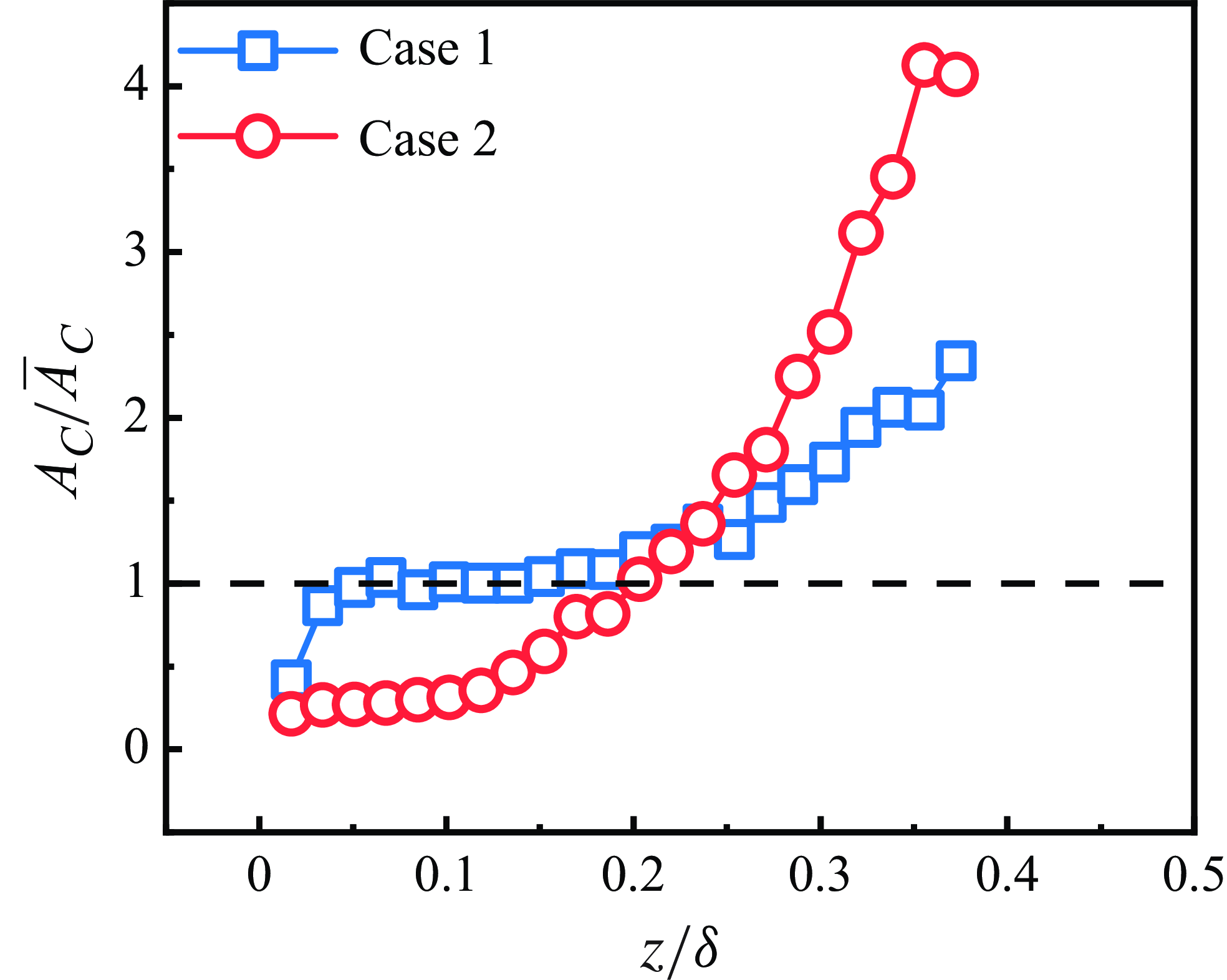
Figure 4 shows a schematic representation of the variation in the dimensionless posterior of the mean cluster area with height. This figure facilitates the visualisation of the trend in the size of the cluster area with height for the two cases. It is evident that the Voronoï metapodial area of the clusters in both Case 1 and Case 2 increases with plumb, with the latter growing at a faster rate than the former after
 $z/\delta =0.12$
. The difference between the two cases is also obvious, as in Case 1, near the near wall, the cluster size is comparable to the mean cluster size, and this state collapses only at a certain height to a maximum cluster area close to approximately twice the mean cluster area. Conversely, in Case 2, the cluster area near the wall is smaller than the average cluster area and this state gradually changes until
 $z/\delta =0.2$
the maximum cluster area reaches 4 times the average clusters area.
Area distribution of clusters at different heights.

Area of clusters normalised by the boundary layer thickness and cluster particle counts normalised by the total number of particles in the clusters
 $N_{a}$
. (a,b) Counts of clusters in Case 1 and Case 2, respectively, and the red line is the power-law exponent obtained after power-law fitting.

To further determine the concentration within a cluster of particles, figure 5 shows a scatter plot of cluster Voronoï area
 $A_{C}$
versus the number of particles within a cluster
 $N_{C}$
, with the concentration of a cluster given by Baker et al. (Reference Baker, Frankel, Mani and Coletti2017). By least squares fitting of
 $A_{C}$
and
 $N_{C}$
, it is found that Case 1 and Case 2 follow a power law and the exponent of the power law in both is 0.76 and 0.88, respectively. Furthermore, the area of the cluster and the number of particles in the cluster were found to be almost linearly correlated, indicating that the concentration of particles in the clusters remained approximately constant over this cluster size range. This observation aligns with the property observed in the homogeneous isotropic flow of particulate clusters (Baker et al. Reference Baker, Frankel, Mani and Coletti2017). However, it was noted that the power-law exponents of the clusters in homogeneous isotropic flows were closer to 1. Meanwhile, the cluster area corresponding to the number of particles in Case 2 within the clusters in Case 1 is larger than the corresponding area in Case 1, which means that the concentration of particle clusters in Case 2 is relatively larger than the concentration of particle clusters in Case 1, which is consistent with the results obtained in figure 4. In addition to this, we note in figure 5 that there is a clear scatter around the linearity in the distribution of the number of cluster particles and the cluster area, a phenomenon that occurs not only in clusters with a relatively small number of particles in the clusters, but also in clusters with a relatively large number of particles. Baker et al. (Reference Baker, Frankel, Mani and Coletti2017) attributed this dispersion to some error in the characterisation of particle clusters by the Voronoï cells’ geometric features in the case of a small number of particles. Given that the present work is for measurements near the near-wall surface and that a large number of discrete points occur, this makes the above-mentioned reasoning difficult to be convincing, while at the same time, we also consider particle–wall interactions in the cluster identification process, which allows for particle clusters to contain many clusters that are not flow-driven and that satisfy a certain spatial topology. In view of this, the area distributions of clusters consisting of different numbers of particles with their Voronoï cells are given next.
(a) Distribution of the cluster premultiplication probability density function
 $\mathrm{p.d.f.}\times (A_C/\langle A_C\rangle )^2$
with dimensionless area for Case 1 consisting of
 $N_C=3,4,5$
particles; (c) probability rate density distribution of the dimensionless area of
 $N_{C}\gt 5$
and all clusters
 $N_all$
in Case 1 with -2 pre-multiplication; (e) probability rate density distribution of the dimensionless area of
 $N_{C}\gt 5$
and all clusters
 $N_all$
in Case 1 with −1.3 pre-multiplication; (b,d, f) corresponding distributions of different particle number composition clusters for the corresponding Case 2 operating conditions, respectively.

As shown in figure 6, the areas of clusters consisting of different numbers of particles in Case 1 and Case 2 are given with their power-weighted probability densities,
 ${\rm p.d.f.}\times (A_C/\langle A_C\rangle )^{n},n=1.3,2$
, respectively. To visualise its power law, we pre-multiplied the dimensionless area by powers of 2 and 1.3 using the p.d.f. Figure 6(a,c,e) shows the distribution results for clusters varying in
 $N_C=3,4,5$
and
 $N_{C}\gt 5$
, with a stable plateau appearing within a certain area region, which indicates that when the cluster’s area reaches a certain value, its distribution will show a decreasing power-law behaviour, with a decreasing power-law exponent close to ‘–2’. This result is identical to the distribution pattern of clustered particles given by previous researchers (Monchaux et al. Reference Monchaux, Bourgoin and Cartellier2010; Baker et al. Reference Baker, Frankel, Mani and Coletti2017; Sumbekova et al. Reference Sumbekova, Cartellier, Aliseda and Bourgoin2017; Zhu et al. Reference Zhu, Pan, Wang, Liang, Ji and Wang2021; Wang et al. Reference Wang, Chen and Zheng2024). This cluster structure exhibits self-similar hierarchical properties, most likely related to the invariant properties of the flow field scale near the wall (Goto & Vassilicos Reference Goto and Vassilicos2006; Zhu et al. Reference Zhu, Pan, Wang, Liang, Ji and Wang2021). However, this self-similarity of such clusters becomes progressively weaker as the number of particles they contain increases. The corresponding plateau can be seen to become significantly shorter in figure 6(c). As expected, clusters composed of different particle numbers during the release of particles from the top and their development into the boundary layer in Case 1 exhibit a distribution behaviour similar to that of clusters in homogeneous flow – the p.d.f. of cluster area decreases in power law, implying that clusters composed of small particles in the Case 1 condition have a certain degree of structural self-similarity. When particle clusters develop to the stage of larger areas, the power-law distribution is interrupted, especially in the
 $N_C=3,4,5$
particle clusters. In contrast, the cluster area statistics for different particle numbers in Case 2 show that the truncation of the power-law distribution occurs much later. Taken together, the p.d.f.s of the Voronoï cell areas of the clusters in Case 1 consisting of different numbers of particles are close to decaying with a ‘–2’ law, and as the area of these clusters increases, the deviation from this trend (p.d.f.s decaying with a power law of –2) then makes it reasonable to suggest that this self-similarity behaviour of clusters is influenced by clusters with a smaller number of particles.
In the same statistical way, we also considered the area distribution of clusters consisting of different numbers of particles in Case 2 working conditions. The distribution of the power-weighted probability density of the Voronoï cell area of clusters in Case 2 is shown in figure 6(b). After calculation, we find that when the number of particles is small: the p.d.f. of the cluster area is very close to the ‘–2’ power-law decay, and although the truncated plateau appearing in figure 6(b) is slightly fluctuating, the overall trend is still obvious. However, when the number of particles in the cluster is greater than 5, it can be seen from figure 6(d, f) that it is closer to the ‘−1.3’ power-law decay in Case 2 than the ‘–2’ power-law in Case 1. If the ‘–2’ power-law decrease is related to the invariant property of the scale of the flow field near the wall, then the –1.3 power law indicates that the intensity of the influence of the wall flow field on the clusters in Case 2 has been somewhat reduced.
Joint probability density distribution function (j.p.d.f.) of the number of constituent particle clusters and their distribution over different heights: (a) Case 1 and (b) Case 2. (c) Percentage of clusters with different particle numbers.

When clusters composed of varying numbers of particles are analysed in the vertical distribution, the differences in cluster distribution between the two conditions become more pronounced. Figure 7 illustrates that panels (a) and (b) present the probability cloud of cluster distributions composed of varying numbers of particles at different heights on the vertical surface of the wall. Clusters consisting of
 $N_{C}=3,4,5$
particles are distributed at varying heights in Case 1. As the number of particles in the cluster increases, clusters with a large number of particles are distributed near the wall below
 $z/\delta =0.11$
. In contrast, in Case 2, there are fewer clusters of particles with
 $N_{C}\gt 5$
near the wall, and these multi-number clusters are generally distributed above
 $z/\delta =0.11$
, compared with Case 1 where these clusters are rare near the wall. This suggests on the one hand that the distribution of clusters in Case 1 and Case 2 is significantly different, and on the other hand that the reasons for the formation of these clusters in Case 1 and Case 2 must be somehow different. For the former, we have already found this by analysing the p.d.f. of the clusters area. In terms of the effect of the flow field on the clustered particles, the p.d.f. of the Voronoï cell area of the clusters decays with a ‘–2’ or ‘–5/3’ power law under the strong action of the flow field on the particles. If this decay law, which has been demonstrated both experimentally and in simulations, then deviates from this power law, it means that there may be other factors influencing the factor in addition to the effect of the flow field. The strength of these clusters to deviate from the power-law degree to some extent can measure the flow field on the clusters influence on the role of attenuation. Of course, it is easy to see by contrast in figure 6(c, f) that the decay of the effect of the flow field action on the clusters is significant. We also find that for the total clusters, the power law for the p.d.f. decay of the Voronoï cells area of the clusters in Case 1 is closer to ‘–2’, while in Case 2, it is closer to the ‘–1.3’ power law. By comparing figure 7(a,b), it is reasonable to prove that the main difference between the two lies in the clusters composed of the number of particles
 $N_{C}\gt 5$
. As illustrated in figure 7(c), the proportion of clusters composed of varying numbers of particles relative to the overall number of clusters is presented. The statistical results indicate that clusters with a particle number greater than 5 constitute the majority of the overall clusters in both working conditions, accounting for 58 % in Case 1 and 64 % in Case 2. Clusters with
 $N_{C}=3,4,5$
accounted for a smaller proportion than those with
 $N_{C}\gt 5$
. The concentration distribution of multiparticle clusters can, in a sense, represent the primary concentration distribution of these clusters. When combined with figure 6, the primary difference in clusters distribution between the two conditions lies in the behaviour of the particles near the wall.
3.2. Geometric distribution characteristics of clusters
To elucidate the geometric distribution characteristics of each particle cluster, the spatial morphology of the Voronoï diagram of irregular clusters was analysed using the singular value decomposition (SVD) method proposed by Baker et al. (Reference Baker, Frankel, Mani and Coletti2017). The SVD method effectively determines the major axes of the particle-clustered clusters and their corresponding singular values. In two-dimensional space, the major axis
 $s_1$
represents the maximum direction of the particle centre of mass diffusion within the clustered cluster, while the minor axis
 $s_2$
is perpendicular to the major axis
 $s_1$
(see figure 8
a). Based on the major and minor axes, we constructed the 95 % confidence ellipse to partition the clusters in space into distinct confidence ellipses. By using the ratio of the length of the minor axis to the length of the major axis, we can succinctly characterise the geometry of these clusters. If
 $s_2/s_1$
approaches 1, it indicates that the granular clusters are nearly circular; conversely, if
 $s_2/s_1$
approaches 0, it suggests that the granular clusters are aligned along straight lines. In other words, the ratio of the short axis to the long axis reflects the tendency of particle clusters to be elongated (Baker et al. Reference Baker, Frankel, Mani and Coletti2017; Petersen et al. Reference Petersen, Baker and Coletti2019). Additionally, we define the angle
 $\beta$
between the long axis of this confidence ellipse and the
 $x$
-axis as the inclination angle of the clustered particles relative to the
 $x$
-axis. The geometric morphology of the particle clusters under two different operating conditions can be succinctly represented by the distributions of the short-to-long axis
 $s_2/s_1$
and the inclination angle
 $\beta$
.
(a) Primary and secondary axes of the cluster obtained by SVD decomposition, where the Pri axis is the major axis and Sec axis is the minor axis; (b) probability density distribution function of the ratio of the minor axis
 $s_2$
to the major axis
 $s_1$
in the two working conditions of Case 1 and Case 2; (c) local schematic of the confidence ellipse of the clusters in the experiments, with the orange-coloured stained portion of the clusters and the blue line is the confidence ellipse.

As illustrated in figure 8(b), the probability density distribution of the ratio
 $s_2/s_1$
of the short and long axes of the confidence ellipse for Case 1 and Case 2 is presented. The results demonstrate that the most probable value of the ratio of the short to long axes of clusters in Case 1 is between 0.25 and 0.3, while in Case 2, it is between 0.3 and 0.4. This indicates that the clusters in Case 1 primarily exhibit an elongated stripe morphology, whereas those in Case 2 manifest a more oblate form relative to Case 1. The cluster morphology in Case 2 approaches the distribution pattern of particles in an homogeneous flow when considering the cluster morphology in isolation. The orientation information of the main axis of the particle cluster is obtained from the SVD analysis, and the angle between the main axis and the x-axis, and
 $\beta$
is defined as the inclination angle of the clusters. Figure 8(c) visually presents the spatial distribution characteristics of particle clusters in the local field of view, where the orange region identifies the identified cluster structure and the blue ellipse contours indicate the 9 % confidence ellipse corresponding to each cluster. The inclination angle of the clusters (angle with the x-axis) is defined as vertical if
 $\pi /3$
and
 $2\pi /3$
are directly vertical clusters, then the inclination angle of
 $[0,\pi /6 ]$
and
 $[5\pi /6,\pi ]$
is a horizontal cluster. The p.d.f. of the cluster tilt angle
 $\cos \beta$
is shown in figure 9(a), which shows that the maximum possible value of
 $\cos \beta$
occurs around the values of –1 and 1, indicating that the clusters tilt angle is mainly along the flow direction in both conditions. Although barred clusters were also present in Case 1, they did not tend to be quasi-vertical in terms of their morphological statistical trends. The statistics indicate that clusters of particles in the bottom-wall particle initiation mode (Case 2) are more pronounced when they exhibit this feature along the flow direction. Accordingly, the percentage of such vertical clusters (clusters aligned with the direction of gravity) in Case 1 and Case 2 was statistically 29.63 % and 28.84 % of the total clusters, and 37.99 % and 38.05 % of the horizontal clusters, respectively. The clusters exhibiting a quasi-vertical structure (
 $\cos \beta =0$
), present in both working conditions, do not represent the predominant distribution type among all clusters. Vertical clusters do not constitute the primary distribution types of clusters in these two conditions.
(a) Probability density distribution of the inclination angle of the particle clusters in Case 1 and Case 2; (b, c) cloud plots of the joint probability density distributions of the inclination angle of the particle clusters and their sizes for the two cases, respectively.

It is evident, however, that horizontal clusters have a higher percentage than vertical clusters. To further analyse this behaviour of the clusters, and considering that statistics from a larger field of view tend to overlook specific local information – particularly the behaviour of particles near the wall (Sardina et al. Reference Sardina, Schlatter, Brandt and Picano2012) – the joint probability density distribution function (j.p.d.f.) plots of cluster size and inclination distributions for the two conditions are presented in figures 9(b) and 9(c) to observe the horizontal distribution of particle clusters at different vertical positions. Figure 9(b) shows that for a small area of clusters, in Case 1, these clusters do not have a clear inclination bias, this trend continues to
 $A_c\approx 0.2\langle A_c\rangle$
, and with the increase of
 $A_C$
, tends to the horizontal direction of the cluster slowly appearing. This is very well understood, as in Case 1 conditions at the top of the plot (under gravity), in the flow, the larger particles in the rapid fall into the wall, and the smaller particles, because of their nature, have a better following of the flow field, which makes these small particles fall into the wall later than the large particles. This is related to the previously described large particles, which re-enter the flow field after interacting with the wall (Marchioli & Soldati Reference Marchioli and Soldati2002; Sardina et al. Reference Sardina, Schlatter, Brandt and Picano2012; Fong et al. Reference Fong, Amili and Coletti2019).
In this process, it is the superposition of particles with different kinematic states in multiple kinematic patterns that form clusters in the near-wall region, causing these clusters to tilt in all directions. Figure 9(c) shows the joint probability density distribution function between clusters of different areas and tilts in Case 2, and the trend observed in Case 1 is similar in Case 2. The difference between the two is that the cluster area threshold is smaller in Case 2, and the tilt distribution of these small-area clusters is more stable in all directions. In this paper, it is argued that the reason for this difference is the strength of the particle–wall interaction. The effect of the flow field on the particles is more pronounced near the wall in Case 2, as evidenced by the p.d.f. of the Voronoï area of the clusters in the previous section, which tends to make the morphology of these clusters more lumpy. Although the effect of the flow field on these clusters is critical, there is also an effect of particle wall action in Case 1, which in turn concentrates these clusters near the near wall. This small area of particles near the near-wall through-wall interaction, coupled with the combined effect of the flow field action, is what makes the small area of cluster inclination in Case 1 not directionally shifted. One consensus, based on experimental evidence, is that the mechanism leading to the entry of particles from the wall into the flow is related to the interactions between particles and the timing of intermittent bursts of particles and turbulence. As far as the flow phase is concerned, low-momentum fluids are ejected quasi-periodically from the bottom of the channel, and low-velocity streaks tend to rise and evolve into some kind of flow-coherent structures. These structures will maintain their properties for a certain period (60–80 wall time units of time), with an average inclination angle to the bed of approximately
 $ 0.078\pi$
(Ninto & Garcia Reference Ninto and Garcia1996). If the behaviour of the particles is influenced only by the fluid, then the cosine of the inclination (angle with the
 $x$
-axis) of the clusters of clustered particles should be large in Case 2. However, no such statistic appears for small-area clusters, suggesting that even for particles initiated at the wall, there is an effect of particle–wall action at some height above the wall slope, which may occur before the supporting particles of the flow field re-enter the flow field.
3.3. Velocity of particle clusters
Compared with the study of particle velocities inflows, clusters’ velocities have been relatively understudied (Baker et al. Reference Baker, Frankel, Mani and Coletti2017). In addition, the study of cluster velocities tends to start from the behaviour of independent particles, which is then used to determine the velocities of groups of particles with the same kinematic behaviour. The velocity characteristics of clusters in flow have been controversial, especially the law of their settling velocities. In homogeneous turbulence with zero mean vertical velocity, the settling velocity of inertial particle clusters may either increase or decrease compared with their terminal velocity in a stationary fluid (Baker & Coletti Reference Baker and Coletti2021). Variability exists in the clusters formed by the different kinetic behaviours of particles in the near-wall region, influenced by various particle–wall interactions. To gain a deeper understanding of the characteristics of the clusters in these two working conditions, this section will explore the relevant properties of the clusters by analysing the velocity distributions of different types of particles.
(a) Distribution of particle clusters streamwise velocity
 $U_C$
and vertical velocity
 $W_C$
via the overall particle streamwise velocity
 $U_a$
and vertical velocity
 $W_a$
in Case 1 and Case 2 as a function of height, where the blue box indicates the streamwise velocity of the clusters in Case 1, the red circles indicate the vertical velocities of the clusters in Case 1, the violet upper triangles indicate the streamwise velocities of the clusters in Case 2, and the green lower triangles indicate the vertical velocities of the clusters in Case 2. All the above-mentioned velocities are dimensionless using the mean value of the overall particle velocity
 $U_a$
in the respective cases. (b) Schematic diagram of the variation of the dimensionless velocities with the cluster area.

We define the velocity of the clusters as the average velocity of all particles within them. The mean flow velocities of all particles in Case 1 and Case 2 are calculated to be 6.87 and 3.54
 $\rm m\,s^{-1}$
, respectively, while the mean vertical velocities are –0.15 and –0.05
 $\rm m\,s^{-1}$
. The correlation distributions of the cluster mean velocities can be obtained by applying a dimensionless treatment to the cluster velocities using the mean value of the total particle velocities. As shown in figure 10(a), we have statistically plotted the variation of the streamwise and vertical velocities of the particle clusters with height for Case 1 and Case 2. Overall, the mean streamwise velocity of the particle clusters increases with height. In Case 1, the increase in cluster velocity with height
 $z/\delta$
is similar to the average velocity of all particles and the trend is relatively flat. In contrast, in Case 2, the increase in cluster velocity is more pronounced. After a certain height
 $z/\delta \gt 0.2$
, the cluster flow velocity is slightly higher than the average velocity of all particles. It is interesting to note that the difference in vertical velocity between the two conditions is indeed significant, with the vertical velocity of the clusters ‘hovering’ around
 $W_C/W_a=0$
in Case 1. In contrast, the vertical mean velocity of the clusters in Case 2 shows a monotonically increasing trend from less than the mean value of the total particles to 2.5 times the mean value of the total particles.
Taking into account the treatment of the velocities of the clusters (the velocities of the clusters are obtained by averaging the velocities of all the particles in the cluster), it is necessary to count the distribution of the velocities of the clusters with respect to their area in order, on the one hand, to observe the distribution of the velocities in clusters of different areas and, on the other hand, to remove the masking of details of the distribution of the velocities of the clusters by averaging the statistics along the heights. As shown in figure 10(b), in Case 2, clusters with small areas contribute positive values to the velocity; however, when the dimensionless clusters area falls within a critical range, the associated vertical velocity transitions to positive values. When combined with figure 7, it is evident that the clusters with small areas in the near-wall region are composed of upward-moving particles, while downward-moving particles are less likely to cluster within a certain range. In this paper, we believe that the grain–wall interaction is most intense in this near-wall region. As in Case 1, large clusters are mainly concentrated in the near-wall region (shown in figure 7), and the large clusters with their average vertical velocities also appear to have both positive and negative situations. This also circumvents the fact that the presence of the wall affects the formation of large clusters.
As mentioned earlier, particles exhibit more wall motion in the near-wall region and this particle–wall interaction makes it easier for particles to re-enter the flow field, which in turn leads to the formation of more particle clusters. To quantify this process, figure 11 shows the probability density distribution functions of the total particle and cluster velocities in the statistical field of view. The blue squares represent the velocity values of the total particles (all particles in the statistical field of view) in Case 1 and the purple upper triangles represent the velocities of the clusters in Case 1. The red circles represent the velocity values of the total particles in Case 2 and the green lower triangles represent the velocities of the clusters in Case 2. The above-mentioned values of cluster velocities were made dimensionless using the mean velocities of the total particles in the respective conditions. It was found that the vertical mean velocity distribution of the clusters is closer to a normal distribution than that of the total particles in the statistical field of view. Comparing figure 11(a,b), it is easy to see that in terms of streamwise velocity, the average streamwise velocity of the clusters is more stable compared with the streamwise velocity distribution of the total particles. The most probable value of the average streamwise velocity of the clusters also remains at the position of the total particle velocity, except that the most probable values of the vertical velocities of the single-point particles and particle clusters under the two conditions are zero and the vertical velocities of the clusters in Case 2 are relatively stable, with the degree of fluctuation much smaller than that of the clusters in Case 1. Combined with figure 10(b), it is not difficult to find that the clusters in Case 1, at a certain height from the wall of the vertical velocity
 $W_C/W_a=0$
hovering around, which means that there are both upward-moving particles and downward-moving clusters of particles, rather than having a single state of motion, thus making the vertical velocity distribution of the clusters fluctuate greatly.
Probability densities of the distributions of the velocities of all particles and particle clusters within the statistical field of view. (a) Mean streamwise velocities of all particles and particle clusters, respectively
 $U_a,U_C$
, p.d.f. after dimensionless treatment with the mean streamwise velocity of all particles; (b) vertical velocities of all particles and particle clusters, respectively
 $W_a, W_C$
, p.d.f after dimensionless treatment.

Cloud plots of the joint probability density distribution function of particle velocities in Case 1 and Case 2. Panels (a) and (b) show the j.p.d.f. of the streamwise and vertical velocities of all particles in the two cases, where the streamwise and drooping velocities are
 $u_a,v_a$
; panels (c) and (d) show the velocities of all particles in the clusters in the two cases, respectively, where
 $u_c,v_c$
is the streamwise and vertical velocities of such particles; panels (e) and ( f) show the j.p.d.f. of the streamwise and vertical velocities of the particle clusters, respectively, where
 $u_C,v_C$
is the streamwise and vertical velocities of the particle clusters.

The employment of quadrant analysis facilitates a more intuitive differentiation between the discrepancies in cluster velocities under the two conditions. The following j.p.d.f. analyses were carried out for the overall particles, clustered particles, and the clusters for the streamwise pulsation velocities and the vertical velocities
 $u_a,w_a$
,
 $u_c ,w_c$
and
 $w_C,w_C$
. Figures 12(a) and 12(b) illustrate the j.p.d.f.s of the streamwise vertical pulsation velocities for all particles in the statistical field of view in Case 1 and Case 2, respectively. Figure 12(a) reveals the existence of two high probability regions for particle velocities in Case 1, located in the second (Q2) and fourth (Q4) quadrants. This phenomenon is consistent with the description in § 3.1 where the particles in Case 1 are mainly concentrated in the near-wall region and that these particles are initially released from the top. The action of the flow field results in the majority of particles moving within it, with a small number being retained near the wall after descending. It should be noted that the present study is concerned with particles within the observed region of the flow field, and particles with strong flow field effects in Case 1 re-enter the flow field after passing around the wall. In contrast, the provisions of this paper demonstrate a positive direction along the flow direction and a positive vertical upward direction. The net settling particles exhibit an increase in kinetic energy during their descent and the overall probability of these particles appearing in the fourth quadrant is evident. Following interaction with the wall, a decline in the particle streamwise velocity is observed, while their vertical velocity experiences an increase, consequently leading to an elevated probability of occurrence in the second quadrant.
A markedly divergent phenomenon manifests in the context of surface-laid particles (Case 2), as illustrated in figure 12(b). The pulsation velocity of particles in the Case 2 scenario is observed to be approximately equal to the mean value, exhibiting uniform distribution across all four quadrants, albeit with a slight inclination towards the Q1 and Q3 regions. In this section, the velocity distribution of clustered (c) shows the j.p.d.f. of the instantaneous velocity distribution of cluster particles in Case 1, which is weakened in the four-quadrant distribution and enhanced in the two-quadrant distribution compared with the corresponding whole particles, and this enhancement is further strengthened in the instantaneous velocity distribution of the clusters as shown in figure 12(e). We believe that of these falling particles, on contact with the wall, the wall process (rebound dominated) of the particles makes the vertical velocity of the particles positive and make their streamwise velocity smaller, and it is this process that allows the clustering of these particles to take place, and thus cluster generation. In other words, the presence of a wall surface makes it easier for particles to form clusters in the near-wall region. Thus, these multiparticle clusters are not generated solely by the flow field; rather, the wall-affecting particles contribute to the formation of clusters with a greater number of particles, which explains the tendency of these multiparticle clusters to form near the wall in Case 1, as shown in figure 7(a).
Figure 12(d,f) shows the j.p.d.f. of the instantaneous velocities of the cluster and clusters in Case 2. It is interesting to note that the cluster particles in Case 2 have their vertical velocities positive, which makes their velocity distribution tend to be in the Q1 and Q2 quadrants. The velocity distribution of the clusters, however, is in Q1, and although there is no tendency for the other quadrants, the instantaneous velocities of the clusters are much more concentrated and distributed in all four quadrants. Considering that the particles in Case 2 are entering the flow field from the surface, the processes on the walls of the particles are more frequent and intense compared with Case 1, which leads to a high probability that the instantaneous velocities of these clusters in figure 12( f) fall in Q1, Q2. To a certain extent, these particles exhibit a more active state of motion, thereby substantially altering the flow field distribution around these particles and, to a certain extent, failing to maintain the original mechanical function (Costa et al. Reference Costa, Brandt and Picano2021; Zheng et al. Reference Zheng, Wang and Zhu2021). The subsequent section will delve into the influence of clusters.
3.4. Flow field information around particle clusters
Since the theory of Maxey (Reference Maxey1987) and the numerical demonstration of Squires & Eaton (Reference Squires and Eaton1990) that inertial particles are preferentially located at positions of high strain and low vorticity, this result has been confirmed by subsequent studies of homogeneous turbulence, in particular, for particles with
 $St\lt 1$
(Ireland et al. Reference Ireland, Bragg and Collins2016; Baker et al. Reference Baker, Frankel, Mani and Coletti2017). As noted by Petersen et al. (Reference Petersen, Baker and Coletti2019), many experimental studies on this topic have focused solely on the dispersed phase (Aliseda et al. Reference Aliseda, Cartellier, Hainaux and Lasheras2002; Saw et al. Reference Saw, Shaw, Ayyalasomayajula, Chuang and Gylfason2008; Gibert et al. Reference Gibert, Xu and Bodenschatz2012) and thus can only provide results on the preferential distribution of specific particles, rather than confirming or refuting this conclusion. Attempts to demonstrate that clustering is governed by the aforementioned theory require information about the particles to be provided alongside specific details about the flow field under the same spatio-temporal conditions.
The second invariant
 $Q=1/2(\textit{tr}(\varOmega ^{2})-\textit{tr}(S^{2}))$
of the velocity gradient tensor serves to characterise the local equilibrium between strain rate and vorticity in the vicinity of particle clusters. Due to the two-dimensional nature of our experimental measurements, we focus specifically on the planar components of the velocity gradient tensor. To better quantify the relative contributions of shear strain rate and vorticity effects surrounding particle clusters, we adopt the normalisation scheme proposed by Wang & Maxey (Reference Wang and Maxey1993). This approach scales both the strain rate and vorticity components by their respective mean values, expressed as
 $S_C=(s_{\textit{ij}}s_{\textit{ij}})^{1/2}/\langle (s_{\textit{ij}}s_{\textit{ij}})^{1/2}\rangle$
, where
 $s_{\textit{ij}}=1/2(\partial u_i/\partial x_j+\partial u_j/\partial x_i)$
,
 $\varOmega =(\omega _{\textit{ij}}\omega _{\textit{ij}})^{1/2}/\langle (\omega _{\textit{ij}}\omega _{\textit{ij}})^{1/2}\rangle$
, where
 $\omega _{\textit{ij}}=1/2(\partial u_i/\partial x_j-\partial u_j/\partial x_i)$
. Based on this, we also analysed the corresponding strain rate
 $S_f$
and vortex
 $\varOmega _{\!f}$
in the flow field under clear wind (without particles) conditions. Based on this, the statistical pure flow field within the local field of view is analysed, with the cases containing all particles and the cluster flow fields
 $S$
,
 $\varOmega$
,
 $Q$
presented separately. We averaged the flow field information at 16 Eulerian grid points surrounding each particle to represent the flow field at the particle’s location (Zhu et al. Reference Zhu, Pan, Wang, Liang, Ji and Wang2021). Additionally, we averaged the individual flow field information obtained from the particles within the clusters under the by-cluster condition, allowing for the calculation of the average
 $S$
,
 $\varOmega$
,
 $Q$
for the overall clusters (Baker et al. Reference Baker, Frankel, Mani and Coletti2017).
(a) Clear wind field strain rate tensor
 $S_{\!f}$
(black dotted line) for the same experimental set-up conditions in Case 1, the strain tensor
 $S_{a}$
(blue dashed line) for the flow field for all particle cases and the strain tensor
 $S_{C}$
(blue solid line) around the clusters. Distribution of the strain rate tensor
 $S$
and the rotational tensor
 $\varOmega$
(red filled circles) around the cluster with respect to the cluster area, corresponding to the rotational strain rate of
 $\varOmega _{\!f},\varOmega _{a},\varOmega _{C}$
as green dotted line, red dashed line and red solid line, respectively. (b) Strain rate tensor and the rotational tensor in the Case 2. (c)
 $Q_{\!f}$
(cobalt blue) in the clear-wind flow field, of the flow field for the full particle cases in Case 1 and Case 2 (Case 1 corresponds to the orange dashed
 $Q_{a}$
, Case 2 to the purple dashed line),
 $Q_{C}$
and of around the clusters.

Figure 13 shows the strain rate tensor
 $S$
, the rotation tensor
 $\varOmega$
and the second invariant
 $Q$
of the velocity gradient as a function of height and as a function of cluster area. The strain rate tensor
 $S_{\!f},S_{a}$
and
 $S_{C}$
represents the strain rate tensor
 $\varOmega _{\!f}$
,
 $\varOmega _{a}$
and
 $\varOmega _{C}$
for the clear wind (without particles) case, the whole particle case, and the flow field around the clusters, which corresponds to the rotation tensor of the flow field in the above-mentioned cases, and
 $Q_{\!f},Q_{a}$
and
 $Q_{C}$
correspond to the second invariant of the velocity gradient in the above-mentioned conditions, respectively. Figure 13(a) shows that
 $S_{\!f},\varOmega _{\!f}$
in the net wind field decrease rapidly with increasing vertical scale
 $z/\delta$
and then decrease gradually. As a whole the
 $S_{\!f}\gt \varOmega _{\!f}$
in the flow field is very much in line with the nature of shear strain dominance in wall shear flow.
Due to the inclusion of particles, we note that the shear and rotational strains in the flow field in the presence of particles show significant fluctuations,
 $S_a$
,
 $\varOmega _{a}$
, which are much smaller near the wall than the corresponding values in the net wind field, and this tendency changes completely with increasing height, and the corresponding shear and rotational strains increase beyond a certain vertical height
 $(z/\delta =0.12)$
, and this tendency persists until approximately
 $z/\delta =0.5$
. The two physical quantities
 $S_{C}$
,
 $\varOmega _{C}$
in the flow field corresponding to the clusters show the same trend as that of
 $S_{a}$
,
 $\varOmega _{a}$
in the total particle flow field, which is only slightly smaller than the former value. In Case 2, figure 13(b) shows the same trend for
 $S_{C}$
,
 $\varOmega _{C}$
as in Case 1, except that the fluctuations around the clusters are more intense in Case 2. The corresponding
 $Q$
-value results are presented in figure 13(c), where the
 $Q$
-value remains consistently negative (including the net wind case), indicating that the region is characterised by high strain and low vorticity. The conditional statistical results for the clustered particles indicate that the flow field around the clusters exhibits high strain and low vorticity; however, this does not imply that the high strain and low vorticity flow field is responsible for the clustering of particles. This is because the statistical results for all particles also demonstrate the same flow field trend; that is, the non-clustered particles exhibit similar flow field variations as those of the clustered particles. It is reasonable to conclude that in both cases, the clusters are not preferentially located in the high strain and low vorticity region; rather, the presence of clustered particles modifies the flow field around them, although these changes are not as pronounced as those observed in the case of all particles. Furthermore, figure 13(c) illustrates that the net winds associated with particle cases and clusters differ when
 $Q\lt 0$
. This indicates that these flows exert stresses that are greater than the vorticity. Combined with the previous statistical results for particle concentrations and clusters of different particle numbers, we are more convinced that the flow field has much less influence on the behaviour of the clusters than it is thought to have.
(a) Variation of
 $Q_{C}$
with height
 $z/\delta$
for clusters with different particle compositions under Case 1 and Case 2 conditions; (b) schematic diagram of the distribution of
 $Q_{C}$
with cluster area for clusters with different particle counts under the two conditions; (c) probability density distribution function of
 $Q_{C}$
for clusters with different particle numbers.

(a,b) Spatial distribution of
 $Q$
in Case 1 and Case 2. The flow field and the distribution of particles are shown in these figures, with white dots indicating all particles within the statistical field of view and red dots denoting the particles within clusters.

To circumvent the demonstrated particle–wall interaction as the main cause of cluster formation in wall turbulence, the
 $Q_C$
distributions around the clusters for different particle number conditions are shown in figure 14. As illustrated in figure 14(a), the distribution of
 $Q_C$
with height for clusters with a specified number of particles is depicted, with the solid line representing Case 1 and the dashed line representing Case 2. It is evident that the overall trend does not fluctuate significantly, with the exception that the higher the number of particles contained in the corresponding cluster, the larger the
 $Q_C$
. In contrast, the fluctuation of
 $Q_C$
in Case 2 is substantially larger than that in Case 1. The corresponding
 $Q_C$
distribution pattern with cluster area is also the same (e.g. figure 14
b,c). In both cases, the clusters with different numbers of
 $N_C$
particles demonstrate minimal variation in height, exhibiting a consistent trend across different elevations. Furthermore, these clusters demonstrate a parallel trend with increasing area, though the respective thresholds exhibit variation. It is evident that the
 $Q_C$
of a cluster is directly proportional to the number of cluster particles within a specific area. This means that the clusters are somewhat more sensitive to the effects of the flow field around them. It is evident that the clusters with multiple particle numbers in Case 2 manifest at a slightly elevated position compared with their counterparts in Case 1. Consequently, the
 $Q_C$
volatility is slightly increased in Case 2. This increased volatility is also reflected in the p.d.f. of
 $Q_C$
figure 14(c). To visualise the distribution of
 $Q_C$
for the two working conditions, the instantaneous cloud maps of
 $Q$
around the particles are shown in figure 15 together with these clusters (red-coloured particles are cluster particles). The
 $Q$
distributions in the particle field are presented in panels (a) and (b) for the two conditions, Case 1 and Case 2, respectively. A
 $Q$
value greater than zero (
 $Q\gt 0$
) indicates that the rotational strain rate is dominant, whereas a
 $Q$
value less than zero (
 $Q\lt 0$
) signifies that the strain rate prevails. The white dots represent particles within the statistical field of view, while the red dots denote clustered particles. The figure indicates that the clustered particles (red) are predominantly located in the lighter-coloured region, which corresponds to high strain. However, it is important to emphasise that the majority of particles are not clustered in the high-strain region. This observation corresponds to the concentration of clustered particles near the wall, which is the most pronounced phenomenon in Case 2 (figure 15
b).
(a) Production due to particle–fluid interaction forces
 $B_{\textit{ij}}$
corresponding to particle clusters in Case 1; (b)
 $B_{\textit{ij}}$
corresponding to particle clusters in Case 2.

To further consider the interaction of particle clusters with the flow field, here we refer to the physical parameter
 $B_{\textit{ij}}$
from the work of Zhao et al. (Reference Zhao, Andersson and Gillissen2013) on the study of energy transfer of particles in wall turbulence to characterise the role of particles on the flow field. The production due to particle–fluid interaction forces is defined as
 $B_{\textit{ij}}=\overline {\boldsymbol{u_{i}}\boldsymbol{f_{\!j}^{p}}}+\overline {\boldsymbol{u_{\!j}}\boldsymbol{f_{i}^{p}}}$
, where
 $B_{\textit{ij}}$
represents interactions between the fluctuating part of the velocity field and the fluctuating part of the particle–fluid interaction force. Here,
 $\boldsymbol{u_{i}}$
is the fluid velocity pulsation and
 $\boldsymbol{f_{\!j}^{p}}$
is the particle–fluid interaction force, where
 $\boldsymbol{f_{\!j}^{p}}=({1}/{V_{\textit{cell}}})\sum _{l=1}^{n_{\!p}}F_{\!j,l}$
and
 $F_{\!j,l}$
is the Stokes drag force
 $F_{\!j,l}=3\pi \mu d(\boldsymbol{uf_{\!j,l}}(x_{p,t})-\boldsymbol{up}_{\!j,l})$
, the subscript l refers to the particle number. Here,
 $\boldsymbol{uf_{\!j}}$
is the fluid velocity at the particle position
 $x_{\!p}$
and
 $\boldsymbol{up_{\!j}}$
is the velocity of the particle. Additionally,
 $V_{\textit{cell}}$
is the volume of the statistical region and
 $n_{\!p}$
is the number of particles in the cell. Here, we focus on the particle clusters corresponding to
 $B_{xz}$
. A schematic of the distribution of
 $B_{\textit{ij}}$
with respect to the plumbing is given in figure 16, respectively. Statistical analysis shows that in both conditions
 $B_{xz}=\overline {\boldsymbol{u_{Cf}}\boldsymbol{f_{z}^{p}}}+\overline {\boldsymbol{w_{Cf}}\boldsymbol{f_{x}^{p}}}\gt 0$
(where
 $\boldsymbol{u_{Cf}}$
,
 $\boldsymbol{w_{Cf}}$
represent the streamwise and vertical fluctuation velocities of the flow field at particle cluster locations, respectively), indicating that the synergistic effect of cluster particle reaction forces on fluid velocity fluctuations overall enhances turbulent shear effects. Here,
 $B_{xz}\gt 0$
can be caused by either upward feedback forces (
 $\boldsymbol{f_{x}^{p}}\gt 0$
) generated by particles in the high-velocity fluid region (
 $\boldsymbol{u_{Cf}}\gt 0$
) to promote ejection events, i.e. to push the low-velocity fluid to lift from the wall, thus intensifying turbulent mixing, or the second mechanism manifests itself as a positive drag force (
 $\boldsymbol{f_{x}^{p}}\gt 0$
, i.e. the direction of the drag force is in the same direction as the direction of fluid motion) generated by the lag of particle motion in an ascending fluid (
 $\boldsymbol{w_{Cf}}\gt 0$
) dragging the high-velocity fluid downward. This effect reinforces the sweeping (sweep) event. Notably, the statistical results of
 $B_{xz}\gt 0$
in Case 1 and Case 2 confirm that the synergistic effect of particle feedback force and fluid pulsation indeed enhances the energy transfer in the fluid shear direction. This finding is consistent with the findings that particle-promoted energy transfer in the shear direction is manifested by an increase in sweeping events and local fluid mixing (Zheng et al. Reference Zheng, Wang and Zhu2021; Liu et al. Reference Liu, Feng and Zheng2022).
4. Conclusions
This study reports on near-wall particle–fluid two-phase flow experiments carried out at a frictional Reynolds number
 $ {Re}_\tau =3950$
. To systematically investigate the effect of particle–wall interaction strength on the particle cluster structure in the near-wall region, we designed two typical working conditions: Case 1 with top-released and Case 2 with localised particle lay down on the wall (bottom-lifted). Based on high-resolution laser imaging, we quantitatively characterised the spatial distribution of particle clusters in near-wall turbulence and their velocity statistics. The experimental results provide a new perspective for understanding the formation mechanism and spatial distribution characteristics of particle clusters in wall turbulence, and the main findings are discussed in detail now.
In this study, we used the Voronoï division method to quantitatively analyse the spatial distribution of particles. Based on the particle cluster identification method proposed by Baker et al. (Reference Baker, Frankel, Mani and Coletti2017) and Zhu et al. (Reference Zhu, Pan, Wang, Liang, Ji and Wang2021), we achieved accurate identification of clustering by setting a threshold for the number of connected particles based on Voronoï cell connectivity analysis. Experimental observations revealed that although Case 1 and Case 2 had similar particle volume fractions (
 $\phi -O(10^{-4}$
) in the whole basin (
 $8\delta \times 1.34\delta$
), they showed significant concentration differences in the localised region near the wall. Cluster analysis results normalised by the average concentration for each condition show that the particle concentration inside the clustering can be up to
 $5{-}6$
times the overall average concentration, and the cluster concentration shows a monotonically decreasing trend with the increase in the normal distance to the wall. Notably, the concentration gradient at
 $z/\delta \approx 0.2$
is significantly larger for Case 2 than for Case 1, whereas the change in concentration gradient for Case 1 occurs in the region closer to the wall. This concentration trend differs markedly from the effect of wall vortex drift on particle concentration (Fong et al. Reference Fong, Amili and Coletti2019).
In this paper, we also obtained corresponding statistics for clusters composed of different numbers of particles, and the results show that the p.d.f. of cluster areas composed of different numbers of particles in Case 1 will appear close to the ‘–2’ power law decreasing interval, and the p.d.f. of cluster areas in Case 2 is more inclined to the ‘–1.3’ power law. Case 1 follows the same statistical pattern as the corresponding previous reports (Monchaux et al. Reference Monchaux, Bourgoin and Cartellier2010; Baker et al. Reference Baker, Frankel, Mani and Coletti2017; Sumbekova et al. Reference Sumbekova, Cartellier, Aliseda and Bourgoin2017; Petersen et al. Reference Petersen, Baker and Coletti2019), and the power-law decreasing intervals appearing in this paper do not encompass all of the decreasing intervals; on the one hand, there is a statistical truncation of the Voronoï cells area, and on the other hand, we believe that it is the result of the influence of the grain wall, as evidenced laterally by the distribution of cluster areas composed of different numbers of grains. It is noteworthy that the clusters composed of large particle numbers in Case 1 and Case 2 are differently distributed in the vertical direction, with the former favouring a lower vertical height. We also find that the inclination of the clusters tends to be along the flow direction in both cases, and that the percentage of clusters in the vertical direction in Case 1 does not appear to be dominant, i.e. there are fewer clusters in the vertical stripes. Combined with the distribution of the clusters along the vertical direction, it is easy to see that the presence of the wall makes it easier for particles to generate clusters near the wall.
Finally, on the statistics of the overall particle and flow field information around the clusters, we find that the incorporation of particles significantly affects the distribution of the flow field, especially near the wall. The particle–wall process in the wall particle flow plays a dominant role in the generation of clusters and the flow field has a small effect on the generation of clusters; in contrast, the clusters have a significant effect on the flow field around them. The shear and rotational tensors of the flow field around the clustered particles increase accordingly, but this increase is slightly weaker compared with the corresponding shear and rotational tensors of the overall particles. In addition to this, we calculated the production due to particle–fluid interaction forces
 $B_{xz}$
for the particle–fluid interaction force in terms of shear (Zhao et al.. Reference Zhao, Andersson and Gillissen2013), and its statistics show that
 $B_{xz}\gt 0$
for both operating conditions, which suggests that the synergistic effect of the particle clusters reaction force on the fluid velocity fluctuations generally enhances the shear effect of turbulence. Therefore, we conclude that the generation of clusters causes the flow field around them to fluctuate, which leads to the formation of high strain and low vorticity, whereas high strain and low vorticity in the flow field is not a factor in the formation of clusters, and therefore, the generation of clusters is a sufficient and non-necessary condition for the possession of high strain and low vorticity around the clusters.
Acknowledgements
The authors are very grateful to Y. Feng and Y. Wang for their assistance with the experiments.
Funding
This study was supported by grants from the National Natural Science Foundation of China (no. 12388101). The authors would like to express their sincere appreciation for the support.
Declaration of interests
The authors report no conflict of interest.