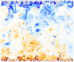



1. Introduction
Thermal convection plays an important role in a range of processes in nature and various industrial applications, where the underlying surfaces are always rough. Rayleigh–Bénard convection (RBC) is an ideal model (Bodenschatz, Pesch & Ahlers Reference Bodenschatz, Pesch and Ahlers2000; Ahlers, Grossmann & Lohse Reference Ahlers, Grossmann and Lohse2009; Chilla & Schumacher Reference Chilla and Schumacher2012) used for studying thermal convection, where a fluid confined between two horizontal plates is heated from the bottom and cooled from the top. The dynamics of RBC is governed mainly by two non-dimensional parameters, the Rayleigh number ( ${\textit {Ra}} = \beta g\,\Delta T\,H^3/\nu \alpha$) and the Prandtl number (
 ${\textit {Pr}} = \nu /\alpha$), where
 $\beta$ is the isobaric thermal expansion coefficient,
 $\Delta T=T_H-T_C$ is the temperature difference between the bottom and top plates,
 $g$ is the acceleration due to gravity,
 $H$ is the height of the fluid layer,
 $\nu$ is the kinematic viscosity, and
 $\alpha$ is the thermal diffusivity of the fluid. One of the central issues in the study of turbulent RBC is to determine the global heat transfer mechanism and scaling law that describes it. Heat transfer is quantified in terms of the non-dimensional parameter the Nusselt number
 ${\textit {Nu}}$, which gives a relative measure of the heat transfer due to convection over conduction. For the scaling law of heat transfer,
 ${\textit {Nu}}({\textit {Ra}})$ is proposed in the form
 ${\textit {Nu}} = A\,{\textit {Ra}}^\gamma$ (Grossmann & Lohse Reference Grossmann and Lohse2000). One of the main motives of ongoing research is to increase heat transfer for a given
 ${\textit {Ra}}$, which can be achieved with an increase in
 $A$,
 $\gamma$, or both.
Various heat transfer theories have been proposed in the past to quantify the heat transfer mechanism, and nearly all of them focus strongly on the dynamics in the boundary layer (BL) region. Malkus (Reference Malkus1954) assumed the marginal stability of the thermal boundary layers (TBLs) and predicted  $\gamma = 1/3$, which also suggests that heat flux is independent of
 $H$ or, in other words, top and bottom TBLs do not communicate. Kraichnan (Reference Kraichnan1962) and Spiegel (Reference Spiegel1963) predicted that at extremely large
 ${\textit {Ra}}$, BLs undergo a transition from laminar to turbulent state, which leads to a regime known as the asymptotic or ‘ultimate’ regime where
 $\gamma = 1/2$. In this regime, heat is transported ballistically with negligible resistance from the diffusivities of a fluid. Following a rigorous analysis based on the decomposition of the kinetic and thermal dissipation rates into bulk and BL contributions, Grossmann & Lohse (Reference Grossmann and Lohse2000, Reference Grossmann and Lohse2001) proposed a unifying scaling theory, where scaling laws are dependent on the
 ${\textit {Ra}}$ and
 ${\textit {Pr}}$ regimes rather than being universal ones. In this theory, the ultimate regime is also predicted as one of the regimes. But whether or not the ultimate regime exists has perplexed the scientific community for a very long time and is the most debated topic. In various experiments (He et al. Reference He, Funfshilling, Bodenschatz and Ahlers2012a,Reference He, Funfshilling, Nobach, Bodenschatz and Ahlersb; Ahlers, Bodenschatz & He Reference Ahlers, Bodenschatz and He2014), a transition to the ultimate regime has been reported at
 ${\textit {Ra}}\sim 10^{14}$, while other works (Niemela et al. Reference Niemela, Skrbek, Sreenivasan and Donnelly2000; Niemela & Sreenivasan Reference Niemela and Sreenivasan2010; Urban et al. Reference Urban, Hanzelka, Musilová, Králík, Mantia, Srnka and Skrbek2014) denied any sign of the ultimate regime. Zhu et al. (Reference Zhu, Mathai, Stevens, Verzicco and Lohse2018), through numerical investigations, also ascertained the transition to the ultimate regime at
 ${\textit {Ra}} \sim 10^{13}$. Various strategies have been used to reach the ultimate regime, from numerical studies involving periodic boundary conditions (Lohse & Toschi Reference Lohse and Toschi2003) in all directions to experimental work where radiative heating (Lepot, Aumaître & Gallet Reference Lepot, Aumaître and Gallet2018) is introduced to heat the bulk fluid directly, and thus the effect of the BLs is negated. Surface roughness is also one of the adopted strategies meant to introduce turbulence in the BLs to seek the realization of the ultimate regime and the associated
 $1/2$ scaling. Though roughness facilitates enhanced heat transport scaling, the effect is observed to be transitional (Zhu et al. Reference Zhu, Stevens, Verzicco and Lohse2017) as the classical scaling returns at a higher
 ${\textit {Ra}}$ range. The limitation is now being challenged with the introduction of multi-scale rough surfaces (Zhu et al. Reference Zhu, Stevens, Shishkina, Verzicco and Lohse2019) as opposed to simple mono-scale and periodic ones, allowing sustenance of the enhanced scaling for an even larger
 ${\textit {Ra}}$ range.
It is well established that any wall roughness becomes influential (increases heat transfer) only above a certain  ${\textit {Ra}}$ when the TBL thickness is smaller than the height of a rough surface. Enhancement of heat transfer due to rough walls may or may not lead to an increase in the scaling exponent (
 $\gamma$). Shen, Tong & Xia (Reference Shen, Tong and Xia1996) and Du & Tong (Reference Du and Tong1998) reported an increase in heat transfer but with no change in
 $\gamma$. The amplified heat transfer rate could not be attributed solely to the increase in wetted area because of the rough surfaces (Villermaux Reference Villermaux1998). Later, in various experiments (Ciliberto & Laroche Reference Ciliberto and Laroche1999; Roche et al. Reference Roche, Castaing, Chabaud and Hébral2001; Qiu, Xia & Tong Reference Qiu, Xia and Tong2005), an enhanced scaling exponent
 $\gamma$ was observed. Xie & Xia (Reference Xie and Xia2017) investigated experimentally the effect of periodically distributed pyramid-shaped roughness in a cylindrical container for
 $7.5\times 10^7 \leq {\textit {Ra}} \leq 1.31 \times 10^{11}$ with
 ${\textit {Pr}}$ ranging from 3.57 to 23.34. The roughness aspect ratio, defined as the ratio of the height of a roughness element to its base width, was varied from
 $0.5$ to
 $4$, and the obtained
 ${\textit {Nu}}({\textit {Ra}})$ scaling was classified into three regimes. In regime I, the
 ${\textit {Nu}}({\textit {Ra}})$ scaling was not affected due to the rough surfaces, whereas in regimes II and III, enhanced heat transport scaling was obtained. The transition from regime I to regime II occurs with the TBL becoming thinner than the roughness height, while the transition from regime II to regime III is marked with the viscous BL being thinner than the roughness height. Roughness elements change the local dynamics of the turbulent RBC. Du & Tong (Reference Du and Tong2000) have shown that enhancement of heat transport is due to the interaction between the large-scale circulation (LSC) and secondary flow formed inside the cavities of the roughness elements. This interaction enhances the detachment of the TBL from the tips of the rough surfaces leading to an increase in plume emission. Thus the enhancement of heat transfer is due to the changed near-wall dynamics in the presence of the rough surfaces. Belkadi et al. (Reference Belkadi, Guislain, Sergent, Podvin, Chillá and Salort2020), using shadowgraph image analysis, also credited rough surfaces in enhancing plume emission.
Direct numerical simulations (DNS) also corroborate experimental findings that an increase in the  ${\textit {Nu}}$ scaling exponent is obtained in rough cells. Stringano, Pascazio & Verzicco (Reference Stringano, Pascazio and Verzicco2006) performed DNS in a cylindrical container of aspect ratio
 $\varGamma = D/H = 1/2$ with grooves on the top and bottom plates. The Rayleigh numbers covered were in the range
 $2\times 10^6\leq {\textit {Ra}} \leq 2\times 10^{11}$, with fixed
 ${\textit {Pr}}=0.7$. Above a threshold Rayleigh number, the scaling exponent
 $\gamma$ for grooved surfaces increased from 0.31 to 0.37. Various studies on rough cells indicate that the heat transport maximizes on tuning the geometry of the roughness elements via choosing suitable height and wavelength of the roughness elements. Shishkina & Wagner (Reference Shishkina and Wagner2011) performed two-dimensional (2-D) simulations with surface roughness in the form of rectangular elements on the horizontal plates. Results revealed that
 ${\textit {Nu}}$ does not solely depend on the wall surface area, and average heat flux was more for slender roughness elements when the distance between them exceeded their height. For closely spaced roughness elements, a decrease in heat transfer rate is observed as fluid becomes stagnant in the space between them. Zhang et al. (Reference Zhang, Sun, Bao and Zhou2017b) performed 2-D simulations for
 $10^7\leq {\textit {Ra}} \leq 10^{11}$ with constant
 ${\textit {Pr}} = 1$, where they varied the height of the roughness elements (
 $h$), and wavelength was kept fixed as
 $2h$. This study highlighted that beyond a critical height (
 $h_c$) of the roughness elements, enhanced heat transport is perceived. They reported that
 $h_c$ decreases with an increase in
 ${\textit {Ra}}$ as
 $h_c \sim {\textit {Ra}}^{-0.6}$, which also implies that a certain height of the roughness elements decreasing heat transfer at low
 ${\textit {Ra}}$ may enhance it at a higher
 ${\textit {Ra}}$. Thus the enhancement in heat transfer due to roughness is more pronounced at higher
 ${\textit {Ra}}$.
Toppaladoddi, Succi & Wettlaufer (Reference Toppaladoddi, Succi and Wettlaufer2017) studied 2-D RBC with sinusoidal roughness on both the horizontal plates, where the height of the roughness elements was kept fixed. For an optimum wavelength of the roughness elements,  $\gamma = 0.483$ was obtained on fitting the data in the
 $4\times 10^6 \leq {\textit {Ra}} \leq 3\times 10^{9}$ range, which was misinterpreted as the onset of the ultimate regime. Later, Zhu et al. (Reference Zhu, Stevens, Verzicco and Lohse2017) extended the above study for an even higher
 ${\textit {Ra}}$ (
 $10^8 \leq {\textit {Ra}} \leq 10^{12}$) and clarified that the regime with
 $\gamma = 1/2$ is transient, as with a further increase in
 ${\textit {Ra}}$, the classical scaling regime (
 $\gamma = 1/3$) is restored. Revival of the classical scaling regime was attributed to the strong mixing of the fluid inside the roughness cavities. The vigorous mixing led to the formation of a thin TBL, which covered the entire rough surface uniformly and perfectly mimicked an enlarged wet surface area. Zhu et al. (Reference Zhu, Stevens, Shishkina, Verzicco and Lohse2019) introduced multi-scale roughness of the sinusoidal form in 2-D RBC. The explored
 ${\textit {Ra}}$ range was
 $10^8 \leq {\textit {Ra}} \leq 10^{11}$ with constant
 ${\textit {Pr}} = 1$ for aspect ratio
 $\varGamma = L/H = 2$. With three different distinct length scales of the roughness elements, the local
 $1/2$ scaling regime was extended and the revival of the classical
 $1/3$ scaling was put off. While explaining the efficacy of the multi-scale roughness, it was hypothesized that with increasing
 ${\textit {Ra}}$, different roughness length scales perturb the TBL in order, starting from the largest (at low
 ${\textit {Ra}}$) to the smallest (at high
 ${\textit {Ra}}$). Emran & Shishkina (Reference Emran and Shishkina2020) performed three-dimensional (3-D) DNS simulations with ring-shaped obstacles in a cylindrical cell, where for an optimum height and gap between the obstacles, an increased
 $\gamma$ was observed. Recently, Toppaladoddi et al. (Reference Toppaladoddi, Wells, Doering and Wettlaufer2021) also reported increased
 $\gamma$ with the application of the fractal boundaries in a 2-D cell. To the best of our knowledge, the effect of a complex roughness on flow dynamics has not been studied extensively. In the present work, a complex random roughness that incorporates multiple length scales, contrary to three scales employed by Zhu et al. (Reference Zhu, Stevens, Shishkina, Verzicco and Lohse2019), is introduced in a 2-D rectangular convection cell to emulate real flow-like situations with an objective to unravel the heat transport mechanism and the associated flow dynamics in different regions of the convection cell. The reason for choosing 2-D simulations is the luxury of exploring the flow physics at a higher
 ${\textit {Ra}}$ range, which is computationally prohibitive for 3-D simulations (Zhu et al. Reference Zhu, Stevens, Verzicco and Lohse2017, Reference Zhu, Stevens, Shishkina, Verzicco and Lohse2019).
The remainder of the paper is organized as follows. In § 2, the problem is set up and the numerical method is discussed. Also, results with the present numerical set-up are compared with the previous roughness study (Zhu et al. Reference Zhu, Stevens, Verzicco and Lohse2017) for sinusoidal roughness. Section 3 is the results and discussion section, which is composed of six subsections starting with § 3.1 where heat transport phenomena and their evolution with  ${\textit {Ra}}$ are explored, with a focus on the roles played by different roughness elements in enhancing heat transport. Also, comparisons are drawn with the smooth RBC to distinguish the heat transfer mechanisms. Next, in § 3.2, plume and background regions are studied to highlight the increased presence of plumes with rough surfaces, followed by §§ 3.3 and 3.4, where near-wall and bulk dynamics, respectively, are taken up to investigate closely the altered flow dynamics. Subsection 3.5 is presented with arguments in favour of the scaling proposed by Bolgiano (Reference Bolgiano1959) and Obukhov (Reference Obukhov1959) for the observed velocity and temperature fluctuations in the bulk region, and in § 3.6, orthogonal decomposition of the flow field is carried out to observe the dominant flow structures and their contributions in heat transfer. Finally, the results obtained in the present study are summarized in § 4.
2. Numerical details
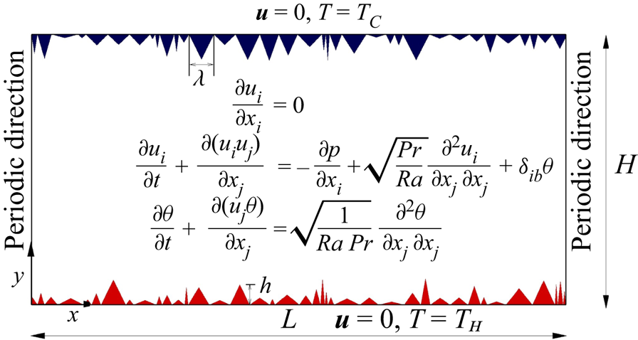
For incompressible buoyancy-driven flows, the set of non-dimensional transport equations is obtained by invoking the Boussinesq approximation. Figure 1 shows the equations, applied boundary conditions and detailed roughness geometry used in the present investigation. Here,  $u_i = (u, v)$ is the velocity in Cartesian direction
 $x_i = (x, y)$,
 $\theta = (T - T_C)/(T_H-T_C)$ is the non-dimensional temperature,
 $p$ is the pressure,
 $b$ is the buoyancy direction, and
 $\delta$ is the Kronecker delta. Reference scales for length, velocity, temperature and time are vertical height
 $H$, free-fall velocity
 $\sqrt {\beta g\,\Delta T\,H}$,
 $\Delta T = T_H - T_C$, and
 $(H/\beta g\,\Delta T)^{1/2}$, respectively. All simulations are carried out in a 2-D rectangular cell of aspect ratio
 $\varGamma = L/H = 2$ with air as the working fluid (
 ${\textit {Pr}} = 0.7$) for
 $10^8 \leq {\textit {Ra}} \leq 10^{11}$. Top and bottom horizontal walls are endowed with rough surfaces, consisting of random triangular elements with no-slip velocity and isothermal temperature boundary conditions imposed on them, while the lateral walls are smooth and periodic. Amplitude (
 $h$) and wavelength (
 $\lambda$) of the roughness elements are assigned using the standard random number generator available in the Intel Fortran 90 platform. The library functions ‘random seed’ and ‘random number’ are invoked for the assignment. Both
 $h$ and
 $\lambda$ are set to vary independently, and they are scaled between 1 and 10 % of the cell height, which implies that the height and base of the elements may assume any value ranging from 0.01 to 0.1. The creation of an isosceles triangular element can be accomplished easily once the values of
 $h$ and
 $\lambda$ are obtained from the random number generator. In the same fashion, the roughness elements of different combinations of
 $h$ and
 $\lambda$ are created to fill the top and bottom isothermal horizontal plates. The spectrum of truly random distribution is likely to contain all possible numbers. However, owing to the finite axial length, the number of elements that can be accommodated is also finite. Though the base and height of an element are chosen arbitrarily, a finite number of such elements limits all possible
 $(\lambda,h)$ combinations. Thus the present roughness set-up is multi-scale, but it is random to only a limited extent. See Appendix A.5 for more details about the distribution followed by
 $h$ and
 $\lambda$. Note that in order to express
 ${\textit {Ra}}$ for the rough cases, the effective height of the cell, as described by Zhu et al. (Reference Zhu, Stevens, Shishkina, Verzicco and Lohse2019), is considered as the characteristic length scale.
Schematic showing a 2-D rectangular convection cell with random triangular roughness elements at the top and bottom plates. Here,  $h$ and
 $\lambda$ denote height and width (wavelength) of the roughness elements, respectively.

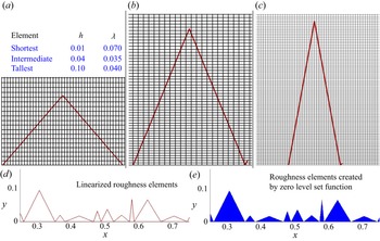
The governing equations are solved using a non-staggered finite volume approach in conjunction with a diffuse interface immersed boundary method (DIIBM) (De Reference De2018) to handle the roughness elements. The boundary of the object (roughened plates) is first linearized in order to ascertain its relation to the computing cells surrounding it. Computing cells are classified into fluid or body cells based on the volume fraction, which is the fraction of a computing cell lying inside an object. Since the DIIBM does not essentially demarcate the body surface from the fluid region, a universal momentum equation, which smoothly blends the Navier–Stokes equations with the velocity boundary conditions, is solved in the entire physical domain regardless of whether the computing cell belongs to fluid or solid body. Buoyancy, pressure and diffusive terms in the momentum equation are handled using the second-order Crank–Nicolson scheme, while the nonlinear convective term is approximated using the Adams–Bashforth scheme. A two-step predictor-corrector technique is employed in the solver. In the first step, the provisional velocity field is calculated using the known pressure field, and in the second step, it is corrected by solving the pressure Poisson equation, which enforces mass balance indirectly. All the resulting sparse linear systems are solved using the BiCGSTAB technique preconditioned by a highly scalable block diagonal version of the modified strongly implicit (MSI) procedure. The solver used for the computations is parallelized with standard MPI libraries to speed up the calculations. For further details of the numerical technique, see Peter & De (Reference Peter and De2016) and De, Eswaran & Mishra (Reference De, Eswaran and Mishra2018).
A grid that is uniform in  $x$ and non-uniform in
 $y$ is employed such that the regions close to rough surfaces are resolved sufficiently. At a particular
 ${\textit {Ra}}$, maximum grid spacing in
 $y$ (
 $\Delta y_{max}$) is kept comparable to the global Kolmogorov length scale (
 $\eta$) estimated as
 ${\textit {Pr}}^{1/2}({\textit {Ra}}\,{\textit {Nu}})^{-1/4}$ such that
 $\Delta y_{max} /\eta$ is always less than
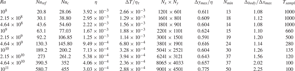
 $0.8$. Triangular elements are resolved in such a way that their resolution is comparable to that of the grid. Further, at least thirteen computing cells in the vertical
 $y$ direction are kept inside the smallest roughness element (
 $h=0.01$). See table 1 for details of the simulation parameters. The time increment is chosen in such a way that it is smaller than the Kolmogorov time scale (
 $\eta _{\tau }$), and the maximum Courant number is always less than 0.2. For simulation runs, the flow field of a lower
 ${\textit {Ra}}$ is linearly interpolated and subsequently used as the initial condition for the next higher
 ${\textit {Ra}}$ case to speed up attainment of the statistically stationary state after which data are sampled. Details of the data sampling duration (
 $T_{sampl}$) are listed in table 1. While for the highest
 ${\textit {Ra}}$, the sampling time is kept as large as 1000 free-fall time units to realize the fully developed turbulent state, a sampling of 100 units is found adequate for the highly turbulent highest
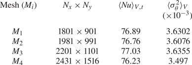
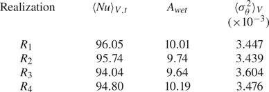
 ${\textit {Ra}}$ case, which also involves a very high spatial resolution. Further details about the code validation, mesh convergence, different flow realizations and the implemented DIIBM are provided in Appendix A.
Details of simulation parameters starting from the left:  ${\textit {Ra}}$ is the Rayleigh number;
 ${\textit {Nu}}_{ref}$ is the reference Nusselt number taken from Zhu et al. (Reference Zhu, Stevens, Shishkina, Verzicco and Lohse2019);
 ${\textit {Nu}}_c$ is the calculated Nusselt number;
 $\eta$ is the Kolmogorov length scale estimated as
 $\eta \approx {\textit {Pr}}^{1/2}/({\textit {Ra}}\,{\textit {Nu}})^{1/4}$;
 $\Delta T/\eta _{\tau }$ is the ratio of time step to Kolmogorov time scale
 $\eta _{\tau }=\sqrt {{\textit {Pr}}/({\textit {Nu}}-1)}$;
 $N_x$ and
 $N_y$ are the grid resolutions in the
 $x$ and
 $y$ directions, respectively;
 $\Delta y_{max}/\eta$ is the ratio of maximum grid spacing in the
 $y$ direction to the Kolmogorov length scale
 $\eta$;
 $N_{min}$ represents the number of grid points inside the smallest roughness element in the
 $y$ direction;
 $\Delta _{body}/\Delta x_{max}$ is the ratio of resolution of the roughness elements to the maximum grid spacing in the
 $x$ direction;
 $T_{sampl}$ represents the data sampling duration.

3. Results and discussions
In the following discussions, different types of ensemble averages of a random variable  $\phi (x,y,t)$ are represented as follows:
 $\langle \phi \rangle _{t}$ represents the time average,
 $\langle \phi \rangle _{V,t}$ is the volume and time average, and
 $\langle \phi \rangle _{A,t}$ is the horizontal line and time average.
3.1. Heat transport mechanism
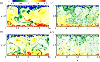
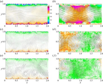
One of the key challenges in turbulent RBC is to understand the heat transport phenomena, where thermal plumes and LSC serve as thermal carriers in transporting heat from the bottom heated plate to the top cooled plate. With the introduction of rough surfaces, flow dynamics in a thermal convection cell is believed to be altered, which often favours augmented heat transport at a sufficiently high thermal forcing. In figure 2, snapshots of the instantaneous temperature field are shown for  ${\textit {Ra}}$ ranging from
 $10^8$ to
 $10^{11}$, where evolution of the flow structures with increasing
 ${\textit {Ra}}$ can be observed. At the lowest
 ${\textit {Ra}} =10^8$, flow inside the cavities (formed between the roughness elements) is still viscosity-dominated, which is evident from the entrapment of fluid inside the cavities, and thus a thick TBL is seen to form, as a result of which, significant enhancement in heat transport is not achieved. The major contribution to the plume emission comes from the taller roughness elements as shorter elements are embedded inside the TBL and are unable to perturb the BL region. With the increase in
 ${\textit {Ra}}$, fluid trapped inside the cavities becomes accessible to the bulk flow and is eventually washed away, resulting in better mixing and a thin TBL. As the height of the smaller elements becomes comparable to TBL thickness, they start to contribute to plume emission. At the highest
 ${\textit {Ra}}=10^{11}$, the flow is highly turbulent and homogeneous with the emergence of very fine flow structures. Large-scale diffuse structures are seen to carry mainly heat at the smaller
 ${\textit {Ra}}$. This causes interdependency between the plumes, which often deters heat transfer enhancement. However, as flow structures become finer and intense, localized effects become important, and the plume emission process is triggered even at the sloping sides. As nucleation sites multiply, heat transport also magnifies.
Snapshots of instantaneous temperature field for (a)  ${\textit {Ra}}=10^8$, (b)
 ${\textit {Ra}}=10^9$, (c)
 ${\textit {Ra}}=2.15 \times 10^{10}$, and (d)
 ${\textit {Ra}}=10^{11}$.

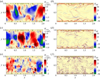
To further elucidate the heat transport process, local instantaneous heat flux is decomposed into the contributions from diffusion and convection, defined as
 \begin{align} {\textit{Nu}}&=\underbrace{\sqrt{{\textit{Ra}}\,{\textit{Pr}}}\,(v\theta)}_{convection } +\underbrace{(-\partial_y \theta)}_{diffusion}\nonumber\\ &=H_{conv}+H_{diff}, \end{align}
which are shown in figure 3. As convective heat flux ( $H_{conv}$) is associated with the product
 $v\theta$, it represents the transfer of heat by the vertical component of the fluid velocity. Here,
 $H_{conv}$ is positive for the ascent of the fluid (
 $v>0$), while it is negative for the descent (
 $v<0$). Clearly, a larger magnitude of
 $v\theta$ corresponds to a stronger convective effect. Diffusive heat flux (
 $H_{diff}$), on the other hand, takes into account the heat transfer due to vertical temperature gradient,
 $\partial _y\theta$. In the expression for
 $H_{diff}$,
 $\partial _y\theta$ is preceded by a negative sign, which signifies that the diffusive contribution of the heat flux is positive in the direction of buoyancy. Near the BL regions, the diffusive contribution is predominant owing to the strong temperature gradient in comparison to the bulk region. Also, plumes detaching from roughness elements exhibit high
 $H_{diff}$ at their interfaces, which distinguishes them from the rest of the fluid. In view of this, it can be seen that at the lowest
 ${\textit {Ra}}=10^8$, there are fewer plume-emitting spots, while at the highest
 ${\textit {Ra}}=10^{11}$, we observe significantly increased plume emission sites with visibly finer plumes. As for convective contributions, they are expected to increase with increasing
 ${\textit {Ra}}$ (prefactor
 $\sqrt {{\textit {Ra}}\,{\textit {Pr}}}$ of
 $H_{conv}$ increases with
 ${\textit {Ra}}$) and the same is evident in figure 3. At the highest
 ${\textit {Ra}}=10^{11}$, maximum convective heat flux is of the order of
 $10^5$, which is nearly two orders of magnitude higher than that at the lowest
 ${\textit {Ra}}=10^8$. Plume regions are identified clearly by high
 $H_{conv}$. Thus at all
 ${\textit {Ra}}$, plumes are observed to be the most potent coherent structures in enhancing the heat transfer. Interestingly, the shape of these regions does not change even at the highest
 ${\textit {Ra}}$. This indicates clearly that though visibly plumes become finer at higher
 ${\textit {Ra}}$, their spread – and thus the convective effects brought about by them – increases in magnitude while they control the heat transfer away from the walls. Note that
 $H_{diff}$ contributions are trivial in comparison to
 $H_{conv}$ in the flow field, though high values of the former in the vicinity of the roughness elements show the signatures of the plumes.
Instantaneous local convective and diffusive heat flux fields are shown for  ${\textit {Ra}}=10^8$ (a,b),
 ${\textit {Ra}}=10^9$ (c,d), and
 ${\textit {Ra}}=10^{11}$ (e, f). Here,
 $H_{conv}=\sqrt {{\textit {Ra}}\,{\textit {Pr}}}\, v\theta$ is the convective flux, while
 $H_{diff}=-\partial _y\theta$ is the diffusive flux. Note that the data sets correspond to the same instances as in figure 2.

Next, we analyse how the global heat flux represented by  $\langle {\textit {Nu}}\rangle _{V,t}=\sqrt {{\textit {Ra}}\, {\textit {Pr}}}\langle v\theta \rangle _{V,t} - $
 $ \langle \partial _y\theta \rangle _{V,t}$ evolves with increasing
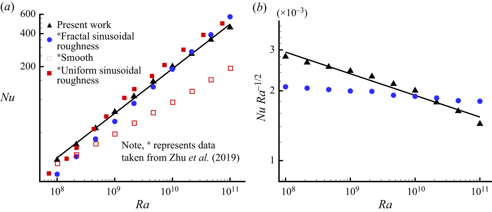
 ${\textit {Ra}}$, as shown in figure 4. Using the least-squares fit, a heat transport scaling relation is obtained as
 ${\textit {Nu}}= 0.016\,{\textit {Ra}}^{0.41}$, which highlights the attainment of the augmented scaling (Zhu et al. Reference Zhu, Stevens, Verzicco and Lohse2017). For comparison, Nusselt numbers reported by Zhu et al. (Reference Zhu, Stevens, Shishkina, Verzicco and Lohse2019) for the smooth wall, mono-scale and fractal-like sinusoidal roughness are also shown. Least-squares fitting to their data for fractal-like roughness revealed the scaling relation as
 ${\textit {Nu}}= 0.003\,{\textit {Ra}}^{0.48}$. It can be observed that for the first two decades,
 $10^8 \le {\textit {Ra}} \le 10^{10}$, the present roughness configuration yields higher
 ${\textit {Nu}}$, while in the last decade,
 $10^{10}<{\textit {Ra}}\le 10^{11}$, it is comparable with the reference
 ${\textit {Nu}}$. Figure 4(b) highlights clearly the difference in the two scalings, where
 ${\textit {Nu}}\,{\textit {Ra}}^{-1/2}$ is plotted against
 ${\textit {Ra}}$. The larger intercept on the
 ${\textit {Nu}}\,{\textit {Ra}}^{-1/2}$ axis for the present work signifies a greater prefactor, while comparatively flatter fitting for the reference data implies that the exponent is closer to
 $1/2$. Note that Zhu et al. (Reference Zhu, Stevens, Shishkina, Verzicco and Lohse2019) chose the optimized parameters (
 $h/\lambda =1$) for their roughness configuration to realize the maximum possible scaling exponent in comparison to other combinations of the amplitude and wavelength of the roughness elements. However, in the present work with random roughness, there is no preference for any particular combination of the amplitude and wavelength of the roughness elements. The above argument highlights the possible reason for the difference in the scaling exponents. Nevertheless, this study corroborates the finding of Zhu et al. (Reference Zhu, Stevens, Shishkina, Verzicco and Lohse2019) that multi-scale roughness extends the
 ${\textit {Ra}}$ range up to which augmented scaling (
 $1/3 < \gamma \leq 1/2$) is realized. Also, it can be inferred that use of an optimized and simplified roughness may overpredict the scaling exponent as opposed to its realistic version where all possible responses of the roughness elements are present.
(a) The  ${\textit {Nu}}({\textit {Ra}})$ scaling is shown for three decades of
 ${\textit {Ra}}$ (
 $10^8\le {\textit {Ra}} \le 10^{11}$). For comparison, data for smooth, mono-scale and fractal-like sinusoidal roughness taken from Zhu et al. (Reference Zhu, Stevens, Shishkina, Verzicco and Lohse2019) are also shown. Using least-squares fitting, the scaling relations for multi-scale cases are obtained as
 ${\textit {Nu}}=0.016\,{\textit {Ra}}^{0.41}$ (present work), and
 ${\textit {Nu}}_{ref}= 0.003\,{\textit {Ra}}^{0.48}$. (b) Compensated
 ${\textit {Nu}}\,{\textit {Ra}}^{-1/2}$ plots for the multi-scale cases.

Next, we delve into the production and dissipation of the turbulent kinetic energy (TKE) to see how they fare for the rough surfaces. The dynamical equation for the TKE budget is obtained by contracting the equation of velocity fluctuation and then effecting a suitable ensemble average (represented by an overbar). The resulting TKE budget is
 $$\begin{gather} \underbrace{\frac{\partial}{\partial t}\left(\frac{1}{2}\overline{u^\prime_iu^\prime_i}\right) +U_j\,\frac{\partial}{\partial x_j}\left(\frac{1}{2}\overline{u_i^\prime u_i^\prime}\right)}_{A_K}= \underbrace{-\overline{u_i^\prime u_j^\prime}\,S_{ij}}_{P_S}+\underbrace{ \overline{u_i^\prime \theta^\prime}\,\delta_{iy}}_{P_B}-\underbrace{2\sqrt{\frac{{\textit{Pr}}}{{\textit{Ra}}}}\,\overline{s_{ij}^\prime s_{ij}^\prime}}_\epsilon\nonumber\\ -\underbrace {\frac{\partial}{\partial x_j}\left(\overline{u_j^\prime p^\prime}+\frac{1}{2}\overline{u_i^\prime u_i^\prime u_j^\prime}-2\sqrt{\frac{{\textit{Pr}}}{{\textit{Ra}}}}\, \overline{u_i^\prime s_{ij}^\prime}\right)}_{T_K}, \end{gather}$$
where the terms (left to right) are cast as advection  $A_K$, shear production
 $P_S$, buoyancy production
 $P_B$, dissipation
 $\epsilon$, and transport
 $T_K$ of
 $1/2\overline {u^\prime _iu^\prime _i}$. Production terms
 $P_S$ and
 $P_B$ feed energy to the system to sustain turbulence, while
 $\epsilon$ denotes dissipation of energy due to viscous forces in action at small scales. In buoyancy-driven flows,
 $P_B$ is expected to be higher than
 $P_S$ as the flow is driven by thermo-convective instabilities. An important insight about thermal convection is revealed when global contributions of the different terms in the TKE budget are considered. The volume–time-averaged contributions of
 $A_K$,
 $T_K$ and
 $P_S$ being negligible result in an exact balance between global buoyancy production (
 $P_B$) and turbulent dissipation (
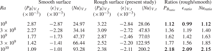
 $\epsilon$). In table 2, a direct comparison is made between the present rough case and the smooth surface case (Chand et al. Reference Chand, Sharma, Sharma and De2019) for volume–time-averaged
 $P_B$,
 $\epsilon$ and the Nusselt number. Note that in the present roughness configuration, there is a slight digression from the expected balance between the global
 $P_B$ and
 $\epsilon$. The exact reasons contributing to the deviation were not understood. However, it is suspected that the nature of the roughness terrain plays a large role in determining how well the velocity gradients at the interface of the fluid and rough surfaces are calculated. The complex roughness terrain employed in the present study might be responsible for the observed slight imbalance. From table 2, it can be observed that both
 $\langle P_B \rangle _{V,t}$ and
 $\langle \epsilon \rangle _{V,t}$ are higher for the present study. At the lowest
 ${\textit {Ra}}$,
 $P_B$,
 $\epsilon$ and
 ${\textit {Nu}}$ are comparable with their smooth surface counterparts, implying that no change is induced by the roughness. However, at
 ${\textit {Ra}}=10^{10}$, both
 $\langle P_B \rangle _{V,t}$ and
 $\langle \epsilon \rangle _{V,t}$ are approximately two times higher (highlighted in bold) than their smooth surface counterparts. Increased
 $P_B$ is a clear indicator of the enhanced heat transport, which highlights the usefulness of employing roughness in RBC. It is important to address how roughness contributes to the enhanced buoyancy production. Zhang et al. (Reference Zhang, Huang, Jiang, Liu, Lu, Qiu and Zhou2017a) reported that rising and falling plumes exhibit high turbulent heat flux (
 $v^\prime \theta ^\prime$) as well as high turbulent dissipation rates. Along the same lines we have shown above how plume emission multiplies at higher
 ${\textit {Ra}}$. Thus we may reason that the augmentation of plume emission frequency is the cause of enhanced heat transport at higher
 ${\textit {Ra}}$ that appears through an increased buoyancy production.
The effect of employing rough surfaces is highlighted by drawing a direct comparison with the smooth surface case (Chand et al. Reference Chand, Sharma, Sharma and De2019) for volume–time-averaged turbulent buoyancy production ( $P_B$), dissipation (
 $\epsilon$) and the Nusselt number (
 ${\textit {Nu}}$).

3.2. Plume statistics
Thermal plume is the coherent structure that contributes substantially in the heat transport process. A number of visualization studies (Zhou, Sun & Xia Reference Zhou, Sun and Xia2007; Shishkina & Wagner Reference Shishkina and Wagner2008; Zhou & Xia Reference Zhou and Xia2010) have identified thermal plumes as either mushroom or sheet-like structures. Plumes are formed near the isothermal walls from where they drift to the bulk region while carrying heat with them. To detect plumes from the turbulent background, the threshold technique suggested by Emran & Schumacher (Reference Emran and Schumacher2012), where strong positive correlation between the vertical velocity ( $v^\prime$) and temperature (
 $\theta ^\prime$) fluctuations indicates plume-dominated regions, is implemented in the present work. Temperature fluctuation is defined as
 $\theta ^\prime (\boldsymbol {x},t)= \theta (\boldsymbol {x},t)-\langle \theta (\boldsymbol {x})\rangle _{A,t}$, while owing to
 $\langle v\rangle _{A,t}=0$, velocity fluctuation is taken as
 $v^\prime (x,t)=v(x,t)$, where
 $\langle \rangle _{A,t}$ denotes averaging over horizontal plane and time. In the present study, decomposition of the whole domain, based on whether a region is dominated by plumes or background, is carried out using the criteria
 \begin{equation} \left. \begin{aligned} V_{pl} & =\boldsymbol{x}\in V : v^\prime\theta^\prime/\varGamma^\prime > \delta, \\ V_{bg} & =\boldsymbol{x}\in V : v^\prime\theta^\prime/\varGamma^\prime \le \delta. \end{aligned} \right\} \end{equation}
Here,  $V_{pl}$ and
 $V_{bg}$ are the volume fractions of the plume- and background-dominated regions, respectively,
 $\varGamma ^\prime$ represents instantaneous global maximum of
 $v^\prime \theta ^\prime$, and
 $\delta$ is a free parameter that imposes the threshold criterion. The idea behind using different threshold values is to observe cut-off dependency for plumes, if any. In the present work, four threshold values,
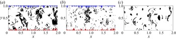
 $\delta = 0.1\,\%$, 1 %, 5 % and 10 %, are used. In figure 5, instantaneously extracted plumes and background regions using the above criteria with
 $\delta =5\,\%$ are shown for
 ${\textit {Ra}} =10^{10}$ and
 $10^{11}$ along with a case for the smooth surface at
 ${\textit {Ra}}=10^{10}$. Plume regions are seen clearly to expand with the introduction of roughness. While traces of remnant plumes are found near the roughened surface, they become stretched and scattered at higher
 ${\textit {Ra}}$. Dependency of the volume fractions for plume and background regions on
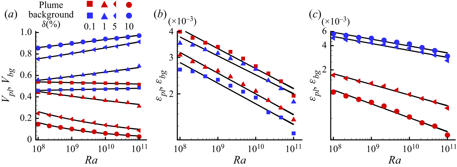
 ${\textit {Ra}}$ for different threshold (
 $\delta$) values is shown in figure 6(a). It can be observed that irrespective of
 $\delta$, a decreasing trend of plume volume fractions is obtained with
 ${\textit {Ra}}$, while the background fractions compensate it. Clearly, a larger threshold turns out to be a stricter condition for a region to qualify as a plume.
Plume (black) and background (white) regions are identified using a threshold  $\delta =5\,\%$ for (a)
 ${\textit {Ra}} =10^{10}$, (b)
 ${\textit {Ra}} =10^{11}$, and (c)
 ${\textit {Ra}}=10^{10}$ for the plane surface case. Note that (a,b) correspond to the same time instances as in figure 2.

 ${\textit {Ra}}$ and
 $\delta$ dependency of (a) volume fractions of plumes (
 $V_{pl}$) and background (
 $V_{bg}$), (b,c) dissipation rates of plumes (
 $\epsilon _{pl}$) and background (
 $\epsilon _{bg}$). Note that
 $\epsilon _{pl}$ and
 $\epsilon _{bg}$ are shown for
 $\delta =0.1$ and
 $1\,\%$ in (b), but for
 $\delta =5$ and
 $10\,\%$ in (c). Symbols in red and blue correspond to plume and background, respectively, while solid black lines represent power-law fittings.

A comparison of thermal dissipation rates,  $\epsilon _\theta =({\textit {Ra}}\,{\textit {Pr}})^{-1/2}\vert \boldsymbol {\nabla } \theta \vert ^2$, of plume (
 $\epsilon _{pl}$) and background (
 $\epsilon _{bg}$) regions, which are obtained as
 \begin{equation} \epsilon_{pl}= \left\langle \int_{V_{pl}} \epsilon_\theta(\boldsymbol{x},t)\,{\rm d}V \right\rangle_t \quad \text{and} \quad \epsilon_{bg}= \left\langle \int_{V_{bg}} \epsilon_\theta(\boldsymbol{x},t)\,{\rm d}V \right\rangle_t, \end{equation}
indicate dominant heat transfer agent in the flow. Note that  $\epsilon _{pl}$ and
 $\epsilon _{bg}$ represent total time-averaged contributions in thermal dissipation from plume- and background-dominated regions, respectively. In figures 6(b) and 6(c), the variations of
 $\epsilon _{pl}$ and
 $\epsilon _{bg}$ are shown with increasing
 ${\textit {Ra}}$. It can be observed that for all threshold (
 $\delta$) values, contributions of both
 $\epsilon _{pl}$ and
 $\epsilon _{bg}$ decline as
 ${\textit {Ra}}$ increases. Interestingly, for
 $\delta = 0.1\,\%$,
 $\epsilon _{pl}$ exceeds
 $\epsilon _{bg}$ at all
 ${\textit {Ra}}$, whereas for
 $\delta = 1\,\%$, 5 %, 10 %,
 $\epsilon _{bg}$ exceeds
 $\epsilon _{pl}$. On the other hand, at a given
 ${\textit {Ra}}$, with the increase in
 $\delta$,
 $\epsilon _{bg}$ grows while
 $\epsilon _{pl}$ decays. A larger
 $\delta$ allows larger background, which implies that
 $\epsilon _{bg}$ contributions are incorporated from larger regions. On the other hand, for plumes, a larger
 $\delta$ yields a smaller
 $V_{pl}$ and hence
 $\epsilon _{pl}$ drops.
Further, using least squares fitting, power laws of the form  $A\,{\textit {Ra}}^m$ are obtained for both volume fractions and dissipation rate contributions of plumes and background at different
 $\delta$ values. The obtained fitting parameters are shown in table 3. We observe that for all
 $\delta$,
 $m_{pl}$ is negative for
 $V_{pl}$, while
 $m_{bg}$ is positive for
 $V_{bg}$. It implies that with increase in
 ${\textit {Ra}}$, the effective region covered by plumes diminishes, which is taken up by the background. The scaling exponents for both
 $\epsilon _{pl}$ and
 $\epsilon _{bg}$ are negative, implying reduced thermal dissipation at higher
 ${\textit {Ra}}$. Note that the non-dimensional thermal dissipation rate (
 $\epsilon _\theta$) should not be confused with the dimensional one. The global dimensional thermal dissipation rate, denoted as
 $\epsilon _T= \alpha (\Delta T/H^2)\,{\textit {Nu}}$, augments with increasing
 ${\textit {Ra}}$ owing to the elevated
 $\Delta T$ and
 ${\textit {Nu}}$. However, the former obeys the relation
 $\langle \epsilon _\theta \rangle _V= \langle {\textit {Nu}} \rangle _V/\sqrt {{\textit {Ra}}\,{\textit {Pr}}}$, which explains the observed diminution of net thermal dissipation rate (
 $\epsilon _{pl}+ \epsilon _{bg}$) on amplification of the thermal forcing. For
 $\delta =0.1\,\%$, the scaling exponents for volume fractions are very low, indicating negligible variation of the volumes of plumes and background with increasing
 ${\textit {Ra}}$, which is also evident from figure 6(a). It can be observed that with increase in
 $\delta$, the scaling exponents for both
 $V_{pl}$ and
 $\epsilon _{pl}$ increase in absolute sense, while for
 $V_{bg}$ and
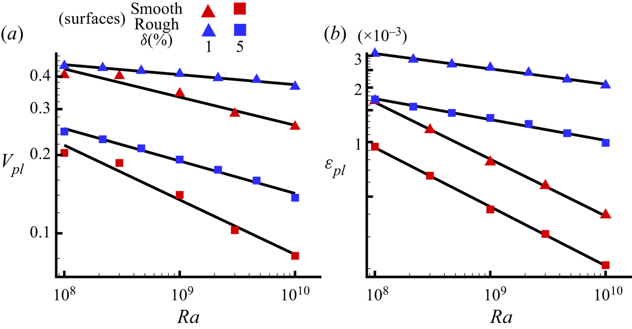
 $\epsilon _{bg}$, they appear to be more stable. Further, to explain how roughness alters plume regions, variation of
 $V_{pl}$ and
 $\epsilon _{pl}$ with
 ${\textit {Ra}}$ is compared with the smooth surface case (Chand et al. Reference Chand, Sharma, Sharma and De2019) for
 $\delta =1\,\%$ and
 $5\,\%$ in figure 7. It is clear that irrespective of
 $\delta$, both
 $V_{pl}$ and
 $\epsilon _{pl}$ are higher for the roughened surface with slower decay over increasing
 ${\textit {Ra}}$. This re-emphasizes the effectiveness of rough surfaces in enhancing the plume emission process. Also, a slower decay rate of
 $V_{pl}$ and
 $\epsilon _{pl}$ indicate that the effect of roughness is sustained even at higher
 ${\textit {Ra}}$. Though at higher thresholds, plume regions follow a near identical behaviour, the dissipation contribution continues to dominate for the rough surface configuration.
A comparison is made for the variation of (a)  $V_{pl}$ and (b)
 $\epsilon _{pl}$ with
 ${\textit {Ra}}$ between rough and smooth surfaces for
 $\delta =1$ and
 $5\,\%$. Symbols in red and blue represent data for smooth (Chand et al. Reference Chand, Sharma, Sharma and De2019) and present rough surfaces, respectively, and solid black lines represent power-law fittings.

Prefactor and exponent of the power-law fit,  $A\,{\textit {Ra}}^m$, for the volume fractions and dissipation contributions of the plume and background at different thresholds.

3.3. Near-wall dynamics
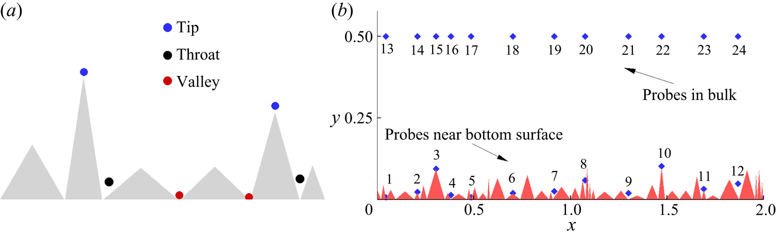
Rough surfaces significantly alter the BL dynamics, which is responsible for the augmented heat flux above a threshold  ${\textit {Ra}}$. The ability of a rough surface to facilitate extra plume generation spots is its biggest asset in influencing flow structures and dynamics. In smooth surfaces, plume eruption is driven purely by buoyancy, whereas for rough surfaces, sharp edges promote flow separation and act as the active source of plume emission (Stringano et al. Reference Stringano, Pascazio and Verzicco2006). Three types of localized regions with distinct flow features can be associated with a rough surface: above the tips, between two roughness elements (throat), and the lower point between them (valley). These regions are shown schematically in figure 8(a).
(a) Schematic diagram showing tip, throat and valley regions associated with a rough surface. (b) Location of numerical probes chosen in the vicinity of the bottom rough surface, and bulk region shown in a magnified view.

The region above the tips of the roughness elements (especially sharp ones) records high heat flux due to frequent emission of plumes, whereas the throat and cavity regions exhibit the lowest heat flux due to immobility of the trapped fluid. Motion of fluid inside the cavities is enhanced with the increase in  ${\textit {Ra}}$, and eventually the fluid becomes accessible to the bulk flow. Note that if the cavity region is too closely packed, then fluid remains struck at even higher thermal forcing (
 ${\textit {Ra}}$). To study flow dynamics effectively in the near-wall and bulk region, we have considered a total of 24 probes, half near the bottom rough surface and rest in the bulk region, as shown in figure 8(b). At the probes, time series data are recorded at a non-dimensional sampling rate of 100 units (after every
 $\Delta t =10^{-2}$).
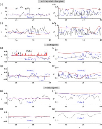
The transition of the flow states with increasing  ${\textit {Ra}}$ in the throat and tip regions can be identified using the temperature and velocity fluctuations. In figure 9, time series of vertical velocity and temperature are shown for regions near the bottom rough surface for a small window of 5 time units at three different
 ${\textit {Ra}}$ values:
 $10^8$,
 $10^{10}$ and
 $10^{11}$. At the lowest
 ${\textit {Ra}}=10^8$, we observe that both temperature and velocity fluctuations are minimum, with low vertical velocity and high mean temperature for both the tip and throat regions. This indicates essentially that the flow is nearly stagnant near the rough surface. With an increase in thermal forcing, the fluctuations increase for both the regions as bulk fluid approaches near-wall regions more effectively. Also, note that in general, both vertical velocity and temperature show larger fluctuations near the tips than in throat regions at all
 ${\textit {Ra}}$ explored, which suggests that the major source of plume emission is the tip area of the roughness elements. At one extreme, deep down the throat, large-scale inhomogeneity is evident as circulating fluid cannot reach there (see figures 9g,h). On the other extreme, near the tip of taller roughness, large oscillations are recorded owing to the interaction between newly formed plumes and large-scale rolls (see figures 9c,d). Greater mixing at the higher
 ${\textit {Ra}}$ is seen clearly through large fluctuations in vertical velocity with lower mean temperature. Thus different relative locations near the wall do not contribute to plume emission and mixing with the same intensity. It indicates varied responses of the elements at different
 ${\textit {Ra}}$ owing to their relatively distinct geometric features that occur essentially on a random surface texture.
Time series of vertical velocity (a,c,e,g,i,k) and temperature (b,d, f,h, j,l) recorded from probes placed near the bottom rough surface are shown at  ${\textit {Ra}}=10^8$,
 $10^{10}$ and
 $10^{11}$ for a small window of 5 time units. Locations of the probes (magnified view) are shown in the inset of (e).

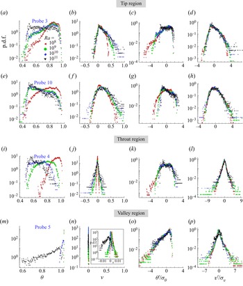
In figure 10, p.d.f.s (probability density functions) of temperature and vertical velocity, computed from the above signals, are shown in panels (a–h), and for their normalized fluctuations in panels (i–p). Note that to normalize the fluctuations, their root-mean-square (r.m.s.) values are used; for a quantity  $\phi$, this is defined as
 $\sigma _\phi ^2=\overline {\phi (t)^2}-(\bar {\phi })^2$, where an overbar denotes temporal average. From temperature p.d.f.s, it can be observed that in general, at the lowest
 ${\textit {Ra}}=10^8$, higher mean temperature (especially in throat region) is expected as peaks of the temperature p.d.f.s are skewed towards high temperature. However, with an increase in
 ${\textit {Ra}}$, there is increased probability of the lower temperature readings, and at the highest
 ${\textit {Ra}}=10^{11}$, the peaks are skewed towards the lower temperature. This also hints that at lower
 ${\textit {Ra}}$, either plume emission frequency is lower or fluid is stuck. On the other hand, at higher
 ${\textit {Ra}}$, hot plumes are emitted frequently and cold fluid rushes towards the plume-emitting spots, which explains the lower mean temperature. P.d.f.s of the normalized temperature fluctuations are seen to collapse onto one another in the core, while the tails show deviation. However, the p.d.f.s have overall different shapes for different regions, implying that temperature fluctuations are influenced locally by the roughness elements.
P.d.f.s of (a,e,i,m)  $\theta$, (b, f, j,n)
 $v$, (c,g,k,o)
 $\theta ^\prime /\sigma _\theta$, and (d,h,l,p)
 $v^\prime /\sigma _v$, for probes placed near the bottom plate at different
 ${\textit {Ra}}$. Note that each row represents the data for a particular probe; the inset in (n) shows the magnified view. See figure 8(b) for the locations of the probes.

Vertical velocity p.d.f.s being narrower at the lowest  ${\textit {Ra}} = 10^8$ clearly signify immobility of the fluid. However, with the increased
 ${\textit {Ra}}$, occurrence of events with large vertical velocity is augmented. The p.d.f.s for the tip regions have longer positive tails that extend further with increase in
 ${\textit {Ra}}$, whereas in the throat regions, they are symmetric about the zero mean. Also, they exhibit nearly equal affinity for both positive and negative vertical velocity in the throat regions, such that the maximum absolute
 $v$ is less than is observed in the tip regions. Peak regions that are surrounded by the roughness of different aspect ratio show clearly different flow behaviour. Though probes 3 and 10 are closer to the bulk, the slender one (probe 10) exhibits a near-symmetric Gaussian distribution for
 $v$, while at location 3, no extreme events for
 $v<0$ are recorded. This again indicates the varied response of the peaks to the nearest large-scale roll. Similarly, different cavity regions evolve differently with
 ${\textit {Ra}}$. For instance, probes 4 and 5 exhibit totally contrasting p.d.f.s for both
 $\theta$ and
 $v$. The fluid region depicted by probe 5 is too closely packed between the neighbouring elements, such that it is inaccessible to the bulk flow even at a higher
 ${\textit {Ra}}$, whereas probe 4 is accessible to the bulk flow at higher
 ${\textit {Ra}}$. Also, the role played by the tip regions in emitting plumes is highlighted from the p.d.f.s of the vertical velocity exhibiting a higher probability for the positive fluctuations. Thus we show that a randomly distributed roughness has a varied influence on the flow dynamics, and it cannot be characterized unilaterally.
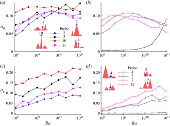
Use of rough surfaces is desired to yield enhancement in heat transport that is not achieved easily at a lower  ${\textit {Ra}}$. Improvement of the plume-emission process is reflected in the increased temperature and vertical velocity fluctuations. In figure 11, r.m.s. values of temperature and vertical velocity fluctuations, denoted by
 $\sigma _\theta$ and
 $\sigma _v$, respectively, are shown for the throat and tip regions in the explored
 ${\textit {Ra}}$ range. It can be observed that in general,
 $\sigma _\theta$ and
 $\sigma _v$ are higher near the tips. While velocity fluctuation is seen to increase monotonically, temperature fluctuation peaks at an intermediate
 ${\textit {Ra}}$ (
 $\approx 2.15\times 10^9$) followed by a drop at a higher
 ${\textit {Ra}}$. The reason for the decrease of
 $\sigma _\theta$ in throats is attributed to the effective bulk–BL interaction where a nearly homogeneous bulk fluid is now accessing and mixing well with the fluid in the cavity regions. With increasing influence of the bulk–BL interaction, temperature fluctuations are damped out, though vertical velocity fluctuations continue to amplify as fluid now can move quickly in or out of the cavity regions. In the higher
 ${\textit {Ra}}$ range, the drop in
 $\sigma _\theta$ is more prominent in the throats as tip regions continue to be the preferred spots for nucleation of the plumes, which explains why
 $\sigma _\theta$ for tips is higher even at the higher
 ${\textit {Ra}}$ range. For vertical velocity fluctuations, near-tip regions corresponding to taller roughness elements (probe 10), and spacious throat regions (probe 12), yield higher
 $\sigma _v$ owing to the greater mobility in these regions. Note that the fluid region corresponding to probe 5, which is closely packed between the neighbouring roughness elements, shows negligible vertical velocity fluctuations, whereas temperature fluctuations are enhanced above
 ${\textit {Ra}}=10^{10}$. This implies that fluid is severely trapped in this region, and only in the higher
 ${\textit {Ra}}$ range are significant temperature fluctuations observed.
Root-mean-square values of fluctuations of temperature ( $\sigma _\theta$) and vertical velocity (
 $\sigma _v$) are shown for probes in throat and tip regions as functions of
 ${\textit {Ra}}$. At the lowest
 ${\textit {Ra}}=10^8$,
 $\sigma _\theta$ is lowest as rough surfaces are embedded inside the TBL. As they start to perturb the TBL, an increase in
 $\sigma _\theta$ is perceived. However, enhanced penetration of the bulk flow inside the near-wall regions at higher
 ${\textit {Ra}}$ damps out
 $\sigma _\theta$. For
 $\sigma _v$, a consistent increasing trend with
 ${\textit {Ra}}$ is observed, signifying mobility of the flow in the cavities.

We observe that more spacious the throat region is, the sooner  $\sigma _\theta$ attains the peak. This indicates why maximum
 $\sigma _\theta$ for probe 12 is attained at
 ${\textit {Ra}}=4.64\times 10^8$, while for probes 4 and 7 it is delayed to
 ${\textit {Ra}}=2.15\times 10^9$. It is to be noted that closely packed regions can be ventilated effectively only by the bulk fluid at a higher
 ${\textit {Ra}}$, where temperature fluctuations are damped. This is the reason why
 $\sigma _\theta$ increases monotonically for probe 5. At the higher end of the
 ${\textit {Ra}}$ range, bulk fluid finally washes out the trapped fluid from the throat region of probe 5 and effects strong mixing, leading to a decrease in temperature fluctuations. Further, it can be observed that flow near smaller peaks (2 and 11) has lower values of
 $\sigma _\theta$ at
 ${\textit {Ra}}=10^8$, but with the increase in
 ${\textit {Ra}}$,
 $\sigma _\theta$ increases such that for
 ${\textit {Ra}}>10^9$, it becomes comparable to that observed for taller roughness elements (3 and 10). This implies that small-scale roughness elements are particularly activated at a higher
 ${\textit {Ra}}$, causing increased temperature fluctuations because of the increased plume emission.
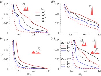
Next, we attempt to bring out the effect of different cavity regions on flow behaviour by analysing profiles of vertical time-averaged temperature,  $\langle \theta \rangle _t$. In figure 12, mean temperature profiles at different valleys (
 $V1$,
 $V2$ and
 $V3$) near the bottom plate are shown with increasing
 ${\textit {Ra}}$. The region corresponding to valley
 $V3$ is most spacious, while valley
 $V2$ is highly confined. It can be observed that the mean temperatures for
 $V1$ and
 $V2$ at
 ${\textit {Ra}}=10^8$ are nearly unity for a layer of fluid close to the wall. Note that the fluid layer with nearly zero temperature gradient is thicker in
 $V2$ than
 $V1$. However, for
 $V3$, this layer is hardly visible as the fluid is least confined, hence heat is diffused effectively in the vertical direction. Due to the severe confinement of fluid near the valley region, such a layer is observed. In the absence of confinement, a linearly varying thin layer is observed where temperature drops sharply. With the increase in
 ${\textit {Ra}}$, the temperature gradient increases significantly, resulting in a very thin layer over which practically half of the net imposed temperature drop occurs.
(a–c) Vertical mean temperature  $(\langle \theta \rangle _t)$ profile passing through three different valley regions,
 $V1$,
 $V2$ and
 $V3$, respectively, near the bottom plate, with increasing
 ${\textit {Ra}}$; these panels follow the same legend. In (d),
 $\langle \theta \rangle _t$ profiles for the valley regions are compared for the two extreme
 ${\textit {Ra}}$ (
 $10^8$ and
 $10^{11}$).

Note that in the succeeding discussion, the layer with a steep temperature gradient is discussed for the valleys, while the layer with trivial temperature gradient is not taken into consideration. It can be observed that  $\langle \theta \rangle _t$ is steepest for
 $V3$, while for
 $V2$, it is flattest for any
 ${\textit {Ra}}$. At the highest
 ${\textit {Ra}}=10^{11}$,
 $\langle \theta \rangle _t$ profiles for
 $V1$ and
 $V3$ are nearly same, as shown in figure 12(d), while
 $V2$ still exhibits smaller temperature gradients. This implies that as
 $V1$ is effectively washed out at
 ${\textit {Ra}}=10^{11}$, the flow characteristics become similar to
 $V3$, which is least confined and ventilated effectively by bulk fluid even at lower
 ${\textit {Ra}}$. However, as
 $V2$ is severely confined, heat is diffused slowly in the vertical direction even at
 ${\textit {Ra}}=10^{11}$, with the cavity region just starting to get washed out, resulting in the flattest
 $\langle \theta \rangle _t$.
In the present work,  $\langle \theta \rangle _t$ profiles passing through three different valleys of the bottom plate illustrate the effect of roughness wavelength on the heat transfer. It has been observed that flow structures are dependent on both
 ${\textit {Ra}}$ and wavelength of the roughness elements (Zhu et al. Reference Zhu, Stevens, Verzicco and Lohse2017, Reference Zhu, Stevens, Shishkina, Verzicco and Lohse2019; Zhang et al. Reference Zhang, Sun, Bao and Zhou2017b; Toppaladoddi et al. Reference Toppaladoddi, Succi and Wettlaufer2017). When elements are well spaced, and thermal forcing is strong enough to effect mixing in the cavities, a steeper
 $\langle \theta \rangle _t$ similar to the one in smooth surfaces is observed early. But for closely packed cavities, effective mixing of fluid is achieved at a much higher
 ${\textit {Ra}}$, hence steeper
 $\langle \theta \rangle _t$ profiles are achieved late. Highly confined cavity regions do not assist in enhancing heat transfer at low to moderate
 ${\textit {Ra}}$ owing to the lack of mobility of the fluid inside them. However, in the higher
 ${\textit {Ra}}$ range, as flow structures become finer, mobility is increased, hence these regions start to augment heat transfer. The same observation can be made from
 $\langle \theta \rangle _t$ profiles for
 $V2$. As the profiles, even at the highest
 ${\textit {Ra}}=10^{11}$, are still making the transition to a steeper smooth-surface like profiles, flow behaviour in these regions is still influenced by the rough surfaces. It is also known that when cavities are only partly washed by the bulk flow, enhanced heat transport scaling is achieved (Zhu et al. Reference Zhu, Stevens, Verzicco and Lohse2017). This explains why closely packed regions yield favourable results in the higher
 ${\textit {Ra}}$. The cavities that are dormant (stagnant fluid) at the lower
 ${\textit {Ra}}$ range start to get washed away by the bulk fluid in the higher
 ${\textit {Ra}}$ range. This implies that at the higher
 ${\textit {Ra}}$, roughness elements of smaller amplitude (small tips) or smaller wavelength (highly confined regions) are useful in retarding the arrival of the classical
 $1/3$ scaling. Note that it is expected that for a very high thermal forcing,
 ${\textit {Ra}}\gg 10^{11}$, the effect of the regions with smaller wavelength or severe confinement would also cease to exist, where
 $\langle \theta \rangle _t$ profiles for
 $V1$,
 $V2$ and
 $V3$ will become identical. Thus inclusion of very small wavelength elements acts as a remedy to cast away the classical scaling and thus extend the range of the augmented heat transfer scaling.
In thermal convection, the role of TBL ( $\lambda _\theta$) is pivotal. The transition of TBL attached to the isothermal plate to a turbulent state is still believed to have links with the so-called
 $1/2$ scaling regime. For the smooth plates, BL-dominated flow at low
 ${\textit {Ra}}$ makes a transition to bulk-dominated flow (Grossmann & Lohse Reference Grossmann and Lohse2000; Ahlers et al. Reference Ahlers, Grossmann and Lohse2009) at high
 ${\textit {Ra}}$, rendering the
 $1/2$ scaling regime. This idea has been modified recently. With the addition of roughness, bulk-dominated flow at lower
 ${\textit {Ra}}$ was reported (Zhu et al. Reference Zhu, Stevens, Verzicco and Lohse2017) to change to BL-based at high
 ${\textit {Ra}}$, reviving the classical
 $1/3$ scaling. This also implies that the roles of BL and bulk are reversed. A thin covering of TBL in the higher
 ${\textit {Ra}}$ range was reasoned to explain the fallback to
 $1/3$ scaling (Zhu et al. Reference Zhu, Stevens, Verzicco and Lohse2017) after a stint in
 $1/2$ scaling (Toppaladoddi et al. Reference Toppaladoddi, Succi and Wettlaufer2017). In the current work,
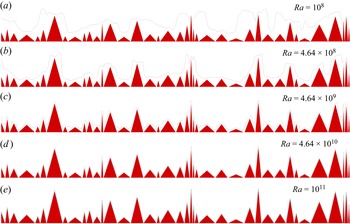
 $\lambda _\theta$ is calculated by taking the edge of the TBL at the position where temperature fluctuations are maximum (Tilgner, Belmonte & Libchaber Reference Tilgner, Belmonte and Libchaber1993), as shown by a schematic in figure 13. The computed BL profile along the
 $x$ direction is shown in figure 14, where roughness elements are also placed for better visibility of
 $\lambda _\theta$. At the lowest
 ${\textit {Ra}}=10^8$, taller roughness elements protrude into the TBL and thus are the major benefactor in enhancing heat transfer. With an increase in
 ${\textit {Ra}}$,
 $\lambda _\theta$ becomes thinner, and smaller roughness elements start to protrude into the TBL. The smaller elements play an important role in sustaining the plume emission at higher
 ${\textit {Ra}}$. At the highest
 ${\textit {Ra}}=10^{11}$, a nearly thin uniform TBL, except at the valleys, is formed along the rough surface. Note that for the valley regions, where the fluid is least mobile, a higher
 $\lambda _\theta$ is obtained. It is interesting to note that more the confinement, the thicker
 $\lambda _\theta$ is. Previously, Zhu et al. (Reference Zhu, Stevens, Shishkina, Verzicco and Lohse2019) predicted that the formation of a thin uniform TBL would lead to the classical
 $1/3$ scaling. Remarkably, in spite of a thin covering of the TBL with increasing
 ${\textit {Ra}}$, the
 ${\textit {Nu}}({\textit {Ra}})$ scaling does not saturate to the classical
 $1/3$ law at a very high
 ${\textit {Ra}}$ when random roughness is used. This again indicates the complex role of multi-scale roughness in turbulent convection.
Schematic showing a geometrical construction of TBL thickness ( $\lambda _\theta$). Note that profiles of temperature fluctuation start on the surface of a roughness element, and
 $\lambda _\theta$ is measured accordingly.

Variation of TBL thickness ( $\lambda _\theta$) over the bottom rough surface with increasing
 ${\textit {Ra}}$, where
 $\lambda _\theta$ is shown by black solid lines. At the lowest
 ${\textit {Ra}}=10^8$, only taller roughness elements protrude into the TBL, but with the increase in
 ${\textit {Ra}}$, smaller elements start to protrude. At the highest
 ${\textit {Ra}}=10^{11}$, a thin uniform TBL, except at the valleys, is seen to cover the rough surface.

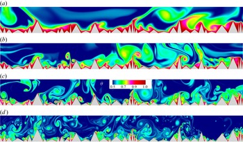
To visualize local flow structures, the instantaneous temperature field in the near-wall region of the bottom hot plate is shown in figure 15. It is evident that at  ${\textit {Ra}}=10^8$, the roughness elements are covered by a thick layer of hot fluid, implying that flow is stagnant near the surface. Also, plumes, which are emitted from the taller elements, are of larger size. With the increase in
 ${\textit {Ra}}$, the layer of hot fluid covering the surface starts to become thinner, and the fluid inside the cavities starts to move out of it. Also, plumes become finer, with a surge in nucleation sites owing to the increased contributions from the smaller elements. At the highest
 ${\textit {Ra}}=10^{11}$, plumes are extremely fine, and almost all the elements are participating actively in plume emission. Further, penetration of the bulk fluid inside the cavities is maximized, due to which highly confined regions also start to become accessible to the bulk. Though flow structures become finer, enhancement in heat transfer occurs with the increase in plume emission sites at the highest
 ${\textit {Ra}}$, which contributes primarily in sustaining the enhanced heat transport regime.
Instantaneous temperature field for near-wall region corresponding to the hot bottom plate for (a)  ${\textit {Ra}}=10^8$, (b)
 ${\textit {Ra}}=10^9$, (c)
 ${\textit {Ra}}=10^{10}$, and (d)
 ${\textit {Ra}}=10^{11}$. At the lowest
 ${\textit {Ra}}$, plumes are of larger size with a few emitting spots; however, as
 ${\textit {Ra}}$ increases, there is a surge in plume-emitting spots with visibly finer flow structures. Also, the ability of the bulk fluid to invade highly confined cavity or tip regions of the smaller roughness elements is enhanced significantly at a higher
 ${\textit {Ra}}$, which augments heat transfer.

Enhancement in heat transfer depends on the amplitude (Zhang et al. Reference Zhang, Sun, Bao and Zhou2017b) and wavelength (Toppaladoddi et al. Reference Toppaladoddi, Succi and Wettlaufer2017) of roughness elements. When the amplitude is of the order of the TBL thickness, enhancement in heat transfer is perceived, which is observed in the present study from instantaneous temperature contours, p.d.f.s and time series of temperature and vertical velocity. This explains why smaller roughness elements play an important role in sustaining heat transfer at the higher  ${\textit {Ra}}$ range. Previously, Toppaladoddi et al. (Reference Toppaladoddi, Succi and Wettlaufer2017) explored the effect of the wavelength through sinusoidal roughness on the scaling exponent, where it was observed that too large or small wavelength yields the scaling exponent close to
 $1/3$. However, the range (
 $4\times 10^6 \leq {\textit {Ra}} \leq 3\times 10^9$) explored by them was not high enough to realize the propitious results of the rough surface with a small wavelength. Later, Zhang et al. (Reference Zhang, Sun, Bao and Zhou2017b), in their study with mono-scale triangular roughness, established the efficacy of the rough surfaces with smaller amplitude by highlighting that the critical height (
 $h_c$) of the rough surfaces signifying enhanced heat transfer in comparison to smooth surfaces decreases with
 ${\textit {Ra}}$ as
 $h_c \sim {\textit {Ra}}^{-0.6}$. Zhu et al. (Reference Zhu, Stevens, Verzicco and Lohse2017, Reference Zhu, Stevens, Shishkina, Verzicco and Lohse2019) took into account the effect of both the parameters together by introducing the roughness aspect ratio, defined as the ratio of the amplitude to the wavelength of roughness elements. Also, they ran different tests to ascertain the optimum roughness aspect ratio yielding the maximum scaling exponent, which was reported as unity. This implies that rough surfaces with smaller amplitude and wavelength are highly effective at a higher
 ${\textit {Ra}}$. The results obtained for our multi-scale random roughness configuration are in agreement with the above observations. Hence the inclusion of random roughness has proved to be highly beneficial in sustaining enhanced heat transfer even at the higher
 ${\textit {Ra}}$ range owing to the creation of different local regions that are activated at different thermal forcings.
The attempt to incorporate multi-scale roughness paid off outstandingly, such that different relative locations contributed differently in the plume-emission process to avoid saturation of the increased heat transfer scaling. Taller roughness elements exhibited large temperature fluctuations at lower  ${\textit {Ra}}$, while throat regions were dormant initially. However, with increasing thermal forcing, contributions from the throat regions further propelled the separation of the plumes from the tip regions. Though a thin TBL is formed at a higher
 ${\textit {Ra}}$, increased contributions from the small-scale elements and the activation of the highly confined regions continued to amplify the overall perturbations in the near-wall regions, leading to enhanced heat transport. The TBL envelopes roughness elements hierarchically, starting from the tallest to the shortest with increasing thermal forcing. However, the complex texture of the roughness acts as a deterrent to a uniform covering of the TBL over it. Thus the earlier reported state, where the rough surfaces were practically reduced to smooth only with extended wetted surface area, is deferred.
3.4. Bulk dynamics
We now turn our attention to the flow dynamics away from the rough surfaces. With plumes emitting from the rough surfaces and moving into the bulk region, the fluctuations are brought about by them. In line with the results of a number of studies (Du & Tong Reference Du and Tong2001; Stringano et al. Reference Stringano, Pascazio and Verzicco2006), the increased temperature fluctuations in comparison to the smooth case are observed in the present study. In figure 16, horizontally averaged r.m.s. of temperature ( $\sigma _\theta$) and vertical fluctuations (
 $\sigma _v$) at mid-height of the cell (
 $y = 0.5$) are shown along with the smooth case counterparts (Chand et al. Reference Chand, Sharma, Sharma and De2019) as a function of
 ${\textit {Ra}}$. It is clearly evident that
 $\sigma _\theta$ is magnified in the presence of the rough surfaces, while
 $\sigma _v$ is comparable to that observed in the smooth case. Also, the distinct nature of
 $v^\prime$ and
 $\theta ^\prime$ is unveiled, with
 $\sigma _\theta$ decreasing monotonically with increasing
 ${\textit {Ra}}$, while large-amplitude
 $v^\prime$ are marked by the peak in
 $\sigma _v$ at higher
 ${\textit {Ra}}$. Surprisingly,
 $\sigma _v$, as opposed to
 $\sigma _\theta$, increases monotonically before reaching a peak near
 ${\textit {Ra}}=2.15\times 10^{10}$. The difference in the trend for
 $\sigma _v$ and
 $\sigma _\theta$ can be attributed to the interaction of the high-intensity rolls with the background, which causes large-amplitude vertical velocity fluctuations at a higher Ra while temperature oscillations are damped out due to vigorous mixing of the fluid.
Variation of horizontally averaged r.m.s. of fluctuations of (a) temperature ( $\sigma _\theta$), and (b) vertical velocity (
 $\sigma _v$), at mid-height of the cell (
 $y=0.5$) as a function of
 ${\textit {Ra}}$. For comparison, the data corresponding to the smooth surface (Chand et al. Reference Chand, Sharma, Sharma and De2019) are also shown.

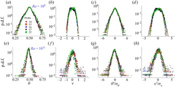
The scattered and skewed distribution of  $\theta ^{\prime }$ is not expected in the bulk as polarized fluctuations near the wall give way to oscillations about the bulk mean temperature. In figure 17, we observe that the p.d.f.s corresponding to different probes in bulk overlap with each other at a particular
 ${\textit {Ra}}$, signifying that the overall flow behaviour is nearly the same at different horizontal locations in the bulk. At the lowest
 ${\textit {Ra}}=10^8$, they are wider about the mean (
 $\theta =0.5$), but with the increase in
 ${\textit {Ra}}$, they become narrower, implying that the probability of occurrence of the structures with large temperature gradient is diminished, and at the same time, bulk fluid approaches a uniform temperature (
 $\theta =0.5$). Non-obeyance of the Gaussian distribution (Castaing et al. Reference Castaing, Gunaratne, Heslot, Kadanoff, Libchaber, Thomae, Wu, Zaleski and Zanetti1988; Kandanoff Reference Kandanoff2001; Wang, He & Tong Reference Wang, He and Tong2019) near the tails of the p.d.f.s of
 $v^\prime$ and
 $\theta ^\prime$ at
 ${\textit {Ra}}=10^{11}$ reflects the intermittent appearance of the large-amplitude events in the bulk, which are enhanced significantly with the introduction of the random rough surface.
P.d.f.s of (a,e) temperature ( $\theta$), and (b, f) vertical velocity (
 $v$); and normalized fluctuations of (c,g) temperature (
 $\theta ^\prime /\sigma _\theta$), and (d,h) vertical velocity (
 $v^\prime /\sigma _v$), for probes in bulk. Note that (a–d) corresponds to the lowest
 ${\textit {Ra}}=10^8$, while (e–h) are for the highest
 ${\textit {Ra}}=10^{11}$. The solid lines in (c,d,g,h) represent the Gaussian function. See figure 8(b) for the locations of the probes.

Power spectra of the vertical velocity and temperature in the bulk can be analysed to evaluate the energy cascade and the associated small-scale dynamics. The slope in the inertial subrange (Pope Reference Pope2000; Lohse & Xia Reference Lohse and Xia2010) is of particular interest to the research community. The classical view of the scaling in the inertial subrange is that for a homogeneous and isotropic flow, temperature and velocity fluctuations follow Kolmogorov's K41 scaling (Kolmogorov Reference Kolmogorov1941; Obukhov Reference Obukhov1949; Corrsin Reference Corrsin1951). Obeyance of the K41 scaling implies that temperature is a passive scalar. However, for an anisotropic flow, the BO59 scaling proposed by Bolgiano (Reference Bolgiano1959) and Obukhov (Reference Obukhov1959) is expected for the fluctuations where temperature exhibits characteristics of an active scalar. According to the K41 scaling, the slope in the inertial subrange for both velocity and temperature spectra is  $-5/3$, while for the BO59 scaling, the slope becomes
 $-7/5$ for temperature as opposed to
 $-11/5$ for velocity.
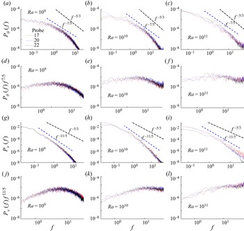
In figure 18, power spectra of temperature and vertical velocity are shown for three probes in the bulk, one above a throat region, and the remaining two directly above the tips, at three different  ${\textit {Ra}}$ values,
 $10^9$,
 $10^{10}$ and
 $10^{11}$. It can be observed that both temperature and velocity follow the BO59 scaling as the slopes in the inertial subrange are close to
 $-7/5$ and
 $-11/5$ for temperature and velocity, respectively. The same observation is also evident from compensated plots of temperature and vertical velocity spectra in figures 18(d–f,j–l), respectively. It is evident that with the increase in
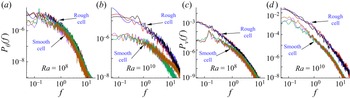
 ${\textit {Ra}}$, the inertial range obeying the BO59 scaling also widens. Previously, Stringano et al. (Reference Stringano, Pascazio and Verzicco2006), in their study in a cylindrical cell with grooved surfaces, reported BO59 scaling for temperature and K41 scaling for vertical velocity in the bulk of the flow. However, in the present study, we observe that temperature behaves as a pure active scalar. Also, the spectra for the present work are compared with those observed for the smooth surface case (Chand et al. Reference Chand, Sharma, Sharma and De2019) at
 ${\textit {Ra}}=10^8$ and
 $10^{10}$ at mid-height of the cell, as shown in figure 19. At
 ${\textit {Ra}}=10^8$, both temperature and velocity spectra are comparable with those observed for the smooth case, which signifies nearly the same level of fluctuations. However, at
 ${\textit {Ra}}=10^{10}$, both spectra show increased energy at all scales of the flow in comparison to the smooth surface, highlighting the effectiveness of the roughness at higher
 ${\textit {Ra}}$. Thus the presence of the random roughness is perceived in the bulk through increased temperature fluctuations in comparison to the smooth cell. Though flow homogeneity in the temperature sense increases with
 ${\textit {Ra}}$, its fluctuations continue to be higher than the smooth cell due to the increased presence of plumes emitted from the rough surfaces in the bulk.
Power spectra of (a–c) temperature, and (g–i) vertical velocity for the bulk at three different  ${\textit {Ra}}$ values,
 $10^9$,
 $10^{10}$ and
 $10^{11}$. The corresponding compensated plots of (d–f) temperature, and ( j–l) vertical velocity spectra, are also shown. Note that the dashed lines represent the scaling of Bolgiano and Obukhov (denoted BO59) ((Bolgiano Reference Bolgiano1959; Obukhov Reference Obukhov1959), with slopes
 $-7/5$ and
 $-11/5$ for temperature and vertical velocity spectra, respectively. Further, the dash-dot lines serve as a reference for Kolmogorov's scaling (denoted K41). See figure 8(b) for the locations of the probes.

Power spectra of (a,b) temperature, and (c,d) vertical velocity, for the rough cell are compared with those observed for the smooth surface case (Chand et al. Reference Chand, Sharma, Sharma and De2019) at  ${\textit {Ra}}=10^8$ and
 $10^{10}$ for probes considered at mid-height of the cells at three different horizontal locations (
 $x=0.5,1,1.5$).

3.5. Small-scale statistics
In turbulent RBC, the imposed temperature difference between the plates induces a buoyancy force, which sets the fluid in motion. According to Richardson (Reference Richardson1922), the energy from the large-scale eddies is passed on to the smaller eddies until it is dissipated at small scales, where molecular diffusivity becomes predominant. The process of transfer of energy in the inertial subrange holds the answers to various scaling laws followed by velocity and temperature fluctuations (Camussi & Verzicco Reference Camussi and Verzicco2004; Kunnen et al. Reference Kunnen, Clercx, Geurts, Bokhoven, Akkermans and Verzicco2008; Lohse & Xia Reference Lohse and Xia2010; Kaczorowski & Xia Reference Kaczorowski and Xia2013). In view of homogeneous and isotropic flow (Kolmogorov Reference Kolmogorov1941; Corrsin Reference Corrsin1951; Obukhov Reference Obukhov1949), temperature is treated as a passive scalar, and the effect of buoyancy force at small scales is neglected. The scalings for the fluctuations can be found by invoking energy balance between the energy transfer and dissipation:
 \begin{equation} \left. \begin{aligned} & \epsilon_u \sim\frac{(\delta u)^3}{l} , \quad \epsilon_T \sim \frac{\delta u\,(\delta T)^2}{l},\\ & \implies \delta u \sim \epsilon_u^{1/3} l^{1/3}, \quad \delta T \sim \epsilon_u^{{-}1/6} \epsilon_T^{1/2} l^{1/3}, \end{aligned} \right\} \end{equation}
where  $\delta u$ and
 $\delta T$ are the differences in velocity (
 $u$) and temperature (
 $T$) between two points separated by a distance
 $l$, respectively,
 $\epsilon _u$ is the viscous dissipation, and
 $\epsilon _T$ is the thermal dissipation. Another viewpoint for scaling in the inertial subrange was proposed by Bolgiano (Reference Bolgiano1959) and Obukhov (Reference Obukhov1959), where above a characteristic length scale, defined as the Bolgiano length scale (
 $L_B$), buoyancy forces become important. Now the scaling for the velocity fluctuations are found by invoking energy balance between the down-scale energy transfer and buoyancy production, while for temperature fluctuations, the energy transfer is again balanced by the thermal dissipation:
 \begin{equation} \left. \begin{aligned} & \frac{(\delta u)^3}{l} \sim \beta g\,\delta u\,\delta T, \quad\epsilon_T \sim \frac{\delta u\, (\delta T)^2}{l},\\ & \implies \delta u \sim (\beta g)^{2/5}\epsilon_T^{1/5} l^{3/5}, \quad \delta T \sim (\beta g)^{{-}1/5} \epsilon_T^{2/5} l^{1/5}. \end{aligned} \right\} \end{equation}
Ideally, for scales  $\eta \ll l\ll L_B$, the Kolmogorov K41 scaling should be realized, while for
 $L_B \ll l \ll H$, the Bolgiano and Obukhov BO59 scaling is expected (Lohse & Xia Reference Lohse and Xia2010), where
 $\eta$ and
 $H$ are the Kolmogorov length scale and height of the cell, respectively. The cross-over between these two scalings yields the Bolgiano length scale, which implies
 \begin{equation} \left. \begin{aligned} & \quad \epsilon_u^{1/3} L_B^{1/3} = (\beta g)^{2/5} \epsilon_T^{1/5} L_B^{3/5}\quad\text{or}\quad \epsilon_u^{{-}1/6} \epsilon_T^{1/2} L_B^{1/3}= (\beta g)^{{-}1/5} \epsilon_T^{2/5} L_B^{1/5},\\ \implies & \quad L_B = (\beta g)^{{-}3/2} \epsilon_u^{5/4} \epsilon_T^{{-}3/4}. \end{aligned} \right\} \end{equation}
In the non-dimensionalized form,  $L_B$ is found as
 \begin{equation} L_B= \epsilon_u ^{5/4} \epsilon_\theta^{{-}3/4}, \end{equation}
where  $\epsilon _u, \epsilon _\theta$ are computed from the non-dimensional field. In turbulent RBC, simultaneous existence of both scalings is usually not observed (Lohse & Xia Reference Lohse and Xia2010). Also, whether the BO59 scaling, which was first proposed for stably stratified flows, exists for RBC is still unresolved. Kunnen et al. (Reference Kunnen, Clercx, Geurts, Bokhoven, Akkermans and Verzicco2008) and Kunnen & Clercx (Reference Kunnen and Clercx2014) addressed the relation between the mean Bolgiano length scale (using global values of the dissipation rates) and the BO59 scaling. They proposed that
 $L_B$ should be considered locally, while looking for the BO59 scaling as the order of magnitude of the dissipation rates is substantially high in the near-wall regions in comparison to the bulk. Local
 $L_B$ attains small values close to the isothermal walls, while it has large values in the bulk region. Further, it increases with an increase in
 ${\textit {Ra}}$ in the bulk region, while mean/global
 $L_B$ decreases with
 ${\textit {Ra}}$. This highlights the subtleties to consider while deducing the relationship between the order of
 $L_B$ and the possible scaling for the fluctuations.
To verify the existence of the Bolgiano scaling in the bulk region, as observed from figure 18, we explore different measures of  $L_B$. In figure 20(a), vertical variation of the horizontally time-averaged Bolgiano length
 $\langle L_B \rangle _{A,t}=\langle \epsilon _u\rangle ^{5/4} _{A,t} \langle \epsilon _\theta \rangle ^{-3/4} _{A,t}$ as a function of
 ${\textit {Ra}}$ is shown. It can be observed that in general,
 $\langle L_B \rangle _{A,t}$ increases with
 ${\textit {Ra}}$ in the bulk region. However, the maximum value is of the order of
 $H/10$, which is far separated from
 $H$. This partly supports the existence of the Bolgiano scaling observed earlier in the
 $v$ and
 $\theta$ spectra. Further, for comparison,
 $\langle L_B \rangle _{A,t}$ for the smooth surface case (Chand et al. Reference Chand, Sharma, Sharma and De2019) is shown in figure 20(b). The trend and the order of
 $L_B$ are comparable to what is observed in the present work away from the walls. Clearly, owing to a high
 $\epsilon _\theta$ near the walls, the local measure of
 $L_B$ drops there significantly. However, in the bulk, it shows a global maximum as the flow is nearly homogeneous. We observe a consistent trend in both the rough and smooth geometries, with
 $L_B$ increasing marginally with
 ${\textit {Ra}}$.
Variation of horizontally time-averaged Bolgiano length scale  $\langle L_B\rangle _{A,t}={\langle \epsilon _u \rangle }_{A,t} ^{5/4} {\langle \epsilon _\theta \rangle }_{A,t} ^{-3/4}$ as a function of vertical distance
 $y$ in (a) the present roughness set-up, and (b) the smooth surface case (Chand et al. Reference Chand, Sharma, Sharma and De2019), for different
 ${\textit {Ra}}$. (c) Global Bolgiano length scales
 $L_B^g$ and
 $L_B^{A}$ as functions of
 ${\textit {Ra}}$. Also,
 $L_B^g$ for smooth plates (Chand et al. Reference Chand, Sharma, Sharma and De2019) is shown. Note that
 ${L_B^g=\langle \epsilon _u \rangle }_{V,t} ^{5/4} {\langle \epsilon _\theta \rangle }_{V,t} ^{-3/4}$, while
 $L_B^{A}$ is obtained by taking the vertical average of
 $\langle L_B\rangle _{A,t}$. The vertical extent of the shaded regions in (a) represents the maximum height of the roughness elements.

Theoretically, global estimate of  $L_B$ can be approximated by using global estimates of thermal and kinetic dissipation rates (Shraiman & Siggia Reference Shraiman and Siggia1990) in (3.8):
 \begin{equation} \left. \begin{aligned} \langle \epsilon_u \rangle_{V,t} & = \frac{{\textit{Nu}}-1}{\sqrt{{\textit{Ra}}\,{\textit{Pr}}}}, \quad \langle \epsilon_\theta \rangle_{V,t}= \frac{{\textit{Nu}}}{\sqrt{{\textit{Ra}}\,{\textit{Pr}}}} ,\\ \implies L_B^g & = \langle\epsilon_u\rangle^{5/4}_{V,t} \langle\epsilon_\theta\rangle^{{-}3/4}_{V,t}=\left(\frac{{\textit{Nu}}-1}{\sqrt{{\textit{Ra}}\,{\textit{Pr}}}}\right)^{5/4} \left(\frac{{\textit{Nu}}}{\sqrt{{\textit{Ra}}\,{\textit{Pr}}}}\right)^{{-}3/4},\\ \implies L_B^g & \approx {\textit{Nu}}^{1/2}/({\textit{Ra}}\,{\textit{Pr}})^{1/4} \quad (\text{for}\ {\textit{Nu}} \gg 1). \end{aligned} \right\} \end{equation}
A second global measure of  $L_B$ can also be obtained by integrating
 $\langle L_B\rangle _{A,t}$ vertically:
 \begin{equation} L_B^A=\int_0^H \langle L_B\rangle_{A,t} (y)\, {{\rm d} y}. \end{equation}
While  $L_B^g$ includes the spatial inhomogeneity of
 $\epsilon _{\theta }$ arising from bulk–plume interaction,
 $L_B^A$ strikes a compromise between the gap in
 $\langle L_B\rangle _{A,t}$ in the bulk and near-wall region. We show their variation in figure 20(c) as a function of
 ${\textit {Ra}}$. With the
 ${\textit {Nu}} \sim {\textit {Ra}}^{1/2}$ scaling, the above scaling predicts a
 ${\textit {Ra}}$-invariant
 $L_B^g$. Both the global measures nearly conform to this argument. Further, we note that both
 $L_B^g$ and
 $L_B^{A}$ have smaller magnitudes than
 $\langle L_B \rangle _{A,t}$ as they are not as sensitive to
 $\epsilon _{\theta }$ as the local measure is. Also,
 $L_B^g$ for the smooth surface (Chand et al. Reference Chand, Sharma, Sharma and De2019) is appended in figure 20(c), where it is seen to drop with increasing
 ${\textit {Ra}}$. With the classical
 ${\textit {Nu}} \sim {\textit {Ra}}^{1/3}$ scaling inserted in (3.9), one obtains
 $L_B^g \sim {\textit {Ra}}^{-1/12}$. The power-law fitting of
 ${\textit {Ra}}^{-1/12}$ follows closely the smooth surface data. In the current work,
 $L_B$ is found to be in the admissible limits (not greater than
 $H$) for the realization of the Bolgiano scaling for the explored
 ${\textit {Ra}}$ range, which is in agreement with the spectra obtained for temperature and velocity fluctuations in the bulk. In addition, global Bolgiano length appears to support the classical
 $1/3$ scaling for the smooth surface data, while the much elusive
 $1/2$ scaling shows encouraging signs of consistency with the estimate
 $L_B^g \approx {\textit {Nu}}^{1/2}/({\textit {Ra}}\,{\textit {Pr}})^{1/4}$. Note that in spite of substantial evidence in favour of existence of the BO59 scaling from different estimates of
 $L_B$, the result can be claimed incontestable only when complemented by the results of the spatial structure functions of temperature and velocity. Also, the two-dimensionality of the problem introduces further complications due to the effect of inverse energy cascade (Boffetta & Ecke Reference Boffetta and Ecke2012). Thus in view of the above considerations, caution must be exercised while invoking the BO59 scaling.
3.6. Decomposition into orthogonal modes
In order to identify the dominant organized mode of heat transfer mechanism and the much elusive coherent structure, we have decomposed the flow field into a number of orthogonal modes. The basic principle behind proper orthogonal decomposition (POD) (Berkooz, Holmes & Lumley Reference Berkooz, Holmes and Lumley1993) is to seek an optimal basis of orthogonal spatial modes or eigenfunctions for a vector field  $\boldsymbol {U}(\boldsymbol {r},t)$ based on its energy content
 $\int \langle \boldsymbol {U}(\boldsymbol {r},t)^2 \rangle _t \, \textrm {d}\boldsymbol {r}$. The vector field
 $\boldsymbol {U}(\boldsymbol {r},t)$ can be written as a superposition of the spatial modes
 $\boldsymbol {\phi }_n(\boldsymbol {r})$ scaled by their temporal amplitudes
 $a_n(t)$ in the following manner:
 \begin{equation} \boldsymbol{U}(\boldsymbol{r},t) = \sum_{n=1}^{\infty} a_n(t)\,\boldsymbol{\phi}_n(\boldsymbol{r}). \end{equation}
Note that the POD modes are arranged in decreasing order of their energy indicated by the eigenvalues of an algebraic problem discussed below. To represent the vector field  $\boldsymbol {U}(\boldsymbol {r},t)$ in a low-dimensional subspace, the decomposition can be restricted to the first few modes, encapsulating a large portion of the energy of
 $\boldsymbol {U}(\boldsymbol {r},t)$. While applying POD to the natural convection problem, one needs to decide whether to treat velocity and temperature jointly or independently (Lumley & Poje Reference Lumley and Poje1997; Podvin & Sergent Reference Podvin and Sergent2017; Soucasse et al. Reference Soucasse, Podvin, Riviére and Soufiani2019). The former treatment takes into account the coupling of temperature and velocity with the introduction of a scaling factor
 $\gamma$. In the present work, the vector field considered is
 $\boldsymbol {U}(\boldsymbol {r},t)=[u,v,\gamma \theta ]$, where
 $\gamma$ is calculated as
 \begin{equation} \gamma= \left(\left\langle \frac{{\int}[u^2(\boldsymbol{r},t)+v^2(\boldsymbol{r},t)]\,{\rm d}\boldsymbol{r}}{{\int}\theta^2(\boldsymbol{r},t)\,{\rm d}\boldsymbol{r}} \right\rangle_t\right)^{1/2}, \end{equation}
which essentially allows the energy of both temperature and velocity field to be the same. The value of  $\gamma$ is obtained as 1.303.
The most energetic modes of POD have been looked up consistently to observe the large-scale structures and determine their role in the heat transfer process. A better understanding of these structures holds the key to achieve a greater heat transfer rate. Verdoold, Tummers & Hanjalić (Reference Verdoold, Tummers and Hanjalić2009) observed that the primary mode consists of a single roll covering the entire width of the cell at  ${\textit {Ra}} = 6\times 10^8$, while fluctuating modes revealed two types of flow patterns. In the first type, higher-order modes had an increased number of rolls. However, for the second type, second- and third-order fluctuating modes depicted diagonal flow patterns. Both types of fluctuating modes appeared randomly in repeated experiments for the same thermal forcing. Podvin & Sergent (Reference Podvin and Sergent2012), using the LES data, predicted that the first two most energetic modes, major benefactors in the vertical heat transfer, consist of rolls aligned in the transverse dimension, while for the subsequent modes they align in the longitudinal direction. Later, Podvin & Sergent (Reference Podvin and Sergent2015, Reference Podvin and Sergent2017) used the POD modes to investigate the flow structures to seek reasons for the observed flow reversals and cessations. 2-D geometry was preferred as it locks the LSC, allowing the disentanglement of the different mechanisms involved in flow reversals. The first three POD modes revealed the dominant structures as LSC consisting of a single-roll, symmetry breaking two rolls, and a quadrupolar flow. They observed that flow reversals are associated with the instability of the transient double-roll symmetry breaking mode. So far, POD has been used mainly as a tool to study the features of LSC and its reversals, notably in the low
 ${\textit {Ra}}$ range.
To extract the POD modes, we have implemented the method of snapshots (Sirovich Reference Sirovich1987), which essentially allows the modes to be written as a linear combination of  $N$ instantaneous snapshots of the vector field
 $\boldsymbol {U}(\boldsymbol {r},t)$ taken at different time instances
 $t_i$:
 \begin{equation} \boldsymbol{\phi}_n(\boldsymbol{r})=\sum_{i=1}^N \boldsymbol{U}(\boldsymbol{r},t_i)\,\varphi_n^i. \end{equation}
The vectors  $\boldsymbol {\varphi }_n$ are found from the algebraic eigenvalue problem
 \begin{equation} \boldsymbol{C\varphi}_n=\lambda_n \boldsymbol{\varphi}_n, \end{equation}
where  $\boldsymbol {C}$ is the temporal correlation matrix of the snapshots, calculated as
 \begin{equation} C_{ij}=\frac{1}{N}\displaystyle\int_V\left( \boldsymbol{u}(\boldsymbol{r},t_i) \boldsymbol{\cdot} \boldsymbol{u}(\boldsymbol{r},t_j)+\gamma^2\,\theta(\boldsymbol{r},t_i)\,\theta(\boldsymbol{r},t_j) \right) {\rm d}\boldsymbol{r}. \end{equation}
For the lowest  ${\textit {Ra}}=10^8$, a total of 400 snapshots are extracted at an interval of 2.5 time units, while for the highest
 ${\textit {Ra}}=10^{11}$ case, nearly 100 discrete temporal frames recorded at an interval of 0.5 time units are used to construct the eigenmodes. Such a choice is driven by collection of adequate number of time frames to include all possible random events without significant overlap.
In figure 21, the POD eigenspectrum normalized by  $\sum _N \lambda _i$ is shown along with the cumulative spectrum for
 ${\textit {Ra}} =10^8$,
 $10^9$,
 $10^{10}$ and
 $10^{11}$. Note that owing to such normalization, the cumulative sum
 $\sum _i \lambda _i$ approaches unity as one moves towards the right end of the spectrum. It can be observed that the first mode captures most of the energy. For
 ${\textit {Ra}}=10^8$ the energy captured by the first mode is 77 %, while for
 ${\textit {Ra}} =10^{11}$ it is 62 %. The cumulative spectrum indicates that with increase in
 ${\textit {Ra}}$, energy content in higher-order modes is non-trivial. This occurs owing to the enhanced inter-scale energy transfer and complexity of flow modes at higher thermal forcing.
Normalized POD eigenspectrum (filled symbols), where  $\varSigma _N \lambda _j=1$, is shown along with the associated cumulative spectrum (unfilled symbols) for
 ${\textit {Ra}} =10^8$,
 $10^9$,
 $10^{10}$ and
 $10^{11}$. The difference in energy content between the first- and higher-order modes indicates better mixing and inter-scale energy transfer at higher
 ${\textit {Ra}}$.

The temperature field superimposed with velocity vectors is shown for the first and second modes for  ${\textit {Ra}}=10^8$,
 $10^{10}$ and
 $10^{11}$ in figure 22. The first mode is seen to represent weakly the mean flow field, where a layer with very hot (bottom plate) or cold (top plate) fluid covering the rough surfaces is revealed. Also, the layer enclosing large temperature gradients diminishes with increased thermal forcing, though not uniformly, due to the intricate texture of the rough surfaces. It also signifies thinning of the TBL. In the bulk, the mean temperature field is nearly homogeneous, with higher
 $\theta$ at
 ${\textit {Ra}} =10^8$ in comparison to
 ${\textit {Ra}}=10^{10}$ and
 $10^{11}$, where it approaches 0.5. The temperature field corresponding to the second mode is at first inhomogeneous, but at the highest
 ${\textit {Ra}}=10^{11}$, we observe increased homogeneity. In the dominant mode, nearly half of the total temperature drop is noticed near the isothermal walls, with a large homogeneous bulk region. The second mode is clearly underdeveloped, and its contribution in heat transport is rather insignificant. Interestingly, the covering of TBL on the rough surface is detected only in the dominant first mode, while the subsequent mode exhibits only trapped fluid scattered around the throats of the roughness.
First (a,c,e) and second (b,d, f) POD modes representing the temperature field with superimposed velocity vectors for  ${\textit {Ra}}=10^8$ (a,b),
 ${\textit {Ra}}=10^{10}$ (c,d), and
 ${\textit {Ra}}=10^{11}$ (e, f). The bulk region clearly assumes a better homogeneous state with near bulk-mean temperature in the first mode, while underdeveloped and unmixed hot (or cold) plumes constitute the second mode.

From the velocity vector field shown in figure 22, the dominant double-roll structure (DRS) at  ${\textit {Ra}}=10^8$, observed readily from the first mode, is seen to transform into multiple small-scale rolls at the higher
 ${\textit {Ra}}$. Increased turbulence with emergence of the small structures from numerous sites near the rough surfaces supports disintegration of the large-scale rolls leading to the formation of the local vortices. The second POD mode for both
 ${\textit {Ra}}=10^8$ and
 ${\textit {Ra}}=10^{10}$ corresponds to the double-roll state, while at
 ${\textit {Ra}}=10^{11}$, multiple small-scale rolls are evident. The above observation hints that with increasing thermal forcing, organization of the flow with multiple small-scale rolls becomes the natural choice. While DRS at smaller
 ${\textit {Ra}}$ induces a stronger lateral motion, multiple small rolls at higher
 ${\textit {Ra}}$ promotes direct injection of plumes into the bulk, causing an increased
 $v\theta$ correlation responsible for enhanced heat flux. In figure 23, we show the normalized Nusselt number given by
 ${\textit {Nu}}=({\textit {Ra}}\, {\textit {Pr}})^{1/2}v\theta - \partial _y \theta$ computed from the first two modes for the selected
 ${\textit {Ra}}$. Note that the global maximum of
 ${\textit {Nu}}$ is used to normalize it. In agreement with our previous observation, at the lowest
 ${\textit {Ra}}$, dominant flow structures carrying a large amount of thermal energy are larger in size, while at higher
 ${\textit {Ra}}$, fine structures are responsible for the transport of heat. A greater vertical motion induced by multiple small-scale plumes improves the
 ${\textit {Nu}}$ distribution at higher
 ${\textit {Ra}}$, which is seen to be confined at smaller
 ${\textit {Ra}}$. Thus stable DRS as a principal carrier of heat does not favour an enhanced heat flux regime, while multiple small pockets of intense plumes distribute thermal energy efficiently and also create numerous nucleation sites for plumes. Breakdown of DRS into multiple rolls is triggered by the sharp peaks and uneven valleys near the isothermal surfaces.
Normalized Nusselt numbers  ${\textit {Nu}}_n$ calculated from the first (a,c,e) and second (b,d, f) modes are shown for
 ${\textit {Ra}}=10^8$ (a,b),
 ${\textit {Ra}}=10^{10}$ (c,d), and
 ${\textit {Ra}}=10^{11}$ (e, f). Note that the maximum value of
 ${\textit {Nu}}$ is used for its normalization. The dominant mode of heat transfer occurs with multiple unstable structures, while the secondary mode mainly shows the stable double-roll state.

4. Summary and conclusions
The present work explored the effect of random triangular roughness on the flow dynamics and heat transport properties in a 2-D rectangular cell. The inclusion of varied elements enriched the flow physics such that they and the associated regions assumed distinct roles to enable the sustenance of the enhanced heat transfer scaling throughout the explored three decades of  ${\textit {Ra}}$. At lower
 ${\textit {Ra}}$, only taller elements are active in enhancing plume emission from their tips, while at higher
 ${\textit {Ra}}$, substantial contributions from the smaller elements are received, which play a pivotal role in casting aside the saturation of the enhanced heat transport scaling. Plume regions are identified clearly by high convective heat flux and are observed to be the most potent coherent structures in enhancing the heat transfer at all thermal forcings. Increased plume-emission frequency in comparison to the smooth surface case is quantified from turbulent buoyancy production and dissipation, and volume fraction of plumes. Detailed analysis of the near-wall dynamics reveals the complex role of the roughness elements and the associated throat, cavity and tip regions. Throat regions are inaccessible to the bulk flow at lower
 ${\textit {Ra}}$. However, with increasing thermal forcing, penetration of the bulk fluid improves, which is also reflected through increased velocity fluctuations. Similarly, tip regions associated with smaller roughness elements get activated at higher
 ${\textit {Ra}}$, such that they start to protrude into the TBL and incite plume emissions that are recorded from temperature fluctuations.
Also, distinct flow dynamics in different throat regions are revealed through vertical profiles of mean temperature passing through the associated valleys. Evolution of the flatter linear profiles to the steeper ones, identical to that observed in a smooth cell for highly confined cavities from the lowest  ${\textit {Ra}}$ to higher
 ${\textit {Ra}}$, marks the washing away of the cavities. When profiles become identical to that of the smooth cell, the effect of the cavity regions in perturbing the nearby flow is largely diminished. Depending on whether throat regions are spacious or confined, the transition to enhanced local heat flux regime happens at different thermal forcings. This implies that the propitious effect of the roughness elements is not lost altogether. Activation of small-scale roughness elements and highly confined regions at higher
 ${\textit {Ra}}$ promotes the sustenance of the enhanced heat transfer scaling. Further, the effect of perturbations induced by the roughness elements in the near-wall regions is felt in the form of increased temperature fluctuations, which are substantially higher than the smooth surface case. Also, increased movement of the plumes in the bulk is observed from the long tails of the p.d.f.s of temperature and vertical velocity. From temporal power spectra of temperature and vertical velocity, increased energy at nearly all scales of the flow is seen in comparison to the smooth cell at sufficiently high
 ${\textit {Ra}}$.
In the previous fractal roughness studies (Zhu et al. Reference Zhu, Stevens, Shishkina, Verzicco and Lohse2019; Toppaladoddi et al. Reference Toppaladoddi, Wells, Doering and Wettlaufer2021), the effect of the roughness parameters on the global quantities,  ${\textit {Nu}}$ and
 $Re$, are observed. However, the present study not only deals with the global parameters but also explores the varying local flow dynamics related to the distinct regions associated with the rough surface. The distinct flow dynamics and their evolution with
 ${\textit {Ra}}$ shed light on the applicability of the small-scale elements at a higher thermal forcing. Thus the possible mechanism responsible for sustenance of the enhanced heat transfer scaling at higher
 ${\textit {Ra}}$ is explored in detail. Also, the various facets pertaining to the altered flow dynamics and structures with respect to the smooth surface case are investigated from different perspectives to establish a clear distinction between the two cases.
In all, the random multi-scale roughness alters the flow dynamics with diverse responses of the roughness elements, ultimately aiding in retaining the enhanced heat transfer scaling by pushing off the arrival of the classical  $1/3$ scaling. Also, the presence of multi-scale random roughness is clearly a better manifestation of real-life rough surfaces and thermal convection over them. Hence the observations from the above study are expected to provide deeper insights into understanding of real-life flows occurring in nature.
Funding
All the simulations were carried out in Param-Ishan, the supercomputing facility at IITG. Part of this research was carried out using the financial support obtained through grant no. CRG/2019/000177 provided by SERB, DST.
Declaration of interests
The authors report no conflict of interest.
Appendix A. Details of numerical setup
A.1. Comparison tests
To check the ability of the present numerical set-up, results reported by Zhu et al. (Reference Zhu, Stevens, Verzicco and Lohse2017) for sinusoidal roughness, with both amplitude ( $h$) and wavelength (
 $\lambda$) being 0.1, on horizontal plates are reproduced. As shown in figure 24(a),
 ${\textit {Nu}}({\textit {Ra}})$ agrees well with an average and maximum variation of 3 % and 7 %, respectively, which is reasonable given the complexity of the problem, the difference in the numerical methods and a large range of
 ${\textit {Nu}}$ data. Moreover, vertical mean temperature profiles for
 ${\textit {Ra}}=2.2\times 10^8$ and
 $2.2\times 10^9$, shown in figures 24(b) and 24(c), respectively, compare accurately with the reference case, which highlights the effectiveness of the present set-up in dealing with the rough surfaces.
Comparison of (a) mean  ${\textit {Nu}}({\textit {Ra}})$, and (b,c) vertical mean temperature
 $(\langle \theta \rangle _{A,t})$ profiles with the sinusoidal roughness case (
 $h=\lambda =0.1$) reported by Zhu et al. (Reference Zhu, Stevens, Verzicco and Lohse2017). Note that the height of the shaded portions is representative of the amplitude of the roughness elements.

A.2. Mesh convergence
To ensure adequate grid resolution, a mesh refinement study at  ${\textit {Ra}}=10^9$ is carried out by employing four progressively increasing grids (
 $M_i$,
 $i=1,2,3,4$). The variation in the global
 $\langle {\textit {Nu}} \rangle _{V,t}$ along with the variance of temperature fluctuations (
 $\sigma _\theta ^2$) is reported in table 4. We observe that the variation in
 ${\textit {Nu}}$ and
 $\sigma _\theta ^2$ between any two successive grids never exceeds
 $1\,\%$ and
 $3.8\,\%$, respectively. Note that the choice of mesh is strictly limited by the Kolmogorov length scale, thus mesh resolution cannot be coarsened arbitrarily. The refinement test clearly establishes the requisite spatial resolution in the simulations and the robustness of the implemented numerical code. Note that
 $M_3$ is the grid whose results are reported in the present study.
Details of the grid independence study performed at  ${\textit {Ra}}=10^9$, where
 $N_x \times N_y$ is the grid resolution,
 $\langle {\textit {Nu}} \rangle _{V,t}$ is the calculated volume–time-averaged Nusselt number, and
 $\langle \sigma _\theta ^2\rangle _{V}$ represents global variance of the temperature fluctuations. Note that
 $\langle \sigma _\theta ^2\rangle _{V}$ is calculated as
 $\langle \overline {\phi (\boldsymbol {x},t)^2}-(\bar {\phi })^2 \rangle _V$, where the overbar represents the temporal average, and
 $\langle \cdot \rangle _V$ represents the volume average.

A.3. Global  ${\textit {Nu}}$ for different flow realizations

The convergence of the global  ${\textit {Nu}}$ is checked for four flow realizations (
 $R_1,R_2,R_3, R_4$) of the rough surfaces for
 ${\textit {Ra}}=1.5 \times 10^9$. In figure 25, the top and bottom rough surfaces employed for different flow realizations are shown. The details of the obtained global
 ${\textit {Nu}}$ and variance of the temperature fluctuations,
 $\langle \sigma _\theta ^2\rangle _{V}$, are listed in table 5. It can be observed that
 $\langle {\textit {Nu}}\rangle _{V,t}$ and
 $\langle \sigma _\theta ^2\rangle _{V}$ converge for different realizations when the total wetted area (
 $A_{wet}$) of the rough surface is comparable. The maximum variation between any two flow realizations does not exceed
 $2.1\,\%$ and
 $4.8\,\%$, respectively, for
 $\langle {\textit {Nu}} \rangle _{V,t}$ and
 $\langle \sigma _\theta ^2\rangle _{V}$. The obtained results are in agreement with those reported by Toppaladoddi et al. (Reference Toppaladoddi, Wells, Doering and Wettlaufer2021) for the fractal roughness, where
 ${\textit {Nu}}$ was reported to converge while higher-order moments differed significantly for different flow realizations.
Schematic showing rough surfaces employed on the top and bottom plates such that the range of values admissible for width and height of the roughness elements is kept the same (1–10 % of  $H$) for different flow realizations at
 ${\textit {Ra}}=1.5\times 10^9$.

Global Nusselt number and variance of temperature fluctuations observed for different realizations at  ${\textit {Ra}}=1.5\times 10^9$, listed along with the total wetted area (
 $A_{wet}$) of the top and bottom rough surfaces.

A.4. Near-wall resolution and the implemented DIIBM
In figures 26(a–c), the grid resolution for the three roughness elements of extreme dimensions at the lowest  ${\textit {Ra}}=10^8$ is shown. The choice of this
 ${\textit {Ra}}$ for the grid representation is in line with the fact that a smaller thermal forcing (
 ${\textit {Ra}}$) demands coarser resolution, thus there is a possibility of under-resolution of the near-wall roughness elements. Here, the element with the smallest amplitude is in figure 26(c), while the tallest element is in the figure 26(a). A minimum of 13 cells (
 $N_{min}$) is always contained in the roughness elements. The aforementioned provision, other than satisfying the Kolmogorov length scale criterion, ensures a spatial resolution close to the roughness elements that is more than reasonable. The excellent resolution of the elements is reflected from the volume rendering of the zero level set function (see figure 26e), reproducing identically the exact linearized rough bottom plate as shown in figure 26(d). Note that for simplicity in representation, only a small portion of the bottom plate is shown in figures 26(d,e).
(a–c) Grid resolution close to the three extreme roughness elements extracted from the rough bottom plate at the lowest  ${\textit {Ra}}=10^8$. As one moves from left to right, the amplitude of the selected roughness elements increases. Note that (a–c) are not shown on the same scale. Adequate spatial resolution near the roughness elements is ensured with at least 13 cells (
 $N_{min}$) contained in the vertical direction for the shortest element. For the highest
 ${\textit {Ra}}=10^{11}$ (not shown),
 $N_{min}$ is 50. (d) A portion of the bottom surface using linearized elements. (e) Volume rendering of the roughness geometry using the zero level set function. It can be seen that nuances of the roughness geometry are reproduced identically. The error in the reconstructed volume (using volume fractions) with respect to the original one (linearized) is as low as
 $0.08\,\%$ for
 ${\textit {Ra}} =10^8$, and
 $0.05\,\%$ for
 ${\textit {Ra}} =10^{11}$.

Consistent with the idea of the diffuse interface immersed body method, the relation of the computing cells surrounding the linearized rough surface is determined using the volume fraction criterion, which categorizes the cells into three types. The volume fraction ( $\phi$) of a cell specifies the fraction of it that lies inside the object/body (here, rough surfaces). Mathematically,
 $\phi$ is represented as
 $\phi =V_s/V_p$, where
 $V_s$ is the portion of the cell volume covered by the body, and
 $V_p$ is the total volume of the computing cell. The three types of computing cells are distinguished based on
 $\phi$ as fluid (
 $\phi =0$), body (
 $\phi =1$) and interfacial (
 $0<\phi <1$) cells. Accurate and efficient calculation of volume fractions holds the key in the reconstruction of body surfaces (De Reference De2018), as shown in figure 26(e). The rendered volume of the surfaces using the zero level set function,
 \begin{equation} \sum_{cell}\phi_i V_{pi}=V_{body}, \end{equation}
is checked with the original volume of the linearized surfaces. The smaller the difference between the two, the better the reconstruction of the body. For the present study, the error is less than  $0.08\,\%$, signifying the ability of the applied DIIBM in handling the rough surfaces. Further, as we have kept the resolution of the rough surfaces, specified in terms of the length of the linear elements, comparable to that of the grid, the error in reconstruction of the rough surfaces is highly diminished as thermal forcing is increased, rendering highly precise and impeccable identification of the rough surfaces. At the highest
 ${\textit {Ra}}$, the above-mentioned error diminishes to
 $0.05\,\%$, which emphasizes the excellent spatial resolution used for the larger
 ${\textit {Ra}}$ cases. This numerical set-up has been used for a number of complex flows that involve stationary (De & Sarkar Reference De and Sarkar2020; Chand, Sharma & De Reference Chand, Sharma and De2021) and moving (De & Sarkar Reference De and Sarkar2021a,Reference De and Sarkarb) boundaries.
A.5. P.d.f. of height and wavelength of the roughness elements
The distribution of  $h$ and
 $\lambda$, considering roughness elements from both the top and bottom surfaces, is shown in figure 27. Note that owing to a smaller axial length of the cell (
 $2$), only a few roughness elements can be accommodated, which does not make the uniform distribution visually appear obvious (figure 27a). This occurs because a sample space with insufficient sample does not reflect the true distribution pattern. However, when the axial length is increased to
 $20$, the number of roughness elements increases significantly. This results in a clearer uniform p.d.f., as seen in figure 27(b).
P.d.f.s of amplitude ( $h$) and wavelength (
 $\lambda$) for roughness elements in (a)
 $\varGamma =2$ (present set-up), and (b)
 $\varGamma =20$.

A.6. Effect of characteristic length scale on ${\textit {Nu}}$ scaling law

In the following, we establish the heat transport scaling relation based on the effective height ( $H_{eff}$) of the cell, which is calculated based on the actual volume covered by the fluid in the cell domain. Note that the Nusselt number reported in § 3.1 does not take into account the effect of
 $H_{eff}$, which has been done to enable direct comparison with the data of Zhu et al. (Reference Zhu, Stevens, Shishkina, Verzicco and Lohse2019). It has been reported by Toppaladoddi et al. (Reference Toppaladoddi, Wells, Doering and Wettlaufer2021) that choosing
 $H_{eff}$ as the length scale in the calculation of the Nusselt number only modifies the prefactor of the heat transport scaling relation. The exact modifications brought in the heat transport scaling law considering
 $H_{eff}$ in the present study can be observed as
 \begin{equation} \left. \begin{gathered} {\textit{Nu}}_{eff}=\frac{Q\,H_{eff}}{K\,\Delta T} = \frac{Q\,H} {K\,\Delta T}\,\frac{H_{eff}}{H} \quad (Q\text{ is total convective heat transfer rate)},\\ \implies {\textit{Nu}}_{eff} ={\textit{Nu}}\,\frac{H_{eff}}{H} \quad (Nu_{eff}\text{ is the Nusselt number based on }H_{eff}),\\ \text{as}\ {\textit{Nu}}=A\,{\textit{Ra}}^{\gamma} \implies {\textit{Nu}}_{eff} = A\,{\textit{Ra}}^{\gamma}\,\frac{H_{eff}}{H}. \end{gathered} \right\} \end{equation}
The non-dimensional effective height ( $H^\ast _{eff}$) and volume of the domain (
 $V^\ast _{fluid}$) covered by the fluid can be written as
 \begin{gather} H^\ast_{eff}=\frac{H_{eff}}{H}, \end{gather}
 \begin{gather} \left. \begin{gathered} V^\ast_{fluid}=\frac{H_{eff}\,L}{H^2} = \frac{H_{eff}}{H}\,\frac{L}{H} \\ \implies V^\ast_{fluid} = H^\ast_{eff}\,L^\ast, \end{gathered} \right\} \end{gather}
where  $L^\ast =L/H$ is the non-dimensional length of the domain. For the present roughness configuration,
 $L^\ast =2$, and
 $V^\ast _{fluid}$ is measured as
 $1.90$:
 \begin{gather} \implies H^\ast_{eff} =V^\ast_{fluid}/L^\ast{=}1.90/2 = 0.95, \end{gather}
 \begin{gather}\implies {\textit{Nu}}_{eff}={\textit{Nu}} \, H^\ast_{eff}= 0.95\,{\textit{Nu}}; \end{gather}
 \begin{gather}\text{now},\ {\textit{Nu}}=0.016\,{\textit{Ra}}^{0.41}\quad (\text{reported in \S\,{3.1}}), \end{gather}
 \begin{gather}\implies {\textit{Nu}}_{eff} =0.0152\,{\textit{Ra}}^{0.41}. \end{gather}
Hence it can be observed that the use of the effective height reduced the prefactor by only  $5\,\%$ (compare (A7) and (A8)), while the scaling exponent remains unchanged.