1. Introduction
Channel flow, the flow between two parallel boundary planes of infinite extent driven by a pressure gradient, provides a canonical problem in the study of stability, transition and turbulence of shear flows. In contrast to other canonical problems in this area, such as pipe flow or plane Couette flow, for the case of channel flow, the basic state becomes linearly unstable with increasing Reynolds number,
 $R$
, with this instability occurring at
 $R=5772$
in terms of the present scales described in § 2. Although the linear stability results can be verified in carefully controlled laboratory experiments (see for example Nishioka, Iida & Ichikawa Reference Nishioka, Iida and Ichikawa1975), in noisy practical applications, as described by Davies & White (Reference Davies and White1928) and Nishioka & Asai (Reference Nishioka and Asai1985) for example, the first instability is instead typically observed from approximately
 $R=1000$
. The challenge of explaining this behaviour, often referred to as ‘bypass transition’ since the linear stability mechanism is bypassed in the transition to turbulence as described above, is thus similar to that of the other shear flows mentioned above (see the discussion of Schmid & Henningson (Reference Schmid and Henningson2001) for example).
The present study approaches this problem from a dynamical systems perspective. Such an approach has been adopted in a large number of studies of plane Couette flow (see for example Nagata Reference Nagata1990; Viswanath Reference Viswanath2007; Gibson, Halcrow & Cvitanovic Reference Gibson, Halcrow and Cvitanovic2009 or Schneider, Gibson & Burke Reference Schneider, Gibson and Burke2010) and pipe flow (see for example Faisst & Eckhardt Reference Faisst and Eckhardt2003, Wedin & Kerswell Reference Wedin and Kerswell2004 or Pringle & Kerswell Reference Pringle and Kerswell2007 and also the review article by Kerswell Reference Kerswell2005). However, in contrast to the other canonical flows mentioned above, such studies of channel flow, discussed below, remain relatively few. The dynamical systems approach seeks to identify invariant solutions to the governing Navier–Stokes equations that can together form a structure that can organize the state-space dynamics of the disturbed flow, and thereby ultimately explain the sustenance of turbulence in such flows. As described in the recent review article of Kawahara, Uhlmann & van Veen (Reference Kawahara, Uhlmann and van Veen2012) for example, such solutions include steady solutions, travelling-wave solutions, periodic orbits and relative periodic orbits as well as more complicated chaotic states such as that described by Zammert & Eckhardt (Reference Zammert and Eckhardt2014a ). Such invariant solutions have also been transiently observed in experiments by Hof et al. (Reference Hof, van Doorne, Westerweel, Nieuwstadt, Faisst, Eckhardt, Wedin, Kerswell and Waleffe2004), while Kreilos & Eckhardt (Reference Kreilos and Eckhardt2012) and Avila et al. (Reference Avila, Mellibovsky, Roland and Hof2013) have shown how chaotic flows arise from such solutions in plane Couette flow and pipe flow, respectively.
The first step in such an approach is to gather a sufficient number of solutions that describe the important components of such a structure. For channel flow, the known solutions, as mentioned above, remain relatively few, and so the objective of the present study is to seek to identify new exact solutions with the aim of enhancing understanding of transition and turbulence of this canonical flow.
Early results for such finite-amplitude solutions in channel flow were provided by Ehrenstein & Koch (Reference Ehrenstein and Koch1991), who considered the two-dimensional spanwise-independent secondary flow bifurcating from the basic flow, and also three-dimensional tertiary flows that bifurcate from these secondary flows. However, none of these flows seems to exist below the secondary flow’s global minimum at
 $R=2940$
(Abe Reference Abe2009).
In considering the question of the mechanisms that sustain turbulence, the studies of Hamilton, Kim & Waleffe (Reference Hamilton, Kim and Waleffe1995) and Waleffe (Reference Waleffe1995, Reference Waleffe1997) proposed a three-stage self-sustained process (SSP) in which streamwise vortices cause the formation of streaks in streamwise velocity, whose instability and breakdown feeds energy back into the regeneration of streamwise vortices. By introducing a forcing term to maintain streamwise vortices against decay, Waleffe (Reference Waleffe2003) applied the concept of SSP to produce a fully nonlinear solution that could be continued by homotopy to yield a steady solution in Couette flow (which was found to be identical to the solution found previously by Nagata (Reference Nagata1990)), and further continued to yield a three-dimensional travelling-wave solution in channel flow. Here, homotopy refers to the procedure whereby a solution to a nonlinear dynamical system for a given set of parameter values can be changed to a solution with other parameter values by a sequence of small step changes in these parameters, using the previous solution(s) to construct a first guess in an iterative numerical scheme. The channel flow solution Waleffe (Reference Waleffe2003) identified is mirror-symmetric about the channel centreplane, and appears in a saddle–node bifurcation with increasing
 $R$
. An optimum choice of streamwise and spanwise wavenumbers reveals the lowest value of
 $R$
at which this solution exists to be
 $R=978$
.
Recently Nagata & Deguchi (Reference Nagata and Deguchi2013) have presented two new travelling-wave channel-flow solutions, which they labelled MS-S and MS-A. The MS-S travelling-wave flow can be found by continuing by homotopy from a seed given by either the travelling-wave Couette flow solutions of Deguchi & Nagata (Reference Deguchi and Nagata2010), or a steady Couette flow solution described by Itano & Generalis (Reference Itano and Generalis2009) and Gibson et al. (Reference Gibson, Halcrow and Cvitanovic2009). This MS-S flow is also characterised by reflective symmetry about the channel centreplane, a reflective symmetry about a streamwise wall-normal plane along with a shift-and-reflect symmetry about another streamwise wall-normal plane. The MS-A flow bifurcates from the MS-S flow, and in so doing, loses the reflective symmetry about the channel centreplane. It was found that both solutions appear in saddle–node bifurcations earlier than Waleffe (Reference Waleffe2003)’s solution with increasing
 $R$
, with the MS-A solution appearing first at
 $R=805.5$
for an optimum choice of wavenumbers.
In an attempt to address the spatial intermittency of turbulence and remove the dependence of the invariant solutions on the imposed computational box size, a number of recent studies have also considered spatially localised solutions. Avila et al. (Reference Avila, Mellibovsky, Roland and Hof2013) presented the first streamwise localised solution of a shear flow in their study of pipe flow, while Gibson & Brand (Reference Gibson and Brand2014) have also recently presented four spanwise-localised solutions in channel flow that were obtained from three spatially periodic travelling-wave channel-flow solutions using a windowing function to extract a finite portion of the extended flows as a first guess for a Newton solution process. One of these spatially extended seed flows is mirror-symmetric about the channel centreplane, and is also mirror-symmetric about a streamwise wall-normal plane, while the other two solutions are asymmetric with respect to the channel centreplane. Zammert & Eckhardt (Reference Zammert and Eckhardt2014a ) also presented spanwise-localised states exhibiting complicated temporal dynamics, while Zammert & Eckhardt (Reference Zammert and Eckhardt2014b ) have presented two streamwise-localised exact coherent states in channel flow derived from a travelling-wave solution that has the same symmetries as the solution of Waleffe (Reference Waleffe2003). One of these solutions is mirror symmetric about the channel centreplane, while the other is asymmetric about this plane and arises in a symmetry-breaking bifurcation from the former. Zammert & Eckhardt (Reference Zammert and Eckhardt2014b ) were further able to continue the former of these two solutions in increasing spanwise box size to yield an exact coherent state that is localised in both spanwise and streamwise directions.
Other coherent structures for channel flow have been provided by Itano & Toh (Reference Itano and Toh2001), who used a DNS code to compute a travelling-wave edge state, which has a non-zero wavespeed in both the spanwise and streamwise directions. Toh & Itano (Reference Toh and Itano2003) later computed a periodic-like solution in channel flow that provides a heteroclinic connection between two steady travelling-wave solutions.
The present study seeks to add to the existing body of channel flow solutions described above by continuing by homotopy the flows for a rotating channel that have recently been presented by Wall & Nagata (Reference Wall and Nagata2013) to the non-rotating case. In particular, for an imposed system rotation about a spanwise axis, Wall & Nagata (Reference Wall and Nagata2013) identified 15 distinct three-dimensional travelling-wave flows classified into three symmetry groups, and these flows are used as the seeds for the present homotopy investigation. In § 2 we describe the mathematical formulation of the present problem, the form of the travelling-wave solutions we seek and describe the numerical technique used to find them. The results of the present study are described in § 3, including details of the homotopic continuation, flow symmetries, flow structures and optimum wavenumbers. Results concerning the derivation of a spanwise-localised solution from one of the extended solutions are also presented. In § 4 we consider the stability and significance of the solutions, while the results are discussed in § 5.
2. Mathematical formulation and numerical method
The present channel-flow solutions originate from travelling-wave flows in channel flow subject to a system rotation of constant rate
 ${\it\Omega}^{\ast }$
about a spanwise axis. Adopting a Cartesian coordinate system with origin on the channel centreline that is fixed relative to the channel walls, i.e. that is rotating at the same rate and sense as the channel, the flow is governed by the dimensionless Navier–Stokes equations and incompressibility condition expressed in this rotating frame of reference,
 $$\begin{eqnarray}\displaystyle & \displaystyle \frac{\partial \boldsymbol{u}}{\partial t}+\boldsymbol{u}\boldsymbol{\cdot }\boldsymbol{{\rm\nabla}}\boldsymbol{u}=-\boldsymbol{{\rm\nabla}}p+\boldsymbol{{\rm\nabla}}^{2}\boldsymbol{u}-{\it\bf\Omega}\times \boldsymbol{u}, & \displaystyle\end{eqnarray}$$
 $$\begin{eqnarray}\displaystyle & \displaystyle \boldsymbol{{\rm\nabla}}\boldsymbol{\cdot }\boldsymbol{u}=0. & \displaystyle\end{eqnarray}$$
 $\boldsymbol{u}$
has components
 $u_{i}$
in the
 $x_{i}$
th direction,
 $\boldsymbol{u}=[u_{1},u_{2},u_{3}]=[u,v,w]$
, where
 $x_{1}=x$
,
 $x_{2}=y$
and
 $x_{3}=z$
denote the streamwise, wall-normal and spanwise directions, respectively,
 $t$
denotes time and
 $p$
a modified pressure that includes the centrifugal force term. All lengths have been scaled by the half-gap
 $L$
, while velocities have been scaled by
 $V={\it\nu}/L$
, where
 ${\it\nu}$
denotes the constant kinematic viscosity, and the rotation number
 ${\it\Omega}=2{\it\Omega}^{\ast }L^{2}/{\it\nu}$
has been introduced, where
 ${\it\bf\Omega}=[0,0,{\it\Omega}]$
denotes the system rotation vector. The flow is subject to no-slip at the channel walls,
 $$\begin{eqnarray}\boldsymbol{u}(y=\pm 1)=\mathbf{0}.\end{eqnarray}$$
A laminar basic flow solution of (2.1) and (2.2) subject to (2.3) is given by
 $\boldsymbol{u}=(u_{0}(y),0,0)$
,
 $p=p_{0}(x,y)$
, in which
 $u_{0}(y)=R(1-y^{2})$
and
 $p_{0}=-2Rx+{\it\Omega}R(y-y^{3}/3)$
, where
 $R=L^{3}J/2{\it\rho}{\it\nu}^{2}$
denotes the Reynolds number for constant density
 ${\it\rho}$
and a constant imposed pressure gradient in the streamwise direction
 $-J$
, (
 $J>0$
).
In order to obtain flows other than this basic flow, it is convenient to introduce and solve for a finite-amplitude disturbance
 $$\begin{eqnarray}\displaystyle & \displaystyle \hat{\boldsymbol{u}}=\boldsymbol{u}-\boldsymbol{u}_{\mathbf{0}}=\check{\boldsymbol{U}}+\check{\boldsymbol{u}}=[{\check{U}},\check{V},\check{W}]+[{\check{u}},\check{v},\check{w}], & \displaystyle\end{eqnarray}$$
 $$\begin{eqnarray}\displaystyle & \displaystyle \hat{p}=p-p_{0}=\check{P}+\check{p}, & \displaystyle\end{eqnarray}$$
 $\check{\boldsymbol{U}}=[{\check{U}},\check{V},\check{W}]=\overline{\hat{\boldsymbol{u}}}$
denotes the spatial average of
 $\hat{\boldsymbol{u}}$
in the streamwise and spanwise directions, while
 $\check{P}=\overline{\hat{p}}$
. It is straightforward to show that
 $\check{V}\equiv 0$
, while the symmetries of the present travelling-wave flows also ensure
 $\check{W}\equiv 0$
, and we are left to solve the disturbance equations
 $$\begin{eqnarray}\displaystyle & \displaystyle \frac{\partial \hat{\boldsymbol{u}}}{\partial t}+\boldsymbol{U}\boldsymbol{\cdot }\boldsymbol{{\rm\nabla}}\check{\boldsymbol{u}}+\check{\boldsymbol{u}}\boldsymbol{\cdot }\boldsymbol{{\rm\nabla}}\boldsymbol{U}+\check{\boldsymbol{u}}\boldsymbol{\cdot }\boldsymbol{{\rm\nabla}}\check{\boldsymbol{u}}=-\boldsymbol{{\rm\nabla}}\hat{p}+{\check{U}}^{\prime \prime }(y)\boldsymbol{i}+\boldsymbol{{\rm\nabla}}^{2}\check{\boldsymbol{u}}-{\it\Omega}({\check{U}}\boldsymbol{j}+\boldsymbol{k}\times \check{\boldsymbol{u}}), & \displaystyle\end{eqnarray}$$
 $$\begin{eqnarray}\displaystyle & \displaystyle \boldsymbol{{\rm\nabla}}\boldsymbol{\cdot }\hat{\boldsymbol{u}}=0, & \displaystyle\end{eqnarray}$$
 $\boldsymbol{U}={\check{U}}\boldsymbol{i}+\boldsymbol{u}_{\mathbf{0}}$
. We further decompose the fluctuating part of the disturbance into solenoidal and poloidal parts,
 $$\begin{eqnarray}[{\check{u}},\check{v},\check{w}]=\boldsymbol{{\rm\nabla}}\times \left(\boldsymbol{{\rm\nabla}}\times ({\it\phi}\boldsymbol{j})\right)+\boldsymbol{{\rm\nabla}}\times ({\it\psi}\boldsymbol{j}),\end{eqnarray}$$
so that the incompressibility condition is automatically satisfied, and seek travelling-wave solutions to (2.6), (2.7) in the form
 $$\begin{eqnarray}{\it\phi}(x,y,z,t)=\mathop{\sum }_{l=0}^{\infty }\mathop{\sum }_{\substack{ m=-\infty \\ (m,n)\neq (0,0)}}^{\infty }\mathop{\sum }_{n=-\infty }^{\infty }a_{l,m,n}\text{e}^{\text{i}(m{\it\alpha}(x-ct)+n{\it\beta}z)}T_{l}(y)(1-y^{2})^{2},\end{eqnarray}$$
with a similar expression to (2.9) for
 ${\it\psi}$
, where
 ${\it\alpha}$
and
 ${\it\beta}$
denote streamwise and spanwise wavenumbers, respectively,
 $c$
denotes the unknown wavespeed, while
 $T_{k}(y)=\cos (k\arccos (y))$
is the
 $k$
th Chebyshev polynomial of the first kind. The factors of
 $(1-y^{2})$
have been introduced so that the boundary conditions (2.3) are automatically satisfied. The mean flow distortion is similarly expressed as
 $$\begin{eqnarray}{\check{U}}(y)=\mathop{\sum }_{k=0}^{\infty }C_{k}T_{k}(y)(1-y^{2}).\end{eqnarray}$$
Truncating the sums in (2.9) and (2.10) to finite values, nonlinear algebraic equations are derived for the amplitude coefficients and wavespeed, which are then solved by Newton iteration employing an adaptive truncation level strategy, in which accuracy is maintained across the length of the bifurcation curve while maintaining an efficient use of computational resources. With the present imposed convergence tolerances we obtain solutions to the Navier–Stokes equations that are accurate to around
 $O(10^{-4})$
or better, as estimated by comparison with solutions computed to a much higher truncation level. Full details of the formulation and solution of the present problem are provided in Wall & Nagata (Reference Wall and Nagata2013) (note, however, the different choice of coordinates in the present study).
3. Results
3.1. Homotopy from rotating to non-rotating channel flow
We here investigate whether any of the 15 distinct flows identified by Wall & Nagata (Reference Wall and Nagata2013) can be continued to yield solutions in (non-rotating) channel flow.
The scope of this previous study was to provide a comprehensive set of tertiary flows bifurcating from the streamwise-independent steady flow that bifurcates as an initially stable solution from the basic state with increasing
 $R$
, as described by Wall & Nagata (Reference Wall and Nagata2006). Ten of these 15 solutions qualitatively describe all the tertiary flows bifurcating from such secondary flows whose spanwise wavenumber
 ${\it\beta}$
lies in the range
 $2\leqslant {\it\beta}\leqslant 4$
, with the exception of a few bifurcation points that did not yield solutions as described in § 5 of Wall & Nagata (Reference Wall and Nagata2013). The remaining five solutions were found as three-dimensional travelling-wave secondary solutions bifurcating directly from the basic state from neutral stability points of the three least stable eigenmodes.
Homotopy from rotating to non-rotating channel flow: (a) friction factor
 ${\it\lambda}$
against
 ${\it\Omega}$
, (b)
 ${\it\lambda}$
against
 $R$
, with thick blue lines showing the path from the
 $\mathscr{G}_{1}$
rotating flow solution to the TW1 channel flow solution, and the thin red lines showing the path from the
 $\mathscr{G}_{13}$
rotating flow solution to the TW2 channel flow solution. Non-rotating channel flow solutions are obtained at the marked points A, B, C and D. The dotted line in the bottom plot shows the corresponding friction factor for the laminar basic flow.

In this study, these 15 solutions are continued towards the non-rotating case by homotopy. The rotating channel-flow solutions presented by Wall & Nagata (Reference Wall and Nagata2013) were obtained for
 ${\it\Omega}=22.1325$
, and our goal in the present study is thus to continue these solutions to
 ${\it\Omega}=0$
. We adopted the simple ad hoc strategy of increasing
 $R$
whenever a given solution could not be continued to lower
 ${\it\Omega}$
at a given value of
 $R$
, and then continue to decrease
 ${\it\Omega}$
. Other strategies were also attempted, including following bifurcation curves around turning points in
 ${\it\Omega}$
for large
 $R$
for example, but without success. With the present homotopy strategy, of the 15 initial seed flows given by the distinct travelling-wave flows of Wall & Nagata (Reference Wall and Nagata2013) (labelled
 $\mathscr{G}_{1},\ldots ,\mathscr{G}_{15}$
therein), only two, the
 $\mathscr{G}_{1}$
tertiary flow and the
 $\mathscr{G}_{13}$
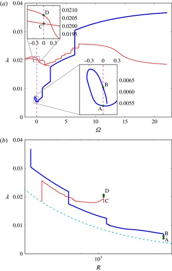
secondary flow, were able to be continued to channel flow solutions. The homotopy paths of these two flows are shown in figure 1, where the friction factor
 $$\begin{eqnarray}{\it\lambda}=\frac{2LJ}{{\it\rho}{u_{m}^{\ast }}^{2}}=\frac{16R}{\displaystyle \left(\int _{-1}^{1}\overline{u}\,\text{d}y\right)^{2}},\end{eqnarray}$$
in which
 $u_{m}^{\ast }$
denotes the average of the dimensional mean flow, is used as a nonlinear measure. The
 $\mathscr{G}_{1}$
seed flow was obtained as a tertiary flow bifurcating superharmonically from a streamwise-independent secondary flow examined by Wall & Nagata (Reference Wall and Nagata2006). Here ‘superharmonic’ means that the spanwise wavenumber of the tertiary flow is the same as that of the secondary flow it bifurcates from. In particular, this seed flow has parameters
 $(R,{\it\Omega})=(430,22.1325)$
. The
 $\mathscr{G}_{13}$
seed flow is instead a secondary flow, bifurcating directly from the basic flow, with the parameters of the present seed flow given by
 $(R,{\it\Omega})=(494,22.1325)$
. Further details of all flows, including those of the 13 flows that failed to be continued to the channel flow case, are given in Wall & Nagata (Reference Wall and Nagata2013).
For the
 $\mathscr{G}_{1}$
flow
 ${\it\Omega}$
can be reduced to 6.48 before
 $R$
must first be increased, and two further large increases and one small increase in
 $R$
are used to continue the bifurcation curve across the
 ${\it\Omega}=0$
axis (point A in figure 1) at
 $R=2253$
. Continuing to decrease
 ${\it\Omega}$
further, a turning point is passed at
 ${\it\Omega}=-0.35$
, with then a second branch of this channel flow solution obtained at point B in figure 1. We henceforth label the (non-rotating) channel flow solution marked by points A and B that originated from this
 $\mathscr{G}_{1}$
seed as TW1.
For the
 $\mathscr{G}_{13}$
flow
 ${\it\Omega}$
can be decreased from 22.1325 to 7.16 at the initial seed value of
 $R$
, before the homotopy proceeds through many cycles increasing
 $R$
then decreasing
 ${\it\Omega}$
until the bifurcation curve crosses the
 ${\it\Omega}=0$
axis with
 $R=1068$
(point C in figure 1). This solution can also be followed around a turning point in
 ${\it\Omega}$
at
 ${\it\Omega}=-1.91$
before a second solution branch for this flow is obtained as marked by point D in figure 1. We henceforth label the (non-rotating) channel flow solution marked by points C and D that originated from this
 $\mathscr{G}_{13}$
seed as TW2.
3.2. Flow symmetries
All the symmetries relevant to the present flows are listed in the following relations,
 $$\begin{eqnarray}\displaystyle & \displaystyle T:\left[u,v,w\right](x,y,z)=\left[u,v,-w\right](x+{\rm\pi}/{\it\alpha},y,-z), & \displaystyle\end{eqnarray}$$
 $$\begin{eqnarray}\displaystyle & \displaystyle S:[u,v,w](x,y,z)=[u,v,-w](x+{\rm\pi}/{\it\alpha},y,{\rm\pi}/{\it\beta}-z), & \displaystyle\end{eqnarray}$$
 $$\begin{eqnarray}\displaystyle & \displaystyle Z_{z}:\left[u,v,w\right](x,y,z)=\left[u,v,-w\right](x,y,-z), & \displaystyle\end{eqnarray}$$
 $$\begin{eqnarray}\displaystyle & \displaystyle R:[u,v,w](x,y,z)=[u,-v,-w](x,-y,-z), & \displaystyle\end{eqnarray}$$
 $$\begin{eqnarray}\displaystyle & \displaystyle Z_{y}[u,v,w](x,y,z)=[u,-v,w](x,-y,z), & \displaystyle\end{eqnarray}$$
 $$\begin{eqnarray}\displaystyle & \displaystyle Z_{zy}[u,v,w](x,y,z)=[u,-v,-w](x,-y,{\rm\pi}/{\it\beta}-z). & \displaystyle\end{eqnarray}$$
As can be understood from a physical argument based on the inviscid criterion of Pedley (Reference Pedley1969) for example, rotation of channel flow about a spanwise axis introduces an asymmetry about the channel centreplane (
 $y=0$
), whereby one half of the channel (the anticyclonic half) becomes destabilised by the rotation while the other half (the cyclonic half) is stabilised by the rotation. Accordingly, all of the three-dimensional exact coherent states for rotating channel flow presented by Wall & Nagata (Reference Wall and Nagata2013) are asymmetrical about the channel centreplane. Neither of the two channel flows TW1 and TW2 have regained symmetry about this plane in the non-rotating channel case, i.e. they are both asymmetric about the channel centreplane. However, both flows retain the symmetries they possess when
 ${\it\Omega}\neq 0$
. Specifically, the TW1 solution satisfies the shift-and-reflect symmetry (3.2), which is equivalent to (5.1) of Wall & Nagata (Reference Wall and Nagata2013). Note that this symmetry is also equivalent to the ‘
 $S$
’ symmetry (3.3) of Nagata & Deguchi (Reference Nagata and Deguchi2013) under the change of coordinates
 $\tilde{x}=x$
,
 ${\tilde{y}}=y$
,
 $\tilde{z}=z-{\rm\pi}/(2{\it\beta})$
(the placement of the origin in the spanwise direction is of course arbitrary).
The present TW2 solution satisfies the
 $S$
symmetry (3.3) described above (equivalent to equation (5.3) of Wall & Nagata (Reference Wall and Nagata2013)), together with the reflectional symmetry (3.4) (equivalent to equation (5.2) of Wall & Nagata (Reference Wall and Nagata2013)).
The present study also presents a third channel flow solution, TW3, which the TW1 flow bifurcates from. As well as the shift-and-reflect symmetry (3.2), this flow is also invariant under symmetry (3.5) which describes a rotation of
 ${\rm\pi}$
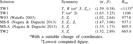
about a streamwise axis through the origin. The other symmetries (3.6) and (3.7) are defined in order to compare with the results of previous studies. The symmetries of the present flows are summarised in table 1.
Summary of the symmetries and optimum wavenumber pairs of the present channel-flow solutions, and other channel-flow solutions for which data is available.

a With a suitable change of coordinates.
b Lowest computed figure.
3.3. Bifurcation structure and optimal wavenumber pairs
The wavenumbers of the TW1 and TW2 channel flow solutions obtained by homotopy from rotating channel-flow solutions as described in § 3.1 above are optimized in order to identify the minimum value of
 $R$
at which these solutions first appear (all of the present solutions first appear in a saddle–node bifurcation with increasing
 $R$
). Such an optimisation thus yields a global minimisation problem for
 $R$
over two variables,
 ${\it\alpha}$
and
 ${\it\beta}$
. This problem was solved by fixing
 $R$
at slightly above an initial lowest value of
 $R$
, and first performing homotopies in
 ${\it\alpha}$
and
 ${\it\beta}$
to delineate the existence region of the solution in the
 $({\it\alpha},{\it\beta})$
plane at this
 $R$
. Such a process yields a grid of solutions in the
 $({\it\alpha},{\it\beta})$
plane. Next, starting from each such grid point, where each grid point thus denotes a wavenumber pair
 $({\it\alpha},{\it\beta})$
, we homotopy in the direction of decreasing
 $R$
to determine a new lowest value of
 $R$
from among all these wavenumber pairs. Fixing
 $R$
slightly above this value, we then repeat the process described above. Note in general the existence region in the
 $({\it\alpha},{\it\beta})$
plane depends on
 $R$
, and in particular the existence region at a given value of
 $R$
is not guaranteed to lie within the same solution’s existence region at a higher value of
 $R$
, which necessitates the iterative process described above. Finally, once an approximate value for the minimum value of
 $R$
and corresponding optimum wavenumbers
 $({\it\alpha},{\it\beta})$
have been obtained by this brute force approach, a more accurate figure is obtained using the constrained minimisation algorithm developed by Byrd et al. (Reference Byrd, Lu, Nocedal and Zhu1995).
The TW1 flow is found to first appear in a saddle–node bifurcation at
 $R=1106$
for
 $({\it\alpha},{\it\beta})=(1.63,3.25)$
. As shown in figure 3, for this wavenumber pair, the upper branch of the optimum TW1 flow passes through a number of turning points before moving in the direction of increasing
 $R$
as far as the flow has been tracked (to
 $R=3000$
). The lower branch of the bifurcation curve can be followed through 4 turning points before it then terminates at around
 $R=1403$
. An examination of the solution at this point reveals that the flow is assumes a structure that exhibits a half-turn rotational symmetry about a streamwise axis through a point on the channel centreplane. Anticipating that this termination point corresponds to a bifurcation point at which the present asymmetric flow TW1 bifurcates from a channel-flow solution that has additional symmetries, we used the present solution as an initial guess to obtain the third extended channel flow solution, TW3, that is presented in this study, which is also shown in figure 3 for the same wavenumbers. Note, in particular, that the symmetries this TW3 flow satisfies,
 $T$
and
 $R$
in § 3.2, are distinct to those satisfied by the flow presented by Waleffe (Reference Waleffe2003), whose flow satisfied mirror symmetry about the channel centreplane. An optimum wavenumber pair for the TW3 could not be precisely determined since a search found that this optimum appeared to be approaching a limit in which
 ${\it\beta}$
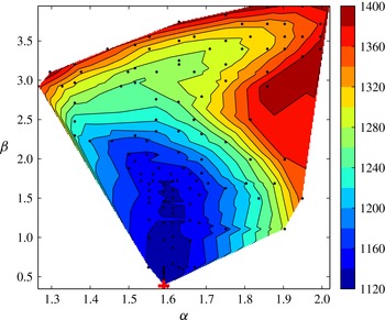
becomes small or zero, in which limit the number of Fourier modes in the spanwise direction required to maintain resolution becomes prohibitively expensive. Contours of the minimum Reynolds number in the (
 ${\it\alpha}$
,
 ${\it\beta}$
) plane for this flow are shown in figure 2. It can be seen that the optimum streamwise wavenumber appears to be approaching a limit that is approximately
 ${\it\alpha}=1.6$
, but this value also cannot be precisely determined without further calculations that are beyond the scope of the authors’ computational resources. The reason for this computational difficulty is that the solution in this limit is approaching a spanwise-localised solution, as is further discussed in § 3.5. However, we can report that the value of
 $R$
at which this solution first appears is at least as small as
 $R=1133$
(obtained for
 $({\it\alpha},{\it\beta})=(1.59,0.38)$
), and so this flow may also therefore be relevant to the early stages of transition in plane Poiseuille flow.
Contours of the minimum Reynolds number in the
 $({\it\alpha},{\it\beta})$
plane for the TW3 flow. The minimum appears to occur in the limit as
 ${\it\beta}$
becomes small, but cannot be precisely determined since computations become increasingly expensive in this limit. However, we have that
 $\min R\leqslant \min R({\it\alpha}=1.59,{\it\beta}=0.38)=1133$
(marked by the red cross).

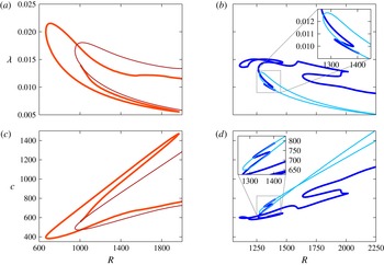
Friction factor (a,b) and wavespeed (c,d) against Reynolds number for channel flows (a,c): TW2 (thick orange line) and MS-S (thin red line) and (b,d): TW1 (thick dark blue line) and TW3 (thin light-blue line). The TW2 and MS-S curves are plotted for the optimum wavenumber pair of the TW2 flow,
 $({\it\alpha},{\it\beta})=(1.32,2.89)$
, while the TW1 and TW3 curves are plotted for the optimum wavenumber pair of the TW1 flow,
 $({\it\alpha},{\it\beta})=(1.63,3.25)$
. The TW2 solution provides, to our knowledge, the lowest Reynolds number at which channel flow solutions other than the basic flow are known to exist (the solution appears in a saddle–node bifurcation at
 $R=665$
). The TW2 flow is asymmetric with respect to the channel centreplane and bifurcates as shown from the mirror-symmetric MS-S flow. The TW1 flow is also asymmetric and bifurcates from the TW3 flow, which satisfies a half-turn symmetry about a streamwise axis through a point on the channel centreplane.

The TW2 flow is found to first appear in a saddle–node bifurcation at
 $R=665.4$
for
 $({\it\alpha},{\it\beta})=(1.32,2.89)$
. To our knowledge, this flow thus represents the lowest known channel flow solution in
 $R$
aside from the basic flow, substantially reducing the value 805.5 of the lowest Reynolds number at which such solutions have hitherto been identified (this latter figure corresponds to the recently presented MS-A flow of Nagata & Deguchi (Reference Nagata and Deguchi2013)). The bifurcation curve for the TW2 increases as far as
 $R=1968$
, whereupon it goes around a turning point and then decreases as far as
 $R=1008$
, where the solution appears to be approaching a termination point, i.e. a point at which solution bifurcates from another invariant solution. Using this present solution as an initial guess, we obtained a fourth travelling-wave solution that satisfies the mirror symmetry about the channel centreplane
 $Z_{y}$
in addition to the two symmetries,
 $S$
and
 $Z_{z}$
, satisfied by the TW2 flow. Noting the similarities of the flow structures (not shown) with those of the MS-S flow described by Nagata & Deguchi (Reference Nagata and Deguchi2013), we confirmed that these two flows are the same by calculating the optimal wavenumber pair
 $({\it\alpha},{\it\beta})=(1.47,3.06)$
, corresponding to a saddle–node bifurcation at
 $R=937.1$
, in agreement with the figures of Nagata & Deguchi (Reference Nagata and Deguchi2013). The bifurcation curve for this MS-S flow is also shown in figure 3, both upper and lower branches continue without encountering turning points in the direction of increasing
 $R$
as far as they have been tracked, to
 $R=4700$
and
 $R=3\times 10^{4}$
, respectively.
Figure 3 also plots the corresponding wavespeeds of the flows. It can be seen that, away from turning points, the wavespeed of all the flows increases with
 $R$
, while it may be noted that in all cases the upper (lower) branch of the friction factor curves correspond to the lower (upper) branch of the wavespeed curves; that is in both cases a higher friction factor corresponds to lower wavespeeds, as has been observed for invariant solutions in other shear flows, see for example Kerswell (Reference Kerswell2005) or Faisst & Eckhardt (Reference Faisst and Eckhardt2003).
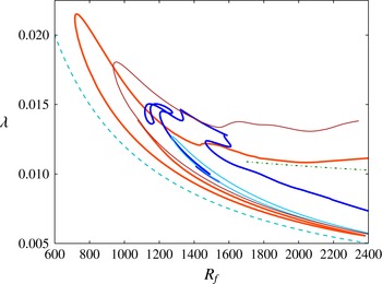
For reference, we also include in figure 4 a plot of the friction factor against a flux-based Reynolds number
 $R_{f}=\int _{-1}^{1}\overline{u}\,\text{d}y$
, along with the corresponding laminar relationship and also Patel & Head (Reference Patel and Head1969)’s empirical law for turbulent flow. All of the lower branches lie close to the laminar values, while the TW1 and TW2 upper branches appear to lie either side of the empirical turbulent value.
Friction factor plotted against a flux-based Reynolds number
 $R_{f}$
for the present travelling-wave solutions. Parameters are as in figure 3, and corresponding line colours/thicknesses have been used here. Also shown are the laminar friction factor (light blue, dashed line), and Patel & Head (Reference Patel and Head1969)’s empirical friction factor law for turbulent flow,
 ${\it\lambda}=0.0376R_{f}^{-1/6}$
(green, dot-dashed line).

3.4. Flow structures
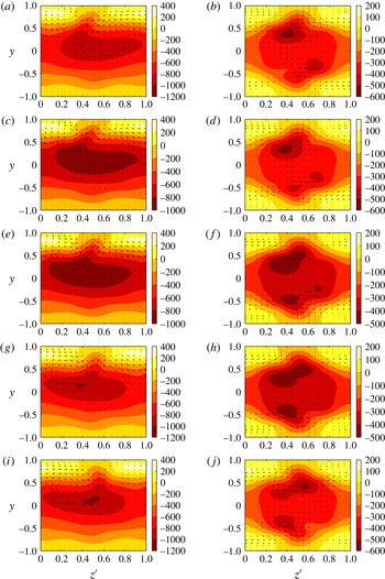
The disturbance velocities of the TW1 flow in a spanwise wall-normal projection are shown in figure 5. These plots, which exclude the basic flow, show that the disturbance velocity for the upper branch of this flow is characterised by one large, strong low-speed streak in the centre of the channel and one weaker high-speed streak adjacent to the wall, per spanwise wavelength. The two streaks are approximately half a spanwise wavelength apart. It may be seen that the flow in the lower-half of the channel (
 $y<0$
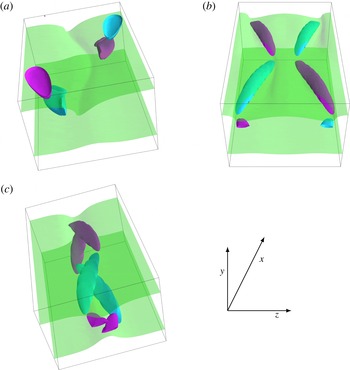
) is relatively undisturbed in comparison with the upper-half of the channel. In contrast, for the lower-branch of this flow there are large disturbances in both halves of the channel, which is in agreement with the fact that this flow is approaching the half-turn rotationally symmetric TW3 flow along this branch. A three-dimensional visualisation of the upper branch flow is shown in figure 8. The plot shows isosurfaces of the streamwise component of total velocity (i.e. including the basic flow), and of the streamwise component of vorticity. The total streamwise velocity of this flow is characterised by a sinusoidal low-speed streak in the upper-half of the channel, with vortex structures occurring staggered either side of this streak, with those beneath the velocity isosurface tilted down towards the centre of the channel with movement in the streamwise direction, while the patches of vorticity close to the upper channel wall are, in contrast, approximately horizontally aligned. These structures clearly share qualitative similarities with those of Waleffe’s (Reference Waleffe2003) solution, see for example his figure 15, and may perhaps be regarded as an asymmetric version of Waleffe’s (Reference Waleffe2003) flow.
Disturbance velocity of the TW1 flow in a spanwise wall-normal projection. One strong low-speed streak is flanked by staggered vortical structures. For the upper-branch, flow in the lower-half of the channel is relatively undisturbed from the laminar state, while the lower-branch flow is approaching the half-turn rotationally symmetric TW3 flow. Velocity vectors in this projection are shown plotted on contours of the streamwise component of the disturbance velocity at streamwise stations
 $x=(2{\rm\pi}/{\it\alpha})(i/10),\;i=$
(a,b) 0, (c,d) 1, (e,f) 2, (g,h) 3, (i,j) 4 for (a,c,e,g,i) the upper-branch flow with
 $(R,{\it\alpha},{\it\beta})=(1750,1.63,3.25)$
and (b,d,f,h,j) the lower-branch flow with
 $(R,{\it\alpha},{\it\beta})=(1300,1.63,3.25)$
. One wavelength is shown in
 $z^{\prime }=(1/2{\rm\pi})({\it\beta}z)$
, while plots for
 $i=5,\ldots ,9$
may be obtained from the above plots with reference to the symmetries discussed in § 3.2.

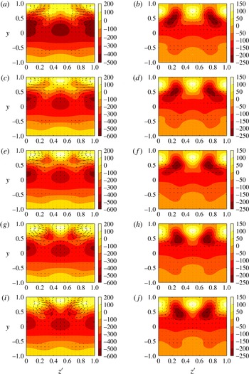
The plots of the disturbance velocities of the TW2 flow in figure 6, show that this flow is characterised by two low-speed and two high-speed streaks per spanwise wavelength, where the high-speed streaks are located close to the upper wall as for the TW1 flow. The upper-branch flow clearly exhibits a two-layer structure in the upper half of the channel (see figure 6
c for example), which it has inherited from the
 $\mathscr{G}_{13}$
seed flow from which it has been derived. The lower-branch flow does not so clearly exhibit such a two-layer structure, while the location of the low-speed streaks is also different from that of the upper-branch; the latter features low-speed streaks located at approximately the same spanwise location as the high-speed streaks whereas the former has low-speed streaks that are one quarter of one spanwise wavelength away from the location of the high-speed streaks, and are closer to the upper wall. Similar to the TW1 upper branch flow, the disturbance to the basic flow is much weaker in the lower half of the channel. The upper-branch TW2 flow is also visualised in figure 8, which shows the large spanwise movement of these flow structures as the wave moves through the channel.
Disturbance velocity of the TW2 flow in a spanwise wall-normal projection. This flow features two low-speed streaks per spanwise wavelength and a double-layered structure in the upper-half of the channel (more visible for the upper-branch solution), while the lower-half of the channel is relatively undisturbed from the laminar state. Velocity vectors in this projection are shown plotted on contours of the streamwise component of disturbance velocity at streamwise stations
 $x=(2{\rm\pi}/{\it\alpha})(i/10)$
,
 $i=$
(a,b) 0, (c,d) 1, (e,f) 2, (g,h) 3, (i,j) 4 for (a,c,e,g,i) the upper-branch flow and (b,d,f,h,j) the lower-branch flow both with
 $(R,{\it\alpha},{\it\beta})=(1200,1.32,2.89)$
. One wavelength is shown in
 $z^{\prime }=(1/2{\rm\pi})({\it\beta}z)$
, while plots for
 $i=5,\ldots ,9$
may be obtained from the above plots with reference to the symmetries discussed in § 3.2.

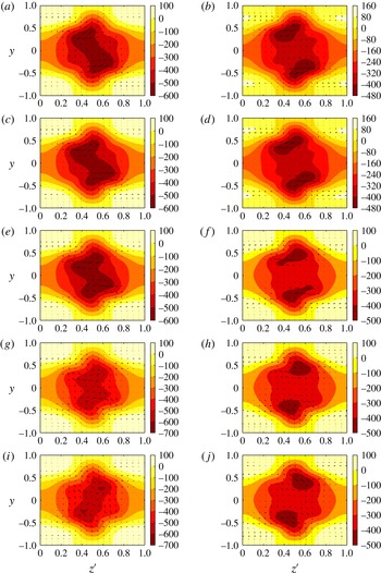
The disturbance velocities of the TW3 flow are shown in figure 7. This flow is characterised by a single strong low-speed velocity streak located on the centreline of the channel and a much weaker single high-speed streak in each half of the channel located near the channel walls. The corresponding three-dimensional visualisation of the upper-branch flow in figure 8 shows that the disturbance is largely concentrated in a central core region. The corresponding plot for the lower-branch flow is qualitatively similar.
Disturbance velocity of the TW3 flow in a spanwise wall-normal projection. This flow is symmetric under a rotation of
 ${\rm\pi}$
about a streamwise axis through a point on the channel centreplane, and features one strong low-speed streak in each half of the channel. Velocity vectors in this projection are shown plotted on contours of the streamwise component of disturbance velocity at streamwise stations
 $x=(2{\rm\pi}/{\it\alpha})(i/10),\;i=$
(a,b) 0, (c,d) 1, (e,f) 2, (g,h) 3, (i,j) 4 for (a,c,e,g,i) the upper-branch flow and (b,d,f,h,j) the lower-branch flow both with
 $(R,{\it\alpha},{\it\beta})=(1500,1.63,3.25)$
. One wavelength is shown in
 $z^{\prime }=(1/2{\rm\pi})({\it\beta}z)$
, while plots for
 $i=5,\ldots ,9$
may be obtained from the above plots with reference to the symmetries discussed in § 3.2.

Visualisation of the flow structures of (a) TW1, (b) TW2 and (c) TW3. The TW1 and TW3 flows feature one low-speed streak per spanwise wavelength while the TW2 flow features two such streaks. The TW1 and TW2 flows are asymmetric about the channel centreplane while the TW3 flow has half-turn rotational symmetry about a streamwise axis through a point on this plane. The blue (purple) isosurfaces show 0.7 of the minimum (maximum) of the streamwise component of vorticity, while the translucent sheets show isosurfaces of 0.5 of the maximum of the streamwise component of velocity. Flow parameters correspond to the upper-branch flows plotted in (a) figure 5, (b) figure 6 and (c) figure 7.

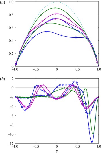
In figure 9 we plot the mean flow for the present channel flow solutions. It can be seen that all the flows are inflectional; the one exception in the present plots is the upper branch of the TW2 solution, but we have verified that this flow also becomes inflectional further along this branch. (The existence of inflection points is necessary (although not sufficient) for instability of an inviscid flow as described by Drazin & Reid (Reference Drazin and Reid1981) for example, and is often observed to correspond to reduced stability of viscous flows, see the discussion of Sengupta (Reference Sengupta2012) for example.) The TW1 upper branch solution and the TW2 solutions retain a quasi-parabolic mean flow profile in the lower half of the channel, in agreement with the plots of figures 5, 6 and 8, which show only small disturbances to the basic state in this region of the channel. By contrast, the TW3 solutions, and the TW1 lower-branch solution, which is becoming like the TW3 profile it bifurcates from as it approaches this bifurcation point, exhibit inflection points in both halves of the channel.
(a) Mean flow
 $u_{0}(y)+{\check{U}}(y)$
and (b)
 $u_{0}^{\prime \prime }(y)+{\check{U}}^{\prime \prime }(y)$
for the present channel flow solutions. All the flows TW1, TW2 and TW3 feature inflection points. Blue (▫) TW1 upper-branch, parameters as figure 5(a,c,e,g,i), blue (♢) TW1 lower-branch, parameters as figure 5(b,d,f,h,j); green (
 $+$
) TW2 upper-branch, parameters as figure 6(a,c,e,g,i), green (
 $\times$
) TW2 lower-branch, parameters as figure 6(b,d,f,h,j); magenta (▵) TW3 upper-branch, parameters as figure 7(a,c,e,g,i), magenta (▿) TW3 lower-branch, parameters as figure 7(b,d,f,h,j). The dashed line in (a) shows the laminar profile.

3.5. Spanwise-localised solutions
In an effort to address the spatio-temporal intermittency that is observed in transitionary shear flows, several recent studies have sought solutions that are spatially localised in the spanwise and/or the streamwise directions. We intend to pursue the localised counterparts of the present extended solutions as part of a future study using a purpose-built numerical code. However, the present TW3 flow, for which the disturbance to the basic flow is concentrated in a core region in the spanwise direction as shown in figures 7 and 8, has a structure which suggests the derivation of a spanwise-localised solution may be practicable with the present numerical method. Previous studies have employed either a window function (e.g. Gibson & Brand Reference Gibson and Brand2014), or have used continuation in a larger periodic box size (e.g. Zammert & Eckhardt Reference Zammert and Eckhardt2014b
) to extract a localised solution from an extended one. In the present approach, similar to the latter, we continue the spanwise wavenumber
 ${\it\beta}$
to smaller values to derive a spanwise localised solution, TW3-L.
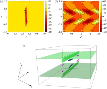
Visualisation of the flow structure of TW3-L, the spanwise-localised counterpart of the TW3 flow. Plotted are (a) disturbance velocity in a spanwise wall-normal projection, where the contours show the streamwise component of disturbance velocity, at
 $x=(2{\rm\pi}/10{\it\alpha})$
, (b) the fluctuating part of the streamwise component of disturbance vorticity in the streamwise wall-normal plane at
 $z={\rm\pi}/{\it\beta}$
, and (c) isosurfaces of the streamwise components of vorticity (the blue (purple) isosurfaces show 0.7 of the minimum (maximum) of this variable) and velocity (the translucent sheets show isosurfaces of 0.5 of the maximum of this variable). The low-speed velocity streaks show little variation in the streamwise direction, while the half-turn rotational symmetry about
 $(y,z)=(0,{\rm\pi}/{\it\beta})$
is preserved in the localisation. Flow parameters are
 $(R,{\it\alpha},{\it\beta})=(1158,1.59,0.197)$
, and in (a) and (b) one wavelength is shown in
 $z^{\prime }=(1/2{\rm\pi})({\it\beta}z)$
and two wavelengths in
 $x^{\prime }=(1/2{\rm\pi})({\it\alpha}x)$
respectively.

In figure 10(a) we show an instantaneous profile of the velocity of the flow in a spanwise wall-normal plane. Both the half-turn rotational symmetry (3.5) and the shift-reflect symmetry (3.2) are preserved in the spanwise localisation, and it can be seen that the flow is characterised by two low-speed streaks of the streamwise velocity component, one in the upper-half and one in the lower-half of the channel, which are located within a low-speed envelope. There are four much weaker high-speed streaks in the same velocity component located either side of both ends of the low-speed envelope. With movement along the channel in the streamwise direction, the low-speed streaks oscillate with small amplitude in the spanwise direction while the low-speed envelope shows little dependence on this direction. The latter can be seen from the plot of isosurfaces of streamwise vorticity and velocity shown in figure 10(c). The solution remains extended in the streamwise direction, and, as shown in figure 10(b), it can be seen that the vortex structures in the upper (lower) half of the channel are inclined downwards (upwards) towards the centre of the channel in the direction of increasing
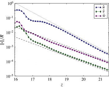
 $x$
. The decay of the tail of the solution with respect to movement in the spanwise direction is considered in figure 11, where, following Gibson & Brand (Reference Gibson and Brand2014) and Zammert & Eckhardt (Reference Zammert and Eckhardt2014b
), we measure the
 $\infty$
-norm of the disturbance velocity components
 $\hat{\boldsymbol{u}}=[\hat{u} ,\hat{v},{\hat{w}}]$
, where
 $\mathscr{L}_{\infty }(\hat{u} )=\max _{x,y}\!\Vert \hat{u} (x,y,z)\Vert$
, with corresponding expressions for the other components. It can be seen that all the velocity components decay approximately exponentially. Gibson & Brand (Reference Gibson and Brand2014) considered a linear normal mode-based model for the decay of the tails of spanwise localised solutions, which predicts that the components of disturbance velocity will all decay at the same rate or multiples of that rate. Applying this analysis to plane Couette flow, they found that the streamwise and spanwise components of the velocity disturbance decayed as
 $\text{e}^{-{\it\alpha}z}$
, while the wall-normal component decayed faster as
 $\text{e}^{-2{\it\alpha}z}$
. In contrast, for the present channel flow solution the spanwise and wall-normal components decay at the same rate, which is approximately
 $\text{e}^{-z}$
, while the streamwise component decays faster at approximately
 $\text{e}^{-1.44z}$
. However, in the present case the streamwise component of the disturbance velocity is of an order of magnitude larger than the other two components, and so its nonlinear interactions with these components cannot be neglected. It is possible, however, that the results we are able to compute for the present case represent an inner tail, and that with further decay an outer tail can be attained in which the linear assumption is valid.
Decay of the tail of the spanwise-localised solution TW3-L shown in figure 10. The
 $\mathscr{L}_{\infty }$
-norm of the disturbance velocity components scaled by
 $R$
show an exponential decay in the spanwise direction with the spanwise and wall-normal components decaying approximately as
 $\text{e}^{-z}$
(shown by the dashed lines (- - - -)), while the streamwise component decays as
 $\text{e}^{-1.44z}$
(shown by the dotted (
 $\cdots \cdots$
) line).

4. Stability and significance of solutions
In this section we analyse the stability and assess the relevance of the present solutions. We first selected a wavenumber pair
 $({\it\alpha},{\it\beta})=(1.5,3.1)$
at which all of the present flows exist, and continued by homotopy the solutions to the same Reynolds number
 $R=2300$
. We then considered the stability of these flows to fundamental disturbances, with the calculations performed using the ‘channelflow’ code designed and maintained by Gibson (Reference Gibson2013). This code also provides an independent numerical check of the homotopy calculations; for example, fixing the wavenumber pair at the optimum values
 $({\it\alpha},{\it\beta})=(1.32,2.89)$
we determine the saddle–node bifurcation for the TW2 flow to occur at
 $R=665.4$
on a grid of dimensions
 $40\times 57\times 36$
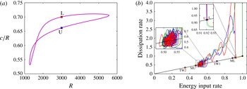
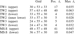
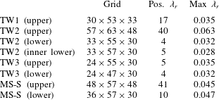
, in agreement with the results of § 3.3. The results of the stability analysis are presented in table 2. It can be seen that all the flows are unstable in relatively few directions, with the spectrum for the TW2 upper branch flow featuring the largest growth rate. With the exception of the TW3 upper branch flow, and in agreement with expectations, the spectra for the upper branch flows feature a larger number of unstable directions than those of the lower branch flows. The reason for the TW3 upper flow featuring such a low number of unstable directions is that, as shown in figure 12(a), this solution exists on an isolated (i.e. closed) bifurcation branch that extends across the range of transitionary Reynolds numbers, with the upper and lower branches lying relatively close to each other. We speculated that both upper and lower branches, i.e. the whole of the bifurcation curve, lie on the boundary basin (the separatrix separating initial conditions that lead to long-lived turbulence or turbulent events from those that decay to the laminar flow), and performed simulations, again using the ‘channelflow’ code, to further investigate these solutions. The results of simulations performed at
 $R=3000$
are shown in figure 12(b), where we show input energy rate versus dissipation rate. Long-lived turbulence is possible at this value of
 $R$
, as can be seen, for example, with respect to the simulation that starts from the perturbed laminar flow, which remains turbulent throughout the
 $5\times 10^{4}$
time units of the simulation. The simulations confirm that both upper and lower branches of the TW3 flow lie on the boundary basin; simulations with initial conditions given by these solutions with the addition of a perturbation either proceed to long-lived turbulence or slowly decay back to the laminar flow on a viscous time scale depending on the perturbation. The TW1 and TW2 upper branch solutions are also included in figure 12(b). Neither is visited by the turbulent state in the present simulations, with the turbulent flow lying between these two solutions in agreement with the results for the friction factor presented in figure 4. The MS-S upper and lower branches also lie either side of the turbulent state; in this projection, the upper branch solution lies closer than any of the other flows to the turbulent state, but is not visited in the present simulations. (Note that the TW2 lower branch passes through a turning point at
 $R=2670$
and then terminates in a bifurcation point from another invariant solution as described for another wavenumber pair in § 3.1, and so does not exist at
 $R=3000$
.)
(a) The isolated bifurcation branch of the TW3 solution, scaled wavespeed against
 $R$
with the upper (blue square, ‘U’) and lower (red square, ‘L’) branch solutions at
 $R=3000$
marked. (b) Simulations at
 $R=3000$
starting from the laminar flow (black filled circle (●)) and the upper (blue square, ‘U’) and lower (red square, ‘L’) branches of the TW3 flow showing input energy rate against rate of energy dissipation (both quantities are scaled so that the laminar flow lies at (1, 1)). Both branches of the TW3 isolated bifurcation branch lie on the boundary basin between flows that decay to laminar flow and those that evolve to long-lived turbulence or turbulent events. Also marked are the TW1 and TW2 upper branch solutions, which lie either side of the turbulent state, and the upper (MU) and lower (ML) branches of the MS-S flow. All travelling-wave solutions are obtained for
 $({\it\alpha},{\it\beta})=(1.5,3.1)$
, while simulations are performed on the corresponding box size,
 $L_{x}\times L_{z}=2{\rm\pi}/{\it\alpha}\times 2{\rm\pi}/{\it\beta}$
.

Stability of the travelling-wave solutions, TW1, TW2, TW3 and MS-S to fundamental disturbances. Stability calculations are performed using the channelflow software, and the triplet in the second column denotes the channelflow number of grid points in the streamwise, wall-normal and spanwise directions, respectively, while the third column displays the number of unstable directions of each flow and the fourth column the maximum real part of eigenvalues with positive real part, expressed in terms of the same time units as used in the study of Gibson & Brand (Reference Gibson and Brand2014). All calculations are performed for
 $(R,{\it\alpha},{\it\beta})=(2300,1.5,3.1)$
.
5. Conclusions and discussion
In the present study, exact coherent state channel-flow solutions have been obtained by continuing solutions obtained for channel flow subject to a system rotation about a spanwise axis to non-rotating channel flow by homotopy. In particular, it was possible to continue two of the 15 distinct rotating channel-flow solutions reported by Wall & Nagata (Reference Wall and Nagata2013) to the non-rotating case to yield spatially extended channel-flow solutions, labelled TW1 and TW2 in the present study. Both of these flows are asymmetric about the channel centreplane. However, a third extended flow, TW3, that satisfies a half-turn rotational symmetry about a streamwise axis through a point on the channel centreplane, is additionally found to be the flow from which TW1 bifurcates in a symmetry-breaking bifurcation, while the TW2 flow is found to bifurcate from the mirror symmetric MS-S flow previously investigated by Nagata & Deguchi (Reference Nagata and Deguchi2013).
The TW1 flow features one strong low-speed streak per spanwise wavelength in the streamwise component of velocity, while the TW2 flow features two such low-speed streaks. In both cases the streaks are sinusoidal and are flanked by staggered vortex structures. For the upper branch of the TW1 flow and both branches of the TW2 flow the disturbance to the flow in one half of the channel (the lower-half for the present plots) relative to that in the other half is much smaller. The structure of the lower branch of the TW1 flow approaches that of the TW3 flow, which has disturbances of equal magnitude in each half of the channel. The TW1 flow can perhaps be regarded as an asymmetric (with respect to the channel centreplane) version of Waleffe (Reference Waleffe2003)’s channel flow solution, since it shares all the main features of the latter flow other than symmetry about the channel centreplane.
The TW2 flow more closely resembles the MS-A flow recently presented by Nagata & Deguchi (Reference Nagata and Deguchi2013), but appears to be distinct to this latter flow since the minimum Reynolds numbers at which these two flows first appear, and the corresponding optimum wavenumbers, are markedly different. In particular, the present TW2 flow reduces the lowest known Reynolds number at which channel flow solutions other than the basic state are known to exist to 665, from the previous known minimum of 805.5 reported by Nagata & Deguchi (Reference Nagata and Deguchi2013) for their MS-A flow.
The structure of the present TW3 flow, in which the disturbance to the basic flow is concentrated in a central core region in a spanwise wall-normal projection, suggested the practicability of the derivation of a spanwise-localised solution, and such a solution, labelled TW3-L, has also been presented. The solution was obtained by continuation in decreasing spanwise wavenumber (equivalent to increasing spanwise box size) and yielded a flow structure in which two low-speed streaks in the streamwise velocity component are located within a low-speed envelope that shows almost no dependence on the streamwise direction. The tail of the solution is found to decay approximately exponentially, with the wall-normal and spanwise components of velocity decaying at the same rate while the streamwise component decays at a slightly faster rate. The localised flow retains both the half-turn rotational symmetry and the shift-reflect symmetry of the parent TW3 flow. The extended flow is found to exist on an isolated bifurcation branch that extends across the range of transitionary Reynolds numbers, whose upper and lower branches lie on the boundary basin separating initial conditions that lead to long-lived turbulent events and those that directly decay back to the laminar flow.
Gibson & Brand (Reference Gibson and Brand2014) have also recently presented exact solutions for channel flow. These authors’ focus was in deriving spanwise localised solutions as a step towards addressing the spatial intermittency of turbulence in channel flow, but in the process they also obtained three spatially periodic solutions. Of these three solutions, one (their TW1) is mirror symmetric about the channel centreplane, while another (their TW3) is asymmetric about this plane, and features six high-speed streaks per spanwise wavelength in a pattern that is highly localised adjacent to one of the channel walls. Neither of these two solutions would thus appear to correspond to any of the three flows of the present study. Gibson & Brand (Reference Gibson and Brand2014)’s TW2 flow, however, satisfies the same symmetries as the present TW2 flow (and Nagata & Deguchi (Reference Nagata and Deguchi2013)’s MS-A flow), as well as possessing similar structures; with reference to Gibson & Brand (Reference Gibson and Brand2014)’s figures 7(b) and 8(c,d), we can observe an asymmetric flow featuring two streak/vortex systems per spanwise wavelength. Gibson & Brand (Reference Gibson and Brand2014) present limited quantitative data concerning their spatially periodic flows, but we have attempted a comparison for the case they consider when
 $(R,{\it\alpha},{\it\beta})=(2300,1,2)$
. Since Gibson & Brand (Reference Gibson and Brand2014)’s flow features a strong two-layer structure and low-speed streaks that are spanwise aligned with the high-speed streaks, we have accordingly used our TW2 upper-branch for comparison (see § 3.4). However, Gibson & Brand (Reference Gibson and Brand2014)’s flow parameters appear to be close to the margin of the domain of existence of our TW2 flow; having fixed
 $R=2300$
and
 ${\it\beta}=2$
we were only able to increase
 ${\it\alpha}$
as far as 0.996, in which limit the disturbance to the lower half of the channel increases to be larger than that shown in Gibson & Brand (Reference Gibson and Brand2014)’s figures (and that shown in figure 6). We find a corresponding wavespeed in Gibson & Brand (Reference Gibson and Brand2014)’s units of
 $c_{x}=0.336$
, in comparison with Gibson & Brand (Reference Gibson and Brand2014)’s TW2 flow value of
 $c_{x}=0.564$
. Although only a limited comparison, these results would thus suggest that these two flows are distinct. Other asymmetric channel-flow solutions have been reported by Itano & Toh (Reference Itano and Toh2001), but the travelling waves described in their study feature a non-zero spanwise wave velocity component and so are distinct from the streamwise travelling waves of the present flows.
Regarding spanwise localised channel flow solutions, Gibson & Brand (Reference Gibson and Brand2014) present four such solutions derived from two of their spatially periodic flows. Their TW1-1 and TW1-2 flows retain the mirror symmetry about the channel centreplane the parent TW1 flow possesses, and thus are distinct to the present TW3-L flow, which instead satisfies a rotational half-turn symmetry about this plane. The other two flows are derived from Gibson & Brand (Reference Gibson and Brand2014)’s TW2 spatially extended flow described above; as part of future work it will be interesting to compare spanwise localised solutions derived from the present TW2 flow with these flows. Zammert & Eckhardt (Reference Zammert and Eckhardt2014a ) also discuss spanwise localised solutions, but these are asymmetric with respect to the channel centreplane unlike the present TW3-L flow. Furthermore, the extended flow from which Zammert & Eckhardt (Reference Zammert and Eckhardt2014a )’s flow is derived features one low- and one high-speed streak of equal strength, which does not correspond to either of the asymmetric spatially periodic flows considered here (Zammert & Eckhardt (Reference Zammert and Eckhardt2014a )’s flow is, besides, a chaotic edge state rather than a travelling-wave solution).
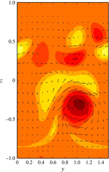
Velocity vectors projected in the wall-normal spanwise plane overlaying contours of streamwise vorticity for the upper branch TW1 solution at
 $(R,{\it\alpha},{\it\beta})=(3211,2,4.1)$
in comparison with figure 23 of Jimenez & Moin (Reference Jimenez and Moin1991). While the flow structures share similar features the Jimenez & Moin (Reference Jimenez and Moin1991) flow is more localised about the lower wall and exists for values of
 ${\it\beta}$
up to 5.71.

Channel flows that are asymmetric about the channel centreplane have been observed previously in the minimal flow unit study of Jimenez & Moin (Reference Jimenez and Moin1991). In their procedure, a minimal computational box size in which turbulence can occur is found by fixing a short streamwise box length (which corresponds to
 ${\it\alpha}=2$
), and then reducing the spanwise box width until the minimum size at which turbulence can still exist is obtained. An asymmetric flow is found to characterise the simulations, featuring a single low-speed streak per spanwise wavelength. Of the present flows, only TW1 features such flow structures, and we attempted to produce a corresponding channel flow invariant solution by a similar approach; first fixing
 ${\it\alpha}=2$
then increasing
 ${\it\beta}$
towards the value 5.71 derived in Jimenez & Moin (Reference Jimenez and Moin1991). Controlling the flux to correspond to Jimenez & Moin (Reference Jimenez and Moin1991)’s Reynolds number, we were, however, only able to increase
 ${\it\beta}$
to 4.1. In figure 13 we plot transverse velocity vectors overlaying contours of the streamwise vorticity, which may be compared with figure 23 of Jimenez & Moin (Reference Jimenez and Moin1991). It can be seen that while some features of the flow structures are similar, the Jimenez & Moin (Reference Jimenez and Moin1991) flow is more localised in the vicinity of the nearest wall, and further taking into account the discrepancy with the wavenumber existence domain described above, our tentative conclusion is thus that the present flow does not correspond to that observed in the Jimenez & Moin (Reference Jimenez and Moin1991) simulations.
Acknowledgement
D.P.W. would like to acknowledge the technical assistance of A. Togo, T. Noguchi and D. S. Wall.